The complex heavy-quark potential with the Gribov-Zwanziger action

Abstract

Gribov-Zwanziger prescription in Yang-Mills theory improves the infrared dynamics. In this work, we study the static potential of a heavy quark-antiquark pair with the HTL resummed perturbation method within the Gribov-Zwanziger approach at finite temperature. The real and imaginary parts of the heavy quark complex potential are obtained from the one-loop effective static gluon propagator. The one-loop effective gluon propagator is obtained by calculating the one-loop gluon self-energies containing the quark, gluon, and ghost loop. The gluon and ghost loops are modified in the presence of the Gribov parameter. We also calculate the decay width from the imaginary part of the potential. We also discuss the medium effect of heavy quark potential with the localized action via auxiliary fields.

I Introduction

Quarkonium suppression is one of the signatures of the creation of a novel state of quarks and gluons, i.e., quark-gluon plasma (QGP) Muller (1985) in relativistic heavy-ion collision experiments at the Large Hadron Collider (LHC) and Relativistic Heavy Ion Collider (RHIC). In 1986, Matsui and Satz Matsui and Satz (1986) suggested that the $J/\psi$ suppression due to Debye screening by color interaction in the medium can play an important role in QGP formation signature. The heavy quarkonium spectral functions are studied, theoretically, via approaches like Lattice QCD Satz (2007); Datta et al. (2004); Ding et al. (2012); Aarts et al. (2013a, b) and using effective field theories Brambilla et al. (2005); Bodwin et al. (1995); Brambilla et al. (2008). In an EFT, the study of quarkonium potential is not trivial, as the separation of scales is not always obvious. On the other hand, the lattice QCD simulation approach is used where spectral functions are computed from Euclidean meson correlation Alberico et al. (2008). As the temporal length at high temperatures decreases, the calculation of spectral functions is not straightforward, and the results highly depend on the discretization effect and have large statistical errors. So, the study of quarkonia at finite temperatures using the potential models Mocsy (2009); Wong (2005) are well accepted and has been investigated widely as a complement to lattice studies.

At high temperatures, the perturbative computations indicate that the potential of the quarkonia state is complex Laine et al. (2007). The real part is related to the screening effect due to the confinement of color charges Matsui and Satz (1986), and the imaginary part connects the thermal width to the resonance Beraudo et al. (2008). So, it was initially thought that the resonances dissociate when the screening is strong enough; in other words, the real part of the potential is too feeble to bind the $Q\bar{Q}$ pair together. In recent times, the melting of quarkonia is thought to be also because of the broadening of the resonance width occurring either from the gluon-mediated inelastic parton scattering mechanism aka Landau damping Laine et al. (2007) or from the hard gluon-dissociation method in which a color octet state is produced from a color singlet state Brambilla et al. (2013). The latter process is more important when the in-medium temperature is lesser than the binding energy of the resonance state. As a result, the quarkonium, even at lower temperatures, can be dissociated where the probability of color screening is insignificant. Gauge-gravity duality Hayata et al. (2013); Albacete et al. (2008) study also shows that the potential develops an imaginary component beyond a critical separation of the quark-antiquark pair. Lattice studies Rothkopf et al. (2012); Bala and Datta (2020) also talk about the existence of a finite imaginary part of the potential. Spectral extraction strategy Larsen et al. (2020); Bala et al. (2022) and the machine learning method Shi et al. (2022) have been recently used to calculate the heavy-quark (HQ) potential, both indicating a larger imaginary part of $Q\bar{Q}$ potential. All the studies of heavy quarkonium using potential models have been done within the perturbative resummation framework. In recent times, open quantum systems method Brambilla et al. (2021); Akamatsu (2022); Blaizot et al. (2016); Brambilla et al. (2018); Sharma and Tiwari (2020) is drawing more attention to the study of the quarkonium suppression in QGP matter. This method has also been applied to the framework of potential non-relativistic QCD, i.e., pNRQCD Brambilla et al. (2008); Escobedo and Soto (2008); Brambilla et al. (2013).

In the study of hot QCD matter, there are three scales of the system: hard scale, i.e., temperature $(T)$, (chromo)electric $gT$, and (chromo)magnetic scale $(g^{2}T)$, where $g$ is the QCD coupling. Hard thermal loop (HTL) resummed perturbation theory deals with the hard scale $T$ and the soft scale $gT$ but breaks down at magnetic scale $(g^{2}T)$, known as Linde problem Linde (1980); Gross et al. (1981). The physics in the magnetic scale is related to the nonperturbative nature. LQCD is appropriate to probe the nonperturbative behavior of QCD. Due to the difficulties in the computation of dynamical quantities with LQCD, it is useful to have an alternate technique to incorporate nonperturbative effects, which can be derived in a more analytical way, as in resummed perturbation theory. A formalism has been developed to incorporate the nonperturbative magnetic screening scale by employing the Gribov-Zwanziger (GZ) action Gribov (1978); Zwanziger (1989a) and it regulates the magnetic IR behavior of QCD. Since the gluon propagator with the GZ action is IR improved, this imitates confinement, causing the calculations to be more consistent with the results of functional methods and LQCD. Heavy quark diffusion coefficients Madni et al. (2023), quark number susceptibility and dilepton rate Bandyopadhyay et al. (2016), quark dispersion relations Su and Tywoniuk (2015), correlation length of mesons Sumit et al. (2023) have been studied using GZ action. Recent progress can be found in Refs. Sobreiro and Sorella (2005); Vandersickel and Zwanziger (2012); Dudal et al. (2008); Capri et al. (2016); Gotsman et al. (2021); Justo et al. (2022); Canfora et al. (2014).

In this article, we study the heavy quarkonium potential at finite temperatures within a non-perturbative resummation considering Gribov-Zwanziger action, which reflects the confining properties. In this direction, the heavy quark potential has been studied at zero temperature in recent times Gracey (2010). In Ref. Golterman et al. (2012), the HQ potential has been obtained considering the gluon propagator in the Coulomb gauge. We extend the zero temperature calculation to finite temperatures. This is performed from the Fourier transform of the effective gluon propagator in the static limit. The GZ prescription within the Landau gauge is reviewed briefly in Sec. II. The general structure of the gauge-boson propagator within the Gribov prescription has been constructed in Sec. III. The effective gluon propagator is calculated from the one-loop gluon self-energy in Sec. IV. In the presence of GZ action, we consider the effect of the Gribov parameter on the gluon and the ghost loop. We compute the real part of potential due to color screening and the imaginary part arising from the Landau damping in Sec. V. We have also evaluated thermal width for $J/\psi$ and $\Upsilon$. In Sec. VI, we discuss the medium effect on a local version of the Gribov action where the new set of auxiliary fields is introduced. In Ref. Wu et al. (2022), HQ potential is studied without considering Gribov modified ghost loop and auxiliary fields. In the present study, we have incorporated all those effects. Finally, in Sec. VII, we summarize our work..

II SETUP

We start with a brief overview of the semi-classical Gribov approach to QCD. The path-integral form of the Faddeev-Popov quantization procedure is

$$\mathcal{Z} = \int\mathcal{D}A\,\mathcal{D}\bar{c}\,\mathcal{D}c\,\,\delta(\partial\cdot A)\,\text{det}[-\partial\cdot A]$$ (1)

$$\times \exp\bigg{[}-S_{\text{YM}}-\int d^{4}x\,\bar{c}^{a}(x)\partial_{\mu}D_{\mu}^{ab}c^{b}(x)\bigg{]},$$

where $S_{\text{YM}}$ is the Yang-Mills action, $D_{\mu}^{ab}$ is covariant derivative in the adjoint representation of $SU(N)$. Additionally, $c$ and $\bar{c}$ are the ghost and anti-ghost fields. The above equation is ill-defined because of the presence of the Gribov copies Gribov (1978). To eliminate the copies, the integral is restricted to the Gribov region

$$\Omega=\{A:\partial\cdot A=0,-\partial\cdot D\geq 0\}$$ (2)

and this constrain can be realized by inserting the step function $V(\Omega)$ defined as

$$V(\Omega) = \theta[1-\sigma(P=0)]=\int_{-i\infty+\epsilon}^{+i\infty+\epsilon}\frac{e^{s(1-\sigma[0])}}{2\pi is}ds,$$ (3)

representing the no-pole condition (not going across the Gribov horizon) Fukushima and Su (2013); Vandersickel and Zwanziger (2012). By implementing the restriction, the generating functional reads

$$\mathcal{Z} = \int\mathcal{D}A\,\mathcal{D}\bar{c}\,\mathcal{D}c\,\text{det}[-\partial\cdot A]\,\delta(\partial\cdot A)\,V(\Omega)$$ (4)

$$\times\exp\bigg{[}-S_{\text{YM}}-\int d^{4}x\,\bar{c}^{a}(x)\partial_{\mu}D_{\mu}^{ab}c^{b}(x)\bigg{]}.$$

Defining the mass parameter $\gamma_{G}$ after minimizing the exponent of the integral (4) at some value of $s$, the following gap equation at one-loop order for Gribov mass parameter can be obtained as Vandersickel and Zwanziger (2012),

$$g^{2}\frac{(d-1)N_{c}}{d}\sum\!\!\!\!\!\!\!\!\!\int\limits_{P}\frac{1}{P^{4}+\gamma_{G}^{4}}=1.$$ (5)

$N_{c}$ is the number of colors and $d$ is the space-time dimension. The temporal component of the Euclidean four-momentum possesses discrete bosonic Matsubara frequencies. At asymptotically high temperatures, the form of the Gribov parameter simplifies as

$$\gamma_{G}=\frac{d-1}{d}\frac{N_{c}}{4\sqrt{2}\pi}g^{2}T.$$ (6)

The one-loop running coupling is

$$g^{2}(T)=4\pi\alpha_{s}=\frac{48\pi^{2}}{11N_{c}-2N_{f}}\frac{1}{\ln(\Lambda^{2}/\Lambda_{\overline{\text{MS}}}^{2})},$$ (7)

where the scale $\Lambda_{\overline{\text{MS}}}$ is fixed by requiring $\alpha_{s}(\Lambda=1.5\text{GeV})=0.326$ Bazavov et al. (2012) for $N_{f}=3$. The form of Gribov’s gluon propagator in Landau gauge is given by Gribov (1978); Zwanziger (1989a)

$$\Delta_{\mu\nu}^{0}(P)=\left(\delta_{\mu\nu}-\frac{P_{\mu}P_{\nu}}{P^{2}}\right)\frac{P^{2}}{P^{4}+\gamma_{G}^{4}},$$ (8)

where $\gamma_{G}$ is the Gribov parameter and $\delta_{\mu\nu}=(1,1,1,1)$. The appearance of the parameter $\gamma_{G}$ in the denominator shifts the pole of the gluon to the unphysical poles i.e. $P^{2}=\pm i\gamma_{G}^{2}$. This unphysical excitation using the Gribov parameter indicates the effective confinement of gluons. More detailed discussions about Gribov prescription can be found in review papers Vandersickel and Zwanziger (2012); Sobreiro and Sorella (2005); Dudal et al. (2008); Capri et al. (2016).

The ghost propagator in the Landau gauge with no-pole condition reads

$$D_{c}(P)=\frac{\delta^{ab}}{P^{2}}\frac{1}{1-\sigma(P)},$$ (9)

where, $(1-\sigma(P))^{-1}=Z_{G}$ is the ghost dressing function with

$$\sigma(P) = g^{2}N_{c}\frac{P_{\mu}P_{\nu}}{P^{2}}\sum\!\!\!\!\!\!\!\!\!\int\limits_{K}\frac{1}{K^{4}+\gamma_{G}^{4}}\frac{K^{2}}{(K-P)^{2}}$$ (10)

$$\times \bigg{(}\delta^{\mu\nu}-\frac{K^{\mu}K^{\nu}}{K^{2}}\bigg{)}.$$

Equation (9) in the infrared limit reduces to Vandersickel and Zwanziger (2012)

$$D_{c}(K^{2})=\frac{128\pi^{2}\gamma_{G}^{2}}{g^{2}N_{c}}\frac{1}{K^{4}},$$ (11)

indicating that ghost propagator is enhanced for $K\rightarrow 0$.

III General structure of gluon propagator with Gribov parameter

In this section, we construct the covariant form of the effective gluon propagator. In the vacuum, the gluon self-energy can be written as

$$\Pi^{\mu\nu}=\Pi(P^{2})\Big{(}\delta^{\mu\nu}-\frac{P^{\mu}P^{\nu}}{P^{2}}\Big{)}=\Pi(P^{2})V^{\mu\nu},$$ (12)

where $P^{\mu}=(p_{0},\bf{p})$ is the gluon four momentum and $\Pi(P^{2})$ is the Lorentz scalar depending upon $P^{2}$. In the presence of a thermal medium, the heat bath velocity $u^{\mu}$ is introduced. We can choose the rest frame of the heat bath i.e., $u^{\mu}=(1,0,0,0)$. In a thermal medium, the general structure of gluon self-energy can be written in terms of two independent symmetric tensors, as

$$\Pi^{\mu\nu}=\Pi_{T}A^{\mu\nu}+\Pi_{L}B^{\mu\nu},$$ (13)

where the forms of tensors are $B^{\mu\nu}=\frac{\bar{u}^{\mu}\bar{u}^{\nu}}{\bar{u}^{2}}$ with $\bar{u}^{\mu}=V^{\mu\nu}u_{\nu}$ and $A^{\mu\nu}=V^{\mu\nu}-B^{\mu\nu}$. The form factors $\Pi_{L}$ and $\Pi_{T}$ are functions of two Lorentz scalars $p_{0}$ and $p=|\bf{p}|$.

The effective gluon propagator can be written using Dyson-Schwinger equation as

$$\Delta_{\mu\nu}^{-1} = \left(\Delta_{\mu\nu}^{0}\right)^{-1}-\Pi_{\mu\nu}.$$ (14)

Here we would use the form of the gluon propagator as Su and Tywoniuk (2015)

$$\Delta_{\mu\nu}^{0}(P)=\left(\delta_{\mu\nu}-(1-\xi)\frac{P_{\mu}P_{\nu}}{P^{2}}\right)\frac{P^{2}}{P^{4}+\gamma_{G}^{4}},$$ (15)

where $\xi$ is the gauge parameter. This form is useful to invert the propagator. In the final expression of the effective gluon propagator, we put $\xi=0$. The form of the inverse gluon propagator from Eq. (15) reads as

$$\left(\Delta_{\mu\nu}^{0}\right)^{-1}=\left(\delta_{\mu\nu}-\frac{\xi-1}{\xi}\frac{P_{\mu}P_{\nu}}{P^{2}}\right)\frac{P^{4}+\gamma_{G}^{4}}{P^{2}}.$$ (16)

Putting the form of $\left(\Delta_{\mu\nu}^{0}\right)^{-1}$ in eq. (14), one gets the expression of inverse effective gluon propagator

$$\Delta_{\mu\nu}^{-1} = \frac{P^{4}+\gamma_{G}^{4}}{P^{2}\xi}\delta_{\mu\nu}+\left(\frac{\xi-1}{\xi}\frac{P^{4}+\gamma_{G}^{4}}{P^{2}}-\Pi_{T}\right)A_{\mu\nu}$$ (17)

$$+ \left(\frac{\xi-1}{\xi}\frac{P^{4}+\gamma_{G}^{4}}{P^{2}}-\Pi_{L}\right)B_{\mu\nu}.$$

To find the effective gluon propagator, one can write the general structure of gluon propagator in the tensor basis as,

$$\Delta_{\mu\nu}=\alpha P_{\mu}P_{\nu}+\beta A_{\mu\nu}+\gamma B_{\mu\nu},$$ (18)

where we need to find the coefficients $\alpha,\beta,\gamma$. Then we use the relation $\delta^{\nu}_{\alpha}=\Delta^{\mu\nu}\left(\Delta_{\mu\alpha}\right)^{-1}$ to obtaine the coefficients $\alpha,\beta,\gamma$ as

$$\beta = \frac{P^{2}}{P^{4}+\gamma_{G}^{4}-P^{2}\Pi_{T}},$$

$$\gamma = \frac{P^{2}}{P^{4}+\gamma_{G}^{4}-P^{2}\Pi_{L}},$$

$$\alpha = \frac{\xi}{P^{4}+\gamma_{G}^{4}}.$$ (19)

So, in-medium gluon propagator with Gribov term can be written as

$$\Delta_{\mu\nu} = \frac{\xi P_{\mu}P_{\nu}}{P^{4}+\gamma_{G}^{4}}+\frac{P^{2}A_{\mu\nu}}{P^{4}+\gamma_{G}^{4}-P^{2}\Pi_{T}}$$ (20)

$$+ \frac{P^{2}B_{\mu\nu}}{P^{4}+\gamma_{G}^{4}-P^{2}\Pi_{L}}.$$

One can recover the thermal gluon propagator without Gribov term by putting $\gamma_{G}=0$, such that

$$\Delta^{T}_{\mu\nu}=\frac{\xi P_{\mu}P_{\nu}}{P^{4}}+\frac{A_{\mu\nu}}{P^{2}-\Pi_{T}}+\frac{B_{\mu\nu}}{P^{2}-\Pi_{L}}.$$ (21)

From the pole of the propagator dispersion relation of gluons can be obtained. In the next section we would find $\Pi_{L}$ and $\Pi_{T}$ from one loop gluon self-energy.

IV One-loop gluon self-energy

Figure 1: Feynman diagrams for gluon self-energy.

In this section, we discuss the one-loop gluon self-energy in Gribov plasma at finite temperatures. We can obtain Debye screening mass from the static limit of the polarization tensor. There are four contributions to the gluon self-energy: the tadpole diagram, gluon loop, quark loop, and ghost loop, as shown in fig. 1. We note that the quark loop is unaffected by the Gribov parameter.

First, we write down the expression of gluon self-energy from the tadpole diagram

$$\Pi_{\mu\nu}^{(a)}(P)=3\,C_{A}g^{2}\delta_{\mu\nu}\int\frac{d^{4}K}{(2\pi)^{4}}\Delta(K)=3C_{A}g^{2}\delta_{\mu\nu}J_{1},$$ (22)

with

$$\Delta(K)=\frac{K^{2}}{K^{4}+\gamma_{G}^{4}}.$$ (23)

$\Pi_{\mu\nu}^{(a)}$ is independent of external momentum $(P)$ and $C_{A}=3$. The expression of $J_{1}$ are derived in appendix A. The gluon loop contribution in the Landau gauge reads as

$$\Pi_{\mu\nu}^{(b)} =-6g^{2}C_{A}I_{\mu\nu}-\frac{1}{2}g^{2}C_{A}\delta_{\mu\nu}J_{1}+\frac{1}{2}g^{2}C_{A}\delta_{\mu\nu}J_{2},$$

The total contribution from the tadpole and gluon loop can be obtained by adding Eq. (22) and Eq. (LABEL:eq:pib) as

$$\Pi_{00}^{a+b}(p_{0},\mathbf{p})$$ (25)

$$= g^{2}C_{A}\bigg{(}-\frac{7}{2}J_{1}+\frac{13}{2}J_{2}(p_{0},\mathbf{p})+6J_{3}(p_{0},\mathbf{p})\bigg{)},$$

where the detailed expressions of $J$’s and $I_{\mu\nu},$ are evaluated in appendix A.

The contribution of the ghost loop to the gluon self-energy can be computed as

$$\Pi_{\mu\nu}^{(c)}(P) = C_{A}g^{2}\int\frac{d^{4}K}{(2\pi)^{4}}K_{\mu}K_{\nu}D_{c}(K)D_{c}(P-K)$$ (26)

$$= C_{A}g^{2}\left(\frac{128\gamma_{G}^{2}\pi^{2}}{N_{c}g^{2}}\right)^{2}I_{00}^{G}(p_{0},\mathbf{p})$$

The form of $I_{00}^{G}$ can be found in appendix A.

Lastly, the quark contribution to gluon self-energy is the same as of the thermal case. In our present case, we only need the temporal component of self-energy. So for $N_{f}$ number of flavors, we have

$$\Pi_{00}^{(d)}(p_{0},\mathbf{p}) = \frac{g^{2}T^{2}N_{f}}{12}\left(1-\frac{p_{0}}{2p}\log\left[\frac{p_{0}+p}{p_{0}-p}\right]\right)$$ (27)

and in the static limit

$$\Pi_{00}^{(d)}(p_{0}\to 0,\mathbf{p}) = \frac{g^{2}T^{2}}{6}\left(1-\frac{p_{0}}{2p}i\pi\right).$$ (28)

Finally, we need to add up all the contributions to get the total self-energy, i.e., $\Pi_{\mu\nu}^{(a+b+c+d)}(P)$.

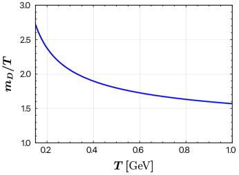
Figure 2: Debye mass in Gribov plasma scaled with temperature is plotted with temperature.

In a thermal medium, the Debye screening mass ($m_{D}$) is an important quantity as this determines how the heavy quark potential gets screened with inter-quark distance. Debye mass $m_{D}$ is defined by taking the static limit of $`$$00$’ component of the gluon self-energy as

$$m_{D}^{2}=\Pi^{00}(p_{0}=0,{\bf{p}}\rightarrow 0).$$ (29)

Within the one-loop order, the Debye screening mass squared can be computed in thermal medium as Bellac (2011)

$$(m_{D}^{T})^{2}=\Big{(}N_{c}+\frac{N_{f}}{2}\Big{)}\frac{g^{2}T^{2}}{3}.$$ (30)

The gluon and ghost loop of the gluon self-energy gets modified in the presence of the Gribov medium. By taking the static limit of $\Pi_{00}^{(a+b+c+d)}(P)$, we get the Debye mass in thermal Gribov plasma. We have plotted the variation of the Debye mass scaled with temperature in fig. 2. The nature of the plot is similar to the Ref. Burnier and Rothkopf (2016); Laine et al. (2020).

V Heavy quark-antiquark potential

The physics of quarkonium state at zero temperature can be explained in terms of non-relativistic potential models, where the masses of heavy quark ($m_{Q}$) are much higher than QCD scale ($\Lambda_{QCD}$), and velocity of the quarks in the bound state is small, $v\ll 1$ Lucha et al. (1991); Brambilla et al. (2005). Therefore, to realise the binding effects in quarkonia, one generally uses the non-relativistic potential models Eichten et al. (1980). In the following subsections, we investigate the effect of the Gribov parameter at finite temperature in the heavy quark-antiquark potential.

V.1 Real part of potential

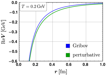
Figure 3: Variation of real part of quarkonium potential with distance for fixed temperature $T=0.2$ GeV.

The real part of the HQ potential gives rise to the Debye screening, and in the non-relativistic limit, it can be determined from the Fourier transform of static gluon propagator as

$$V(r)=g^{2}C_{F}\int\frac{d^{3}p}{(2\pi)^{3}}\,\,\Delta_{00}(p_{0}=0,{p})\,\,e^{i\bf{p}\cdot\mathbf{r}}$$ (31)

For the free case we can write,

$$\Delta^{0}_{00}(p_{0}=0,{p})=-\frac{{p}^{2}}{({p}^{2})^{2}+\gamma_{G}^{4}},$$ (32)

and after the Fourier transform leads to the expression

$$V_{0}(r)=-\frac{C_{F}g^{2}}{4\pi r}\exp\left[-\frac{\gamma_{G}r}{\sqrt{2}}\right]\cos\left(\frac{\gamma_{G}r}{\sqrt{2}}\right).$$ (33)

To investigate the static potential at finite temperature, we can consider a medium effect to this potential due to thermal bath. In a thermal medium, the effective gluon propagator is given by,

$$\Delta_{00}(p_{0}=0,{p}) = -\frac{{p}^{2}}{{p}^{4}+\gamma_{G}^{4}+{p}^{2}\Pi_{L}(p_{0}=0,{p})}.$$ (34)

In this case the heavy-quark potential in coordinate space can be written as

$$V(r) = -g^{2}C_{F}\int\frac{d^{3}p}{(2\pi)^{3}}\,\,e^{i\bf{p}\cdot\mathbf{r}}\,\,\frac{p^{2}}{p^{4}+\gamma_{G}^{4}+p^{2}m_{D}^{2}}$$ (35)

$$= -\frac{g^{2}C_{F}}{(2\pi)^{3}}\int\,\frac{4\pi p^{3}\,dp\,}{p^{4}+\gamma_{G}^{4}+p^{2}m_{D}^{2}}\frac{\sin(p\,r)}{r},$$

where $m_{D}$ is the Debye mass.

When the Gribov parameter $\gamma_{G}=0$, from Eq. (35) we get back the isotropic potential

$$V(r,\gamma_{G}=0) = -g^{2}C_{F}\int\frac{d^{3}p}{(2\pi)^{3}}\,\,e^{i\bf{p}\cdot\mathbf{r}}\,\,\frac{1}{p^{2}+(m^{T}_{D})^{2}}$$ (36)

$$= -\frac{g^{2}C_{F}}{4\pi r}\exp[-{r}/{m^{T}_{D}}],$$

where $m^{T}_{D}$ is the Debye mass for pure thermal case without Gribov.

For the $r\rightarrow 0$ limit, the denominator will be dominated by $p^{2}$ as $p\rightarrow\infty$ and we recover vacuum Coulomb potential

$$V(r\rightarrow 0) = -g^{2}C_{F}\int\frac{d^{3}p}{(2\pi)^{3}}\,\,e^{i\bf{p}\cdot\mathbf{r}}\,\,\frac{1}{p^{2}}$$ (37)

$$= -\frac{g^{2}C_{F}}{4\pi r}.$$

The real part of the potential is shown in fig. 3. We compare the Gribov-modified potential with the pure thermal Coulomb potential. The green line represents the screened potential in the thermal medium, whereas the blue line shows the Gribov result. In the presence of the Gribov parameter, the potential value is less negative than the perturbative case at fixed $r$, indicating more screening. This happens because the Debye mass of Gribov plasma is higher than the pure thermal medium at a fixed temperature.

V.2 Imaginary part of potential

The heavy quark is dissociated at finite temperatures by color screening and Landau damping. The Landau damping part is related to the imaginary part of the gluon self-energy as initially suggested in Ref. Laine et al. (2007). The imaginary part of the in-medium heavy quark potential related to the gluon propagator is written as,

$$\text{Im}\,V(r) =\int\frac{d^{3}p}{(2\pi)^{3}}(e^{i\mathbf{p}\cdot\mathbf{r}}-1)\left(\lim_{p_{0}\to 0}\text{Im}\,\Delta_{00}(P)\right).$$ (38)

The imaginary part of the effective gauge boson propagator can be obtained using the spectral function representation as,

$$\text{Im}\,\Delta_{\mu\nu}(P)=-\pi\left(1+e^{-p_{0}/T}\right)\rho_{\mu\nu}(p_{0},\mathbf{p}),$$ (39)

where $\rho_{\mu\nu}$ is the spectral function, can be obtained from the projection operatores as,

$$\rho^{\mu\nu}(p_{0},\mathbf{p})=\frac{1}{\pi}\frac{e^{p_{0}/T}}{e^{p_{0}/T}-1}\rho_{i}P_{i}^{\mu\nu}.$$ (40)

We can write gluon propagator (20) in the form $\Delta_{\mu\nu}=C_{i}P_{\mu\nu}^{i}$, where $C_{i}$’s are related to the form factors, and $P_{\mu\nu}^{i}$ are the projection operators. Here, $\rho_{i}$ is defined as the imaginary parts of the $i$-th form factor, i.e., $\rho_{i}=\text{Im}\,C_{i}$. In our case we need $\rho^{00}$ which is given by

$$\rho^{00}(p_{0},\mathbf{p})=\frac{1}{\pi}\frac{e^{p_{0}/T}}{e^{p_{0}/T}-1}\rho_{L}P_{i}^{00},$$ (41)

with

$$\rho_{L} = P^{2}\frac{\text{Im}\,\Pi_{L}}{(P^{2}+\gamma_{G}^{4}-P^{2}\,\text{Re}\,\Pi_{L})^{2}}.$$ (42)

The imaginary parts are coming from the Landau damping. The contributions appearing from the self-energy diagrams are finally calculated numerically. In the following subsection, calculations of decay width related to the imaginary part of the potential are presented.

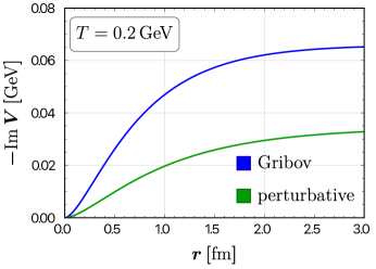
Figure 4: The imaginary part of the quarkonium potential as a function of distance for temperature $T=0.2$ GeV.

The variation of the imaginary part of the potential with separation distance $r$ is shown in fig. 4. The Gribov part is shown with a blue line, whereas the green line denotes the perturbative part. It can be found from the graph that the magnitude of the imaginary part of potential in Gribov is more significant than pure thermal medium at fixed temperature $T$. This behavior indicates more contribution to the Landau damping-induced thermal width in Gribov plasma obtained from the imaginary part of the potential.

V.3 Decay Width

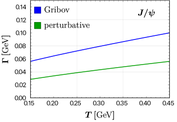
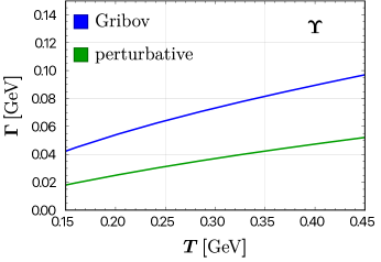
Figure 5: The temperature variation of decay for a charmonium (left panel) and bottomonium (right panel).

In the previous subsection, we obtained the imaginary part of the HQ potential by calculating the imaginary part of gluon self-energy. The imaginary part arises due to the interaction of the particle of momenta order $\sim T$ with space-like gluons, namely, Landau damping. The physics of the finite width emerges from this Landau damping. The imaginary part of the HQ potential plays a crucial role in the dissociation of the HQ-bound state. The formula which gives a good approximation of the decay width ($\Gamma$) of $Q\bar{Q}$ states is written as Thakur et al. (2017),

$$\Gamma(T)=-\int\,|\psi(\mathbf{r})|^{2}\,\text{Im}\,V(\mathbf{r,}T)\,d^{3}\mathbf{r}.$$ (43)

Here we have used the Coulombic wave function for the ground state of hydrogen like atom which is given by

$$\psi(r)=\frac{1}{\sqrt{\pi b_{0}^{3}}}\,e^{-r/b_{0}},$$ (44)

where $b_{0}=\frac{1}{m_{Q}\alpha_{s}}$ is the Bohr radius of the heavy quarkonium system and $m_{Q}$ is the mass of the heavy quark and antiquark. We determine the decay width by substituting the imaginary part of the potential for a given temperature. We evaluate the decay width of the following quarkonia states, $J/\psi$ (the ground state of charmonium, $c\bar{c}$ ) and $\Upsilon$ (bottomonium, $b\bar{b}$).

Fig. 5 displays the variation of decay width with temperature $T$. In this calculation, we have taken the masses of charmonium $(m_{c})$ and bottomonium $(m_{b})$ as $m_{c}=1.275$ GeV and $m_{b}=4.66$ GeV, respectively. The decay width for the charm (left panel) and the bottom (right panel) are shown. As the magnitude of the imaginary part of the potential in Gribov is larger than pure thermal medium, we are getting larger decay width for the case of Gribov plasma. For both the bottom and charm, the decay width is increased in the case of Gribov plasma. The thermal width for $\Upsilon$ is lesser than the $J/\Psi$, as the bottomonium states are smaller in size with larger masses than the charmonium states. But the difference is marginal as we have mainly considered perturbative regions at the high temperature.

VI Discussion

Gribov-improved heavy quark potential and decay width are modified in the presence of a thermal medium. But the confining property is still absent in this scenario. So, in this section, we discuss the heavy quark potential obtained from the localized action and then the medium effect on the potential. The restriction of the integration domain in the functional integral is realized by adding a non-local horizon term to the Faddeev-Popov action Zwanziger (1989b); Canfora et al. (2015). The localization of the horizon non-locality was introduced in Refs. Zwanziger (1989a, b, 1993) by introducing Zwanziger ghost fields, $\{\phi_{\mu}^{ab},\bar{\phi}_{\mu}^{ab}\}$, a pair of commuting fields and $\{\omega_{\mu}^{ab},\bar{\omega}_{\mu}^{ab}\}$, a pair of anti-commuting fields. The Lagrangian is

$$L = L^{\text{YM}}-\bar{c}^{a}\partial^{\mu}D_{\mu}^{ab}c^{b}+\frac{1}{2}\chi^{ab}_{\mu}\partial^{\nu}(D_{\nu}\chi^{\mu})^{ab}+\frac{i}{2}\chi^{ab}_{\mu}\partial^{\nu}(D_{\nu}\xi^{\mu})^{ab}-\frac{i}{2}\xi^{ab}_{\mu}\partial^{\nu}(D_{\nu}\chi^{\mu})^{ab}$$ (45)

$$+ \frac{1}{2}\xi^{ab}_{\mu}\partial^{\nu}(D_{\nu}\xi^{\mu})^{ab}-\bar{\omega}^{ab}_{\mu}\partial^{\nu}(D_{\nu}\omega^{\mu})^{ab}-\frac{1}{\sqrt{2}}gf^{abc}\partial^{\nu}\bar{\omega}_{\mu}^{ae}(D_{\nu}c)^{b}\chi^{ec\,\mu}$$

$$- \frac{i}{\sqrt{2}}gf^{abc}\partial^{\nu}\bar{\omega}_{\mu}^{ae}(D_{\nu}c)^{b}\xi^{ec\,\mu}-i\gamma_{G}^{2}f^{abc}A^{a\,\mu}\xi_{\mu}^{bc}-\frac{1}{2g^{2}}dN\gamma^{4},$$

where $\phi_{\mu}^{ab}=\frac{1}{\sqrt{2}}(\chi_{\mu}^{ab}+i\xi_{\mu}^{ab})$. The authors of Ref. Gracey (2010) have calculated the static potential and discussed the nature of the potential with separation distance. The ghost fields are treated as internal lines in Feynman diagrams. Tree level and one-loop corrections are considered to calculate the static potential. In this work, we have investigated the potential behavior in the presence of a thermal bath. The one loop potential in the Landau gauge is given by (see Ref. Gracey (2010))

$${V}(p)= -\frac{C_{F}g^{2}}{p^{2}}\Bigg{\{}\bigg{[}1-\frac{C_{A}\gamma_{G}^{4}}{\mathbf{p^{2}}^{2}}+\mathcal{O}\bigg{(}\frac{\gamma_{G}^{8}}{(\mathbf{p}^{2})^{4}}\bigg{)}\bigg{]}+\bigg{[}\bigg{(}\frac{31}{9}-\frac{11}{3}\log\left(\frac{\mathbf{p}^{2}}{\Lambda^{2}}\right)\bigg{)}C_{A}$$

$$+\frac{1}{2}\bigg{(}\frac{4}{3}\log\left(\frac{\mathbf{p}^{2}}{\Lambda^{2}}\right)-\frac{20}{9}\bigg{)}N_{f}-\frac{2\pi C_{A}^{3/2}\gamma_{G}^{2}}{\mathbf{p}^{2}}+\bigg{[}\bigg{(}\frac{79}{12}\log\left(\frac{\mathbf{p}^{2}}{\Lambda^{2}}\right)+\frac{9}{8}\log\left(\frac{C_{A}\gamma_{G}^{4}}{(\mathbf{p}^{2})^{2}}\right)-\frac{1315}{72}\bigg{)}C_{A}^{2}$$

$$+\frac{1}{2}\bigg{(}\frac{40}{9}-\frac{8}{3}\log\left(\frac{\mathbf{p}^{2}}{\Lambda^{2}}\right)\bigg{)}N_{f}\bigg{]}\frac{C_{A}\gamma_{G}^{4}}{(\mathbf{p}^{2})^{2}}+\mathcal{O}\bigg{(}\frac{\gamma_{G}^{6}}{(\mathbf{p}^{2})^{3}}\bigg{)}\bigg{]}\frac{g^{2}}{16}+\mathcal{O}\left(g^{4}\right)\Bigg{\}}.$$ (46)

At non-zero temperature, we use an ansatz that the thermal-medium effect enters through the dielectric permittivity $\epsilon(p)$ such as Agotiya et al. (2009); Thakur et al. (2020)

$$\bar{V}(p)=\frac{V(p)}{\epsilon(k)}.$$ (47)

The dielectric permittivity, related to the static limit of $\Pi_{L}(p_{0}=0,p)=m_{D}^{2}$, is given by $\epsilon(p)=(1+\frac{m_{D}^{2}}{p^{2}})$. Finally, using Eq. (47) the in-medium quarkonium potential in real space can be obtained as

$$V(r)= \int\frac{d^{3}p}{(2\pi)^{3}}\,e^{i\mathbb{p}\cdot\mathbb{r}}\,p^{2}\frac{V(p)}{p^{2}+m_{D}^{2}}$$

$$= -\frac{C_{F}g^{2}}{4\pi}\left[4\pi^{2}+\frac{1}{36}(31C_{A}-20N_{f}T_{f})g^{2}\right]\left(\frac{1}{r}+\frac{m_{D}^{2}r}{2}\right)-\frac{1}{72r}C_{F}(11C_{A}-4N_{f}T_{f})g^{2}\alpha_{s}$$

$$\times\left[6[2\gamma_{E}+2\log(\Lambda r)]+3r^{2}m_{D}^{2}\left[-3+2\gamma_{E}+2\log(\Lambda r)\right]+2r^{3}m_{D}^{3}\log\left(\frac{m_{D}}{\Lambda}\right)\right]$$

$$+\frac{\pi r\alpha_{s}\gamma_{G}^{4}}{12m_{D}^{2}}\left[g^{2}m_{D}^{2}(-3C_{A}^{3/2}C_{F}+rm_{D})-8\pi C_{A}C_{F}rT^{2}\gamma_{G}^{2}\right]+\frac{C_{A}C_{F}g^{2}\alpha_{s}\gamma_{G}^{4}r^{2}}{1728m_{D}}\bigg{[}1920-1315C_{A}^{2}$$

$$\left.+81C_{A}^{2}\log\left(\frac{C_{A}\gamma_{G}^{4}}{m_{D}^{4}}\right)\right]-\frac{C_{A}C_{F}g^{2}\alpha_{s}\gamma_{G}^{4}}{288m_{D}^{4}r}\left[(64-79C_{A}^{2})r^{3}m_{D}^{3}+384\sinh(m_{D}r)\right]\log\left(\frac{m_{D}^{2}}{\Lambda^{2}}\right),$$

where $\gamma_{E}=0.57721566...$ is the Euler–Mascheroni constant. Equation (LABEL:eq:aux) is the medium-modified potential of Gribov plasma with auxiliary fields. In the presence of the thermal medium, the linear type potential will not emerge even at one loop contribution as discussed in Ref. Gracey (2010) for vacuum. One should consider higher loop contributions to the HQ potential for improved results.

VII Summary and outlook

In the present theoretical study, the real and imaginary parts of heavy quark complex potential have been computed considering both the perturbative resummation using HTLpt and non-perturbative resummation using Gribov-modified gluon and ghost propagators. Previously HQ potential using Gribov action has been studied at zero temperature. Later, considering one-loop Feynman diagrams via auxiliary fields, HQ potential has been computed. Here we are analyzing the HQ potential at a finite temperature. We first obtained an effective gluon propagator in the presence of the Gribov parameter. The longitudinal and transverse part ($\Pi_{L},\,\Pi_{T}$) of the effective propagator is then obtained from the one-loop gluon self-energy. The gluon self-energy gets the contribution from quark, gluon, and ghost loops. The dependence of the Gribov parameter comes from the gluon and ghost loops. Then we plotted the Debye mass. In our work, an asymptotically high-temperature form of the Gribov parameter $(\gamma_{G})$ has been considered. The real part of the potential is obtained from the Fourier transform of the static gluon propagator. The $Q\bar{Q}$ is more screened in the presence of the Gribov parameter. The imaginary part of the potential and the decay width are evaluated in Gribov plasma. The magnitude of the imaginary part of the potential increases with distance. The width has increased with temperature. We have also discussed the medium effect on the HQ potential in the presence of auxiliary fields at one loop order. As also discussed in Ref. Gracey (2010), the linearly increasing potential in coordinate space is missing even with the additional auxiliary fields. The confining term in the quarkonium potential with Gribov action may appear beyond the leading order of QCD coupling.

VIII Acknowledgment

N.H. is supported in part by the SERB-MATRICS under Grant No. MTR/2021/000939. M.D. and R.G. acknowledge Arghya Mukherjee for helpful discussions.

Appendix A Calculations of self-energy with Gribov parameter

The expression of $J_{1}$ is

$$J_{1} = \int\frac{d^{4}K}{(2\pi)^{4}}\Delta(K)=\int\frac{d^{4}K}{(2\pi)^{4}}\frac{K^{2}}{K^{4}+\gamma_{G}^{4}}$$ (49)

$$= \frac{1}{4\pi^{2}}\sum_{a=\pm}\int_{0}^{\infty}\frac{k^{2}\,dk}{E_{a}(k)}n_{B}(E_{a}(k)),$$

where $E_{a}(k)=\sqrt{k^{2}+ia\gamma_{G}^{2}}$. The expression for $J_{2}$ can be written as

$$J_{2}(P) = \frac{i\gamma_{G}^{2}}{4}\sum_{a,b=\pm 1}\int\frac{d^{4}K}{(2\pi)^{4}}$$ (50)

$$\times \frac{a}{[\omega_{n}^{2}+E_{a}^{2}(k)][(\omega-\omega_{n})^{2}+E_{b}^{2}(|\mathbf{p}-\mathbf{k}|)]}.\ \$$

The structure of $I_{\mu\nu}(P)$ looks like,

$$I_{\mu\nu}(P) = \int\frac{d^{4}K}{(2\pi)^{4}}K_{\mu}K_{\nu}\Delta(K)\Delta(P-K)$$ (51)

$$= \frac{1}{16}\int\frac{d^{4}K}{(2\pi)^{4}}K_{\mu}K_{\nu}\sum_{s,s_{1},a,b=\pm 1}\frac{1}{E_{a}(k)E_{b}(|\mathbf{p}-\mathbf{k}|)}$$

$$\times \frac{s\,s_{1}}{[i\omega_{n}-sE_{a}(k)][i(\omega-\omega_{n})-s_{1}E_{b}(|\mathbf{p}-\mathbf{k}|)]}$$

To calculate the longitudinal $(\Pi_{L})$ and transverse $(\Pi_{T})$ part of the gluon self-energy, we need to calculate $I_{\mu\mu}$ and $I_{44}$. Now,

$$I_{\mu\mu} =\int\frac{d^{4}K}{(2\pi)^{4}}K^{2}\Delta(K)\Delta(P-K)=J_{1}-J_{2},$$ (52)

$$I_{44} =J_{1}-J_{2}-J_{3}.$$ (53)

Now, we calculate $J_{3}$ using HTL approximation. So, one can write

$$J_{3} = \frac{1}{16}\int\frac{d^{3}k}{(2\pi)^{3}}\,k^{2}\sum_{s,s_{1}=\pm 1}\sum_{a,b=\pm}T\sum_{n}\frac{ss_{1}}{E_{a}(k)E_{b}(|{\bf p-k}|)}\frac{1}{[i\omega_{n}-sE_{a}(k)][i(\omega-\omega_{n})-s_{1}E_{b}(|{\bf p-k}|)]}$$

$$= -\frac{1}{16}\int\frac{d^{3}k}{(2\pi)^{3}}\,k^{2}\sum_{s,s_{1}=\pm 1}\sum_{a,b=\pm}\frac{ss_{1}}{E_{a}(k)E_{b}(|{\bf p-k}|)}\frac{1+n_{B}(sE_{a}(k))+n_{B}(s_{1}E_{b}(|{\bf p-k}|))}{i\omega-sE_{a}(k)-s_{1}E_{b}(|{\bf p-k}|)}$$

After analytic continuation and taking the static limit i.e. $i\omega\rightarrow p_{0}=0$ limit, we get,

$$J_{3}(p_{0},\mathbf{p})$$ (55)

$$= \frac{1}{16\pi^{2}}\int\,dk\,k^{4}\sum_{a,b=\pm 1}\frac{n_{B}(E_{a}(k))+n_{B}(E_{b}(k))}{E_{a}(k)E_{b}(k)(E_{a}(k)+E_{b}(k))}+\frac{1}{16\pi^{2}T}\int\,dk\,k^{4}\sum_{a,b=\pm 1}\frac{n_{B}(E_{b}(k))[1+n_{B}(E_{b}(k))]}{E_{a}(k)E_{b}(k)}$$

$$-i\pi\frac{p_{0}}{p}\frac{1}{8T(2\pi)^{2}}\int dk\,k^{4}\sum_{a,b=\pm 1}\frac{n_{B}(E_{b}(k))[1+n_{B}(E_{b}(k))]}{E_{a}(k)E_{b}(k)}.$$ (56)

Similarly for $J_{2}(p_{0},\mathbf{p})$,

$$J_{2}(p_{0},\mathbf{p})$$ (57)

$$=\frac{i\gamma_{G}^{2}}{16\pi^{2}}\int\,dk\,k^{2}\sum_{a,b=\pm 1}\frac{n_{B}(E_{a}(k))+n_{B}(E_{b}(k))}{E_{a}(k)E_{b}(k)(E_{a}(k)+E_{b}(k))}+\frac{i\gamma_{G}^{2}}{16\pi^{2}T}\int\,dk\,k^{2}\sum_{a,b=\pm 1}\frac{n_{B}(E_{b}(k))[1+n_{B}(E_{b}(k))]}{E_{a}(k)E_{b}(k)}$$

$$-i\pi\frac{p_{0}}{p}\frac{i\gamma_{G}^{2}}{8T(2\pi)^{2}}\int dk\,k^{2}\sum_{a,b=\pm 1}\frac{n_{B}(E_{b}(k))[1+n_{B}(E_{b}(k))]}{E_{a}(k)E_{b}(k)}.$$ (58)

Now we compute the expression of $I_{00}^{G}(p_{0},\mathbf{p})$ which appears in ghost loop.

$$I_{00}^{G}(p_{0},\mathbf{p}) = \int\frac{d^{4}K}{(2\pi)^{4}}\frac{k_{0}^{2}}{K^{4}(P-K)^{4}}$$

$$= \lim_{a,b\to 0}\frac{\partial}{\partial a}\frac{\partial}{\partial b}\left[\int\frac{d^{3}k}{(2\pi)^{3}}T\sum_{k_{0}}\frac{k_{0}^{2}}{(k_{0}^{2}+k^{2}+a)((p_{0}-k_{0})^{2}+(p-k)^{2}+b)}\right].$$

After performing Matsubara sum and using the HTL approximation, we get

$$I^{G}_{00}(p_{0},\mathbf{p}) =\int\frac{d^{3}k}{(2\pi)^{3}}\frac{\partial^{2}}{\partial a\partial b}\left[\frac{E_{a}(k)}{E_{b}(k)}\frac{n_{F}(E_{a}(k))+n_{F}(E_{b}(k))}{E_{a}(k)+E_{b}(k)}\right]$$

$$+\frac{\partial^{2}}{\partial a\partial b}\left[\int\frac{k\,dk}{(2\pi)^{2}}E_{a}(k)\left[n_{F}(E_{a}(k))-n_{F}(E_{b}(k))\right]\left(Q_{0}(i\omega_{1}^{ab},p)-Q_{0}(i\omega_{2}^{ab},p)\right)\right]$$

$$+\frac{\partial^{2}}{\partial a\partial b}\left[\int\frac{k\,dk}{(2\pi)^{2}}E_{a}(k)\frac{\partial n_{F}(E_{b}(k))}{\partial k}2\left(Q_{1}(i\omega_{1}^{ab},p)+Q_{1}(i\omega_{2}^{ab},p)\right)\right].$$ (60)

The real part contributes to the Debye mass. We also get the Landau damping from the imaginary part,

$$\lim_{p_{0}\to 0}\text{Im}[I_{00}^{G}(p_{0},p)]=\frac{\pi p_{0}}{p}\int_{0}^{\infty}\frac{dk}{(2\pi)^{2}}\frac{n_{F}(k)}{k^{3}}=\frac{\pi p_{0}}{p}\frac{7\zeta(3)}{8\pi^{2}T^{2}}.$$ (61)

Hence, from Eq. (26) imaginary part of the self-energy from ghost loop looks like

$$\lim_{p_{0}\to 0}\text{Im}[\Pi_{00}^{(c)}(p_{0},p)]=\frac{\pi p_{0}}{p}C_{A}\frac{128^{2}\gamma_{G}^{4}}{32N_{c}^{2}g^{2}T^{2}}7\zeta(3).$$ (62)

References

- Muller (1985) B. Muller, Lect. Notes Phys. 225, 1 (1985).
- Matsui and Satz (1986) T. Matsui and H. Satz, Phys. Lett. B 178, 416 (1986).
- Satz (2007) H. Satz, Nucl. Phys. A 783, 249 (2007), arXiv:hep-ph/0609197 .
- Datta et al. (2004) S. Datta, F. Karsch, P. Petreczky, and I. Wetzorke, Phys. Rev. D 69, 094507 (2004), arXiv:hep-lat/0312037 .
- Ding et al. (2012) H. T. Ding, A. Francis, O. Kaczmarek, F. Karsch, H. Satz, and W. Soeldner, Phys. Rev. D 86, 014509 (2012), arXiv:1204.4945 [hep-lat] .
- Aarts et al. (2013a) G. Aarts, C. Allton, S. Kim, M. P. Lombardo, M. B. Oktay, S. M. Ryan, D. K. Sinclair, and J.-I. Skullerud, JHEP 03, 084 (2013a), arXiv:1210.2903 [hep-lat] .
- Aarts et al. (2013b) G. Aarts, C. Allton, S. Kim, M. P. Lombardo, S. M. Ryan, and J. I. Skullerud, JHEP 12, 064 (2013b), arXiv:1310.5467 [hep-lat] .
- Brambilla et al. (2005) N. Brambilla, A. Pineda, J. Soto, and A. Vairo, Rev. Mod. Phys. 77, 1423 (2005), arXiv:hep-ph/0410047 .
- Bodwin et al. (1995) G. T. Bodwin, E. Braaten, and G. P. Lepage, Phys. Rev. D 51, 1125 (1995), [Erratum: Phys.Rev.D 55, 5853 (1997)], arXiv:hep-ph/9407339 .
- Brambilla et al. (2008) N. Brambilla, J. Ghiglieri, A. Vairo, and P. Petreczky, Phys. Rev. D 78, 014017 (2008), arXiv:0804.0993 [hep-ph] .
- Alberico et al. (2008) W. M. Alberico, A. Beraudo, A. De Pace, and A. Molinari, Phys. Rev. D 77, 017502 (2008), arXiv:0706.2846 [hep-ph] .
- Mocsy (2009) A. Mocsy, Eur. Phys. J. C 61, 705 (2009), arXiv:0811.0337 [hep-ph] .
- Wong (2005) C.-Y. Wong, Phys. Rev. C 72, 034906 (2005), arXiv:hep-ph/0408020 .
- Laine et al. (2007) M. Laine, O. Philipsen, P. Romatschke, and M. Tassler, JHEP 03, 054 (2007), arXiv:hep-ph/0611300 .
- Beraudo et al. (2008) A. Beraudo, J. P. Blaizot, and C. Ratti, Nucl. Phys. A 806, 312 (2008), arXiv:0712.4394 [nucl-th] .
- Brambilla et al. (2013) N. Brambilla, M. A. Escobedo, J. Ghiglieri, and A. Vairo, JHEP 05, 130 (2013), arXiv:1303.6097 [hep-ph] .
- Hayata et al. (2013) T. Hayata, K. Nawa, and T. Hatsuda, Phys. Rev. D 87, 101901 (2013), arXiv:1211.4942 [hep-ph] .
- Albacete et al. (2008) J. L. Albacete, Y. V. Kovchegov, and A. Taliotis, Phys. Rev. D 78, 115007 (2008), arXiv:0807.4747 [hep-th] .
- Rothkopf et al. (2012) A. Rothkopf, T. Hatsuda, and S. Sasaki, Phys. Rev. Lett. 108, 162001 (2012), arXiv:1108.1579 [hep-lat] .
- Bala and Datta (2020) D. Bala and S. Datta, Phys. Rev. D 101, 034507 (2020), arXiv:1909.10548 [hep-lat] .
- Larsen et al. (2020) R. Larsen, S. Meinel, S. Mukherjee, and P. Petreczky, Phys. Lett. B 800, 135119 (2020), arXiv:1910.07374 [hep-lat] .
- Bala et al. (2022) D. Bala, O. Kaczmarek, R. Larsen, S. Mukherjee, G. Parkar, P. Petreczky, A. Rothkopf, and J. H. Weber (HotQCD), Phys. Rev. D 105, 054513 (2022), arXiv:2110.11659 [hep-lat] .
- Shi et al. (2022) S. Shi, K. Zhou, J. Zhao, S. Mukherjee, and P. Zhuang, Phys. Rev. D 105, 014017 (2022), arXiv:2105.07862 [hep-ph] .
- Brambilla et al. (2021) N. Brambilla, M. A. Escobedo, M. Strickland, A. Vairo, P. Vander Griend, and J. H. Weber, JHEP 05, 136 (2021), arXiv:2012.01240 [hep-ph] .
- Akamatsu (2022) Y. Akamatsu, Prog. Part. Nucl. Phys. 123, 103932 (2022), arXiv:2009.10559 [nucl-th] .
- Blaizot et al. (2016) J.-P. Blaizot, D. De Boni, P. Faccioli, and G. Garberoglio, Nucl. Phys. A 946, 49 (2016), arXiv:1503.03857 [nucl-th] .
- Brambilla et al. (2018) N. Brambilla, M. A. Escobedo, J. Soto, and A. Vairo, Phys. Rev. D 97, 074009 (2018), arXiv:1711.04515 [hep-ph] .
- Sharma and Tiwari (2020) R. Sharma and A. Tiwari, Phys. Rev. D 101, 074004 (2020), arXiv:1912.07036 [hep-ph] .
- Escobedo and Soto (2008) M. A. Escobedo and J. Soto, Phys. Rev. A 78, 032520 (2008), arXiv:0804.0691 [hep-ph] .
- Linde (1980) A. D. Linde, Phys. Lett. B 96, 289 (1980).
- Gross et al. (1981) D. J. Gross, R. D. Pisarski, and L. G. Yaffe, Rev. Mod. Phys. 53, 43 (1981).
- Gribov (1978) V. N. Gribov, Nucl. Phys. B 139, 1 (1978).
- Zwanziger (1989a) D. Zwanziger, Nucl. Phys. B 323, 513 (1989a).
- Madni et al. (2023) S. Madni, A. Mukherjee, A. Bandyopadhyay, and N. Haque, Phys. Lett. B 838, 137714 (2023), arXiv:2210.03076 [hep-ph] .
- Bandyopadhyay et al. (2016) A. Bandyopadhyay, N. Haque, M. G. Mustafa, and M. Strickland, Phys. Rev. D 93, 065004 (2016), arXiv:1508.06249 [hep-ph] .
- Su and Tywoniuk (2015) N. Su and K. Tywoniuk, Phys. Rev. Lett. 114, 161601 (2015), arXiv:1409.3203 [hep-ph] .
- Sumit et al. (2023) Sumit, N. Haque, and B. K. Patra, (2023), arXiv:2305.08525 [hep-ph] .
- Sobreiro and Sorella (2005) R. F. Sobreiro and S. P. Sorella, in 13th Jorge Andre Swieca Summer School on Particle and Fields (2005) arXiv:hep-th/0504095 .
- Vandersickel and Zwanziger (2012) N. Vandersickel and D. Zwanziger, Phys. Rept. 520, 175 (2012), arXiv:1202.1491 [hep-th] .
- Dudal et al. (2008) D. Dudal, J. A. Gracey, S. P. Sorella, N. Vandersickel, and H. Verschelde, Phys. Rev. D 78, 065047 (2008), arXiv:0806.4348 [hep-th] .
- Capri et al. (2016) M. A. L. Capri, D. Dudal, D. Fiorentini, M. S. Guimaraes, I. F. Justo, A. D. Pereira, B. W. Mintz, L. F. Palhares, R. F. Sobreiro, and S. P. Sorella, Phys. Rev. D 94, 025035 (2016), arXiv:1605.02610 [hep-th] .
- Gotsman et al. (2021) E. Gotsman, Y. Ivanov, and E. Levin, Phys. Rev. D 103, 096017 (2021), arXiv:2012.14139 [hep-ph] .
- Justo et al. (2022) I. F. Justo, A. D. Pereira, and R. F. Sobreiro, Phys. Rev. D 106, 025015 (2022), arXiv:2206.04103 [hep-th] .
- Canfora et al. (2014) F. Canfora, P. Pais, and P. Salgado-Rebolledo, Eur. Phys. J. C 74, 2855 (2014), arXiv:1311.7074 [hep-th] .
- Gracey (2010) J. A. Gracey, JHEP 02, 009 (2010), arXiv:0909.3411 [hep-th] .
- Golterman et al. (2012) M. Golterman, J. Greensite, S. Peris, and A. P. Szczepaniak, Phys. Rev. D 85, 085016 (2012), arXiv:1201.4590 [hep-th] .
- Wu et al. (2022) W. Wu, G. Huang, J. Zhao, and P. Zhuang, (2022), arXiv:2207.05402 [hep-ph] .
- Fukushima and Su (2013) K. Fukushima and N. Su, Phys. Rev. D 88, 076008 (2013), arXiv:1304.8004 [hep-ph] .
- Bazavov et al. (2012) A. Bazavov, N. Brambilla, X. Garcia i Tormo, P. Petreczky, J. Soto, and A. Vairo, Phys. Rev. D 86, 114031 (2012), arXiv:1205.6155 [hep-ph] .
- Bellac (2011) M. L. Bellac, Thermal Field Theory, Cambridge Monographs on Mathematical Physics (Cambridge University Press, 2011).
- Burnier and Rothkopf (2016) Y. Burnier and A. Rothkopf, Phys. Lett. B 753, 232 (2016), arXiv:1506.08684 [hep-ph] .
- Laine et al. (2020) M. Laine, P. Schicho, and Y. Schröder, Phys. Rev. D 101, 023532 (2020), arXiv:1911.09123 [hep-ph] .
- Lucha et al. (1991) W. Lucha, F. F. Schoberl, and D. Gromes, Phys. Rept. 200, 127 (1991).
- Eichten et al. (1980) E. Eichten, K. Gottfried, T. Kinoshita, K. D. Lane, and T.-M. Yan, Phys. Rev. D 21, 203 (1980).
- Thakur et al. (2017) L. Thakur, N. Haque, and H. Mishra, Phys. Rev. D 95, 036014 (2017), arXiv:1611.04568 [hep-ph] .
- Zwanziger (1989b) D. Zwanziger, Nucl. Phys. B 321, 591 (1989b).
- Canfora et al. (2015) F. E. Canfora, D. Dudal, I. F. Justo, P. Pais, L. Rosa, and D. Vercauteren, Eur. Phys. J. C 75, 326 (2015), arXiv:1505.02287 [hep-th] .
- Zwanziger (1993) D. Zwanziger, Nucl. Phys. B 399, 477 (1993).
- Agotiya et al. (2009) V. Agotiya, V. Chandra, and B. K. Patra, Phys. Rev. C 80, 025210 (2009), arXiv:0808.2699 [hep-ph] .
- Thakur et al. (2020) L. Thakur, N. Haque, and Y. Hirono, JHEP 06, 071 (2020), arXiv:2004.03426 [hep-ph] .