Stochastic Thermodynamics of a Probe in a Fluctuating Correlated Field

Abstract

We develop a framework for the stochastic thermodynamics of a probe coupled to a fluctuating medium with spatio-temporal correlations, described by a scalar field. For a Brownian particle dragged by a harmonic trap through a fluctuating Gaussian field, we show that near criticality the spatially-resolved heat flux develops an unexpected dipolar structure, where on average heat is absorbed in front, and dissipated behind, the particle. Moreover, a perturbative calculation reveals that the dissipated power displays three distinct dynamical regimes depending on the drag velocity.

Stochastic thermodynamics provides powerful tools to investigate the entropic and energetic properties of fluctuating systems coupled to media, even far from equilibrium [1, 2, 3, 4, 5, 6]. A crucial result in this context is the quantitative relation between the time-reversal asymmetry of the system’s fluctuations and the heat dissipated to the environment and associated entropy production [7, 8, 9, 10]. Most of the previous work relied on the assumption that the environment is at all times in equilibrium or in a nonequilibrium steady state, and displays no dynamical spatio-temporal correlations. In various contexts, however, the dynamics crucially hinges on spatio-temporal correlations of the environment — this is the case, e.g., for inclusions in lipid membranes [11, 12, 13, 14], microemulsions [15, 16, 17, 18], or defects in ferromagnetic systems [19, 20, 21, 22, 23, 24]. These correlations become long-ranged and particularly relevant when the environment is close to a critical point, as in the case, e.g., of colloidal particles in binary liquid mixtures [25, 26, 27, 28, 29, 30]. Moreover, the simplified assumption of a structureless environment implies that all the information about local energy and entropy flows occurring within the environment is not taken into account. To overcome this paradigm, there is growing interest in extending concepts from stochastic thermodynamics towards systems with spatially extended correlations, such as pattern-forming many-body systems [31, 32, 33, 34] or critical media [35, 36, 37, 38]. Furthermore, a line of recent works discusses the irreversibility of active many-particle systems described by hydrodynamic field theories [39, 40, 41, 38, 34]. These theoretical advances are driven by state-of-the-art experiments involving optical trapping, ultrafast video-microscopy, or active particles [42, 43, 44, 45, 46].

(a)

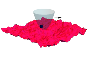
(b)

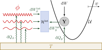
Figure 1: (a) Sketch of a probe particle dragged by a trap with velocity $\mathbf{v}$ through a correlated field (red surface). (b) Cartoon of the particle at position $\mathbf{Y}$, the modes of the field $\phi$ (red waves), and the particle–field interaction (blue box), which can store elastic energy $\mathcal{H}^{\mathrm{int}}$. Particle and field exchange heats ${\mkern 3.0mu\raisebox{-0.6pt}{$\mathchar 22\relax$}\mkern-11.0mu{\rm d}}Q_{y}$ and ${\mkern 3.0mu\raisebox{-0.6pt}{$\mathchar 22\relax$}\mkern-11.0mu{\rm d}}Q_{\phi}$, respectively, with a bath at temperature $T$. An external agent exerts work ${\mkern 3.0mu\raisebox{-0.6pt}{$\mathchar 22\relax$}\mkern-11.0mu{\rm d}}W$ on the particle. Particle and field may exchange energies ${\mkern 3.0mu\raisebox{-0.6pt}{$\mathchar 22\relax$}\mkern-11.0mu{\rm d}}W^{\mathrm{int}}_{y}$ and ${\mkern 3.0mu\raisebox{-0.6pt}{$\mathchar 22\relax$}\mkern-11.0mu{\rm d}}W^{\mathrm{int}}_{\phi}$, respectively, via their interaction. For clarity we do not indicate work exchanges between field modes. Heat fluxes are considered positive when they are supplied to the system.

In this work, we investigate the stochastic thermodynamics of a system consisting of a mesoscopic, externally driven probe coupled to a fluctuating medium. The latter is here represented by a scalar field obeying non-conserved or conserved dynamics [47], and the whole system (probe$+$field) is immersed in a homogeneous heat bath at a fixed temperature ${{T}}$ that induces thermal fluctuations. We provide suitable definitions for the heat, work and entropy exchanges between the probe, the field and the thermal bath, which are consistent with the first and second laws of stochastic thermodynamics. This approach is simpler than addressing a fully microscopic model, while it goes beyond a description based on a generalized Langevin equation (GLE) [48, 49, 50, 51, 52, 52, 53], which may capture temporal, but not spatial correlations of the environment. Notably, our framework is particularly powerful when dealing with a fluctuating medium that is close to a critical point, where one can replace a complex microscopic dynamics with the simplest model belonging to the same universality class [54, 47]. As a fruit of our approach, one can thereby investigate the interplay between the probe, the spatio-temporal correlated field, and the heat bath under the light of stochastic thermodynamics. We illustrate the theory for the minimal yet insightful example of a probe particle dragged by a harmonic trap through a fluctuating Gaussian field. This mimics the setup commonly used to study friction and viscosity in (active) microrheology experiments [55, 56, 57], and is prototypical in stochastic thermodynamics.

The model.— We study a system formed by a mesoscopic probe at $\mathbf{Y}(t)\in\mathbb{R}^{d}$ in $d$ spatial dimensions and a scalar field, whose value at $\mathbf{x}\in\mathbb{R}^{d}$ and time $t$ is denoted by $\phi(\mathbf{x},t)\in\mathbb{R}$. The energy of the system is described by the Hamiltonian

$$\mathcal{H}[\phi,\mathbf{Y},t]=\mathcal{H}_{\phi}[\phi]+\mathcal{H}^{\mathrm{int}}[\phi,\mathbf{Y}]+\mathcal{U}(\mathbf{Y},t),$$ (1)

where $\mathcal{H}_{\phi}$ denotes the energy of the field, $\mathcal{U}$ is an external potential acting only on the probe, and $\mathcal{H}^{\mathrm{int}}$ encodes the interaction between the probe and the field. The probe is assumed to follow the overdamped Langevin equation

$$\gamma_{y}\dot{\mathbf{Y}}=-\gradient_{\mathbf{Y}}\mathcal{H}+\mathbf{F}_{\mathrm{ext}}+\bm{\nu},$$ (2)

where $\mathbf{F}_{\mathrm{ext}}(\mathbf{Y},t)$ accounts for non-conservative external forces. Similarly, the scalar field is assumed to evolve as:

$$\gamma_{\phi}\dot{\phi}=-(-\nabla^{2})^{\mathfrak{a}}\frac{\delta\mathcal{H}}{\delta\phi}+\eta^{(\mathfrak{a})},$$ (3)

with $\mathfrak{a}=0$ or $1$ for locally non-conserved or conserved dynamics [47, 58]. Here $\gamma_{y,\phi}$ are friction coefficients, while $\eta^{(\mathfrak{a})}$ and $\bm{\nu}$ are independent Gaussian white noises satisfying the fluctuation-dissipation relations $\expectationvalue*{\nu_{i}(t)\nu_{j}(t^{\prime})}=2\gamma_{y}{{T}}\delta_{ij}\delta(t-t^{\prime})$ and $\expectationvalue*{\eta^{(\mathfrak{a})}(\mathbf{x},t)\eta^{(\mathfrak{a})}(\mathbf{x}^{\prime},t^{\prime})}=2\gamma_{\phi}{{T}}(-\gradient^{2})^{\mathfrak{a}}\delta^{d}(\mathbf{x}-\mathbf{x}^{\prime})\delta(t-t^{\prime})$, where $\left\langle\ldots\right\rangle$ denotes the average over various noise realizations. Accordingly, in the absence of external driving, i.e., $\mathbf{F}_{\mathrm{ext}}=0$ and time-independent $\mathcal{U}$, the system reaches a state of thermal equilibrium. Figure 1(a) is a sketch of the model with a harmonic external potential $\mathcal{U}$.

First law of stochastic thermodynamics.— To analyze the thermodynamic properties of this system, we generalize ideas from stochastic thermodynamics [2, 1]. For the fluxes of energy and entropy between particle, field and thermal bath sketched in Fig. 1(b), this yields the expressions below (derived in Ref. [59]). First, the only systematic energy input into the system (probe+field) is the work exerted by an external agent on the probe. During a time interval $[t,t+\mathrm{d}t]$, this work is given by

$${\mkern 3.0mu\raisebox{-0.6pt}{$\mathchar 22\relax$}\mkern-11.0mu{\rm d}}W=\frac{\partial\mathcal{U}(\mathbf{Y},t)}{\partial t}\differential t+\mathbf{F}_{\mathrm{ext}}\circ\differential\mathbf{Y},$$ (4)

where ${\mkern 3.0mu\raisebox{-0.6pt}{$\mathchar 22\relax$}\mkern-11.0mu{\rm d}}$ denotes non-exact differentials, and $\circ$ indicates the usage of Stratonovich calculus throughout [1]. The assumption of energy conservation for the probe leads to the first law $\mathrm{d}\mathcal{U}={\mkern 3.0mu\raisebox{-0.6pt}{$\mathchar 22\relax$}\mkern-11.0mu{\rm d}}W+{\mkern 3.0mu\raisebox{-0.6pt}{$\mathchar 22\relax$}\mkern-11.0mu{\rm d}}W^{\mathrm{int}}_{y}+{\mkern 3.0mu\raisebox{-0.6pt}{$\mathchar 22\relax$}\mkern-11.0mu{\rm d}}Q_{y}$, according to which any change $\mathrm{d}\mathcal{U}$ in its potential energy can either be due to ${\mkern 3.0mu\raisebox{-0.6pt}{$\mathchar 22\relax$}\mkern-11.0mu{\rm d}}W$, or caused by the elastic coupling to the field,

$${\mkern 3.0mu\raisebox{-0.6pt}{$\mathchar 22\relax$}\mkern-11.0mu{\rm d}}W^{\mathrm{int}}_{y}:=-\gradient_{\mathbf{Y}}\mathcal{H}^{\mathrm{int}}\circ\mathrm{d}\mathbf{Y}.$$ (5)

The rest must be dissipated into the bath in the form of heat $-{\mkern 3.0mu\raisebox{-0.6pt}{$\mathchar 22\relax$}\mkern-11.0mu{\rm d}}Q_{y}$. From Eqs. (2) to (5) it directly follows that the latter is given by

$${\mkern 3.0mu\raisebox{-0.6pt}{$\mathchar 22\relax$}\mkern-11.0mu{\rm d}}Q_{y}=(-\gamma_{y}\dot{\mathbf{Y}}+\bm{\nu})\circ\mathrm{d}\mathbf{Y},$$ (6)

which is identical to the Sekimoto expression [2] for a single particle in a heat bath (i.e., $\mathcal{H}^{\mathrm{int}}\!=\!0$). Likewise, assuming local energy conservation for the field leads to the first law for the field [59]

$$\mathrm{d}\mathcal{H}_{\phi}=\int\differential[d]{\mathbf{x}}\left[{\mkern 3.0mu\raisebox{-0.6pt}{$\mathchar 22\relax$}\mkern-11.0mu{\rm d}}W^{\mathrm{int}}_{\phi}(\mathbf{x})+{\mkern 3.0mu\raisebox{-0.6pt}{$\mathchar 22\relax$}\mkern-11.0mu{\rm d}}Q_{\phi}(\mathbf{x})\right].$$ (7)

(An analogous, spatially-resolved first law is given in Ref. [59].) Accordingly, all the work done on $\phi$ is either stored in the field configuration $\mathrm{d}\mathcal{H}_{\phi}$ (its “bending”), or dissipated in the form of heat ${\mkern 3.0mu\raisebox{-0.6pt}{$\mathchar 22\relax$}\mkern-11.0mu{\rm d}}Q_{\phi}$. Here,

$${\mkern 3.0mu\raisebox{-0.6pt}{$\mathchar 22\relax$}\mkern-11.0mu{\rm d}}W^{\mathrm{int}}_{\phi}(\mathbf{x}):=-[{\delta\mathcal{H}^{\mathrm{int}}}/{\delta\phi(\mathbf{x})}]\circ\mathrm{d}\phi(\mathbf{x})$$ (8)

is the work locally exerted on the field by the elastic coupling. In general, ${\mkern 3.0mu\raisebox{-0.6pt}{$\mathchar 22\relax$}\mkern-11.0mu{\rm d}}W^{\mathrm{int}}_{y}\neq-\int\differential[d]{\mathbf{x}}{\mkern 3.0mu\raisebox{-0.6pt}{$\mathchar 22\relax$}\mkern-11.0mu{\rm d}}W^{\mathrm{int}}_{\phi}(\mathbf{x})$, because $\mathcal{H}^{\mathrm{int}}$ itself can store energy. From Eqs. 7 and 3 we find that the stochastic heat ${\mkern 3.0mu\raisebox{-0.6pt}{$\mathchar 22\relax$}\mkern-11.0mu{\rm d}}Q_{\phi}$ takes the form

$${\mkern 3.0mu\raisebox{-0.6pt}{$\mathchar 22\relax$}\mkern-11.0mu{\rm d}}Q_{\phi}(\mathbf{x})=\left\{(-\nabla^{2})^{-\mathfrak{a}}\left[\eta^{(\mathfrak{a})}(\mathbf{x})-\gamma_{\phi}\dot{\phi}(\mathbf{x})\right]\right\}\circ\mathrm{d}\phi(\mathbf{x}),$$ (9)

generalizing Sekimoto’s expression [1]. Importantly, ${\mkern 3.0mu\raisebox{-0.6pt}{$\mathchar 22\relax$}\mkern-11.0mu{\rm d}}Q_{\phi}$ is a density (or field) of local heat dissipation. For $\mathfrak{a}=0$, Eq. 9 formally resembles the heat exchange of a single particle. For conserved dynamics ($\mathfrak{a}=1$), the differential operator further introduces terms nonlocal in space.

Second law of stochastic thermodynamics.— Next, we define the irreversibility associated with an individual, joint (probe+field) trajectory $\{\mathbf{Y},\phi\}_{t_{\mathrm{i}}}^{t_{\mathrm{f}}}$ as [1, 40]

$${S}_{\mathrm{tot}}[\{\mathbf{Y},\phi\}_{t_{\mathrm{i}}}^{t_{\mathrm{f}}}]=\ln\frac{\mathcal{P}[\{\mathbf{Y},\phi\}_{t_{\mathrm{i}}}^{t_{\mathrm{f}}}]}{\mathcal{P}^{\mathrm{R}}[\{\mathbf{Y}^{\mathrm{R}},\phi^{\mathrm{R}}\}_{t_{\mathrm{i}}}^{t_{\mathrm{f}}}]}.$$ (10)

Here $\mathcal{P}$ denotes the path probability of the trajectory, starting with the joint probability density $\rho_{\mathbf{Y},\phi}[\mathbf{Y}({t_{\mathrm{i}}}),\phi(\mathbf{x},{t_{\mathrm{i}}})]$, while $\mathcal{P}^{\mathrm{R}}$ denotes the path probability of the corresponding time-reversed process . By construction, the second law $\left\langle{S}_{\mathrm{tot}}\right\rangle\geq 0$ holds [61]. A central result of this manuscript is that the irreversibility ${S}_{\mathrm{tot}}$ defined in Eq. 10 is equivalent to the total thermodynamic entropy production

$${S}_{\mathrm{tot}}=-\frac{Q_{y}}{T}-\int\differential[d]{\mathbf{x}}\frac{Q_{\phi}(\mathbf{x})}{T}+\Delta S_{y,\phi}^{\mathrm{sh}},$$ (11)

with the heat dissipation $Q_{y}$ and $Q_{\phi}$ defined in Eqs. 6 and 9, respectively — indicating the thermodynamic consistency of our framework [59]. Here $\Delta S_{y,\phi}^{\mathrm{sh}}$ denotes the change of the Shannon entropy, $S_{y,\phi}^{\mathrm{sh}}\propto-\ln\rho_{\mathbf{Y},\phi}$.

If the system admits a steady state, then $\expectationvalue*{\mathrm{d}\mathcal{H}^{\mathrm{int}}}$, $\expectationvalue*{\mathrm{d}\mathcal{H}_{\phi}}$, and $\expectationvalue*{\mathrm{d}\mathcal{U}}$ vanish. This simplifies the first laws for probe and field, and implies $\expectationvalue*{\int\differential[d]{\mathbf{x}}{\mkern 3.0mu\raisebox{-0.6pt}{$\mathchar 22\relax$}\mkern-11.0mu{\rm d}}W^{\mathrm{int}}_{\phi}(\mathbf{x})}=-\expectationvalue*{{\mkern 3.0mu\raisebox{-0.6pt}{$\mathchar 22\relax$}\mkern-11.0mu{\rm d}}W^{\mathrm{int}}_{y}}$. Together with the second law and Eq. 11, this implies

$${\left\langle\dot{W}\right\rangle}=-\left\langle\dot{Q}_{y}\right\rangle-{\int\differential[d]{\mathbf{x}}\left\langle\dot{Q}_{\phi}(\mathbf{x})\right\rangle}=T\left\langle\dot{S}_{\mathrm{tot}}\right\rangle\geq 0,$$ (12)

with $\dot{Q}:={\mkern 3.0mu\raisebox{-0.6pt}{$\mathchar 22\relax$}\mkern-11.0mu{\rm d}}Q/\mathrm{d}t$, $\dot{W}:={\mkern 3.0mu\raisebox{-0.6pt}{$\mathchar 22\relax$}\mkern-11.0mu{\rm d}}W/\mathrm{d}t$, and $\dot{S}_{\mathrm{tot}}\simeq{S}_{\mathrm{tot}}/(t_{\mathrm{f}}-t_{\mathrm{i}})$. Thus, in steady states, $\expectationvalue*{\dot{S}_{\mathrm{tot}}}$ is proportional to the average power $\langle\dot{W}\rangle$ injected into the system.

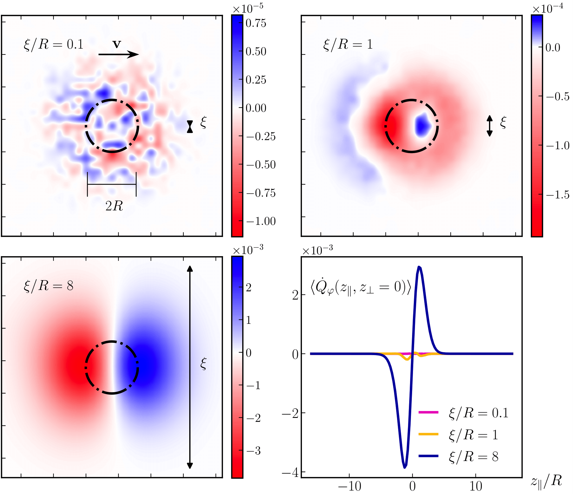
Figure 2: Average local heat dissipation rate $\expectationvalue*{\dot{Q}_{\varphi}(\mathbf{z})}$ by the field into the bath, in a frame comoving at velocity $\mathbf{v}$ with the harmonic trap (see Fig. 1). These results of numerical simulations [59] refer to a Gaussian field in $d=2$ with non-conserved dynamics and, from (a) to (c), increasing values of $\xi/R$, where $\xi$ is the correlation length and $R$ the probe size. The dash-dotted circles indicate the size of the probe. Panel (d) shows $\expectationvalue*{\dot{Q}_{\varphi}(\mathbf{z})}$ along the drag direction $z_{\parallel}$, for $z_{\perp}=0$ and the values of $\xi$ considered in (a–c). We used $L=128$, $\Delta t=10^{-2}$, $\lambda=5$, $v=5$, a Gaussian potential $V$ with variance $R=4$, and set all the other parameters to unity.

Example: Particle dragged through a Gaussian field.— Within this framework, we consider the typical setup [55] in which a probe particle is confined in a harmonic trap of stiffness $\kappa$ moving at constant velocity $\mathbf{v}$. The corresponding potential is $\mathcal{U}(\mathbf{Y},t)=\kappa\left(\mathbf{Y}-\mathbf{v}t\right)^{2}/2$, and the dissipation rate follows from Eq. 4 as

$$\dot{W}=-\kappa\mathbf{v}\cdot\left(\mathbf{Y}-\mathbf{v}t\right).$$ (13)

In the long-time limit, the system reaches a steady state in the comoving reference frame with velocity $\mathbf{v}$. As a minimal model for a near-critical medium — and as the simplest approximation of various complex systems — we consider a Gaussian field with Hamiltonian [47]

$$\mathcal{H}_{\phi}=\frac{1}{2}\int\differential[d]{\mathbf{x}}\left[(\nabla\phi)^{2}+r\phi^{2}\right].$$ (14)

The correlation length $\xi=r^{-1/2}\geq 0$ controls the spatial range of the field correlations at equilibrium, and diverges upon approaching the critical point $r=0$. We model the particle–field interaction, as in demery2010, demery2010-2, demery2011, demerypath, Dean_2011, demery2013,Refs. Ref. [19, 20, 21, 22, 23, 24], by

$$\mathcal{H}_{\text{int}}=-\lambda\int\differential[d]{\mathbf{x}}\phi(\mathbf{x})V(\mathbf{x}-\mathbf{Y}),$$ (15)

where $V(\mathbf{x})\geq 0$ is a rotationally invariant function, with unit spatial integral and rapidly vanishing as $|\mathbf{x}|$ increases beyond the “radius” $R$ of the particle, while $\lambda$ sets the coupling strength. For $\lambda>0$ and at equilibrium, configurations in which the field is enhanced around the particle are energetically favored. We express the particle position in the comoving frame as $\mathbf{Z}\equiv\mathbf{Y}-\mathbf{v}t+\mathbf{v}\gamma_{y}/\kappa$, so that $\mathbf{Z}=0$ is the mean steady-state position for $\lambda=0$. Similarly, we introduce the field $\varphi(\mathbf{z},t)\equiv\phi(\mathbf{z}+\mathbf{v}t-\mathbf{v}\gamma_{y}/\kappa,t)$ in the comoving frame.

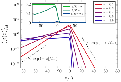
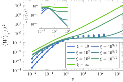
Figure 3: (a) Steady-state expectation value $\langle\varphi(z)\rangle_{\rm st}$ of the field in the comoving frame, for various drag velocities $v>0$, in $d=1$ and with non-conserved dynamics. The shadow $\langle\varphi(z)\rangle_{\rm st}$ flattens upon increasing $v$ (at fixed correlation length $\xi=10$, main plot) or upon decreasing $\xi$ (at fixed $v=5$, inset). $\langle\varphi(z)\rangle_{\rm st}$ decays exponentially upon increasing $|z|$ with different decay lengths $\ell_{\pm}$ in front of or behind the particle — see the main text and Ref. [59]. We used $V_{q}=\exp(-q^{2}R^{2}/2)$ and $R^{2}+{{T}}/\kappa=1$, while the other parameters were set to unity. (b) Additional dissipation rate [see Eq. 21] as a function of $v$, for various values of $\xi$ (with $T=0.1$, while the other parameters were set to one). Symbols correspond to simulations. Inset: scaled correction $-\left\langle Z\right\rangle/\lambda^{2}$ to the average particle position [see Eq. (19)].

Heat dissipation field.— The first thermodynamic quantity we analyze is the spatially resolved heat dissipation $Q_{\varphi}$ in the comoving reference frame [59]. In Fig. 2 we show numerical results for $\left\langle\dot{Q}_{\varphi}\right\rangle$ of a field in $d=2$ with $\mathfrak{a}=0$. For small values of $\xi$ [see panel (a)], we observe that $\left\langle\dot{Q}_{\varphi}\right\rangle$ is essentially negligible (within numerical uncertainties) and displays no discernible spatial structure. In contrast, if $\xi$ reaches the order of the particle size $R$ [panel (b)], regions of average heat dissipation ($\left\langle{\dot{Q}_{\varphi}}\right\rangle<0$) or absorption ($\left\langle{\dot{Q}_{\varphi}}\right\rangle>0$) start developing. Close to criticality, with $\xi\gg R$ [panel (c)], a dissipation dipole forms, with a region of heat absorption in front of the particle, whose spatial extent is approximately given by $\xi$. Hence, surprisingly, in front of the particle the heat bath supplies net energy as if it was coupled to a cooler object. Note that the second law implies $\left\langle{\dot{Q}_{y}}\right\rangle+\int\differential^{d}{\mathbf{x}}\left\langle{\dot{Q}_{\varphi}(\mathbf{x})}\right\rangle<0$, but it does not preclude local heat absorption, i.e., $\left\langle{\dot{Q}_{\varphi}(\mathbf{x})}\right\rangle>0$ for some $\mathbf{x}$. To further elucidate the origin of this effect, below we analytically investigate the statistics of particle and field for various values of $v=|\mathbf{v}|$ and $\xi$, and the dissipated power.

Particle statistics and bending of the field.— We now assume $\lambda$ to be small, and use it as a perturbative parameter [62, 63, 64, 65, 66]. Expressing Eqs. 2 and 3 in terms of $\mathbf{Z}$ and $\varphi$, we first obtain

$$\gamma_{y}\dot{\mathbf{Z}}=-\kappa\mathbf{Z}+\lambda\int\frac{\differential[d]{p}}{(2\pi)^{d}}i\mathbf{p}V_{-p}\varphi_{\mathbf{p}}e^{i\mathbf{p}\cdot\mathbf{Z}}+\bm{\nu},$$ (16)

$$\gamma_{\phi}(\partial_{t}-i\mathbf{p}\cdot\mathbf{v}+\alpha_{p})\varphi_{\mathbf{p}}=\lambda p^{2\mathfrak{a}}V_{p}e^{-i\mathbf{p}\cdot\mathbf{Z}}+\eta_{\mathbf{p}},$$ (17)

where $\alpha_{p}\equiv p^{2\mathfrak{a}}(p^{2}+r)/\gamma_{\phi}$, and $\varphi_{\mathbf{p}}$ is the Fourier transform of $\varphi(\mathbf{x},t)$ . From Eq. 17 we can calculate the mean stationary profile $\left\langle\varphi_{\mathbf{p}}\right\rangle_{\text{st}}$, which is comoving with the particle, and which we call “shadow” [59]. The latter is shown in Fig. 3(a) for a field in $d=1$ with $\mathfrak{a}=0$: the field is strongly bent around the particle, while $\expectationvalue*{\varphi(z)}_{\text{st}}\propto\exp(-|z|/\ell_{\pm})$ for $z\to\pm\infty$, with $\ell_{\pm}=\xi[\sqrt{1+(\xi v\gamma_{\phi}/2)^{2}}\mp(\xi v\gamma_{\phi}/2)]$ [59]. Far from criticality ($\xi\to 0$, see inset), the shadow vanishes, rationalizing the corresponding vanishing of $\expectationvalue*{\dot{Q}_{\varphi}(\mathbf{z})}$ in Fig. 2(a).

Via a perturbative approach, we can investigate the particle fluctuations analytically. The moment generating function $g(\mathbf{q})\equiv\expectationvalue*{\exp(-i\mathbf{q}\cdot\mathbf{Z})}$ of the particle position at the lowest nontrivial order in $\lambda$ reads [59]

$$\ln g(\mathbf{q})=-\frac{q^{2}{{T}}}{2\kappa}+\frac{i\lambda^{2}}{\kappa}\int_{0}^{\infty}\!\frac{\differential{u}}{\sigma^{2}(u)}\int\!\frac{\differential[d]{p}}{(2\pi)^{d}}\frac{\left(\mathbf{p}\cdot\mathbf{v}\right)}{p^{2}+r}|V_{p}|^{2}$$

$$\quad\times G_{\mathbf{p}}(u)e^{-p^{2}\sigma^{2}(u)}\left[1-e^{-\left(\mathbf{p}\cdot\mathbf{q}\right)\sigma^{2}(u)}\right]+\order{\lambda^{4}},$$ (18)

where $\sigma^{2}(u)\equiv{{T}}\left(1-e^{-\kappa u/\gamma_{y}}\right)/\kappa$, and $G_{\mathbf{p}}(u)\equiv\exp[-\alpha_{p}u+i\left(\mathbf{p}\cdot\mathbf{v}\right)u]$. Interestingly, Eq. 18 predicts a non-Gaussian statistics of the particle position. In addition, the variance $\expectationvalue*{Z_{l}Z_{m}}_{c}\propto\delta_{lm}$ changes anisotropically compared to the case $\mathbf{v}=\mathbf{0}$, so that the position distribution is elongated in the direction parallel to $\mathbf{v}$ [68, 59]. Furthermore, $i\nabla_{\mathbf{q}}g|_{\mathbf{q}=\mathbf{0}}$ gives the average displacement

$$\expectationvalue*{\mathbf{Z}}=-\frac{\lambda^{2}}{\kappa}\int\!\frac{\differential[d]{p}}{(2\pi)^{d}}\frac{\mathbf{p}\left(\mathbf{p}\cdot\mathbf{v}\right)}{p^{2}+r}|V_{p}|^{2}\int_{0}^{\infty}\!\differential{u}G_{\mathbf{p}}(u)e^{-p^{2}\sigma^{2}(u)},$$ (19)

which turns out to be directed along $-\mathbf{v}$; hence, the field induces a shift of the probability density of the particle position, which lags behind the average stationary value in the absence of the field [see the inset of Fig. 3(b)]. Such a lag is the footprint of an underlying additional source of dissipation, which we analyze next.

Power fluctuations.— From the moment generating function in Eq. 18, we can access the distribution of the dissipated power. Indeed, rewriting Eq. 13 in terms of $\mathbf{Z}$ gives $\dot{W}=\gamma_{y}v^{2}-\kappa\mathbf{v}\cdot{\mathbf{Z}}$, and thus

$$\ln\expectationvalue{\exp(-i\mu\dot{W})}=-i\mu\gamma_{y}v^{2}+\ln g(-\mu\kappa\mathbf{v}),$$ (20)

encoding all moments of the dissipated power. To study the impact of the field, we focus on the average power

$$\expectationvalue*{\dot{W}}=\gamma_{y}v^{2}-\kappa\mathbf{v}\cdot\expectationvalue*{\mathbf{Z}}\equiv\expectationvalue*{\dot{W}}_{0}+\expectationvalue*{\dot{W}}_{\lambda},$$ (21)

where we identify the dissipation rate in the absence of the field $\expectationvalue*{\dot{W}}_{0}=\gamma_{y}v^{2}\geq 0$, while $\expectationvalue*{\dot{W}}_{\lambda}=-\kappa\mathbf{v}\cdot\left\langle\mathbf{Z}\right\rangle\geq 0$ encodes the additional dissipation due to the field. According to Eq. (12), these are further equal to the entropy production at $\lambda=0$ and $\lambda>0$, i.e., $\expectationvalue*{\dot{W}}_{0}=T\left\langle\dot{S}_{\mathrm{tot}}\right\rangle_{0}$ and $\expectationvalue*{\dot{W}}_{\lambda}=T\left\langle\dot{S}_{\mathrm{tot}}\right\rangle_{\lambda}$, respectively. In Fig. 3(b) we show the perturbative prediction for $\expectationvalue*{\dot{W}}_{\lambda}$ as a function of $v$, and the corresponding numerical data from simulations [59], which are in good agreement. We find that $\expectationvalue*{\dot{W}}_{\lambda}$ generally displays three distinct regimes upon increasing $v$: first, $\absolutevalue{\left\langle Z\right\rangle}$ grows linearly [see Fig. 3(b), inset], so that $\expectationvalue*{\dot{W}}_{\lambda}\propto v^{2}$, as it would be the case for usual Stokes friction. After a crossover, in the second regime $\absolutevalue{\left\langle Z\right\rangle}\propto 1/v$, and therefore $\expectationvalue*{\dot{W}}_{\lambda}$ plateaus at intermediate $v$, which indicates a constant energetic cost associated with the particle–field interaction. Finally, in the third regime, $\absolutevalue{\left\langle Z\right\rangle}$ saturates and thus $\expectationvalue*{\dot{W}}_{\lambda}\propto v$ . We remark that the second and third non-Stokesian regimes cannot be captured by a linear GLE [59].

We present a thorough analysis of these regimes in SM,Refs. Ref. [59], for the case $\mathfrak{a}=0$, and summarize it here. First, by inserting into Eq. 16 the formal solution of Eq. 17 for $\varphi_{\mathbf{p}}(t)$, an effective equation for $\mathbf{Z}(t)$ can be obtained, which is non-Markovian and nonlinear. However, in the limit of small $v$, the field is sufficiently fast to equilibrate around the particle at any instant in time [64, 65]. Conversely, for large $v$, the evolution of the field is so slow that the particle encounters an effectively static field configuration. Accordingly, the first two regimes can be quantitatively captured by adiabatically replacing the field $\varphi_{\mathbf{p}}(t)$ in Eq. 16 with its mean (comoving) profile $\left\langle\varphi_{\mathbf{p}}\right\rangle_{\text{st}}$, i.e., with the shadow shown in Fig. 3(a), resulting in an approximately Markovian evolution of $\mathbf{Z}(t)$. In contrast, at intermediate values of $v$, the timescales of the particle dynamics are comparable with the relaxation time $\tau_{\xi}\simeq\gamma_{\phi}\xi^{2}$ of the field, and the adiabatic approximation is no longer accurate: the particle dynamics within the crossover between the first two regimes is dominated by the memory effects caused by the mutual influence of the particle and the field [59]. Finally, in the third regime, the shadow becomes negligible compared to the (critical) fluctuations of the field, and the particle effectively encounters a rough landscape resulting from them. Notably, as the field approaches criticality ($\xi\to\infty$), the amplitude of its fluctuations diverges [58], and thus the last (non-Stokesian) regime extends to low $v$.

Conclusions.— We developed a thermodynamically consistent framework to study the energetic and entropic flows for a probe in a fluctuating medium with spatio-temporal correlations, modeled here by a scalar field immersed in a heat bath. We showed that the mutual influence of the probe and the correlated environment leads to unusual thermodynamic properties, even for the simple example of a particle dragged by a harmonic trap through a Gaussian field. We showed that, close to criticality, a dipolar structure develops in the local heat dissipation field, with systematic heat absorption in front of the particle, and whose extent is determined by the correlation length $\xi$ of the field. Furthermore, the additional power required to drag the particle in the presence of the field features three regimes with distinct scaling in the drag speed $v$, among which are two non-Stokesian regimes — a feature that cannot be captured by a linear GLE. Far from criticality ($\xi\to 0$), the medium is only weakly correlated, and indeed both the heat dipole and the additional dissipation vanish. The framework developed here can be readily applied to study more complex scenarios, e.g., non-quadratic Hamiltonians, or extended to systems of multiple particles in a common correlated (active) environment. Moreover, it would be interesting to explore these phenomena in, e.g., soft-matter experiments within critical or active media [42].

in 1,…,21 See pages \x, of supplemental.pdf