Learning Safety Constraints from Demonstrations with Unknown Rewards

Abstract

We propose Convex Constraint Learning for Reinforcement Learning (CoCoRL), a novel approach for inferring shared constraints in a Constrained Markov Decision Process (CMDP) from a set of safe demonstrations with possibly different reward functions. While previous work is limited to demonstrations with known rewards or fully known environment dynamics, CoCoRL can learn constraints from demonstrations with different unknown rewards without knowledge of the environment dynamics. CoCoRL constructs a convex safe set based on demonstrations, which provably guarantees safety even for potentially sub-optimal (but safe) demonstrations. For near-optimal demonstrations, CoCoRL converges to the true safe set with no policy regret. We evaluate CoCoRL in tabular environments and a continuous driving simulation with multiple constraints. CoCoRL learns constraints that lead to safe driving behavior and that can be transferred to different tasks and environments. In contrast, alternative methods based on Inverse Reinforcement Learning (IRL) often exhibit poor performance and learn unsafe policies.

1 Introduction

Constrained Markov Decision Processes (CMDPs) integrate safety constraints with reward maximization in reinforcement learning (RL). However, similar to reward functions, it can be difficult to specify constraint functions manually (Krakovna et al., 2020). To tackle this issue, recent work proposes learning models of the constraints (e.g., Scobee and Sastry, 2020; Malik et al., 2021) analogously to reward models (Leike et al., 2018). However, existing approaches to constraint inference rely on demonstrations with known reward functions, which is often unrealistic in real-world applications.

For instance, consider the domain of autonomous driving (Figure 1), where specifying rewards/constraints is particularly difficult (Knox et al., 2023). We can gather diverse human driving trajectories that satisfy shared constraints, such as keeping an appropriate distance to other cars and avoiding crashes. But the trajectories will usually have different (unknown) routes or driving style preferences, which we can model as different reward functions. In such scenarios, we aim to infer constraints from demonstrations with shared constraints but unknown rewards.

Contributions.

In this paper: (1) we introduce the problem of inferring constraints in CMDPs from demonstrations with unknown rewards (Section 3.1); (2) we introduce Convex Constraint Learning for Reinforcement Learning (CoCoRL), a novel method for addressing this problem (Section 4); (3) we prove that CoCoRL guarantees safety (Section 4.1), and, for (approximately) optimal demonstrations, asymptotic optimality (Section 4.2), while IRL provably cannot guarantee safety (Section 3.2); and, (4) we conduct comprehensive empirical evaluations of CoCoRL in tabular environments and a continuous driving task with multiple constraints (Section 6). CoCoRL learns constraints that lead to safe driving behavior and that can be transferred across different tasks and environments. In contrast, alternative IRL-based methods often perform poorly and lack safety guarantees.

Overall, our theoretical and empirical results illustrate the potential of CoCoRL for constraint inference and the advantage of employing CMDPs with inferred constraints instead of relying on MDPs with IRL in safety-critical applications.

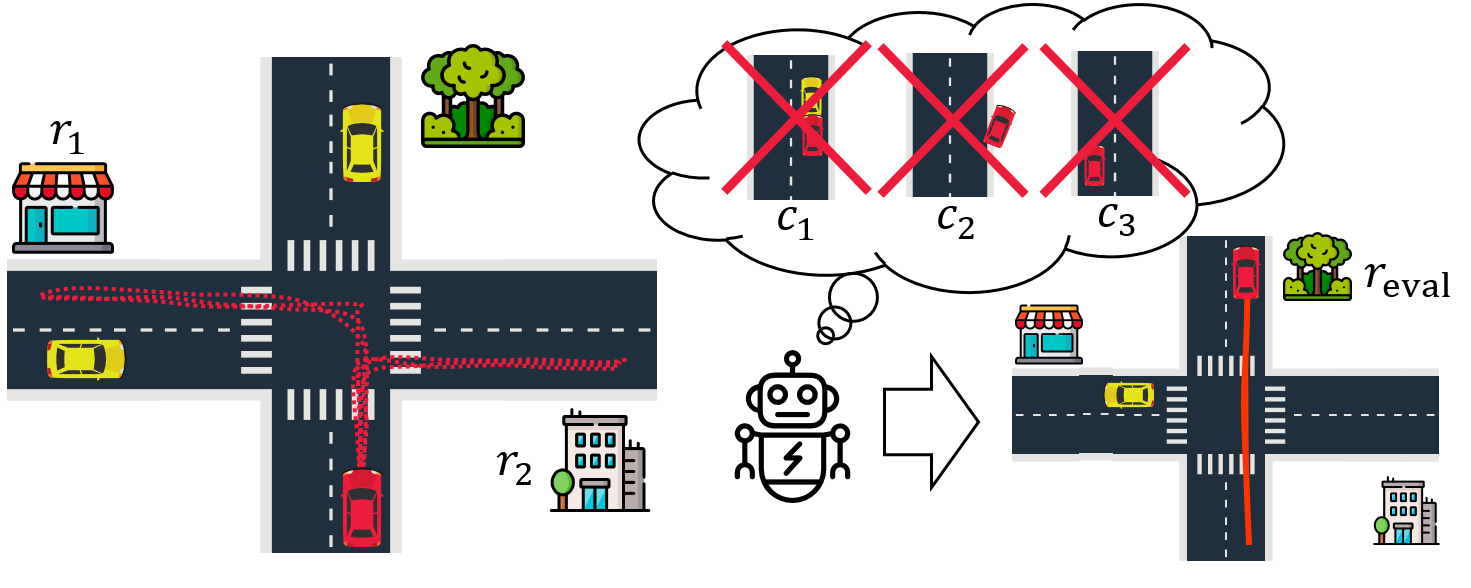
Figure 1: CoCoRL can, for example, learn safe driving behavior from diverse driving trajectories with different unknown goals. It infers constraints $c_{1},c_{2},c_{3}$ describing desirable driving behavior from demonstrations without knowledge of the specific reward functions $r_{1},r_{2}$. These inferred constraints allow to optimize for a new reward function $r_{\text{eval}}$, ensuring safe driving behavior even in new situations for which matching demonstrations are unavailable.

2 Background

Markov Decision Processes (MDPs).

A (infinite-horizon, discounted) MDP (Puterman, 1990) is a tuple $(S,A,P,\mu_{0},\gamma,r)$, where $S$ is the state space, $A$ the action space, $P:S\times A\times S\to[0,1]$ the transition model, $\mu_{0}:S\to[0,1]$ the initial state distribution, $\gamma\in(0,1)$ the discount factor, and $r:S\times A\to[0,1]$ the reward function. An agent starts in an initial state $s\sim\mu_{0}$, then takes actions sampled from a policy $a\sim\pi(a|s)$ that lead to a next state according to the transitions $P(s^{\prime}|s,a)$. The agent aims to maximize the expected discounted return $G_{r}(\pi)=\mathbb{E}_{P,\pi}\left[\sum_{t=0}^{\infty}\gamma^{t}r(s_{t},a_{t})\right]$.

We often use the (discounted) occupancy measure $\mu_{\pi}(s,a)=\mathbb{E}_{P,\pi}\left[\sum_{t=0}^{\infty}\gamma^{t}\mathds{1}_{\{s_{t}=s,a_{t}=a\}}\right]$. For finite state and action spaces, the return is linear in $\mu_{\pi}$, i.e., $G_{r}(\pi)=\sum_{s,a}\mu_{\pi}(s,a)r(s,a)$.

Constrained MDPs (CMDPs).

A CMDP (Altman, 1999) extends an MDP with a set of cost functions $c_{1},\dots,c_{n}$ defined similar to the reward function as $c_{j}:S\times A\to[0,1]$ and thresholds $\xi_{1},\dots,\xi_{n}$. The agent’s goal is to maximize $G_{r}(\pi)$ under constraints on the expected discounted cumulative costs $J_{j}(\pi)=\mathbb{E}_{P,\pi}\left[\sum_{t=0}^{\infty}\gamma^{t}c_{j}(s_{t},a_{t})\right]$. In particular, a feasible policy must satisfy $J_{j}(\pi)\leq\xi_{j}$ for all $j$. Again, we can write the cumulative costs as $J_{j}(\pi)=\sum_{s,a}\mu_{\pi}(s,a)c_{j}(s,a)$.

Inverse Reinforcement Learning (IRL).

IRL aims to recover an MDP’s reward function from expert demonstrations, ensuring the demonstrations are optimal under the identified reward function. It seeks a reward function where the optimal policy aligns with the expert demonstrations’ feature expectations (Abbeel and Ng, 2004). Since the IRL problem is underspecified, algorithms differ in selecting a unique solution, with popular approaches including maximum margin IRL (Ng et al., 2000) and maximum (causal) entropy IRL (Ziebart et al., 2008).

3 Inferring Constraints With Unknown Rewards

In this section, we introduce the problem of inferring constraints from demonstrations in a CMDP. Then, we discuss why naive solutions based on IRL cannot solve this problem.

3.1 Problem Setup

We consider an infinite-horizon discounted CMDP without reward function and cost functions, denoted by $(S,A,P,\mu_{0},\gamma)$. We have access to demonstrations from $k$ safe policies $\mathcal{D}=\{\pi_{1}^{*},\dots,\pi_{k}^{*}\}$, that have $k$ unknown reward functions $r_{1},\dots,r_{k}$, but share the same constraints defined by unknown cost functions $c_{1},\dots,c_{n}$ and thresholds $\xi_{1},\dots,\xi_{n}$. We assume policy $\pi_{i}^{*}$ is safe in the CMDP $(S,A,P,\mu_{0},\gamma,r_{i},\{c_{j}\}_{j=1}^{n},\{\xi_{j}\}_{j=1}^{n})$. Generally, we assume policy $\pi_{i}^{*}$ optimizes for reward $r_{i}$, but it does not need to be optimal.

In our driving example (Figure 1), the rewards of the demonstrations can correspond to different routes and driver preferences, whereas the shared constraints describe driving rules and safety-critical behaviors, such as maintaining an appropriate distance to other cars or staying in the correct lane.

We assume that reward and cost functions are defined on a $d$-dimensional feature space, represented by $\mathbf{f}:S\times A\to[0,1]^{d}$. Instead of having full policies, we have access to their discounted feature expectations (slightly overloading notation) defined as $\mathbf{f}(\pi)=\mathbb{E}_{P,\pi}[\sum_{t=0}^{\infty}\gamma^{t}\mathbf{f}(s_{t},a_{t})]$. The reward and cost functions linear in the feature space, given by $r_{i}(s,a)=\theta_{i}^{T}\mathbf{f}(s,a)$ and $c_{j}(s,a)=\phi_{j}^{T}\mathbf{f}(s,a)$, where $\theta_{i}\in\mathbb{R}^{d}$ and $\phi_{j}\in\mathbb{R}^{d}$ are the respective parameter vectors. For now, we assume we know the exact feature expectations of the demonstrations. In Section 4.3, we discuss sample-based estimation.

Importantly, in the case of a finite state and action space, assuming a feature space is w.l.o.g., because we can use the state-action occupancy measure $\mu_{\pi}(s,a)$ as features. Specifically, we can define $\mathbf{f}(s,a)=(\mathds{1}_{\{s=s_{1},a_{1}\}},\mathds{1}_{\{s=s_{1},a_{2}\}},\dots)$ as an indicator vector with dimension $d=|S||A|$. Then, $\mathbf{f}(\pi)\in\mathbb{R}^{|S||A|}$ is a vector that contains the state-action occupancy values $\mu_{\pi}$, and we have $G_{r}(\pi)=\theta^{T}\mathbf{f}(\pi)=\sum_{s,a}r(s,a)\mu_{\pi}(s,a)$, i.e., the reward parameter $\theta$ is a vector of the state-action rewards. Similarly, the constraint parameters $\phi_{j}$ are vectors of state-action costs $c_{j}$.

For evaluation, we receive a new reward function $r_{\text{eval}}$ and aim to find an optimal policy for the CMDP $(S,A,P,\mu_{0},\gamma,r_{\text{eval}},\{c_{j}\}_{j=1}^{n},\{\xi_{j}\}_{j=1}^{n})$ where the constraints are unknown. Our goal is to ensure safety while achieving a good reward under $r_{\text{eval}}$.

3.2 Limitation of IRL in CMDPs

Initially, we might disregard the CMDP nature of the problem and try to apply standard IRL methods to infer a reward from demonstrations. This approach poses at least two key problems: (1) IRL cannot guarantee safety, and (2) it is unclear how to learn a transferable representation of the constraints.

To elaborate, let us first assume we have a single expert demonstration from a CMDP and apply IRL to infer a reward function, assuming no constraints. Unfortunately, we can show that, in some CMDPs, all reward functions obtained through IRL can yield unsafe optimal policies.

Proposition 1 (IRL can be unsafe).

There are CMDPs $\mathcal{C}=(S,A,P,\mu_{0},\gamma,r,\{c_{j}\}_{j=1}^{n},\{\xi_{j}\}_{j=1}^{n})$ such that for any optimal policy $\pi^{*}$ in $\mathcal{C}$ and any reward function $r_{\text{IRL}}$ that could be returned by an IRL algorithm, the resulting MDP $(S,A,P,\mu_{0},\gamma,r_{\text{IRL}})$ has optimal policies that are unsafe in $\mathcal{C}$.

This follows because CMDPs can have only stochastic optimal policies, whereas MDPs always have a deterministic optimal policy (Puterman, 1990; Altman, 1999). See Appendix A for a full proof of this and other theoretical results in this paper.

Furthermore, even if we manage to learn a reward function that represents the constraints, it remains unclear how to transfer it to a new task represented by the reward function $r_{\text{eval}}$. One potential approach is to model the constraints as a shared reward penalty. Unfortunately, it turns out that learning this shared penalty can be infeasible, even when the rewards are known.

Proposition 2.

Let $\mathcal{C}=(S,A,P,\mu_{0},\gamma,\{c_{j}\}_{j=1}^{n},\{\xi_{j}\}_{j=1}^{n})$ be a CMDP without reward. Let $r_{1},r_{2}$ be two reward functions and $\pi_{1}^{*}$ and $\pi_{2}^{*}$ corresponding optimal policies in $\mathcal{C}\cup\{r_{1}\}$ and $\mathcal{C}\cup\{r_{2}\}$. Let $\mathcal{M}=(S,A,P,\mu_{0},\gamma)$ be the corresponding MDP without reward. Without additional assumptions, we cannot guarantee the existence of a function $\hat{c}:S\times A\to\mathbb{R}$ such that $\pi_{1}^{*}$ is optimal in the MDP $\mathcal{M}\cup\{r_{1}+\hat{c}\}$ and $\pi_{2}^{*}$ is optimal in the MDP $\mathcal{M}\cup\{r_{2}+\hat{c}\}$.

Similar to Proposition 1, this result stems from the fundamental difference between MDPs and CMDPs. The main challenge is to appropriately scale the reward penalty $\hat{c}$ for a specific reward function. While it is always possible to find a suitable $\hat{c}$ to describe a single expert policy with a single known reward function, the situation becomes more complex when dealing with multiple expert policies $\pi_{1}^{*},\pi_{2}^{*}$ and reward functions $r_{1},r_{2}$. In such cases, differently scaled penalties may be required, and the problem of learning a shared $\hat{c}$ can be infeasible. These findings strongly suggest that IRL is not a suitable approach for learning from demonstrations from a CMDP. Our empirical findings in Section 6 confirm this.

4 Convex Constraint Learning for Reinforcement Learning (CoCoRL)

We are now ready to introduce the CoCoRL algorithm. We construct the full algorithm step-by-step: (1) we introduce the key idea of using convexity to construct provably conservative safe set (Section 4.1); (2) we establish convergence results under (approximately) optimal demonstrations (Section 4.2); (3) we introduce several approaches for using estimated feature expectations (Section 4.3); and, (4), we discuss practical considerations for implementing CoCoRL (Section 4.4).

Importantly, when constructing the conservative safe set, we only require access to safe demonstrations. For convergence, we make certain optimality assumptions, either exact optimality or Boltzmann-rationality. Appendix A contains all omitted proofs.

4.1 Constructing a Convex Safe Set

Let the true safe set $\mathcal{F}=\{\pi|\forall j:J_{j}(\pi)\leq\xi_{j}\}$ be the set of all policies that satisfy the constraints. CoCoRL is based on the key observation that $\mathcal{F}$ is convex.

Lemma 1.

For any CMDP, suppose $\pi_{1},\pi_{2}\in\mathcal{F}=\mathcal{F}=\{\pi|\forall j:J_{j}(\pi)\leq\xi_{j}\}$, and let $\bar{\pi}_{12}$ be a policy such that $\mathbf{f}(\bar{\pi}_{12})=\lambda\mathbf{f}(\pi_{1})+(1-\lambda)\mathbf{f}(\pi_{2})$ with $\lambda\in[0,1]$. Then $\bar{\pi}_{12}\in\mathcal{F}$.

$\pi_{1},\pi_{2}\in\mathcal{F}$ means for any $j$, we have $J_{j}(\pi_{1})\leq\xi_{j}$ and $J_{j}(\pi_{2})\leq\xi_{j}$. Then, also for any $j$, we have $J_{j}(\bar{\pi}_{12})=\phi_{j}^{T}\mathbf{f}(\bar{\pi}_{12})=\lambda\phi_{j}^{T}\mathbf{f}(\pi_{1})+(1-\lambda)\phi_{j}^{T}\mathbf{f}(\pi_{2})\leq\xi_{j}$. Thus, $\bar{\pi}_{12}\in\mathcal{F}$.

We know that all demonstrations are safe in the original CMDP and convex combinations of their feature expectations are safe. This insight leads us to a natural approach for constructing a conservative safe set: create the convex hull of the feature expectations of the demonstrations, i.e.,

$$\mathcal{S}=\mathtt{conv}(\mathcal{D})\coloneqq\{\mathbf{x}=\sum_{i=1}^{k}\lambda_{i}\mathbf{f}(\pi^{*}_{i})|\lambda_{i}\geq 0\text{ and }\sum_{i}\lambda_{i}=1\}.$$

To simplify notation, we will sometimes write $\pi\in\mathcal{S}$ to mean $\mathbf{f}(\pi)\in\mathcal{S}$. As $\mathbf{f}$ is fixed, this notation is unambiguous. Thanks to the convexity of $\mathcal{F}$, we can now guarantee safety for all policies $\pi\in\mathcal{S}$.

Theorem 1 (Estimated safe set).

Any policy $\pi\in\mathcal{S}$ is safe, i.e., $\pi\in\mathcal{F}$.

Our demonstrations $\pi_{1}^{*},\dots,\pi_{k}^{*}$ are all in the true safe set $\mathcal{F}$, and any $\pi\in\mathcal{S}$ is a convex combination of them. Given that $\mathcal{F}$ is convex (Lemma 1), we have $\mathcal{S}\subseteq\mathcal{F}$. During evaluation, we are given a new reward $r_{\text{eval}}$, and we want to find $\pi^{*}\in\mathop{\mathrm{missing}}{argmax}_{\pi\in\mathcal{S}}G_{r_{\text{eval}}}(\pi)$. Conveniently, we can reduce this problem to solving a new CMDP with identical dynamics. Specifically, we can find a set of linear cost functions parameterized by $\hat{\phi}_{1},\dots,\hat{\phi}_{m}$ and thresholds $\hat{\xi}_{1},\dots,\hat{\xi}_{m}$, such that $\mathcal{S}=\{x|\hat{\phi}_{j}^{T}x\leq\hat{\xi}_{j}\text{ for all }j\}$. This result follows from standard convex analysis: $\mathcal{S}$ is a convex polyhedron, which is the solution to a set of linear equations. The task of constructing a convex hull from a set of points and identifying the linear equations is a well-studied problem in polyhedral combinatorics (e.g., Pulleyblank, 1983).

Consequently, we can optimize within our safe set $\mathcal{S}$ by identifying and solving an “inferred” CMDP.

Theorem 2 (Inferred CMDP).

We can find cost functions and thresholds such that for any reward function $r_{\text{eval}}$, solving the inferred CMDP $(S,A,P,\mu_{0},\gamma,r_{\text{eval}},\{\hat{c}_{j}\}_{j=1}^{m},\{\hat{\xi}_{j}\}_{j=1}^{m})$ is equivalent to solving $\pi^{*}\in\mathop{\mathrm{missing}}{argmax}_{\pi\in\mathcal{S}}G_{{r}_{\text{eval}}}(\pi)$. Consequently, if an optimal policy for the true CMDP is in $\mathcal{S}$, solving the inferred CMDP will find an optimal policy for the true CMDP.

Note that the number of inferred constraints $m$ is not necessarily equal to the number of true constraints $n$, but we do not assume to know $n$. It immediately follows from Theorem 2 that our safe set is worst-case optimal because, without additional assumptions, we cannot dismiss the possibility that the true CMDP coincides with our inferred CMDP.

Corollary 1 ($\mathcal{S}$ is maximal).

If $\pi\notin\mathcal{S}$, there exist $r_{1},\dots,r_{k}$ and $c_{1},\dots,c_{n}$, such that the expert policies $\pi^{*}_{1},\dots,\pi^{*}_{k}$ are optimal in the CMDPs $(S,A,P,\mu_{0},\gamma,r_{i},\{c_{j}\}_{j=1}^{n},\{\xi_{j}\}_{j=1}^{n})$, but $\pi\notin\mathcal{F}$.

In essence, $\mathcal{S}$ is the largest set we can choose while ensuring safety.

4.2 Convergence for (Approximately) Optimal Demonstrations

So far, we studied the safety of CoCoRL. In this section, we establish its convergence to optimality under two conditions: (1) when the safe demonstrations are exactly optimal, and (2) when they are approximately optimal according to a Boltzmann model.

Given a new reward function $r_{\text{eval}}$, we focus on comparing our safe solution $\max_{\pi\in\mathcal{S}}G_{r}(\pi)$ to the optimal safe solution $\max_{\pi\in\mathcal{F}}G_{r}(\pi)$. In particular, we define the policy regret

$$\mathcal{R}(r,\mathcal{S})=\max_{\pi\in\mathcal{F}}G_{r}(\pi)-\max_{\pi\in\mathcal{S}}G_{r}(\pi).$$

Let us assume the reward functions of the demonstrations and the reward functions during evaluation follow the same distribution $P(r)$. After observing $k$ demonstrations, we construct the safe set $\mathcal{S}_{k}$, and consider the expectation $\mathbb{E}_{r}[\mathcal{R}(r,\mathcal{S}_{k})]$ under the reward distribution. To begin with, let us consider exactly optimal demonstrations.

Assumption 1 (Exact optimality).

Each $\pi_{i}^{*}$ is optimal in the CMDP $(S,A,P,\mu_{0},\gamma,r_{i},\{c_{j}\}_{j},\{\xi_{j}\}_{j})$.

Theorem 3 (Convergence, exact optimality).

Under Assumption 1, for any $\delta>0$, after $k\geq\log(\delta/f_{v}(d,n))/\log(1-\delta/f_{v}(d,n))$, we have $P(\mathcal{R}(r,\mathcal{S}_{k})>0)\leq\delta$, where $f_{v}(d,n)$ is an upper bound on the number of vertices of the true safe set. In particular, $\lim_{k\to\infty}\mathbb{E}_{r}\left[\mathcal{R}(r,\mathcal{S}_{k})\right]=0$.

Due to both the true safe set and the estimated safe set being convex polyhedra, we have a finite hypothesis class consisting of all convex polyhedra with vertices that are a subset of the true safe set’s vertices. The proof builds on the insight that all vertices supported by the distribution induced by $P(r)$ will eventually be observed, while unsupported vertices do not contribute to the regret. The number of vertices is typically on the order $f_{v}(d,n)\in\mathcal{O}(n^{\lfloor d/2\rfloor})$. A tighter bound is given by the McMullen upper bound theorem (McMullen, 1970).

In practical settings, it is unrealistic to assume perfectly optimal demonstrations. Thus, we relax this assumption and consider the case where demonstrations are only approximately optimal.

Assumption 2 (Boltzmann-rationality).

We observe demonstrations following a Boltzmann policy distribution $\pi_{i}^{*}\sim\exp\left(\beta G_{r_{i}}(\pi)\right)\mathds{1}_{\{J_{1}(\pi)\leq\xi_{1},\dots,J_{n}(\pi)\leq\xi_{n}\}}/Z_{i}$, where $G_{r_{i}}(\pi)$ is the expected return computed w.r.t. the reward function $r_{i}$, and $Z_{i}$ is a normalization constant.

Note that Theorem 1 and Corollary 1 still hold under Assumption 2, as they only depend on all demonstrations being safe. Also, we can still establish asymptotic optimality.

Theorem 4 (Convergence, Boltzmann-rationality).

Under Assumption 2, for any $\delta>0$, after $k\geq\log(\delta/f_{v}(d,n))/\log(1-\exp(-\beta d/(1-\gamma)))$, we have $P(\mathcal{R}(r,\mathcal{S}_{k})>0)\leq\delta$, where $f_{v}(d,n)$ is an upper bound on the number of vertices of the true safe set. In particular, $\lim_{k\to\infty}\mathbb{E}_{r}\left[\mathcal{R}(r,\mathcal{S}_{k})\right]=0$.

This result relies on the Boltzmann distribution having a fixed lower bound over the bounded set of policy features. By enumerating the vertices of the true safe set, we can establish an upper bound on the probability of the “bad event” where a vertex is not adequately covered by the set of $k$ demonstrations. This shows how the regret must decrease as $k$ increases.

4.3 Estimating Feature Expectations

So far, we assumed access to the true feature expectations of the demonstrations $\mathbf{f}(\pi_{i}^{*})$. However, in practice, we often rely on samples from the environment to estimate the feature expectations. Given $n_{\text{traj}}$ samples from policy $\pi_{i}^{*}$, a natural way to estimate the feature expectations is by taking the sample mean: $\hat{\mathbf{f}}(\pi_{i}^{*})=\frac{1}{n_{\text{traj}}}\sum_{j=1}^{n_{\text{traj}}}\mathbf{f}(\tau_{j}^{i})$, where $\mathbf{f}(\tau_{j}^{i})=\sum_{t=0}^{\infty}\gamma^{t}\mathbf{f}(s_{t},a_{t})$ and $\tau_{j}^{i}=(s_{0},a_{0},s_{1},a_{1},\dots)$ represents a trajectory from rolling out $\pi_{i}^{*}$ in the environment. This estimate is unbiased, i.e., $\mathbb{E}[\hat{\mathbf{f}}(\pi_{i}^{*})]=\mathbf{f}(\pi_{i}^{*})$, and we can use standard concentration inequalities to measure its confidence. For instance, by using McDiarmid’s inequality, we can ensure $\epsilon$-safety when using the estimated feature expectations.

Theorem 5 ($\epsilon$-safety with estimated feature expectations.).

Suppose we estimate the feature expectations of each policy $\pi_{i}^{*}$ using at least $n_{\text{traj}}>d\log(nk/\delta)/(2\epsilon^{2}(1-\gamma))$ samples, and construct the estimated safe set $\hat{\mathcal{S}}=\mathtt{conv}(\hat{\mathbf{f}}(\pi_{1}^{*}),\dots,\hat{\mathbf{f}}(\pi_{k}^{*}))$. Then, we have $P(\max_{j}(J_{j}(\pi)-\xi_{j})>\epsilon|\pi\in\hat{\mathcal{S}})<\delta$.

We can extend our analysis to derive convergence bounds for exactly optimal or Boltzmann-rational demonstrations, similar to Theorem 3 and Theorem 4. The exact bounds are provided in Section A.4. Importantly, we no regret asymptotically: $\lim_{\min(k,n_{\text{traj}})\to\infty}\mathbb{E}_{r}[\mathcal{R}(r,\mathcal{S}_{k})]=0$, in both cases.

Alternatively, we can leverage confidence sets around $\hat{\mathbf{f}}(\pi_{i}^{*})$ to construct a conservative safe set. This approach guarantees exact safety and convergence as long as the confidence intervals shrink. However, it involves constructing a guaranteed hull (Sember, 2011), which can be computationally more expensive than constructing a simple convex hull. The guaranteed hull can also be overly conservative in practice. See Appendix B for a detailed discussion.

Crucially, CoCoRL can be applied in environments with continuous state and action spaces and nonlinear policy classes, as long as the feature expectations can be computed or estimated.

4.4 Practical Implementation

We can implement CoCoRL, using existing CMDP solvers and algorithms for constructing convex hulls. First, we compute or estimate the demonstrations’ feature expectations $\mathbf{f}(\pi_{i}^{*})$. Then, we use the Quickhull algorithm (Barber et al., 1996) to construct a convex hull. Finally, we solve the inferred CMDP from Theorem 2 using a constrained RL algorithm, the choice depending on the environment. We make two further extensions to enhance the robustness of this algorithm.

Handling degenerate safe sets.

The demonstrations might lie in a lower-dimensional subspace of $\mathbb{R}^{d}$ (i.e., have a rank less than $d$). In that case, we project them onto this lower-dimensional subspace, construct the convex hull in that space, and then project back the resulting convex hull to $\mathbb{R}^{d}$. This is beneficial because Quickhull is not specifically designed to handle degenerate convex hulls.

Incrementally expand the safe set.

If we construct $\mathcal{S}$ from all demonstrations, we will have many redundant points, which can incur numerical instabilities at the boundary of $\mathcal{S}$. Instead, we incrementally add points from $\mathcal{D}$ to $\mathcal{S}$. We begin with a random point and subsequently keep adding the point furthest away from $\mathcal{S}$, until the distance of the furthest point is less than a specified threshold $\varepsilon$. In addition to mitigating numerical issues, this approach reduces the number of constraints in the inferred CMDP, making it easier to solve.

Appendix D discusses both practical modifications in more detail. Importantly, if we choose a small enough $\varepsilon$, these modifications do not lose any theoretical guarantees.

5 Related Work

Constraint learning in RL.

Previous work on safe RL typically assumes fully known safety constraints (e.g., see the review by Garcıa and Fernández, 2015). Recently, there has been a line of research on constraint learning to address this limitation. Scobee and Sastry (2020) and Stocking et al. (2021) use maximum likelihood estimation to learn constraints from demonstrations with known rewards in tabular and continuous environments, respectively. Malik et al. (2021) propose a scalable algorithm based on maximum entropy IRL, and extensions to using maximum causal entropy have been explored (Glazier et al., 2021; McPherson et al., 2021; Baert et al., 2023). Papadimitriou et al. (2022) adapt Bayesian IRL to learning constraints via a Lagrangian formulation. However, all of these approaches assume knowledge of the demonstrations’ reward functions. Chou et al. (2020) use a mixed-integer linear program based on the Karush–Kuhn–Tucker (KKT) conditions to infer constraints from safe demonstrations. Their method allows for parametric uncertainty on the rewards, but it requires fully known environment dynamics and is not applicable to general CMDPs.

Multi-task IRL.

Multi-task IRL addresses the problem of learning from demonstrations in different but related tasks. Some methods reduce multi-task IRL to multiple single-task IRL problems (Babes et al., 2011; Choi and Kim, 2012), but they do not fully leverage the similarity between demonstrations. Others treat multi-task IRL as a meta-learning problem, focusing on quickly adapting to new tasks (Dimitrakakis and Rothkopf, 2012; Xu et al., 2019; Yu et al., 2019; Wang et al., 2021). However, IRL-based methods are challenging to adapt to CMDPs where safety is crucial (see Section 3.2).

Learning constraints for driving behavior.

In the domain of autonomous driving, inferring constraints from demonstrations has attracted significant attention due to safety concerns. Rezaee and Yadmellat (2022) extend the method by Scobee and Sastry (2020) with a VAE-based gradient descent optimization to learn driving constraints. Liu et al. (2023) propose a benchmark for constraint inference with known rewards based on the highD dataset, which provides highway driving trajectories (Krajewski et al., 2018). Gaurav et al. (2023) also evaluate their method for learning constraints on the highD dataset. However, these approaches, again, assume known reward functions, which is often unrealistic beyond basic highway driving scenarios.

Bandits & learning theory.

Our approach draws inspiration from constraint inference in other fields. For instance, learning safety constraints has been studied in best-arm identification in linear bandits with known rewards (Lindner et al., 2022) and unknown rewards (Camilleri et al., 2022). Our problem is also related to one-class classification (e.g., Khan and Madden, 2014), the study of random polytopes (e.g., Baddeley et al., 2007), and PAC-learning of convex polytopes (e.g., Gottlieb et al., 2018). However, none of these methods are directly applicable to the structure of our problem.

6 Experiments

We present experiments in two domains: (1) tabular environments, where we can solve MDPs and CMDPs exactly (Section 6.2); and (2) a driving simulation, where we investigate the scalability of CoCoRL in a more complex, continuous, environment (Section 6.3). Our experiments assess the safety and performance of CoCoRL and compare it to IRL-based baselines (Section 6.1). In Appendix F, we provide more details about the experimental setup, and in Appendix G we present additional experimental results, including an extensive study of CoCoRL in one-state CMDPs.

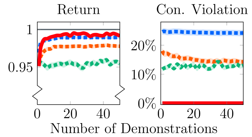
(a) Single environment.

(b) Transfer to new task.

(c) Transfer to new environment.

Figure 2: Experimental results in Gridworld environments. We consider three settings: (2(a)) no constraint transfer, (2(b)) transferring constraints to new goals in the same grid, and (2(c)) transferring constraints to a new Gridworld with the same structure but different transition dynamics. For each setting, we measure the normalized policy return (higher is better), and the constraint violation (lower is better). CoCoRL consistently returns safe solutions, outperforming the IRL-based methods that generally perform worse and are unsafe. The plots show mean and standard errors over 100 random seeds. A return greater than 1 indicates a solution that surpasses the best safe policy, implying a violation of safety constraints. The IRL methods use maximum entropy IRL. Appendix G provides results for maximum margin IRL, which show qualitatively similar findings.

6.1 IRL-based Constraint Learning Baselines

To the best of our knowledge, CoCoRL is the first algorithm that learns constraints from demonstrations with unknown rewards. Thus it is not immediately clear which baselines to compare it to. Nevertheless, we explore several IRL-based approaches that could serve as natural starting points for solving the constraint inference problem. Specifically, we consider the following three ways of applying IRL: (1) Average IRL infers a separate reward function $\hat{r}_{i}$ for each demonstration $\pi_{i}^{*}$ and averages the inferred rewards before combining them with an evaluation reward $r_{\text{eval}}+\sum_{i}\hat{r}_{i}/k$. (2) Shared Reward IRL parameterizes the inferred rewards as $\hat{r}_{i}+\hat{c}$, where $\hat{c}$ is shared among all demonstrations. The parameters for both the inferred rewards and the shared constraint penalty are learned simultaneously. (3) Known Reward IRL parameterizes the inferred reward as $r_{i}+\hat{c}$, where $r_{i}$ is known, and only a shared constraint penalty is learned. Note that Known Reward IRL has full access to the demonstrations’ rewards that the other methods do not need.

Each of these approaches can be implemented with any standard IRL algorithm. We primarily use Maximum Entropy IRL (Ziebart et al., 2008), but we also test Maximum Margin IRL (Ng et al., 2000) in tabular environments. We refer to Appendix E for more details on the IRL baselines.

6.2 Tabular Environments

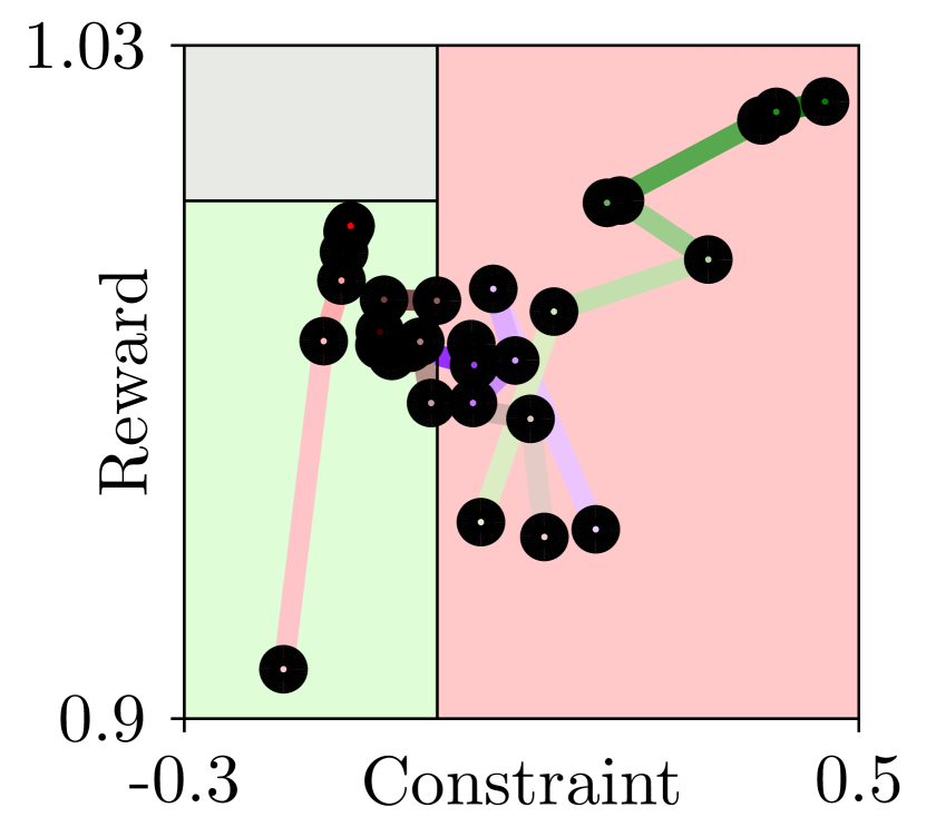
Figure 3: Illustration of safety and reward of CoCoRL, Average IRL, Shared Reward IRL, and Known Reward IRL in the Gridworld without constraint transfer. We show the $95$th percentile of the constraint and the corresponding reward. The lines are colored from light to dark to indicate increasing number of demonstrations. The green region is safe, the red region is unsafe, and the grey region would be safe but is unattainable. CoCoRL quickly reaches a safe and near-optimal solution. Known Reward IRL achieves a high reward but is unsafe. Shared Reward IRL and Average IRL are first unsafe and then safe but suboptimal.

We first consider tabular CMDPs which we can, conveniently, solve using linear programming (Altman, 1999). We construct a set of Gridworld environments that are structured as a 2D grid of cells. Each cell represents a state, and the agent can move left, right, up, down, or stay in the same cell. The environments have goal cells and limited cells. When the agent reaches a goal cell, it receives a reward; however, multiple constraints restrict how often the agent can visit the limited cells.

To introduce stochasticity, there is a fixed probability $p$ that the agent executes a random action instead of the intended one. The positions of the goal and limited cells are sampled uniformly at random. The reward and cost values are sampled uniformly from the interval $[0,1]$. The thresholds are also sampled uniformly, while we ensure feasibility via rejection sampling.

We perform three experiments to evaluate the transfer of learned constraints. First, we evaluate the learned constraints in the same environment and with the same reward distribution that they were learned from. Second, we change the reward distribution by sampling a new set of potential goals while keeping the constraints fixed. Third, we use a deterministic Gridworld ($p=0$) during training and a stochastic one ($p=0.2$) during evaluation.

Figure 2 presents the results of the experiments in $3\times 3$ Gridworlds. CoCoRL consistently returns safe policies and converges to the best safe solution as more demonstrations are provided. In contrast, none of the IRL-based methods learns safe policies. In the on-distribution evaluation shown in Figure 2(a), the IRL methods come closest to the desired safe policy but still cause many constraint violations.

Figure 3 provides an illustration of how the different methods trade off reward and safety. While CoCoRL always remains safe, the IRL baselines only achieve higher rewards by violating constraints.

6.3 Driving Environment

To explore a more practical and interesting environment, we consider highway-env, a 2D driving simulator (Leurent, 2018). We focus on a four-way intersection, as depicted in Figure 1. The agent drives towards the intersection and can turn left, right, or go straight. The environment is continuous, but it has a discrete high-level action space: the agent can accelerate, decelerate, and make turns at the intersection. There are three possible goals for the agent: turning left, turning right, or going straight. Additionally, the reward functions contain different driving preferences related to velocity and heading angle. Rewards and constraints are defined as a linear function of a state feature vector including goal indicators, vehicle position, velocity, heading, and indicators for unsafe events including crashing, leaving the street, and violating the speed limit.

For constrained policy optimization, we use a constrained cross-entropy method (CEM) to optimize a parametric driving controller (Wen and Topcu (2018); see Appendix D for details). We collect synthetic demonstrations that are optimized for different reward functions under a fixed set of constraints.

Similar to the previous experiments, we evaluate the learned constraints in three settings: (1) evaluation on the same task distribution and environment; (2) transfer to a new task; and (3) transfer to a modified environment. To transfer to a new task, we learn the constraints from trajectories only involving left and right turns at the intersection, but evaluate them on a reward function that rewards going straight (the situation illustrated in Figure 1). For the transfer to a modified environment, we infer constraints in an environment with very defensive drivers and evaluate them with very aggressive drivers. Additional details on the parameterization of other drivers can be found in Appendix F.

Empirically, we observe that the CEM occasionally fails to find a feasible policy when the safe set $\mathcal{S}$ is small. This is likely due to the CEM relying heavily on random exploration to discover an initial feasible solution. In situations where we cannot find a solution in $\mathcal{S}$, we return a “default” safe controller that remains safe but achieves a return of 0 because it just stands still before the intersection. Importantly, we empirically confirm that whenever we find a solution in $\mathcal{S}$, it is truly safe (i.e., in $\mathcal{F}$).

Figure 4 presents the results from the driving experiments. CoCoRL consistently guarantees safety, and with a larger enough number of demonstrations ($\sim 200$), CoCoRL returns high return policies. In contrast, Maximum Entropy IRL produces policies with decent performance in terms of return but they tend to be unsafe. Although the IRL solutions usually avoid crashes (which also result in low rewards), they disregard constraints that are in conflict with the reward function, such as the speed limits and keeping distance to other vehicles. IRL results in substantially more frequent constraint violations when trying to transfer the learned constraint penalty to a new reward. This is likely because the magnitude of the constraint penalty is no longer correct. CoCoRL does not suffer from this issue, and transferring the inferred constraints to a new reward still results in safe and well-performing policies.

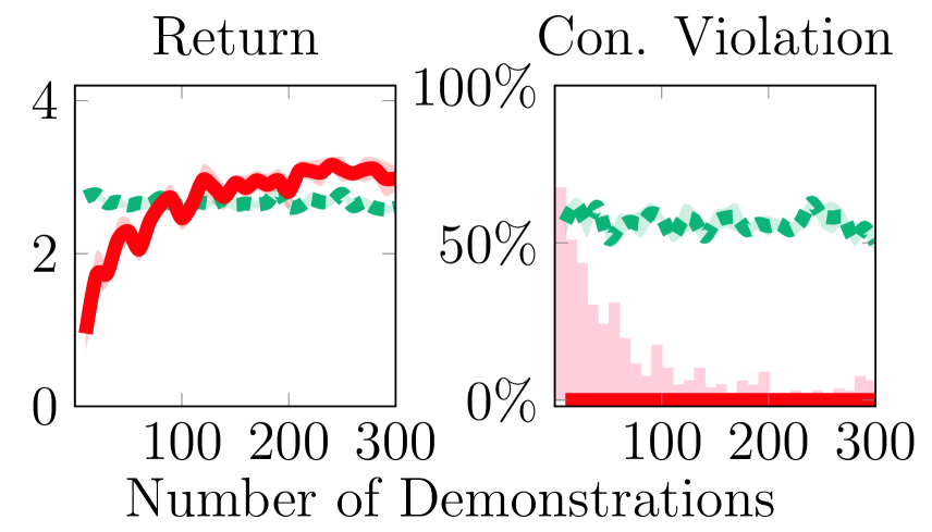
(a) Single environment.

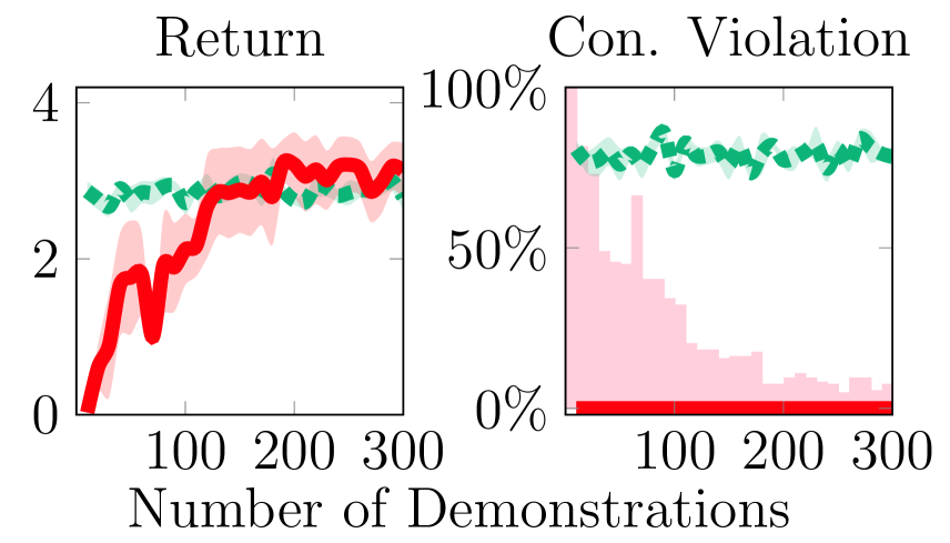
(b) Transfer to new task.

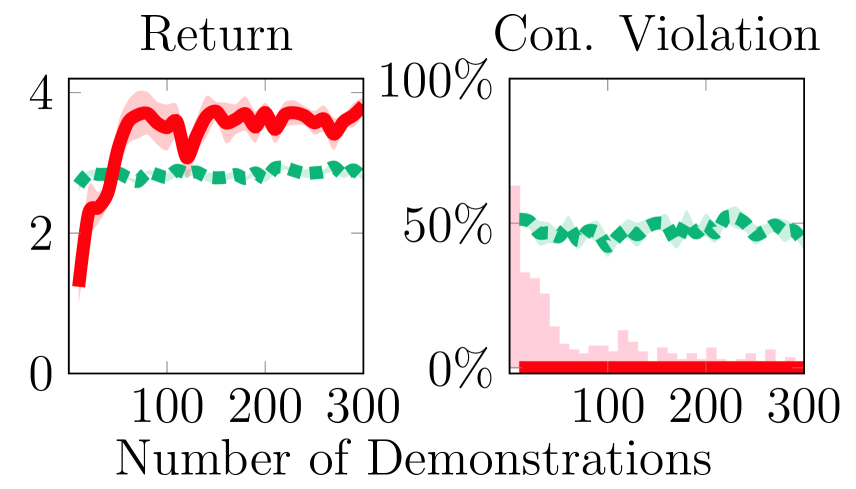
(c) Transfer to new environment.

Figure 4: Experimental results in the highway-env intersection environment, depicted in the form of return and constraint violation plots, similar to Figure 2. We compare the performance of CoCoRL () to that of maximum entropy IRL with known rewards (). All plots show mean and standard error over $5$ random seeds with a fixed set of evaluation rewards for each setting. In all settings, CoCoRL consistently returns safe policies, as indicated by the low constraint violation values. However, there are instances where CoCoRL falls back to providing a default safe solution when the policy optimizer fails to find a feasible solution within the safe set $\mathcal{S}$. The frequency of falling back to the default solution is shown by the bars in the constraint violation plots (). In contrast, the IRL method often yields unsafe solutions, indicated by the higher frequency of constraint violations.

7 Conclusion

We introduced CoCoRL, a novel algorithm for inferring shared constraints from demonstrations with unknown rewards. Theoretical and empirical results show that CoCoRL guarantees safety and achieves strong performance, even when transferring constraints to new tasks or environments.

Applications.

CoCoRL can use unlabeled demonstrations, which are often easier to obtain, particularly in domains such as robotics or autonomous driving. By learning safety constraints, CoCoRL offers a more sample-efficient and safer alternative to pure reward learning.

Limitations.

We assume that all demonstrations are safe, which may not always be practical. Learning from potentially unsafe demonstrations requires improved models of human demonstrations or additional (safety) labels. Our second assumption is access to a feature representation in non-tabular environments. As we scale CoCoRL to more complex applications, the ability to learn features that capture crucial safety aspects will become increasingly important.

Broader impact.

Constraint learning presents a promising approach to enhance the safety of reinforcement learning methods. While there are potential concerns about misuse or accidentally being overconfident in an agent’s safety, the same concerns apply more strongly to pure reward learning. Constraint has the potential to make reinforcement learning from human feedback more reliable and safer, thereby benefiting a wide range of applications.

Appendix

Appendix A Proofs of Theoretical Results

This section provides all proofs omitted in the main paper, as well as a few additional results related to estimating feature expectations (Section A.4).

A.1 Limitations of IRL in CMDPs

See 1

Proof.

This follows from the fact that there are CMDPs for which all feasible policies are stochastic. Every MDP, on the other hand, has a deterministic policy that is optimal (Puterman, 1990).

For example, consider a CMDP with a single state $S=\{s_{1}\}$ and two actions $A=\{a_{1},a_{2}\}$ with $P(s_{1}|s_{1},a_{1})=P(s_{1},|s_{1},a_{2})=1$. We have two cost functions $c_{1}(s_{1},a_{1})=1,c_{1}(s_{1},a_{2})=0$ and $c_{2}(s_{1},a_{1})=0,c_{2}(s_{1},a_{2})=1$, with thresholds $\xi_{1}=\xi_{2}=\frac{1}{2}$, and discount factor $\gamma=0$. To be feasible, a policy needs to have an occupancy measure $\mu_{\pi}$ such that $\sum_{s,a}\mu(s,a)c_{1}(s,a)\leq\xi_{1}$ and $\sum_{s,a}\mu_{\pi}(s,a)c_{2}(s,a)\leq\xi_{2}$.

In our case with a single state and $\gamma=0$, this simply means that a feasible policy $\pi$ needs to satisfy $\pi(a_{1}|s_{1})\leq\frac{1}{2}$ and $\pi(a_{2}|s_{1})\leq\frac{1}{2}$. But this implies that only a uniformly random policy is feasible.

Any IRL algorithm infers a reward function that matches the occupancy measure of the expert policy (Abbeel and Ng, 2004). Consequently, the inferred reward $r_{\text{IRL}}$ needs to give both actions the same reward, because otherwise $\pi^{*}$ would not be optimal for the MDP with $r_{\text{IRL}}$. However, that MDP also has a deterministic optimal policy (like any MDP), which is not feasible in the original CMDP. ∎

See 2

Proof.

As in the proof of Proposition 1, we consider a single-state CMDP with $S=\{s_{1}\}$ and $A=\{a_{1},a_{2}\}$, where $a_{1}$. We have $c_{1}(s_{1},a_{1})=1,c_{1}(s_{1},a_{2})=0$ and $c_{2}(s_{1},a_{1})=0,c_{2}(s_{1},a_{2})=1$, $\xi_{1}=\xi_{2}=\frac{1}{2}$, and $\gamma=0$. Again, the only feasible policy uniformly randomizes between $a_{1}$ and $a_{2}$.

Let $r_{1}(a_{1})=1$, $r_{1}(a_{2})=1$, $r_{2}(a_{1})=0$, $r_{2}(a_{2})=1$, i.e., the first reward function gives equal reward to both actions and the second reward function gives inequal rewards (for simplicity we write $r(a)=r(s,a)$). To make the uniformly random policy optimal in $\mathcal{M}\cup\{r_{1}+\hat{c}\}$ and $\mathcal{M}\cup\{r_{2}+\hat{c}\}$, both inferred reward functions $r_{1}+\hat{c}$ and $r_{2}+\hat{c}$ need to give both actions equal rewards. However this is clearly impossible. If $r_{1}(a_{2})+\hat{c}(a_{2})-(r_{1}(a_{1})+\hat{c}(a_{1}))=0$, then

$$r_{2}(a_{2})+\hat{c}(a_{2})-(r_{2}(a_{1})+\hat{c}(a_{1}))$$

$$= r_{2}(a_{2})-r_{1}(a_{2})+r_{1}(a_{2})+\hat{c}(a_{2})-(r_{2}(a_{1})-r_{1}(a_{1})+r_{1}(a_{1})+\hat{c}(a_{1}))$$

$$= \underbrace{r_{2}(a_{2})-r_{1}(a_{2})}_{=0}-\underbrace{(r_{2}(a_{1})-r_{1}(a_{1}))}_{=-1}+\underbrace{r_{1}(a_{2})+\hat{c}(a_{2})-(r_{1}(a_{1})+\hat{c}(a_{1}))}_{=0}=1\neq 0.$$

∎

A.2 Safety Guarantees

See 2

Proof.

The convex hull of a set of points is a convex polyhedron, i.e., it is the solution of a set of linear equations (see, e.g., Theorem 2.9 in Pulleyblank, 1983).

Hence, $\mathcal{S}$ is a convex polyhedron in the feature space defined by $\mathbf{f}$, i.e., we can find $A\in\mathbb{R}^{p\times d},\mathbf{b}\in\mathbb{R}^{p}$ such that

$$\mathcal{S}=\{x\in\mathbb{R}^{d}|Ax\leq\mathbf{b}\}.$$

To construct $A$ and $\mathbf{b}$, we need to find the facets of $\mathcal{S}$, the convex hull of a set of points $\mathcal{D}$. This is a standard problem in polyhedral combinatorics (e.g., see Pulleyblank, 1983).

We can now define $p$ linear constraint functions $\hat{c}_{j}(s,a)=A_{j}\mathbf{f}(s,a)$ and thresholds $\hat{\xi}_{j}=b_{j}$, where $A_{j}$ is the $j$-th row of $A$ and $b_{j}$ is the $j$-th component of $\mathbf{b}$ (for $j=1,\dots,p$. Then, solving the CMDP $(S,A,P,\mu_{0},\gamma,r_{\text{eval}},\{\hat{c}_{j}\}_{j=1}^{p}\{\hat{\xi}_{j}\}_{j=1}^{p})$ corresponds to solving

$$\pi^{*}\in\mathop{\mathrm{missing}}{argmax}_{\hat{J}_{1}(\pi)\leq\hat{\xi}_{1},\dots,\hat{J}_{p}(\pi)\leq\hat{\xi}_{p}}G_{r_{\text{eval}}}(\pi).$$

For these linear cost functions, we can rewrite the constraints using the discounted feature expectations as $J_{i}(\pi)=A_{i}\mathbf{f}(\pi)$. Hence, $\pi$ satisfying the constraints $\hat{J}_{1}(\pi)\leq\hat{\xi}_{1},\dots,\hat{J}_{p}(\pi)\leq\hat{\xi}_{p}$ is equivalent to $\pi\in\mathcal{S}$. ∎

See 1

Proof.

Using Theorem 2, we can construct a set of cost functions $\{c_{j}\}_{j=1}^{n}$ and thresholds $\{\xi_{j}\}_{j=1}^{n}$ for which $\pi\in\mathcal{S}$ is equivalent to $J_{1}(\pi)\leq\xi_{1},\dots,J_{n}(\pi)\leq\xi_{n}$. Hence, in a CMDP with these cost functions and thresholds, any policy $\pi\notin\mathcal{S}$ is not feasible. Because $\pi_{1}^{*},\dots,\pi_{k}^{*}\in\mathcal{S}$ by construction, each $\pi^{*}_{i}$ is optimal in the CMDP $(S,A,P,\mu_{0},\gamma,r_{i},\{c_{j}\}_{j=1}^{n},\{\xi_{j}\}_{j=1}^{n})$. ∎

A.3 Optimality Guarantees

Lemma 2.

For any policy $\pi$, if $r:S\times A\to[0,1]$ and $\mathbf{f}:S\times A\to[0,1]^{d}$, we can bound

$$\forall i:~{}\mathbf{f}(\pi)_{i} \leq\frac{1}{1-\gamma} \|\mathbf{f}(\pi)\|_{2}\leq\frac{\sqrt{d}}{1-\gamma}$$

$$G_{r}(\pi) \leq\frac{d}{1-\gamma} \mathcal{R}(\pi,\mathcal{S})\leq\frac{2d}{1-\gamma}$$

Proof.

First, we have for any component of the feature expectations

$$\mathbf{f}_{i}(\pi)=\mathbb{E}[\sum_{t=0}^{\infty}\gamma^{t}\mathbf{f}(s_{t},a_{t})]\leq\sum_{t=0}^{\infty}\gamma^{t}=\frac{1}{1-\gamma},$$

using the limit of the geometric series. This immediately gives

$$\|\mathbf{f}(\pi)\|_{2}=\sqrt{\sum_{i=1}^{d}\mathbf{f}(\pi)_{i}^{2}}\leq\frac{\sqrt{d}}{1-\gamma}.$$

Similarly bounded rewards $r(s,a)\leq 1$ imply $\|\theta\|_{2}\leq\sqrt{d}$. Together, we can bound the returns using the Cauchy-Schwartz inequality

$$G_{r}(\pi)=\|\theta^{T}\mathbf{f}(\pi)\|_{2}\leq\|\theta\|_{2}\cdot\|\mathbf{f}(\pi)\|_{2}\leq\frac{d}{1-\gamma}.$$

Further, for any two policies $\pi_{1},\pi_{2}$, we have $G_{r}(\pi_{1})-G_{r}(\pi_{2})\leq\frac{2d}{1-\gamma}$, which implies the same for the regret $\mathcal{R}(r,\mathcal{S})\leq\frac{2d}{1-\gamma}$. ∎

See 3

Proof.

The true safe set and the estimated safe set are convex polyhedra, and we have a finite hypothesis class: all polyhedra with vertices are a subset of the true safe set’s vertices.

Consider the distribution over optimal policies $P(\mathbf{f}(\pi^{*}))$ induced by $P(r)$. The support of $P(\mathbf{f}(\pi^{*}))$ are the vertices of the true safe set.

We can distinguish two cases. Case 1: we have seen a vertex corresponding to an optimal policy for $r$ in the first $k$ demonstrations; and, Case 2: we have not. In Case 1, we incur $0$ regret, and only in Case 2 we can incur regret greater than $0$.

So, we can bound the probability of incurring regret by the probability of Case 2:

$$P(\mathcal{R}(r,\mathcal{S}_{k})>0)\leq\sum_{\text{vertex }\mathbf{v}}(1-P(\mathbf{v}))^{k}P(\mathbf{v}).$$

To ensure $P(\mathcal{R}(r,\mathcal{S}_{k})>0)\leq\delta$, it is sufficient to ensure that each term of the sum satisfies $(1-P(\mathbf{v}))^{k}P(\mathbf{v})\leq\delta/N_{v}$ where $N_{v}$ is the number of vertices. For terms with $P(\mathbf{v})\leq\delta/N_{v}$ this is true for all $k$. For the remaining terms with $P(\mathbf{v})>\delta/N_{v}$, we can write

$$(1-P(\mathbf{v}))^{k}P(\mathbf{v})\leq(1-\delta/N_{v})^{k}.$$

So, it is sufficient to ensure $(1-\delta/N_{v})^{k}\leq\delta/N_{v}$, which is satisfied once

$$k>\frac{\log(\delta/N_{v})}{\log(1-\delta/N_{v})}.$$

By replacing $N_{v}$ with a suitable upper bound on the number of vertices, we arrive at the first result.

By Lemma 2, the maximum regret is upper-bounded by $\frac{2d}{1-\gamma}$, and, we can decompose the regret as

$$\mathbb{E}_{r}[\mathcal{R}(r,\mathcal{S}_{k})]\leq\frac{2d}{1-\gamma}\sum_{\text{vertex }\mathbf{v}}(1-P(\mathbf{v}))^{k}P(\mathbf{v})\leq\frac{2d}{1-\gamma}\sum_{\mathbf{v}:P(\mathbf{v})>0}(1-P(\mathbf{v}))^{k}.$$

Because $P(\mathbf{v})$ is a fixed distribution induced by $P(r)$, the r.h.s. converges to $0$ as $k\to\infty$. ∎

Lemma 3.

Under Assumption 2, we have for any reward function $r$ and any feasible policy $\pi\in\mathcal{F}$

$$P(\pi)\geq\exp(-\beta d/(1-\gamma)).$$

Proof.

We have $\beta>0$ and $G_{r}(\pi)\geq 0$, which implies $\exp(\beta G_{r}(\pi))\geq 1$, and

$$P(\pi|r)=\frac{\exp(\beta G_{r}(\pi)}{Z(\theta)}\geq\frac{1}{Z(\theta)}.$$

By Lemma 2, we have $G_{r}(\pi)\leq d/(1-\gamma)$. Therefore,

$$Z(\theta)=\int_{\pi\in\mathcal{F}}\exp(\beta\theta^{T}\mathbf{f}(\pi))\mathrm{d}\pi\leq\exp(\beta d/(1-\gamma)),$$

and

$$P(\pi|r)\geq\exp(-\beta d^{2}/(1-\gamma)).$$

∎

See 4

Proof.

We can upper-bound the probability of having non-zero regret similar to the noise free case by

$$P(\mathcal{R}(r,\mathcal{S}_{k})>0)\leq\sum_{\text{vertex }\mathbf{v}}(1-P(\mathbf{v}))^{k}P(\mathbf{v}).$$

Under Assumption 2, we can use Lemma 3, to obtain

$$P(\mathbf{v})\geq\exp(-\beta d/(1-\gamma))\coloneqq\Delta.$$

Importantly, $0<\Delta<1$ is a constant, and we have

$$P(\mathcal{R}(r,\mathcal{S}_{k})>0)\leq\sum_{\text{vertex }\mathbf{v}}(1-\Delta)^{k}.$$

To ensure $P(\mathcal{R}(r,\mathcal{S}_{k})>0)\leq\delta$, it is sufficient to ensure $(1-\Delta)^{k}\leq\delta/N_{v}$, where $N_{v}$ is the number of vertices of the true safe set. This is true once

$$k\geq\frac{\log(\delta/N_{v})}{\log(1-\exp(-\beta d/(1-\gamma)))},$$

where we can again replace $N_{v}$ by a suitable upper bound.

Bounding the maximum regret via Lemma 2, we get

$$\mathbb{E}_{r}[\mathcal{R}(r,\mathcal{S}_{k})]\leq\frac{2d}{1-\gamma}\sum_{\text{vertex }\mathbf{v}}(1-\Delta)^{k},$$

which converges to $0$ as $k\to\infty$. ∎

A.4 Estimating Feature Expectations

Lemma 4.

Let $\pi$ be a policy with true feature expectation $\mathbf{f}(\pi)$. We estimate the feature expectation using $n_{\text{traj}}$ trajectories $\tau_{i}$ collected by rolling out $\pi$ in the environment: $\hat{\mathbf{f}}(\pi)=\frac{1}{n_{\text{traj}}}\sum_{i=1}^{n_{\text{traj}}}\mathbf{f}(\tau_{i})$. This estimate is unbiased, i.e., $\mathbb{E}[\hat{\mathbf{f}}(\pi)]=\mathbf{f}(\pi)$. Further let $\phi\in\mathbb{R}^{d}$ be a vector, such that, $0\leq\phi^{T}\mathbf{f}(s,a)\leq 1$ for any state $s$ and action $a$. Then, we have for any $\epsilon>0$

$$P(\phi^{T}\hat{\mathbf{f}}(\pi)-\phi^{T}\mathbf{f}(\pi)\geq\epsilon) \leq\exp(-2\epsilon^{2}n_{\text{traj}}(1-\gamma)/d),$$

$$P(\phi^{T}\mathbf{f}(\pi)-\phi^{T}\hat{\mathbf{f}}(\pi)\geq\epsilon) \leq\exp(-2\epsilon^{2}n_{\text{traj}}(1-\gamma)/d).$$

Proof.

Because the expectation is linear, the estimate is unbiased, and, $\mathbb{E}[\phi^{T}\hat{\mathbf{f}}(\pi)]=\phi^{T}\mathbf{f}(\pi)$.

For any trajectory $\tau$ and any $1\leq i\leq d$, we have $0\leq\mathbf{f}_{i}(\tau)\leq 1/(1-\gamma)$, and, consequently, $0\leq\phi^{T}\mathbf{f}(\tau)\leq d/(1-\gamma)$, analogously to Lemma 2). Thus, $\phi^{T}\hat{\mathbf{f}}(\pi)$ satisfies the bounded difference property. In particular, by changing one of the observed trajectories, the value of $\phi^{T}\hat{\mathbf{f}}(\pi)$ can change at most by $d/(n_{\text{traj}}(1-\gamma))$. Hence, by McDiarmid’s inequality, we have for any $\epsilon>0$

$$P(\theta^{T}\hat{\mathbf{f}}(\pi)-\mathbb{E}[\theta^{T}\hat{\mathbf{f}}(\pi)]\geq\epsilon)\leq\exp\left(-\frac{2\epsilon^{2}}{d/(n_{\text{traj}}(1-\gamma))}\right),$$

and

$$P(\theta^{T}\hat{\mathbf{f}}(\pi)-\theta^{T}\mathbf{f}(\pi)\geq\epsilon)\leq\exp\left(-\frac{2\epsilon^{2}n_{\text{traj}}(1-\gamma)}{d}\right).$$

We can bound $P(\phi^{T}\mathbf{f}(\pi)-\phi^{T}\hat{\mathbf{f}}(\pi)\geq\epsilon)$ analogously. ∎

See 5

Proof.

Let us define the “good” event that for policy $\pi_{i}^{*}$ we accurately estimate the value of the cost function $c_{j}$ and denote it by $\mathcal{E}_{ij}=\{\phi_{j}^{T}\hat{\mathbf{f}}(\pi_{i}^{*})-\phi_{j}^{T}\mathbf{f}(\pi_{i}^{*})\leq\epsilon\}$, where $\phi_{j}$ parameterizes $c_{j}$. Conditioned on $\mathcal{E}_{ij}$ for all $i$ and $j$, we have

$$P(\max_{j}(J_{j}(\pi)-\xi_{j}) >\epsilon|\pi\in\hat{\mathcal{S}},\{\mathcal{E}_{ij}\})\leq\sum_{j}P((J_{j}(\pi)-\xi_{j})>\epsilon|\pi\in\hat{\mathcal{S}},\{\mathcal{E}_{ij}\})$$

$$=\sum_{j}P(\phi_{j}^{T}\sum_{l}\lambda_{l}\hat{\mathbf{f}}(\pi_{l}^{*})>\xi_{j}+\epsilon|\{\mathcal{E}_{ij}\})=0.$$

Hence, we can bound the probability of having an unsafe policy by the probability of the “bad” event, which we can bound by Lemma 4 to obtain

$$P(\max_{j}(J_{j}(\pi)-\xi_{j})>\epsilon|\pi\in\hat{\mathcal{S}})\leq\sum_{ij}P(\text{not }\mathcal{E}_{ij})\leq n\cdot k\cdot\exp(-2\epsilon^{2}n_{\text{traj}}(1-\gamma)/d).$$

So, to ensure $P(\max_{j}(J_{j}(\pi)-\xi_{j})>\epsilon|\pi\in\hat{\mathcal{S}}\})\leq\delta$, it is sufficient to ensure

$$\exp(-2\epsilon^{2}n_{\text{traj}}(1-\gamma)/d)\leq\frac{\delta}{nk},$$

which is true if we collect at least

$$n_{\text{traj}}>\frac{d\log(nk/\delta)}{2\epsilon^{2}(1-\gamma)}$$

trajectories for each policy. ∎

Theorem 6 (Convergence, noise-free, estimated feature expectations).

Under Assumption 1, if we estimate the feature expectations of at least $k>\log(\delta/(2f_{v}(d,n)))/\log(1-\delta/(2f_{v}(d,n)))$ expert policies using at least $n_{\text{traj}}>d\log(2f_{v}(d,n)/\delta)/(2\epsilon^{2}(1-\gamma))$ samples each, we have $P(\mathcal{R}(r,\mathcal{S}_{k})>\epsilon)\leq\delta$, where $f_{v}(d,n)$ is an upper bound on the number of vertices of the true safe set. In particular, we have $\lim_{\min(k,n_{\text{traj}})\to\infty}\mathbb{E}_{r}\left[\mathcal{R}(r,\mathcal{S}_{k})\right]=0$.

Proof.

To reason about the possibility of a large estimation error for the feature expectations, we use Lemma 4 to lower bound the probability of the good event $\mathcal{E}_{\mathbf{v}}=\{\theta^{T}\mathbf{v}-\theta^{T}\hat{\mathbf{f}}(\pi_{i}^{*})\leq\epsilon\}$, for each vertex $\mathbf{v}$ of the true safe set.

For an evaluation reward $r_{\text{eval}}$, we can incur regret in one of three cases:
Case 1: we have not seen a vertex corresponding to an optimal policy for $r_{\text{eval}}$.
Case 2: we have seen an optimal vertex but our estimation of that vertex is bad.
Case 3: we have seen an optimal vertex and our estimation of that vertex is good.

We show that the probability of Case 1 shrinks as we increase $k$, the probability of Case 2 shrinks as we increase $n_{\text{traj}}$, and the regret that we can incur in Case 3 is small.

Case 1: This case is independent of the estimated feature expectations. Similar to Theorem 3, we can bound its probability for each vertex $\mathbf{v}$ by $(1-P(\mathbf{v}))^{k}P(\mathbf{v})$.

Case 2: In case of the bad event, i.e., the complement of $\mathcal{E}_{\mathbf{v}}$, we can upper-bound the probability of incurring high regret using Lemma 4, to obtain

$$P(\theta^{T}\mathbf{v}-\theta^{T}\hat{\mathbf{f}}(\pi_{i}^{*})>\epsilon|\text{not }\mathcal{E}_{\mathbf{v}})P(\text{not }\mathcal{E}_{\mathbf{v}})\leq P(\text{not }\mathcal{E}_{\mathbf{v}})\leq\exp(-2\epsilon^{2}n_{\text{traj}}(1-\gamma)/d).$$

Case 3: Under the good event $\mathcal{E}_{\mathbf{v}}$, we automatically have regret less than $\epsilon$, i.e.,

$$P(\theta^{T}\mathbf{v}-\theta^{T}\hat{\mathbf{f}}(\pi_{i}^{*})>\epsilon|\mathcal{E}_{\mathbf{v}})P(\mathcal{E}_{\mathbf{v}})=0.$$

Using these three cases, we can now bound the probability of having regret greater than $\epsilon$ as

$$P(\mathcal{R}(r,\mathcal{S}_{k})>\epsilon)\leq\sum_{\text{vertex }\mathbf{v}}\Bigl{(}\underbrace{(1-P(\mathbf{v}))^{k}P(\mathbf{v})}_{\textbf{Case 1}}+\underbrace{\exp(-2\epsilon^{2}n_{\text{traj}}(1-\gamma)/d)}_{\textbf{Case 2}}+\underbrace{0}_{\textbf{Case 3}}\Bigr{)}.$$

To ensure that $P(\mathcal{R}(r,\mathcal{S}_{k})>\epsilon)\leq\delta$, it is sufficient to ensure each term of the sum is less than $\delta/N_{v}$ where $N_{v}$ is the number of vertices. We have two terms inside the sum, so it is sufficient to ensure either term is less than $\delta/(2N_{v})$.

Case 1: We argue analogously to Theorem 3. For terms with $P(\mathbf{v})\leq\delta/(2N_{v})$ it is true for all $k$. For the remaining terms with $P(\mathbf{v})>\delta/(2N_{v})$, we can use

$$(1-P(\mathbf{v}))^{k}P(\mathbf{v})\leq(1-\delta/(2N_{v}))^{k}$$

so it is sufficient to ensure

$$(1-\delta/(2N_{v}))^{k}\leq\delta/(2N_{v})$$

which is satisfied once

$$k>\frac{\log(\delta/(2N_{v}))}{\log(1-\delta/(2N_{v}))}.$$

This is our first condition.

Case 2: To ensure $\exp(-2\epsilon^{2}n_{\text{traj}}(1-\gamma)/d)\leq\delta/(2N_{v})$, we need

$$n_{\text{traj}}>\frac{d\log(2N_{v}/\delta)}{2\epsilon^{2}(1-\gamma)}.$$

This is our second condition.

If both conditions hold simultaneously, we have $P(\mathcal{R}(r,\mathcal{S}_{k})>\epsilon)\leq\delta$.

To analyse the regret, let us consider how $\epsilon$ shrinks as a function of $n_{\text{traj}}$. The analysis above holds for any $\epsilon$. So, for a given $k$ and $n_{\text{traj}}$, we need to chose

$$\epsilon^{2}\geq\frac{d\log(2nkN_{v}/\delta)}{2n_{\text{traj}}(1-\gamma)}$$

to guarantee $P(\mathcal{R}(r,\mathcal{S}_{k})>\epsilon)\leq\delta$. Hence, the smallest $\epsilon$ we can choose is

$$\epsilon_{\min}=\sqrt{\frac{d\log(2nkN_{v}/\delta)}{2n_{\text{traj}}(1-\gamma)}}.$$

Using Lemma 2 to upper-bound the maximum regret by $\frac{2d^{2}}{1-\gamma}$, we can upper-bound the expected regret by

$$\mathbb{E}_{r}[\mathcal{R}(r,\mathcal{S}_{k})]\leq\frac{2d^{2}}{1-\gamma}P(\mathcal{R}(r,\mathcal{S}_{k})>\epsilon_{\min})+\epsilon_{\min}P(\mathcal{R}(r,\mathcal{S}_{k})\leq\epsilon_{\min})$$

$$\leq\frac{2d}{1-\gamma}\sum_{\mathbf{v}:P(\mathbf{v})>0}(1-P(\mathbf{v}))^{k}+\frac{2dN_{v}}{1-\gamma}\exp(-2\epsilon_{\min}^{2}(1-\gamma)/d)\frac{k}{\exp(n_{\text{traj}})}+\sqrt{\frac{d\log(2nkN_{v}/\delta)}{2n_{\text{traj}}(1-\gamma)}}.$$

For each term individually, we can see that it converges to $0$ as $\min(k,n_{\text{traj}})\to\infty$:

$$\lim_{\min(k,n_{\text{traj}})\to\infty}\sum_{\mathbf{v}:P(\mathbf{v})>0}(1-P(\mathbf{v}))^{k}=\lim_{k\to\infty}\sum_{\mathbf{v}:P(\mathbf{v})>0}(1-P(\mathbf{v}))^{k}=0,$$

$$\lim_{\min(k,n_{\text{traj}})\to\infty}\underbrace{\exp(-2\epsilon_{\min}^{2}(1-\gamma)/d)}_{\leq 1}\frac{k}{\exp(n_{\text{traj}})}\leq\lim_{\min(k,n_{\text{traj}})\to\infty}\frac{k}{\exp(n_{\text{traj}})}=0,$$

$$\lim_{\min(k,n_{\text{traj}})\to\infty}\sqrt{\frac{d\log(2nkN_{v}/\delta)}{2n_{\text{traj}}(1-\gamma)}}=0.$$

Hence, $\lim_{\min(k,n_{\text{traj}})\to\infty}\mathbb{E}_{r}[\mathcal{R}(r,\mathcal{S}_{k})]=0$. ∎

Theorem 7 (Convergence under Boltzmann noise, estimated feature expectations).

Under Assumption 2, if we estimate the feature expectations of at least $k>\log(\delta/(2f_{v}(d,n)))/(\log(1-\exp(-\beta d/(1-\gamma))))$ expert policies using at least $n_{\text{traj}}>d\log(2f_{v}(d,n)/\delta)/(2\epsilon^{2}(1-\gamma))$ samples each, we have $P(\mathcal{R}(r,\mathcal{S}_{k})>\epsilon)\leq\delta$, where $f_{v}(d,n)$ is an upper bound on the number of vertices of the true safe set. In particular, we have $\lim_{\min(k,n_{\text{traj}})\to\infty}\mathbb{E}_{r}\left[\mathcal{R}(r,\mathcal{S}_{k})\right]=0$.

Proof.

We can decompose the probability of incurring regret greater than $\epsilon$ into the same three cases discussed in the proof of Theorem 6 to get the upper-bound

$$P(\mathcal{R}(r,\mathcal{S}_{k})>\epsilon)\leq\sum_{\text{vertex }\mathbf{v}}\Bigl{(}\underbrace{(1-P(\mathbf{v}))^{k}P(\mathbf{v})}_{\textbf{Case 1}}+\underbrace{\exp(-2\epsilon^{2}n_{\text{traj}}(1-\gamma)/d)}_{\textbf{Case 2}}+\underbrace{0}_{\textbf{Case 3}}.\Bigr{)}$$

Under Assumption 2, we can use Lemma 3, to get

$$P(\mathbf{v})\geq\exp(-\beta d/(1-\gamma))\coloneqq\Delta.$$

Combining both bounds, we get

$$P(\mathcal{R}(r,\mathcal{S}_{k})>\epsilon)\leq\sum_{\text{vertex }\mathbf{v}}\Bigl{(}(1-\Delta)^{k}+\exp(-2\epsilon^{2}n_{\text{traj}}(1-\gamma)/d)\Bigr{)}.$$

To ensure $P(\mathcal{R}(r,\mathcal{S}_{k})>\epsilon)\leq\delta$ it is sufficient to ensure both $(1-\Delta)^{k}\leq\delta/(2N_{v})$ and $\exp(-2\epsilon^{2}n_{\text{traj}}(1-\gamma)/d\leq\delta/(2N_{v})$ where $N_{v}$ is the number of vertices of the true safe set. This is true once

$$k>\frac{\log(\delta/(2N_{v}))}{\log(1-\Delta)}=\frac{\log(\delta/(2N_{v}))}{\log(1-\exp(-\beta d/(1-\gamma)))},$$

and

$$n_{\text{traj}}>\frac{d\log(2N_{v}/\delta)}{2\epsilon^{2}(1-\gamma)},$$

where can again replace $N_{v}$ by a suitable upper bound.

For the regret, we get asymptotic optimality with the same argument from the proof of Theorem 6, replacing $P(\mathbf{v})$ with the constant $\Delta$. ∎

Appendix B Constructing a Conservative Safe Set from Estimated Feature Expectations

Theorem 5 shows that we can guarantee $\epsilon$-safety even when estimating the feature expectations of the demonstrations. However, sometimes we need to ensure exact safety. In this section, we discuss how we can use confidence intervals around estimated feature expectations to construct a conservative safe set, i.e., a set $\hat{\mathcal{S}}\subset\mathcal{S}$ that still guarantees exact safety with high probability (w.h.p.).

Suppose we have $k$ confidence sets $\mathcal{C}_{i}\subseteq\mathbb{R}^{d}$, such that we know $\mathbf{f}(\pi_{i}^{*})\in\mathcal{C}_{i}$ (w.h.p.). Now we want to construct a conservative convex hull, i.e., a set of points in which any point certainly in the convex hull of $\mathbf{f}(\pi_{1}^{*}),\dots,\mathbf{f}(\pi_{k}^{*})$. In other words, we want to construct the intersection of all possible convex hulls with points from $\mathcal{C}_{1},\dots,\mathcal{C}_{k}$:

$$\hat{S}=\bigcap\limits_{x_{1},\dots,x_{k}\in\mathcal{C}_{1}\times\dots\times\mathcal{C}_{k}}\mathtt{conv}(x_{1},\dots,x_{k}).$$

This set is sometimes called the guaranteed hull (Sember, 2011), or the interior convex hull (Edalat et al., 2005). Efficient algorithms are known to construct guaranteed hulls in $2$ or $3$ dimensions if $\mathcal{C}$ has a simple shape, such as a cube or a disk (e.g., see Sember, 2011). However, we need to construct a guaranteed hull in $d$ dimensions.

Edalat et al. (2001) propose to reduce the problem of constructing guaranteed hull when $\mathcal{C}_{i}$ are (hyper-)rectangles to computing the intersection of convex hulls constructed from combinations of the corners of the rectangle. In $d\leq 3$ dimensions, this is possible with $\mathcal{O}(k\log k)$ complexity, but in higher dimensions is requires $\mathcal{O}(k^{\lfloor d/2\rfloor})$. If we use a concentration inequality for each coordinate independently, e.g., by using Lemma 4 with unit basis vectors, then the $\mathcal{C}_{i}$’s are rectangles, and we can use this approach. However, because we have to construct many convex hulls, it can get expensive as $k$ and $d$ grow.

Figure 5 illustrates the guaranteed hull growing as the confidence regions shrink. The guaranteed hull is a conservative estimate and can be empty if the $\mathcal{C}_{i}$’s are too large. Hence, $\hat{\mathcal{S}}$ might be too conservative sometimes, especially if we cannot observe multiple trajectories from the same policy. In such cases, we need additional assumptions about the environment (e.g., it is deterministic) or the demonstrations (e.g., every trajectory is safe) to guarantee safety in practice. Still, using a guaranteed hull as a conservative safe set is a promising alternative to relying on point estimates of the feature expectations.

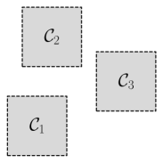
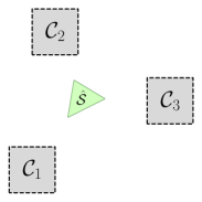
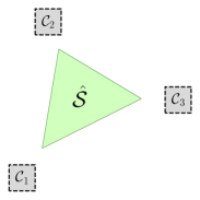
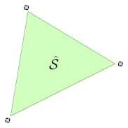
Figure 5: Illustration of the guaranteed hull in 2D. The gray areas depict confidence sets $\mathcal{C}_{1},\mathcal{C}_{2},\mathcal{C}_{3}$, and the green area is the conservative safe set $\hat{\mathcal{S}}$ constructed using the guaranteed hull. For large confidence sets, the guaranteed hull can be empty (left); for small confidence sets, it approaches the safe set constructed using the exact feature expectations (right).

Appendix C Excluding Guaranteed Unsafe Policies

In the main paper, we showed that $\mathcal{S}$ guarantees safety and that we cannot safely expand that set. In this section, we discuss how we can distinguish policies that we know are unsafe from policies we are still uncertain about. First, we note that, in general, this is impossible. For example, if the expert reward functions are all-zero $r_{i}(s,a)=0$, any policy outside $\mathcal{S}$ might still be in $\mathcal{F}$. However, if we exclude such degenerate cases, we can expect expert policies to lie on the boundary of $\mathcal{F}$, which gives us some additional information.

Hence, in this section, we assume optimal demonstrations (Assumption 1), and we make an additional (mild) assumption to exclude degenerate demonstrations.

Assumption 3 (Non-degenerate demonstrations).

For each expert reward function $r_{i}$ there are at least two expert policies $\pi_{j}^{*},\pi_{l}^{*}$ that have different returns under $r_{i}$, i.e., $G_{r_{i}}(\pi_{j}^{*})\neq G_{r_{i}}(\pi_{l}^{*})$.

Now, we construct the “unsafe” set $\mathcal{U}=\cup_{i=1}^{k}\mathcal{U}_{i}$ with

$$\mathcal{U}_{i}=\{x\in\mathbb{R}^{d}|\exists\alpha_{1},\dots,\alpha_{i-1},\alpha_{i+1},\dots\alpha_{k}>0\text{ s.t. }x-\mathbf{f}(\pi_{i}^{*})=\sum_{j\neq i}\alpha_{j}(\mathbf{f}(\pi_{i}^{*})-\mathbf{f}(\pi_{j}^{*}))\}.$$

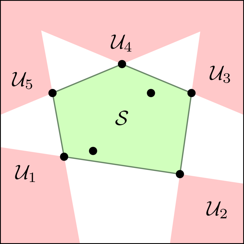
Figure 6: Illustration of safe set and “unsafe” set in 2D.

For simplicity, we will sometimes write $\pi\in\mathcal{U}$ instead of $\mathbf{f}(\pi)\in\mathcal{U}$. At each vertex $i$ of the safe set, $\mathcal{U}_{i}$ is a convex cone of points incompatible with observing $\pi_{i}^{*}$. In particular, any point in $\mathcal{U}_{i}$ is strictly better than $\pi_{i}^{*}$, i.e., for any reward function for which $\pi_{i}^{*}$ is optimal, a point in $\mathcal{U}_{i}$ would be better than $\pi_{i}^{*}$. Figure 6 illustrates this construction. We can show that any policy in $\mathcal{U}$ is guaranteed not to be in $\mathcal{F}$, and that $\mathcal{U}$ is the largest possible set with this property.

Theorem 8.

Under Assumption 1 and Assumption 3, $\mathcal{U}\cap\mathcal{F}=\emptyset$. In particular, any $\pi\in\mathcal{U}$ is not in $\mathcal{F}$.

Proof.

Assume there is a policy $\pi\in\mathcal{U}\cap\mathcal{F}$. Then, by construction, there is an $1\leq i\leq k$ such that $\pi\in\mathcal{U}_{i}$, i.e., there are $\alpha_{1},\dots,\alpha_{i-1},\alpha_{i+1},\dots,\alpha_{k}>0$, such that

$$\mathbf{f}(\pi)-\mathbf{f}(\pi_{i}^{*})=\sum_{j\neq i}\alpha_{j}(\mathbf{f}(\pi_{i}^{*})-\mathbf{f}(\pi_{j}^{*})).$$

We know that $\pi_{i}^{*}$ is optimal for a reward function $r_{i}(s,a)=\theta_{i}^{T}\mathbf{f}(s,a)$ parameterized by $\theta_{i}\in\mathbb{R}^{d}$. So, for any other demonstration $\pi_{j}^{*}$, we necessarily have $\theta_{i}^{T}(\mathbf{f}(\pi_{i}^{*})-\mathbf{f}(\pi_{j}^{*}))\geq 0$.

Because $\pi\in\mathcal{U}_{i}$, we have

$$\theta_{i}^{T}(\mathbf{f}(\pi)-\mathbf{f}(\pi_{i}^{*}))=\sum_{j\neq i}\alpha_{j}\theta_{i}^{T}(\mathbf{f}(\pi_{i}^{*})-\mathbf{f}(\pi_{j}^{*}))\geq 0.$$

However, by Assumption 3, at least one $j$ has $G_{r_{i}}(\pi_{i}^{*})>G_{r_{i}}(\pi_{j}^{*})$. And, because we sum over all $j$ with all $\alpha_{j}>0$, this implies $\theta_{i}^{T}\mathbf{f}(\pi)>\theta_{i}^{T}\mathbf{f}(\pi_{i}^{*})$. However, this is a contradiction with $\pi_{i}^{*}$ being optimal for reward $r_{i}$ within $\mathcal{F}$. Hence, $\mathcal{U}\cap\mathcal{F}=\emptyset$. ∎

Theorem 9 (Set $\mathcal{U}$ is maximal).

Under Assumption 1 and Assumption 3, if $\pi\notin\mathcal{U}$, there are reward functions $r_{1},\dots,r_{k}$, cost functions $c_{1},\dots,c_{n}$, and thresholds $\xi_{1},\dots,\xi_{n}$, such that, each policy $\pi^{*}_{i}$ is optimal in the CMDP $(S,A,P,\mu_{0},\gamma,r_{i},\{c_{j}\}_{j=1}^{n},\{\xi_{j}\}_{j=1}^{n})$, and $\pi$ is feasible, i.e., $\pi\in\mathcal{F}$.

Proof.

If $\pi\in\mathcal{S}$, the statement follows from Theorem 2. So, it remains to show the statement holds when $\pi\notin\mathcal{S}$ and $\pi\notin\mathcal{U}$. Consider a CMDP with the true safe set

$$\mathcal{F}=\{\pi^{\prime}|\mathbf{f}(\pi^{\prime})\in\mathtt{conv}(\mathbf{f}(\pi^{*}_{1}),\dots,\mathbf{f}(\pi^{*}_{k}),\mathbf{f}(\pi))\}.$$

As this is a convex polyhedron, we can write it in terms of linear equations (similar to Theorem 2); so, there is a CMDP with this true safe set.

We can prove the result, by finding reward functions $r_{1},\dots,r_{k}$ such that the expert policies $\pi_{i}^{*}\in\mathop{\mathrm{missing}}{argmax}_{\pi\in\mathcal{F}}G_{r_{i}}(\pi)$ are optimal, but $\pi\notin\mathop{\mathrm{missing}}{argmax}_{\pi\in\mathcal{F}}G_{r_{i}}(\pi)$ is not optimal for any of the rewards. With this choice, we will observe the same expert policies $\pi_{1}^{*},\dots,\pi_{k}^{*}$; but the true safe set has an additional vertex $\pi$, which we never observe.

Now, we show that it is possible for any $\pi\notin\mathcal{U}$. This means, we cannot expand $\mathcal{U}$ while guaranteeing that all policies in it are unsafe. The key is to show that all points $\mathbf{f}(\pi_{1}^{*}),\dots,\mathbf{f}(\pi_{k}^{*}),\mathbf{f}(\pi)$ are vertices of $\mathcal{F}$, which is the case only if $\pi\notin\mathcal{U}$.

We can assume w.l.o.g that the $k$ demonstrations are vertices of $\mathtt{conv}(\mathbf{f}(\pi_{1}^{*}),\dots,\mathbf{f}(\pi_{k}^{*}))$. So we only need to show that no $\mathbf{f}(\pi_{i}^{*})$ is a convex combination of $\{\mathbf{f}(\pi_{j}^{*})\}_{j\neq i}\cup\{\mathbf{f}(\pi)\}$. Assume this was true, i.e., there are $\alpha_{j}>0$, $\alpha>0$ with $\alpha+\sum_{j\neq i}\alpha_{j}=1$ and

$$\mathbf{f}(\pi_{i}^{*})=\alpha\mathbf{f}(\pi)+\sum_{j\neq i}\alpha_{j}\mathbf{f}(\pi_{j}^{*}).$$

Then, we could rewrite

$$\mathbf{f}(\pi) =\frac{1}{\alpha}\mathbf{f}(\pi_{i}^{*})-\sum_{j\neq i}\frac{\alpha_{j}}{\alpha}\mathbf{f}(\pi_{j}^{*})$$

$$=\frac{1}{\alpha}\mathbf{f}(\pi_{i}^{*})-\frac{1-\alpha}{\alpha}\mathbf{f}(\pi_{i}^{*})+\frac{1-\alpha}{\alpha}\mathbf{f}(\pi_{i}^{*})-\sum_{j\neq i}\frac{\alpha_{j}}{\alpha}\mathbf{f}(\pi_{j}^{*})$$

$$=\mathbf{f}(\pi_{i}^{*})+\sum_{j\neq i}\frac{\alpha_{j}}{\alpha}(\mathbf{f}(\pi_{i}^{*})-\mathbf{f}(\pi_{j}^{*})).$$

This implies that $\pi\in\mathcal{U}_{i}$ because $\alpha_{j}/\alpha>0$ for all $j$. However, this is a contradiction to $\pi\notin\mathcal{U}$; thus, $\mathbf{f}(\pi_{1}^{*}),\dots,\mathbf{f}(\pi_{k}^{*}),\mathbf{f}(\pi)$ are vertices of $\mathcal{F}$.

Given that the optimal policies are vertices of $\mathcal{F}$, we can choose $k$ linear reward functions as follows:

1. For $i$, let $A_{i}=\mathtt{conv}(\mathbf{f}(\pi_{1}^{*}),\dots,\mathbf{f}(\pi_{i-1}^{*}),\mathbf{f}(\pi_{i+1}^{*}),\dots,\mathbf{f}(\pi_{k}^{*}),\mathbf{f}(\pi))$ and $B_{i}=\{\mathbf{f}(\pi_{i}^{*})\}$.

2. $A_{i}$ and $B_{i}$ are disjoint convex sets and by the separating hyperplane theorem, we can find a hyperplane that separates them.

3. Choose $\theta_{i}$ as the orthogonal vector to the separating hyperplane, oriented from $A_{i}$ to $B_{i}$.

With this construction $\pi_{i}^{*}$ is optimal only for $r_{i}(s,a)=\theta_{i}\mathbf{f}(s,a)$ and $\pi$ is optimal for none of the reward functions. Therefore, any $\pi\notin\mathcal{U}$ could be an additional vertex of the true safe set, that we did not observe in the demonstrations. In other words, we cannot expand $\mathcal{U}$. ∎

Using this construction we can separate the feature space into policies we know are safe ($\pi\in\mathcal{S}$), policies we know are unsafe ($\pi\in\mathcal{U}$), and policies we are uncertain about ($\pi\notin\mathcal{S}\cup\mathcal{U}$). This could be useful to measure the ambiguity of a set of demonstrations. The policies we are uncertain about could be a starting point for implementing an active learning version of CoCoRL.

Appendix D CoCoRL Implementation Details

This section discusses a few details of our implementation of CoCoRL. In particular, we highlight practical modifications related to constructing the convex hull $\mathcal{S}$: how we handle degenerate sets of demonstrations and how we greedily select which points to use to construct the convex hull. Algorithm 1 shows full pseudocode for our implementation of CoCoRL.

D.1 Constructing the Convex Hull

Algorithm 1 Convex Constraint Learning for Reinforcement Learning

1:function constraint_learning($\mathcal{D}$, $n_{\text{points}}$, $d_{\text{stop}}$)

2:     $(i,d_{\text{next}})\leftarrow(0,\infty)$

3:     $x_{\text{next}}\leftarrow$ random starting point from $\mathcal{D}$

4:     while $i\leq n_{\text{points}}$ and $|\mathcal{D}|>0$ and $d_{\text{next}}>d_{\text{stop}}$ do

5:         $\bar{\mathcal{D}}\leftarrow\bar{\mathcal{D}}\cup\{x_{\text{next}}\}$, $\mathcal{D}\leftarrow\mathcal{D}\setminus\{x_{\text{next}}\}$, $i\leftarrow i+1$

6:         $\mathcal{S}\leftarrow\mathtt{convex\_hull}(\bar{\mathcal{D}})$

7:         $(x_{\text{next}},d_{\text{next}})\leftarrow\mathtt{furthest\_point}(\mathcal{D},\mathcal{S})$      

8:     $\mathcal{U}\leftarrow\mathtt{unsafe\_set}(\mathcal{S})$

9:     return $\mathcal{S}$, $\mathcal{U}$

10:function furthest_point($\mathcal{X},\mathcal{P}$)

11:     $d_{\text{max}}=-\infty$

12:     for $x\in\mathcal{X}$ do

13:         Solve QP to find $d\in\text{argmin}_{p\in\mathcal{P}}(x-p)^{2}$

14:         if $d>d_{\text{max}}$ then $d_{\text{max}}\leftarrow d$, $x_{\text{max}}\leftarrow x$               

15:     return $(x_{\text{max}},d_{\text{max}})$

16:function convex_hull($\mathcal{X}$)

17:     if If $|\mathcal{X}|<3$ then return special case solution $A,\mathbf{b}$      

18:     Determine effective dimension of $\mathcal{X}$

19:     $\mathcal{X}_{\text{proj}}\leftarrow$ project $\mathcal{X}$ to lower dimensional space

20:     $H_{\text{proj}}\leftarrow$ call Qhull to obtain convex hull of $\mathcal{X}_{\text{proj}}$

21:     $A_{\text{proj}},\mathbf{b}_{\text{proj}}\leftarrow$ call Qhull to obtain linear equations describing $H_{\text{proj}}$

22:     $A,\mathbf{b}\leftarrow$ project $A_{\text{proj}},\mathbf{b}_{\text{proj}}$ back to $\mathbb{R}^{d}$

23:     return $A,\mathbf{b}$

We use the Quickhull algorithm (Barber et al., 1996) to construct convex hulls. In particular, we use a standard implementation, called Qhull, which can construct the convex hull from a set of points and determine the linear equations. However, it assumes at least $3$ input points, and non-degenerate inputs, i.e., it assumes that $\mathrm{rank}(\mathbf{f}(\pi_{1}^{*}),\dots,\mathbf{f}(\pi_{k}^{*}))=d$. To avoid these limiting cases, we make two practical modifications.

Special-case solutions for $1$ and $2$ inputs.

For less than $3$ input points it is easy to construct the linear equations describing the convex hull manually. If we only see a single demonstration $\pi_{1}^{*}$, the convex hull is simply, $\mathtt{conv}(\mathbf{f}(\pi_{1}^{*}))=\{\mathbf{f}(\pi_{1}^{*})\}=\{x|Ax\leq\mathbf{b}\}$ with

$$A=[I_{d},-I_{d}]^{T}~{}~{}~{}~{}~{}~{}\mathbf{b}=[\mathbf{f}(\pi_{1}^{*})^{T},\mathbf{f}(\pi_{1}^{*})^{T}]^{T}.$$

If we observe $2$ demonstrations $\pi_{1}^{*},\pi_{2}^{*}$, the convex hull is given by

$$\mathtt{conv}(\mathbf{f}(\pi_{1}^{*}),\mathbf{f}(\pi_{2}^{*}))=\{\mathbf{f}(\pi_{1}^{*})+\lambda(\mathbf{f}(\pi_{2}^{*})-\mathbf{f}(\pi_{1}^{*}))|0\leq\lambda\leq 1\}=\{x|Ax\leq\mathbf{b}\},$$

where

$$A=[W,-W,\mathbf{v}^{T},-\mathbf{v}^{T}]^{T}~{}~{}~{}~{}~{}~{}\mathbf{b}=[W\mathbf{f}(\pi_{1}^{*}),-W\mathbf{f}(\pi_{1}^{*}),\mathbf{v}^{T}\mathbf{f}(\pi_{2}^{*}),-\mathbf{v}^{T}\mathbf{f}(\pi_{1}^{*})]^{T}.$$

Here, $\mathbf{v}=\mathbf{f}(\pi_{2}^{*})-\mathbf{f}(\pi_{1}^{*})$, and $W=[\mathbf{w}_{1},\dots,\mathbf{w}_{d-1}]$ spans the space orthogonal to $\mathbf{v}$, i.e., $\mathbf{w}_{i}^{T}\mathbf{v}=0$.

Handling degenerate safe sets.

If $\mathrm{rank}(\mathbf{f}(\pi_{1}^{*}),\dots,\mathbf{f}(\pi_{k}^{*}))<d$, we first project the demonstrations to a lower-dimensional subspace in which they are full rank, then we call Qhull to construct the convex hull in this space. Finally, we project back the linear equations describing the convex hull to $\mathbb{R}^{d}$. To determine the correct projection, let us define the matrix $D=[\mathbf{f}(\pi_{1}^{*})^{T},\dots,\mathbf{f}(\pi_{k}^{*})^{T}]^{T}\in\mathbb{R}^{k\times d}$. Now, we can do the singular value decomposition (SVD): $D=U^{T}\Sigma V$, where $U=[\mathbf{u}_{1},\dots,\mathbf{u}_{k}]\in\mathbb{R}^{k\times k}$, $V=[\mathbf{v}_{1},\dots,\mathbf{v}_{d}]\in\mathbb{R}^{d\times d}$, and $\Sigma=\mathrm{diag}(\sigma_{1},\dots,\sigma_{d})\in\mathbb{R}^{k\times d}$. Assuming the singular values are ordered in decreasing order by magnitude., we can determine the effective dimension $\tilde{d}$ of the demonstrations such that $\sigma_{\tilde{d}}>0$ and $\sigma_{\tilde{d}+1}=0$ (for numerical stability, we use a small positive number instead of $0$). Now, we can define projection matrices

$$X_{\text{ef}} =[\mathbf{u}_{1},\dots,\mathbf{u}_{\tilde{d}}]^{T}\in\mathbb{R}^{\tilde{d}\times d},$$

$$X_{\text{orth}} =[\mathbf{u}_{\tilde{d}+1},\dots,\mathbf{u}_{d}]^{T}\in\mathbb{R}^{(d-\tilde{d})\times d},$$

where $X_{\text{ef}}$ projects to the span of the demonstrations, and $X_{\text{orth}}$ projects to the complement. Using $X_{\text{ef}}$, we can project the demonstrations to their span and construct the convex hull in that projection, $\mathtt{conv}(X_{\text{ef}}D)=\{x|A_{\text{proj}}x\leq\mathbf{b}_{\text{proj}}\}$. To project the convex hull back to $\mathbb{R}^{d}$, we construct linear equations in $\mathbb{R}^{d}$, such that $\mathtt{conv}(D)=\{x|Ax\leq\mathbf{b}\}$:

$$A=[(X_{\text{ef}}^{T}A_{\text{proj}})^{T},X_{\text{orth}},-X_{\text{orth}}]^{T}~{}~{}~{}~{}~{}~{}\mathbf{b}=[\mathbf{b}_{\text{proj}},X_{\text{orth}}\mathbf{f}(\pi_{1}^{*}),-X_{\text{orth}}\mathbf{f}(\pi_{1}^{*})],$$

where $X_{\text{ef}}^{T}A_{\text{proj}}$ projects the linear equations back to $\mathbb{R}^{d}$, and the other two components ensure that $X_{\text{orth}}x=X_{\text{orth}}\mathbf{f}(\pi_{1}^{*})$, i.e., restricts the orthogonal components to the convex hull. In practice, we change this constraint to $-X_{\text{orth}}\mathbf{f}(\pi_{1}^{*})-\epsilon\leq X_{\text{orth}}x\leq X_{\text{orth}}\mathbf{f}(\pi_{1}^{*})+\epsilon$ for some small $\epsilon>0$.

D.2 Iteratively Adding Points

Constructing the safe set from all demonstrations can sometimes be problematic, especially if it results in too many inferred constraints. This scenario is more likely to occur when demonstrations are clustered closely together in feature space, which occurs, e.g., if they are not exactly optimal. To mitigate such problems, we adopt an iterative approach for adding points to the safe set. We start with a random point from the set of demonstrations, and subsequently, we iteratively add the point farthest away from the existing safe set. We can determine the distance of a given demonstration $\pi$ by solving the quadratic program

$$d\in\mathop{\mathrm{missing}}{argmin}_{x\in\mathcal{S}}(x-\mathbf{f}(\pi))^{2}.$$

We solve this problem for each remaining demonstration from the safe set to determine which point to add next. We stop adding points once the distance of the next point we would add gets too small. By changing the stopping distance as a hyperparameter, we can trade-off between adding all points important for expanding the safe set and regularizing the safe set.

Appendix E Details on IRL-based Baselines

In this section, we discuss the adapted IRL baselines we present in the main paper in more detail. In particular, we discuss how we adapt maximum margin IRL and maximum entropy IRL to implement Average IRL, Shared Reward IRL, and Known Reward IRL.

Recall that these three variants model the expert reward function as one of:

$$\hat{r}_{i}(s,a)$$ (Average IRL)

$$\hat{r}_{i}(s,a)=r^{\text{known}}_{i}(s,a)+\hat{c}(s,a)$$ (Known Reward IRL)

$$\hat{r}_{i}(s,a)=\hat{r}_{i}(s,a)+\hat{c}(s,a)$$ (Shared Reward IRL)

E.1 Maximum-Margin IRL

Let us first recall the standard maximum-margin IRL problem (Ng et al., 2000). We want to infer a reward function $\hat{r}$ from an expert policy $\pi_{E}$, such that the expert policy is optimal under the inferred reward function. To be optimal is equivalent to $\hat{V}^{\pi_{E}}(s)\geq\hat{Q}^{\pi_{E}}(s,a)$ for all states $s$ and actions $a$. Here $\hat{V}^{\pi_{E}}$ is the value function of the expert policy computed under reward $\hat{r}$ and $\hat{Q}^{\pi_{E}}(s,a)$ is the corresponding Q-function.

However, this condition is underspecified. In maximum margin IRL, we resolve the ambiguity between possible solutions by looking for the inferred reward function $\hat{r}$ that maximizes $\sum_{s,a}(\hat{V}^{\pi_{E}}(s)-\hat{Q}^{\pi_{E}}(s,a))$, i.e., the margin by which $\pi_{E}$ is optimal.

The goal of maximum margin IRL is to solve the optimization problem

$$\underset{\hat{r},\zeta}{\text{maximize}} \sum_{i}\zeta_{i}$$ (1)

subject to $$\hat{V}^{\pi_{E}}(s)-\hat{Q}^{\pi_{E}}(s,a)\geq\zeta,~{}~{}\forall(s,a)\in S\times A$$

$$-1\leq\hat{r}(s,a)\leq 1$$

In a tabular environment, we can write this as a linear program because both $\hat{V}^{\pi_{E}}$ and $\hat{Q}^{\pi_{E}}$ are linear in the state-action occupancy vectors.

For simplicity, let us consider only state-dependent reward functions $r(s,a,s^{\prime})=r(s^{\prime})$. Also, let us introduce the vector notation

$$\mathbf{r} \coloneqq(r(s_{1}),r(s_{2}),\dots)^{T}\in\mathbb{R}^{|S|}$$

$$\mathbf{V}^{\pi} \coloneqq(V(s_{1}),V(s_{2}),\dots)^{T}\in\mathbb{R}^{|S|}$$

$$\mathbf{Q}^{\pi}_{a} \coloneqq(Q(s_{1},a),Q(s_{2},a),\dots)^{T}\in\mathbb{R}^{|S|}$$

$$P^{\pi} \coloneqq\begin{pmatrix}\sum_{a}P(s_{1}|s_{1},a)\pi(a|s_{1})&\sum_{a}P(s_{1}|s_{2},a)\pi(a|s_{2})&\dots\\ \sum_{a}P(s_{2}|s_{1},a)\pi(a|s_{1})&\ddots&\dots\\ \vdots&\dots&\dots\end{pmatrix}\in\mathbb{R}^{|S|\times|S|}$$

$$P^{a} \coloneqq P^{\pi_{a}}\text{ with }\pi_{a}(a|s)=1$$

Now, we can write Bellman-like identities in this vector notation:

$$\mathbf{V}^{\pi} =P^{\pi}(\mathbf{r}+\gamma\mathbf{V}^{\pi})$$

$$\mathbf{V}^{\pi} =(I-\gamma P^{\pi})^{-1}P^{\pi}\mathbf{r}$$

$$\mathbf{Q}^{\pi}_{a} =P^{a}(\mathbf{r}+\gamma\mathbf{V}^{\pi})$$

We can also write the maximum margin linear program using the matrix notation:

$$\underset{\hat{\mathbf{r}},\zeta}{\text{maximize}} \sum_{i}\zeta_{i}$$ (IRL-LP)

subject to $$\zeta-(P^{\pi}-P^{a})D^{\pi}\hat{\mathbf{r}}\leq 0$$

$$||\mathbf{r}||_{\infty}\leq 1$$

where $D^{\pi}=(I+\gamma(I-\gamma P^{\pi})^{-1}P^{\pi})$.

Average IRL.

The standard maximum margin IRL problem infers a reward function of a single expert policy. However, it cannot learn from more than one policy. To apply it to our setting, we infer a reward function $\hat{r}_{i}$ for each of the demonstrations $\pi_{i}^{*}$. Then for any new reward function $r_{\text{eval}}$, we add the average of our inferred rewards, i.e., we optimize for $r_{\text{eval}}(s)+\frac{1}{k}\sum_{i}\hat{r}_{i}(s)$. So, implicitly, we assume the reward component of the inferred rewards is zero in expectation, and we can use the average to extract the constraint component of the inferred rewards.

Shared Reward IRL.

We can also extend the maximum margin IRL problem to learn from multiple expert policies. For multiple policies, we can extend the maximum margin IRL problem to infer multiple reward function simultaneously:

$$\underset{\hat{r}_{1},\dots\hat{r}_{n},\zeta}{\text{maximize}} \sum_{i}\zeta_{i}$$

subject to $$\hat{V}_{1}^{\pi_{1}}(s)-\hat{Q}_{1}^{\pi_{1}}(s,a)\geq\zeta_{1},~{}~{}\forall(s,a)\in S\times A$$

$$\hat{V}_{2}^{\pi_{2}}(s)-\hat{Q}_{2}^{\pi_{2}}(s,a)\geq\zeta_{2},~{}~{}\forall(s,a)\in S\times A$$

$$\hskip 80.00012pt\vdots$$

$$\hat{V}_{k}^{\pi_{k}}(s)-\hat{Q}_{k}^{\pi_{k}}(s,a)\geq\zeta_{k},~{}~{}\forall(s,a)\in S\times A$$

where we infer $k$ separate reward functions $\hat{r}_{i}$ and $\hat{V}_{i}$ and $\hat{Q}_{i}$ are computed with reward function $\hat{r}_{i}$. For Shared Reward IRL, we model the reward functions as $\hat{r}_{i}(s)=\hat{r}^{+}_{i}(s)+\hat{c}(s)$, where $\hat{r}^{+}_{i}$ is different for each expert policy, and $\hat{c}$ is a shared constraint penalty. This gives us the following linear program to solve:

$$\underset{\hat{\mathbf{r}}_{1},\dots,\hat{\mathbf{r}}_{k},\hat{\mathbf{c}},\zeta}{\text{maximize}} \sum_{i}\zeta_{i}$$ (IRL-LP-SR)

subject to $$\zeta_{i}-(P^{\pi_{i}}-P^{a})D^{\pi_{i}}\hat{\mathbf{r}}_{i}-(P^{\pi_{i}}-\mathbf{P}^{a})D^{\pi_{i}}\hat{\mathbf{c}}\leq 0\text{ for each policy }i$$

$$||\hat{\mathbf{r}}_{i}||_{\infty}\leq 1\text{ for each }i$$

$$||\hat{\mathbf{c}}||_{\infty}\leq 1$$

Known Reward IRL.

Alternatively, we can assume we know the reward component, and only infer the constraint. In that case $\mathbf{r}_{i}$ is the known reawrd vector and no longer a decision variable, and we obtain the following LP:

$$\underset{\hat{\mathbf{c}},\zeta}{\text{maximize}} \sum_{i}\zeta_{i}$$ (IRL-LP-KR)

subject to $$\zeta_{i}-(P^{\pi_{i}}-P^{a})D^{\pi_{i}}\mathbf{c}\leq(P^{\pi_{i}}-P^{a})D^{\pi_{i}}\mathbf{r}_{i}\text{ for each policy }i$$

$$||\hat{\mathbf{c}}||_{\infty}\leq 1$$

E.2 Maximum-Entropy IRL

We adapt Maximum Entropy IRL (Ziebart et al., 2008) to our setting by parameterizing the reward function as $\hat{r}(s,a)=\hat{\theta}_{i}^{T}\mathbf{f}(s,a)+\hat{\phi}^{T}\mathbf{f}(s,a)$. Here $\hat{\theta}_{i}$ parameterizes the “reward” component for each expert policy, and $\hat{\phi}$ parameterizes the reward function’s shared “constraint” component.

Algorithm 2 shows how we modify the standard maximum entropy IRL algorithm with linear parameterization to learn $\hat{\theta}_{i}$ and $\hat{\phi}$ simultaneously. Instead of doing gradient updates on a single parameter, we do gradient updates for both $\hat{\theta}_{i}$ and $\hat{\phi}$ with two different learning rates $\alpha_{\theta}$ and $\alpha_{\phi}$. Also, we iterate over all demonstrations $\pi_{1}^{*},\dots,\pi_{k}^{*}$. This effectively results in updating $\hat{\phi}$ with the average gradient from all demonstrations, while $\hat{\theta}_{i}$ is updated only from the gradients for demonstration $\pi_{i}^{*}$.

Depending on initialization and learning rate, Algorithm 2 implements all of our IRL-based baselines:

• Average IRL: $\alpha_{\theta}>0$, $\alpha_{\phi}=0$, $\hat{\theta}_{0}=0$, $\hat{\phi}_{0}=0$

• Shared Reward IRL: $\alpha_{\theta}>0$, $\alpha_{\phi}>0$, $\hat{\theta}_{0}=0$, $\hat{\phi}_{0}=0$

• Known Reward IRL: $\alpha_{\theta}=0$, $\alpha_{\phi}>0$, $\hat{\theta}_{i}=\theta_{i}^{\text{known}}$, $\hat{\phi}_{0}=0$

For Known Reward IRL and Shared Reward IRL, we can apply the learned $\hat{\phi}$ to a new reward function by computing $r_{\text{eval}}(s,a)+\hat{\phi}^{T}\mathbf{f}(s,a)$. For Average IRL, we use $r_{\text{eval}}(s,a)+\frac{1}{k}\sum_{i}\hat{\theta}_{i}^{T}\mathbf{f}(s,a)$.

Algorithm 2 Maximum Entropy IRL, adapted to constraint learning.

1:Expert policies $\pi_{1}^{*},\dots,\pi_{k}^{*}$, learning rates $\alpha_{\theta}$, $\alpha_{\phi}$, initial parameters $\hat{\theta}_{0},\hat{\phi}_{0}\in\mathbb{R}^{d}$

2:Initialize:   $\hat{\theta}_{i}\leftarrow\hat{\theta}_{0}$ for $i=1,\dots,k$,   $\hat{\phi}\leftarrow\hat{\phi}_{0}$,   $i\leftarrow 0$

3:while not converged do

4:     $i\leftarrow\mathrm{mod}(i+1,k+1)$

5:     Update policy $\hat{\pi}$ for   $\hat{r}(s,a)=\hat{\theta}_{i}^{T}\mathbf{f}(s,a)+\hat{\phi}^{T}\mathbf{f}(s,a)$

6:     Compute the gradient:   $\nabla=\mathbf{f}(\pi_{i}^{*})-\mathbf{f}(\hat{\pi})$

7:     Update weights:   $\hat{\theta}_{i}\leftarrow\hat{\theta}_{i}+\alpha_{\theta}\nabla$,   $\hat{\phi}\leftarrow\hat{\phi}+\alpha_{\phi}\nabla$

8:return $\hat{\theta}_{1},\dots,\hat{\theta}_{k}$, $\hat{\phi}$

Appendix F Experiment Details

In this section, we provide more details about our experimental setup in the Gridworld environments (Section F.1) and the driving environment (Section F.2). In particular, we provide details on the environments, how we solve them, and the computational resources used.

F.1 Gridworld Experiments

Environment Details.

An $N\times N$ Gridworld has $N^{2}$ discrete states and a discrete action space with $5$ actions: left, right, up, down, and stay. Each action corresponds to a movement of the agent in the grid. Given an action, the agent moves in the intended direction except for two cases: (1) if the agent would leave the grid, it instead stays in its current cell, and (2) with probability $p$, the agent takes a random action instead of the intended one.

In the Gridworld environments, we use the state-action occupancies as features and define rewards and costs independently per state. We uniformly sample $n_{\text{goal}}$ and $n_{\text{limited}}$ goal tiles and limited tiles, respectively. Each goal cell has an average reward of $1$; other tiles have an average reward of $0$. Constraints are associated with limited tiles, which the agent must avoid. We uniformly sample the threshold for each constraint. We ensure feasibility using rejection sampling, i.e., we resample the thresholds if there is no feasible policy. In our experiments, we use $N=3$, $n_{\text{goal}}=2$, $n_{\text{limited}}=3$, and we have $n=2$ different constraints. We choose discount factor $\gamma=0.9$.

While the constraints are fixed and shared for one Gridworld instance, we sample different reward functions from a Gaussian with standard deviation $0.1$ and mean $1$ for goal tiles and $0$ for non-goal tiles. To test reward transfer, we sample a different set of goal tiles from the grid for evaluation.

For the experiment without constraint transfer, we choose $p=0$, i.e., a deterministic environment. To test transfer to a new environment, we use $p=0$ during training and $p=0.2$ during evaluation.

Linear Programming Solver.

We can solve tabular environments using linear programming (Altman, 1999). The idea is to optimize over the occupancy measure $\mu_{\pi}(s,a)$. Then, the policy return is a linear objective, and CMDP constraints become additional linear constraints of the LP.

The other constraint we need is a Bellman equation on the state-action occupancy measure:

$$\mu_{\pi}(s,a) =\mathbb{E}_{P,\pi}\left[\sum_{t=0}^{\infty}\gamma^{t}\mathds{1}_{\{s_{t}=s,a_{t}=a\}}\right]=\sum_{t=0}^{\infty}\gamma^{t}P(s_{t}=s,a_{t}=a|\pi)$$

$$=\mu_{0}(s,a)+\gamma\sum_{t=0}^{\infty}\gamma^{t}P(s_{t+1}=s,a_{t+1}=a|\pi)$$

$$=\mu_{0}(s,a)+\gamma\sum_{t=0}^{\infty}\gamma^{t}\sum_{s^{\prime},a^{\prime}}P(s|s^{\prime},a^{\prime})\pi(a|s)P(s_{t}=s^{\prime},a_{t}=a^{\prime}|\pi)$$

$$=\mu_{0}(s,a)+\gamma\sum_{s^{\prime},a^{\prime}}P(s|s^{\prime},a^{\prime})\pi(a|s)\mu_{\pi}(s^{\prime},a^{\prime})$$

Using this, we can formulate solving a CMDP as solving the following LP:

$$\underset{\mu_{\pi}(s,a)}{\text{maximize}} \sum_{s,a}\mu_{\pi}(s,a)r(s,a)$$ (CMDP-LP)

subject to $$\sum_{a}\mu_{\pi}(s,a)=\mu_{0}(s)+\gamma\sum_{s^{\prime},a^{\prime}}P(s|s^{\prime},a^{\prime})\mu_{\pi}(s^{\prime},a^{\prime}),$$

$$\sum_{s,a}\mu_{\pi}(s,a)c_{j}(s,a)\leq\xi_{j},\text{ for each constraint }j$$

$$\mu_{\pi}(s,a)\geq 0,$$

By solving this LP, we obtain the state-occupancy measure of an optimal policy $\mu_{\pi^{*}}$ which we can use to compute the policy as $\pi^{*}(a|s)=\mu_{\pi^{*}}(s,a)/(\sum_{a^{\prime}}\mu_{\pi^{*}}(s,a^{\prime}))$.

Computational Resources.

We run each experiment on a single core of an Intel(R) Xeon(R) CPU E5-2699 v3 processor. The experiments generally finish in less than $1$ minute, often finishing in a few seconds. For each of the $3$ transfer settings, we run $100$ random seeds for $26$ different numbers of demonstrations $k$, i.e., for each method, we run $7800$ experiments.

F.2 Driving Experiments

Figure 7: highway-env intersection environment.

Environment Details.

We use the intersection environment provided by highway-env (Leurent, 2018) shown in Figure 7. The agent controls the green car, while the environment controls the blue cars. The action space has high-level actions for speeding up and slowing down and three actions for choosing one of three trajectories: turning left, turning right, and going straight. The observation space for the policy contains the position and velocity of the agent and other cars.

The default environment has a well-tuned reward function with positive terms for reaching a goal and high velocity and negative terms to avoid crashes and staying on the road. We change the environment to have a reward function that rewards reaching the goal and includes driver preferences on velocity and heading angle and multiple cost functions that limit bad events, such as driving too fast or off the road. To define the reward and cost functions, we define a set of features:

$$\mathbf{f}(s,a)=\begin{pmatrix}&{\color[rgb]{0,0.88,0}f_{\text{left}}}(s,a)\\ &{\color[rgb]{0,0.88,0}f_{\text{straight}}}(s,a)\\ &{\color[rgb]{0,0.88,0}f_{\text{right}}}(s,a)\\ &{\color[rgb]{0,0.88,0}f_{\text{vel}}}(s,a)\\ &{\color[rgb]{0,0.88,0}f_{\text{heading}}}(s,a)\\ &{\color[rgb]{0.72,0,0}f_{\text{toofast}}}(s,a)\\ &{\color[rgb]{0.72,0,0}f_{\text{tooclose}}}(s,a)\\ &{\color[rgb]{0.72,0,0}f_{\text{collision}}}(s,a)\\ &{\color[rgb]{0.72,0,0}f_{\text{offroad}}}(s,a)\end{pmatrix}\in\mathbb{R}^{9}$$

where ${\color[rgb]{0,0.88,0}f_{\text{left}}},{\color[rgb]{0,0.88,0}f_{\text{straight}}},{\color[rgb]{0,0.88,0}f_{\text{right}}}$ are $1$ if the agent reached the goal after turning left, straight, or right respectively, and $0$ else. ${\color[rgb]{0,0.88,0}f_{\text{vel}}}$ is the agents velocity and ${\color[rgb]{0,0.88,0}f_{\text{heading}}}$ is its heading angle.

The last four features are indicators of undesired events. ${\color[rgb]{0.72,0,0}f_{\text{toofast}}}$ is $1$ if the agent exceeds the speed limit, ${\color[rgb]{0.72,0,0}f_{\text{tooclose}}}$ is $1$ if the agent is too close to another car, ${\color[rgb]{0.72,0,0}f_{\text{collision}}}$ is $1$ if the agent has collided with another car, and ${\color[rgb]{0.72,0,0}f_{\text{offroad}}}$ is $1$ if the agent is not on the road.

The ground truth constraint in all of our experiments is defined by:

$$\phi_{1} =(0,0,0,0,0,1,0,0,0)^{T}$$

$$\phi_{2} =(0,0,0,0,0,0,1,0,0)^{T}$$

$$\phi_{3} =(0,0,0,0,0,0,0,1,0)^{T}$$

$$\phi_{4} =(0,0,0,0,0,0,0,0,1)^{T}$$

and thresholds

$$\xi_{1}=0.2,~{}~{}\xi_{2}=0.2,~{}~{}\xi_{3}=0.05,~{}~{}\xi_{4}=0.1,$$

i.e., we have one constraint for each of the last four features, and each constraint restricts how often this feature can occur. For example, collisions should occur in fewer than $5\%$ of steps and speed limit violations in fewer than $20\%$ of steps.

The driver preferences are a function of the first five features. Each driver wants to reach one of the three goals (sampled uniformly) and has a preference about velocity and heading angle sampled from $\theta_{\text{vel}}\sim\mathcal{N}(0.1,0.1)$, and $\theta_{\text{heading}}\sim\mathcal{N}(-0.2,0.1)$. These preferences simulate variety between the demonstrations from different drivers.

When inferring constraints, for simplicity, we restrict the feature space to $({\color[rgb]{0.72,0,0}f_{\text{toofast}}},{\color[rgb]{0.72,0,0}f_{\text{tooclose}}},{\color[rgb]{0.72,0,0}f_{\text{collision}}},{\color[rgb]{0.72,0,0}f_{\text{offroad}}})$. Our approach also works for all features but needs more (and more diverse) samples to learn that the other features are safe.

To test constraint transfer to a new reward function, we sample goals in demonstrations to be either ${\color[rgb]{0,0.88,0}f_{\text{left}}}$ or ${\color[rgb]{0,0.88,0}f_{\text{right}}}$, while during evaluation the goal is always ${\color[rgb]{0,0.88,0}f_{\text{straight}}}$.

To test constraint transfer to a modified environment, we collect demonstrations with more defensive drivers (that keep larger distances to other vehicles) and evaluate the learned constraints with more aggressive drivers (that keep smaller distances to other vehicles).

Driving Controllers.

We use a family of parameterized driving controllers for two purposes: (1) to optimize over driving policies, and (2) to control other vehicles in the environment. The controllers greedily decide which trajectory to choose, i.e., choose the goal with the highest reward, and they control acceleration via a linear equation with parameter vector $\omega\in\mathbb{R}^{5}$. As the vehicles generally follow a fixed trajectory, these controllers behave similarly to an intelligent driver model (IDM). Specifically, we use linearized controllers proposed by in Leurent et al. (2018); see their Appendix B for details about the parameterization.

Constrained Cross-Entropy Method Solver.

We solve the driving environment by optimizing over the parametric controllers, using a constrained cross-entropy method (CEM; Rubinstein and Kroese, 2004; Wen and Topcu, 2018). The constrained CEM ranks candidate solutions first by constraint violations and then ranks feasible solutions by reward. It aims first to find a feasible solution and then improve upon it within the feasible set. We extend the algorithm by Wen and Topcu (2018) to handle multiple constraints by ranking first by the number of violated constraints, then the magnitude of the violation, and only then by reward. Algorithm 3 shows the pseudocode for this algorithm.

Computational Resources.

The computational cost of our experiments is dominated by optimizing policies using the CEM. The IRL baselines are significantly more expensive because they need to do so in the inner loop. To combat this, we parallelize evaluating candidate policies in the CEM, performing $50$ roll-outs in parallel. We run experiments on AMD EPYC 64-Core processors. Any single experiment using CoCoRL finishes in approximately $5$ hours, while any experiment using the IRL baselines finishes in approximately $20$ hours. For each of the $3$ constraint transfer setups, we run $5$ random seeds for $30$ different numbers of demonstrations $k$, i.e., we run $450$ experiments in total for each method we test.

Algorithm 3 Cross-entropy method for (constrained) RL, based on Wen and Topcu (2018).

1:$n_{\text{iter}}$, $n_{\text{samp}}$, $n_{\text{elite}}$

2:Initialize policy parameters $\mu\in\mathbb{R}^{d}$, $\sigma\in\mathbb{R}^{d}.$

3:for iteration = $1,2,\dots,n_{\text{iter}}$ do

4:     Sample $n_{\text{samp}}$ samples of $\omega_{i}\sim\mathcal{N}(\mu,\mathrm{diag}(\sigma))$

5:     Evaluate policies $\omega_{1},\dots,\omega_{n_{\text{samp}}}$ in the environment

6:     if constrained problem then

7:         Compute number of constraints violated $N_{\text{viol}}(\omega_{i})=\sum_{j}\mathds{1}_{\{J_{j}(\omega_{i})>0\}}$

8:         Compute total constraint violation $T_{\text{viol}}(\omega_{i})=\sum_{j}\max(J_{j}(\omega_{i}),0))$

9:         Sort $\omega_{i}$ in descending order first by $N_{\text{viol}}$, then by $T_{\text{viol}}$

10:         Let $E$ be the first $n_{\text{elite}}$ policies

11:         if $N_{\text{viol}}(\omega_{n_{\text{elite}}})=0$ then

12:              Sort $\{\omega_{i}|N_{\text{viol}}(\omega_{i})=0\}$ in descending order of return $G(\omega_{i})$

13:              Let $E$ be the first $n_{\text{elite}}$ policies          

14:     else

15:         Sort $\omega_{i}$ in descending order of return $G(\omega_{i})$

16:         Let $E$ be the first $n_{\text{elite}}$ policies      

17:     Fit Gaussian distribution with mean $\mu$ and diagonal covariance $\sigma$ to $E$

18:return $\mu$

Appendix G Additional Results

In this section, we present additional experimental results that provide more insights on how CoCoRL scales with feature dimensionality and how it compares to all variants of the IRL baselines.

G.1 Validating CoCoRL in Single-state CMDPs

As an additional simple test-bed, we consider a single state CMDP, where $S=\{s\}$ and $A=\mathbb{R}^{d}$. We remove the complexity of the transition dynamics by having $P(s|s,a)=1$ for all actions. Also, we choose $\gamma=0$, and the feature vectors are simply $\mathbf{f}(s,a)=a$. Given a reward function parameterized by $\theta\in\mathbb{R}^{d}$ and constraints parameterized by $\phi_{1},\dots,\phi_{n}\in\mathbb{R}^{d}$ and thresholds $\xi_{1},\dots,\xi_{n}$, we can find the best action by solving the linear program $a^{*}\in\mathop{\mathrm{missing}}{argmax}_{\phi_{1}^{T}a\leq\xi_{1},\dots,\phi_{n}^{T}a\leq\xi_{n}}\theta^{T}a$.

To generate demonstrations, we sample both the rewards $\theta_{1},\dots,\theta_{k}$ and the constraints $\phi_{1},\dots,n$ from the unit sphere. We set all thresholds $\xi_{j}=1$. The constraints are shared between all demonstrations.

Our results confirm that CoCoRL guarantees safety. We do not see any unsafe solution when optimizing over the inferred safe set. Figure 8 shows the reward we achieve as a function of the number of demonstrations for different dimensions $d$ and different numbers of true constraints $n$. CoCoRL achieves good performance with a small number of samples and eventually approaches optimality. The number of samples depends on the dimensionality, as Theorem 3 suggests. We find the sample complexity depends less on the number of constraints in the true environment which is consistent with Theorem 3.

G.2 Maximum Margin IRL in Gridworld Environments

In addition to IRL baselines based on maximum entropy IRL, we evaluated methods based on maximum margin IRL (Section E.1). Figure 9 shows the results. Like the maximum entropy IRL methods, the maximum margin IRL methods fail to return safe solutions.

G.3 Additional IRL Baselines in Driving Environment

In the main paper, we only evaluate the Known Reward IRL baseline for the driving task. That method has access to the true reward functions of all demonstrations and should thus be the strongest baseline. In Figure 10, we show additional results from the Average IRL and Shared Reward IRL baselines (also based on maximum entropy IRL). Shared Reward IRL performs similarly to Known Reward IRL, while Average IRL performs much worse. All three methods fail to return safe solutions.

(a) $n=8$ constraints

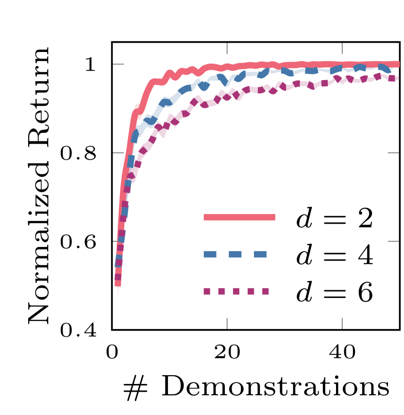
(b) $n=12$ constraints

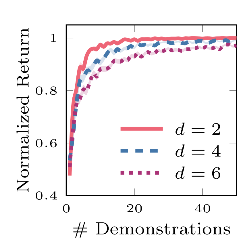
(c) $n=16$ constraints

Figure 8: Return achieved by CoCoRL in single-state CMDPs for different dimensions $d$ and numbers of constraints $n$. We plot the mean and standard errors over $100$ random seeds, although the standard errors are nearly $0$ everywhere. As expected, we need more demonstrations to approximate the true safe set well in higher dimensional feature spaces. There is no noticeable difference in sample complexity for different numbers of constraints. All solutions returned by CoCoRL are safe.

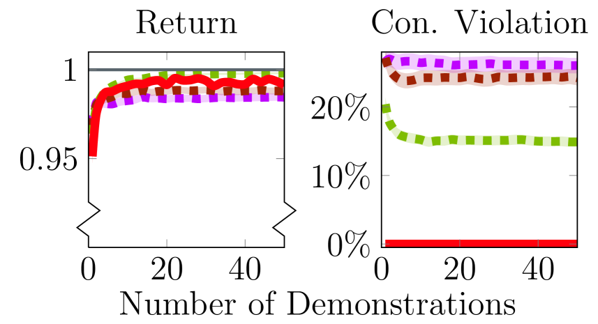
(a) Single environment.

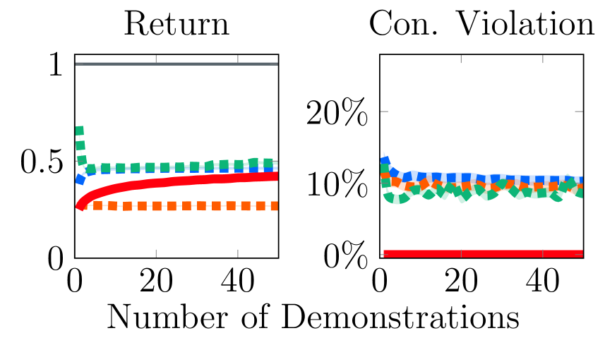
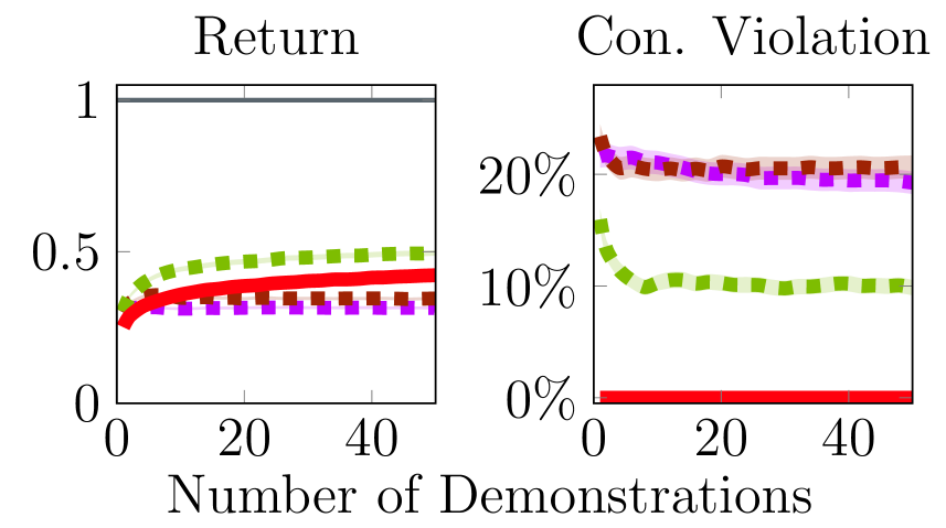
(b) Transfer to new task.

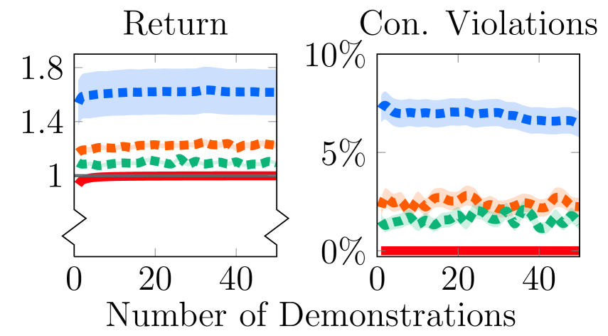
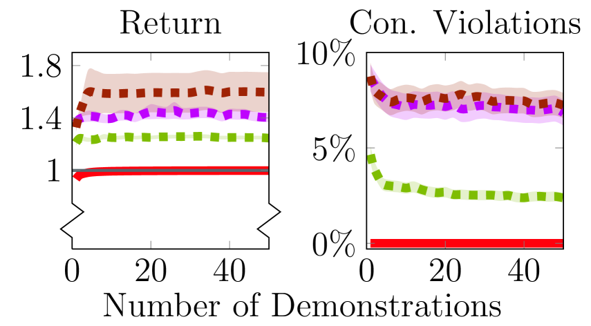
(c) Transfer to new environment.

Figure 9: Experimental results in Gridworld environments, with additional maximum margin IRL baselines. The top row of plots is the same as Figure 2 in the main paper showing CoCoRL compared to the maximum entropy IRL baselines. The bottom row of plots shows CoCoRL compared to the maximum-margin IRL baselines (Section E.1). The plots show mean and standard errors over 100 random seeds. The results are qualitatively similar: the IRL baselines are not safe and can return poor solutions. The maximum margin IRL baselines are slightly better than the maximum entropy IRL baselines. in terms of return but worse in terms of safety.

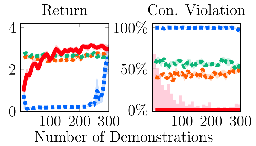
(a) Single environment.

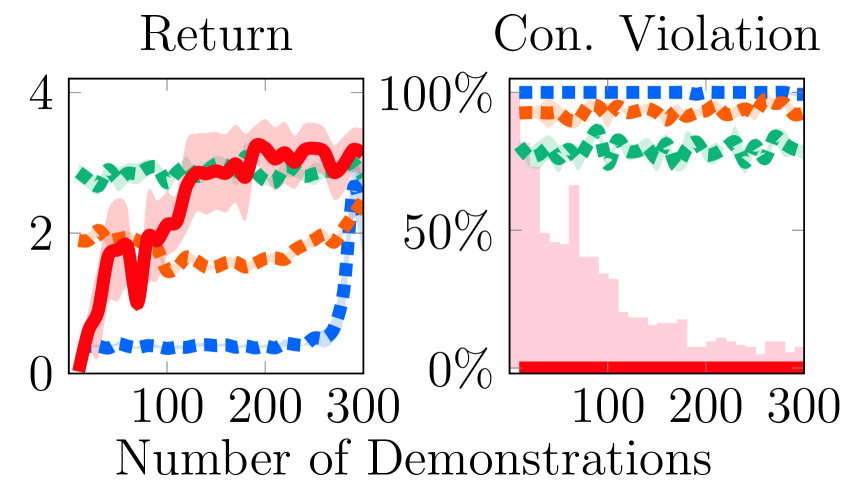
(b) Transfer to new task.

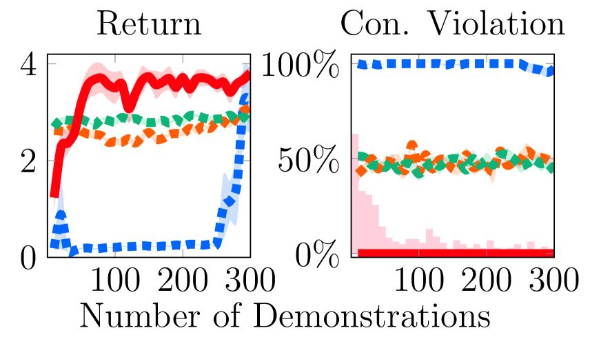
(c) Transfer to new environment.

Figure 10: Experimental results in the highway-env intersection environment, with all IRL baselines. The plots are similar to Figure 4 in the main paper, but, in addition to Known Reward IRL, we show Average IRL and Shared Reward IRL (all based on maximum entropy IRL). All plots show mean and standard error over $5$ random seeds with a fixed set of evaluation rewards for each setting. All baselines fail to return safe solutions and only outperform CoCoRL by violating constraints. Average IRL performs much worse than the other two methods, likely because it assumes that we can average the inferred rewards to remove the reward’s goal component, which is not true in this environment.

References

- Abbeel and Ng (2004) P. Abbeel and A. Y. Ng. Apprenticeship learning via inverse reinforcement learning. In Proceedings of International Conference on Machine Learning (ICML), 2004.
- Altman (1999) E. Altman. Constrained Markov decision processes, volume 7. CRC press, 1999.
- Babes et al. (2011) M. Babes, V. Marivate, K. Subramanian, and M. L. Littman. Apprenticeship learning about multiple intentions. In Proceedings of International Conference on Machine Learning (ICML), 2011.
- Baddeley et al. (2007) A. Baddeley, I. Bárány, and R. Schneider. Random polytopes, convex bodies, and approximation. Stochastic Geometry: Lectures given at the CIME Summer School held in Martina Franca, Italy, September 13–18, 2004, pages 77–118, 2007.
- Baert et al. (2023) M. Baert, P. Mazzaglia, S. Leroux, and P. Simoens. Maximum causal entropy inverse constrained reinforcement learning. arXiv preprint arXiv:2305.02857, 2023.
- Barber et al. (1996) C. B. Barber, D. P. Dobkin, and H. Huhdanpaa. The quickhull algorithm for convex hulls. ACM Transactions on Mathematical Software (TOMS), 22(4):469–483, 1996.
- Camilleri et al. (2022) R. Camilleri, A. Wagenmaker, J. Morgenstern, L. Jain, and K. Jamieson. Active learning with safety constraints. In Advances in Neural Information Processing Systems, 2022.
- Choi and Kim (2012) J. Choi and K.-E. Kim. Nonparametric Bayesian inverse reinforcement learning for multiple reward functions. In Advances in Neural Information Processing Systems, 2012.
- Chou et al. (2020) G. Chou, N. Ozay, and D. Berenson. Learning constraints from locally-optimal demonstrations under cost function uncertainty. IEEE Robotics and Automation Letters, 5(2):3682–3690, 2020.
- Dimitrakakis and Rothkopf (2012) C. Dimitrakakis and C. A. Rothkopf. Bayesian multitask inverse reinforcement learning. In Recent Advances in Reinforcement Learning: 9th European Workshop, EWRL 2011, Athens, Greece, September 9-11, 2011, Revised Selected Papers 9, pages 273–284. Springer, 2012.
- Edalat et al. (2001) A. Edalat, A. Lieutier, and E. Kashefi. The convex hull in a new model of computation. In Proceedings of the 13th Canadian Conference on Computational Geometry, University of Waterloo, Ontario, Canada, August 13-15, 2001, pages 93–96, 2001.
- Edalat et al. (2005) A. Edalat, A. A. Khanban, and A. Lieutier. Computability in computational geometry. In New Computational Paradigms: First Conference on Computability in Europe, CiE 2005, Amsterdam, The Netherlands, June 8-12, 2005. Proceedings 1, pages 117–127. Springer, 2005.
- Garcıa and Fernández (2015) J. Garcıa and F. Fernández. A comprehensive survey on safe reinforcement learning. Journal of Machine Learning Research, 16(1):1437–1480, 2015.
- Gaurav et al. (2023) A. Gaurav, K. Rezaee, G. Liu, and P. Poupart. Learning soft constraints from constrained expert demonstrations. In International Conference on Learning Representations (ICLR), 2023.
- Glazier et al. (2021) A. Glazier, A. Loreggia, N. Mattei, T. Rahgooy, F. Rossi, and K. B. Venable. Making human-like trade-offs in constrained environments by learning from demonstrations. arXiv preprint arXiv:2109.11018, 2021.
- Gottlieb et al. (2018) L.-A. Gottlieb, E. Kaufman, A. Kontorovich, and G. Nivasch. Learning convex polytopes with margin. In Advances in Neural Information Processing Systems, 2018.
- Khan and Madden (2014) S. S. Khan and M. G. Madden. One-class classification: taxonomy of study and review of techniques. The Knowledge Engineering Review, 29(3):345–374, 2014.
- Knox et al. (2023) W. B. Knox, A. Allievi, H. Banzhaf, F. Schmitt, and P. Stone. Reward (mis) design for autonomous driving. Artificial Intelligence, 316:103829, 2023.
- Krajewski et al. (2018) R. Krajewski, J. Bock, L. Kloeker, and L. Eckstein. The highD dataset: A drone dataset of naturalistic vehicle trajectories on German highways for validation of highly automated driving systems. In 2018 21st International Conference on Intelligent Transportation Systems (ITSC), pages 2118–2125, 2018. doi: 10.1109/ITSC.2018.8569552.
- Krakovna et al. (2020) V. Krakovna, J. Uesato, V. Mikulik, M. Rahtz, T. Everitt, R. Kumar, Z. Kenton, J. Leike, and S. Legg. Specification gaming: the flip side of ai ingenuity. DeepMind Blog, 2020. https://www.deepmind.com/blog/specification-gaming-the-flip-side-of-ai-ingenuity.
- Leike et al. (2018) J. Leike, D. Krueger, T. Everitt, M. Martic, V. Maini, and S. Legg. Scalable agent alignment via reward modeling: a research direction. arXiv preprint arXiv:1811.07871, 2018.
- Leurent (2018) E. Leurent. An environment for autonomous driving decision-making. https://github.com/eleurent/highway-env, 2018.
- Leurent et al. (2018) E. Leurent, Y. Blanco, D. Efimov, and O.-A. Maillard. Approximate robust control of uncertain dynamical systems. In Advances in Neural Information Processing Systems, 2018.
- Lindner et al. (2022) D. Lindner, S. Tschiatschek, K. Hofmann, and A. Krause. Interactively learning preference constraints in linear bandits. In Proceedings of International Conference on Machine Learning (ICML), 2022.
- Liu et al. (2023) G. Liu, Y. Luo, A. Gaurav, K. Rezaee, and P. Poupart. Benchmarking constraint inference in inverse reinforcement learning. In International Conference on Learning Representations (ICLR), 2023.
- Malik et al. (2021) S. Malik, U. Anwar, A. Aghasi, and A. Ahmed. Inverse constrained reinforcement learning. In Proceedings of International Conference on Machine Learning (ICML), 2021.
- McMullen (1970) P. McMullen. The maximum numbers of faces of a convex polytope. Mathematika, 17(2):179–184, 1970.
- McPherson et al. (2021) D. L. McPherson, K. C. Stocking, and S. S. Sastry. Maximum likelihood constraint inference from stochastic demonstrations. In Conference on Control Technology and Applications (CCTA), 2021.
- Ng et al. (2000) A. Y. Ng, S. Russell, et al. Algorithms for inverse reinforcement learning. In Proceedings of International Conference on Machine Learning (ICML), 2000.
- Papadimitriou et al. (2022) D. Papadimitriou, U. Anwar, and D. S. Brown. Bayesian inverse constrained reinforcement learning. In Transactions on Machine Learning Research (TMLR), 2022.
- Pulleyblank (1983) W. R. Pulleyblank. Polyhedral combinatorics. Springer, 1983.
- Puterman (1990) M. L. Puterman. Markov decision processes. Handbooks in operations research and management science, 2:331–434, 1990.
- Rezaee and Yadmellat (2022) K. Rezaee and P. Yadmellat. How to not drive: Learning driving constraints from demonstration. In 2022 IEEE Intelligent Vehicles Symposium (IV), 2022.
- Rubinstein and Kroese (2004) R. Y. Rubinstein and D. P. Kroese. The cross-entropy method: a unified approach to combinatorial optimization, Monte-Carlo simulation, and machine learning, volume 133. Springer, 2004.
- Scobee and Sastry (2020) D. R. Scobee and S. S. Sastry. Maximum likelihood constraint inference for inverse reinforcement learning. In International Conference on Learning Representations (ICLR), 2020.
- Sember (2011) J. Sember. Guarantees concerning geometric objects with imprecise points. PhD thesis, University of British Columbia, 2011.
- Stocking et al. (2021) K. C. Stocking, D. L. McPherson, R. P. Matthew, and C. J. Tomlin. Discretizing dynamics for maximum likelihood constraint inference. arXiv preprint arXiv:2109.04874, 2021.
- Wang et al. (2021) P. Wang, H. Li, and C.-Y. Chan. Meta-adversarial inverse reinforcement learning for decision-making tasks. In International Conference on Robotics and Automation (ICRA), 2021.
- Wen and Topcu (2018) M. Wen and U. Topcu. Constrained cross-entropy method for safe reinforcement learning. In Advances in Neural Information Processing Systems, 2018.
- Xu et al. (2019) K. Xu, E. Ratner, A. Dragan, S. Levine, and C. Finn. Learning a prior over intent via meta-inverse reinforcement learning. In Proceedings of International Conference on Machine Learning (ICML), 2019.
- Yu et al. (2019) L. Yu, T. Yu, C. Finn, and S. Ermon. Meta-inverse reinforcement learning with probabilistic context variables. In Advances in Neural Information Processing Systems, 2019.
- Ziebart et al. (2008) B. D. Ziebart, A. L. Maas, J. A. Bagnell, A. K. Dey, et al. Maximum entropy inverse reinforcement learning. In AAAI Conference on Artificial Intelligence, 2008.