OU-HEP-230501

On practical naturalness and its implications
for weak scale supersymmetry

Howard Baer¹, Vernon Barger², Dakotah Martinez¹ and Shadman Salam^3
1Homer L. Dodge Department of Physics and Astronomy,
University of Oklahoma, Norman, OK 73019, USA
²Department of Physics, University of Wisconsin, Madison, WI 53706 USA
³Center for Mathematical Sciences, Department of Mathematics and Natural Sciences, Brac University, Dhaka 1212, Bangladesh

We revisit the various measures of naturalness for models of weak scale supersymmetry including 1. electroweak (EW) naturalness, 2. naturalness via sensitivity to high scale parameters (EENZ/BG), 3. sensitivity of Higgs soft term due to high scale (HS) radiative corrections and 4. stringy naturalness (SN) from the landscape. The EW measure is most conservative and seems unavoidable; it is also model independent in that its value is fixed only by the weak scale spectra which ensues, no matter which model is used to generate it. The EENZ/BG measure is ambiguous depending on which “parameters of ignorance” one includes in the low energy effective field theory (LE-EFT). For models with calculable soft breaking terms, then the EENZ/BG measure reduces to the tree-level EW measure. The HS measure began life as a figurative expression and probably shouldn’t be taken more seriously than that. SN is closely related to EW naturalness via the atomic principle, although it is also sensitive to the distribution of soft terms on the landscape. If the landscape favors large soft terms, as in a power law distribution, then it favors $m_{h}\simeq 125$ GeV along with sparticles beyond present LHC reach. In this context, SN appears as a probability measure where more natural models are expected to be more prevalent on the landscape than finetuned models. We evaluate by how much the different measures vary against one another with an eye to determining by how much they may overestimate finetuning; we find overestimates can range up to a factor of over 1000. In contrast to much of the literature, we expect the string landscape to favor EW natural SUSY models over finetuned models so that the landscape is not an alternative to naturalness.

1 Introduction

Weak scale supersymmetry provides a very clean solution to the hierarchy of scales problem[1, 2] of particle physics and is actually supported by data from four different virtual effects:

1. the successful running of gauge couplings to unified values within the Minimal Supersymmetric Standard Model (MSSM)[3, 4, 5, 6],

2. the predicted large value of the top quark mass needed for radiatively-induced electroweak symmetry breaking (REWSB)[7, 8, 9],

3. the match between the narrow theory-predicted window of $m_{h}$ values within the MSSM and the subsequent Higgs boson discovery[10] and

4. precision electroweak corrections which, in the $m_{t}$ vs. $m_{W}$ plane, actually favor heavy SUSY over the SM[11].

In addition, some remnant SUSY is expected to survive superstring compactification from 10/11 to four spacetime dimensions on a Calabi-Yau manifold[12]. In fact, it is conjectured that the landscape of all geometric, stable, string/M theory compactifications to Minkowski spacetime (at leading order) are supersymmetric[13]; manifolds which do not respect these conditions typically lead to Witten bubble-of-nothing instabilities. Also, in contrast to the SM, SUSY leads to EW vacuum stability at ultra-high energies owing to gauge sector contributions (D-terms) to Higgs quartic couplings[14]. Plus, highly motivated SM extensions which introduce a new high energy scale– such as the inclusion of see-saw neutrinos or a Peccei-Quinn sector to solve the strong CP problem– avoid the Higgs mass blow-up due to the introduced new high mass scales[15, 16, 17] unless the underlying model is supersymmetric. And with respect to the axion solution to the strong CP problem, intrinsically supersymmetric discrete $R$-symmetries[18], which are expected to emerge from string compactifications[19], provide an avenue for emergence of the required global $U(1)_{PQ}$ symmetry with sufficient precision as to solve the axion quality problem[20, 21]. In such models, the PQ scale $f_{a}$ is related to the hidden sector SUSY breaking scale $m_{hidden}\sim f_{a}\sim 10^{11}$ GeV so that $f_{a}$ lies within the cosmological sweet spot for axion production via coherent oscillations in the early universe[20]. String instanton effects on the axion quality are also ameliorated within the MSSM[22]. And while there are few compelling mechanisms for successful baryogenesis left within the rubric of the SM, the introduction of SUSY leads to several new and/or improved mechanisms to address the matter-antimatter asymmetry[23, 24].

In spite of this impressive litany of successes, it is common nowadays to dismiss weak scale supersymmetry (WSS)[25] as a viable beyond-the-Standard Model (BSM) theory due to the apparent lack of new physics signals at the CERN Large Hadron Collider (LHC)[26]. The data from LHC, which is by-and-large in accord with SM expectations[27], is in contrast to early theoretical expectations for WSS based upon naturalness arguments that superpartners would emerge with mass values not far from the weak scale $m_{weak}\simeq m_{W,Z,h}\sim 100$ GeV[28, 29, 30, 31, 32, 33, 34, 35, 36]. At present, such arguments are being used to set policy and guide future facilities for the High Energy Physics (HEP) frontier[37, 38]. Given the stakes involved, it is essential to go back and review the naturalness-based arguments to assess when and where and if they present a reliable guide to the search for new physics. After all, the original naturalness arguments are over 30 years old, and the HEP community has hopefully learned a lot since then.

In this paper, we revisit several proposed naturalness measures which have been applied to various supersymmetric models. As opposed to ’t Hooft naturalness, these measures determine the degree of what is defined in Sec. 3 as practical naturalness: that all independent contributions to some observable $\cal{O}$ are comparable to or less than $\cal{O}$. Historically, the first of these is the EENZ/BG[28, 29] measure (labeled here as $\Delta_{\rm BG}$) which determines the sensitivity of the measured value of the weak scale to variation in model parameters $p_{i}$ ($i$ labels the various parameters under consideration). Typically the $p_{i}$ have been taken to be the various soft SUSY breaking terms starting at a high effective field theory (EFT) cutoff scale $\Lambda=m_{GUT}\simeq 2\times 10^{16}$ GeV:

$$\Delta_{\rm BG}\equiv max_{i}|\frac{\partial\log m_{Z}^{2}}{\partial\log p_{i}}|=max_{i}|\frac{p_{i}}{m_{Z}^{2}}\frac{\partial m_{Z}^{2}}{\partial p_{i}}|.$$ (1)

For small $\Delta_{\rm BG}\lesssim 30$, then sparticle masses are expected below the several hundred GeV range although in some special regions of model parameter space, such as the focus point region[39, 40] of the minimal supergravity[41] (mSUGRA) or constrained MSSM[42] (CMSSM) model, multi-TeV scale top squarks can be allowed. Despite its popularity, this measure has been argued to overestimate finetuning in SUSY models by large factors and to give ambiguous answers depending on exactly which parameters are chosen to be the fundamental $p_{i}$[43, 44].

A second measure, which we label here as $\Delta_{\rm HS}$ (for high scale sensitivity of the up-Higgs soft mass $m_{H_{u}}^{2}$), starts with the approximate SUSY Higgs mass relation $m_{h}^{2}\sim\mu^{2}+m_{H_{u}}^{2}(weak)$ where $m_{H_{u}}^{2}(weak)=m_{H_{u}}^{2}(\Lambda)+\delta m_{H_{u}}^{2}$. One then requires

$$\Delta_{\rm HS}=\delta m_{H_{u}}^{2}/m_{h}^{2}$$ (2)

to be small. (As mentioned earlier, it is the large top-quark Yukawa coupling $f_{t}$ which radiatively drives $m_{H_{u}}^{2}$ from its large SUGRA value at the high scale to negative values at the weak scale so that EW symmetry is spontaneously broken.) This measure, which is inconsistent with $\Delta_{\rm BG}$ in that it doesn’t allow for multi-TeV top squarks even in the FP region, has lead to intense scrutiny of LHC top squark searches since it is expected that $\delta m_{H_{u}}^{2}\sim\frac{6f_{t}^{2}}{(4\pi)^{2}}m_{\tilde{t}}^{2}\log\frac{\Lambda^{2}}{m_{\tilde{t}}^{2}}$[45, 46, 47, 48, 49, 50, 51]. $\Delta_{\rm HS}$ was found to lead to violations of the finetuning rule[43]: that it is not allowed to claim finetuning amongst dependent terms which contribute to some observable ${\cal O}$. In this case, $\delta m_{H_{u}}^{2}$ and $m_{H_{u}}^{2}(\Lambda)$ are dependent, leading to overestimates in finetuning.

A third measure is the electroweak measure $\Delta_{\rm EW}$[52, 53] which is touted to be more conservative and model independent than the others, and also unavoidable (within the context of the MSSM). It is based on the SUSY Higgs potential minimization condition

$$m_{Z}^{2}/2=\frac{m_{H_{d}}^{2}+\Sigma_{d}^{d}-(m_{H_{u}}^{2}+\Sigma_{u}^{u})\tan^{2}\beta}{\tan^{2}\beta-1}-\mu^{2}\simeq-m_{H_{u}}^{2}-\mu^{2}-\Sigma_{u}^{u}(\tilde{t}_{1,2})$$ (3)

where all right-hand-side (RHS) entries are taken as their weak scale values and

$$\Delta_{\rm EW}\equiv max_{i}|entries\ on\ RHS\ of\ Eq.\ \ref{eq:mzs}|/(m_{Z}^{2}/2).$$ (4)

This measure was preceded by Chan et al.[54] who suggested that the magnitude of the SUSY conserving $\mu$ parameter could serve as a finetuning measure all by itself. This measure is sometimes criticized in that it apparently lacks sensitivity to high scale parameters (more on this later).

A fourth entry is not at present a quantifiable measure, but known nonetheless as stringy naturalness (SN), and arises from Douglas’ consideration of the string landscape picture[55]:

Stringy naturalness: An observable ${\cal O}_{1}$ is more (stringy) natural than observable ${\cal O}_{2}$ if more phenomenologically viable string vacua lead to ${\cal O}_{1}$ than to ${\cal O}_{2}$.

To quantify stringy naturalness, at least two ingredients are needed: 1. the expected distribution of some quantity within the landscape of vacua possibilities and 2. an anthropic selection ansatz for which many choices would lead to universes that are unable to support observers. For the case of SUSY models, the first of these is usually how soft terms are distributed in the landscape while the second of these is the magnitude of the weak scale itself: if the predicted value of $m_{weak}$ within each pocket universe is too far displaced from its measured value in our universe, then nuclear physics goes astray, and atoms as we know them fail to appear– leading to no complex chemistry as seems to be needed for life as we know it (atomic principle)[56]. An attempt to compute and display stringy naturalness via density of dots in model parameter space has been made in Ref. [57].

In the present work, we reexamine these several measures of naturalness, filling in some of the many gaps of understanding that exist in the literature. Part of our work is based on a new computation of $\Delta_{\rm BG}$ naturalness based on evaluating numerically the derivatives in Eq. 1. This new computation is embedded in the publicly available code DEW4SLHA[53] so that the updated code can provide values of each of the measures $\Delta_{\rm BG}$, $\Delta_{\rm HS}$ and $\Delta_{\rm EW}$ given an input SUSY Les Houches Accord (SLHA) file[58]. We also compute ratios of naturalness measures to determine the extent of which some measures can overestimate finetuning in SUSY models. For instance, in the SUSY theory review contained in the Particle Data Book[59], it is suggested that the overestimates may range up to a factor 10; in contrast, we find overestimates ranging up to factors of over 1000.

2 Some models of weak scale SUSY

In our deliberations, we make reference to several SUSY models which we briefly review here for the reader.

2.1 mSUGRA/CMSSM model

Some of our numerical work refers to the mSUGRA[41] or CMSSM model[42] with parameter space

$$m_{0},\ m_{1/2},\ A_{0},\ \tan\beta\ \ {\rm and}\ \ {\rm sign}(\mu)\ \ \ ({\rm mSUGRA/CMSSM}).$$ (5)

In this model, $m_{0}$ refers to a unified high scale scalar soft breaking mass, usually defined at the scale $m_{GUT}$ where the three gauge couplings unify. While unified gaugino masses can be developed in many supersymmetric models with a simple choice for gauge kinetic function, the scalar mass unification is an (unmotivated) simplifying assumption that violates expectations from gravity-mediated SUSY breaking models where non-universal scalar masses are expected unless imposed by some symmetry[60, 61, 62]. For instance, scalar masses within a matter generation may be expected to unify to $m_{0}(i)$ (for generation index $i=1-3$) due to the fact that all matter fills out a complete 16-dimensional spinor representation of $SO(10)$. However, generational universality $m_{0}(1)=m_{0}(2)=m_{0}(3)$ is not expected and leads to the famous SUSY flavor and CP problems[63]. Furthermore, the Higgs fields $H_{u}$ and $H_{d}$ live in different $SU(5)$ (or general $SO(10)$) representations from matter scalars, and hence are also not expected to unify.

2.2 Non-universal Higgs models (NUHM)

These models come in several different guises and meet the expectation that $m_{H_{u}}\neq m_{H_{d}}\neq m_{0}(i)$. The simplest case, NUHM1[64] assumes $m_{H_{u}}=m_{H_{d}}\neq m_{0}(i)$ as expected in simple $SO(10)$ GUTs, while NUHM2[65, 66, 67] with $m_{H_{u}}\neq m_{H_{d}}\neq m_{0}(i)$ occurs in $SU(5)$ or general $SO(10)$ GUTs. In all cases, when we speak of SUSY GUT models we have an eye towards local grand unification[68] wherein the geography of fields on a string compactified manifold determines the GUT symmetry properties[69, 70]. Sometimes an NUHM3 model with $m_{0}(1)=m_{0}(2)\neq m_{0}(3)$ is used[71] and sometimes NUHM4 with $m_{0}(1)\neq m_{0}(2)\neq m_{0}(3)$ is used especially for discussion of the SUSY flavor and CP problems[72]. For these NUHMi models ($i=1-4$), frequently the GUT values of $m_{H_{u}}$ and $m_{H_{d}}$ are traded for the weak scale values of the superpotential $\mu$ parameter and the pseudoscalar Higgs mass $m_{A}$ via the scalar potential minimization conditions. Thus, the NUHMi parameter space is given by

$$m_{0}(i),\ m_{1/2},\ A_{0},\ \tan\beta,\ \mu,\ m_{A}.$$ (6)

The NUHMi models are particularly convenient to explore natural supersymmetry since one can directly restrict oneself to natural values of the $\mu$ parameter: $\mu\sim 100-350$ GeV.

In Fig. 1, we plot in the $m_{0}$ vs. $m_{1/2}$ plane of the NUHM2 model the ratio of $m_{H_{u}}(m_{GUT})/m_{0}$ which is needed to ensure that the SUSY $\mu$ parameter is fixed at a natural value of $\mu=200$ GeV. We also adopt $A_{0}=-1.6m_{0}$ and $\tan\beta=10$ with $m_{A}=2$ TeV. From the plot, we see that $m_{H_{u}}(m_{GUT})\sim 2m_{0}$ along the left-hand-side of the plot, but dips to a ratio of about 1.2-1.5 for the bulk of the plane which respects the $m_{h}\sim 123-127$ GeV range (assuming about a 2 GeV error bar on the $m_{h}$ theory calculation). Thus, only modest deviations of order 20-50% are required in order ensure one of the most fundamental requirements of naturalness, namely $|\mu|\sim m_{weak}$.

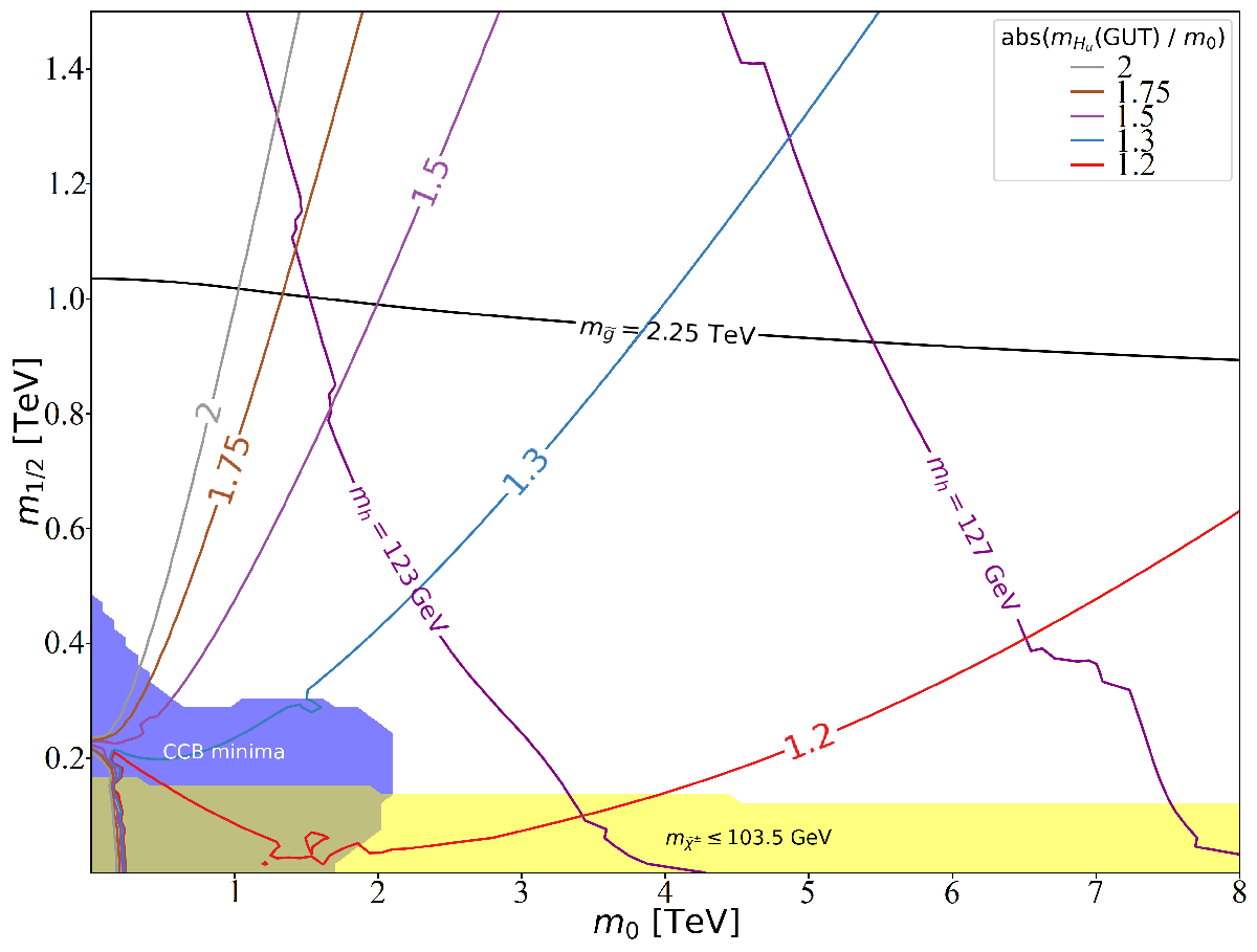
Figure 1: Ratio of $m_{H_{u}}(m_{GUT})/m_{0}$ in the NUHM2 model which is needed to ensure that $\mu=200$ GeV. We also take $A_{0}=-1.6m_{0}$ and $\tan\beta=10$ with $m_{A}=2$ TeV. The blue shaded region is excluded, as these points lead to CCB minima. The yellow shaded region near the bottom has the lightest chargino below LEP2 limits, $m_{\widetilde{\chi}_{1}^{\pm}}<103.5$ GeV. The spectra is calculated using SoftSUSY.

2.3 Natural anomaly and mirage mediation models

Later in this paper we shall explore naturalness in the guise of anomaly-mediated SUSY breaking (AMSB)[73, 74, 75] and mixed modulus-AMSB SUSY models, also known as mirage mediation (MM)[76, 77].

3 Naturalness and practical naturalness

Supersymmetry offers a ’t Hooft technically natural solution[78] to the hierarchy of scales problem in that, as the hidden sector SUSY breaking scale $m_{hidden}$ (which determines the magnitude of the soft terms via $m_{soft}\sim m_{3/2}\sim m_{hidden}^{2}/m_{P}$ in gravity-mediation and hence of the weak scale via the scalar potential minimization conditions) is taken to zero, the model becomes more (super)symmetric. The SUSY solution to this big hierarchy problem (BHP)– stabilizing the weak scale so that it doesn’t blow up to the Planck or GUT scale– is not the naturalness issue which concerns many contemporary SUSY theorists. Indeed, ’t Hooft naturalness remains a valid solution to the BHP even for very large gaps $m_{soft}\gg m_{weak}$. Instead, it is the so-called little hierarchy problem (LHP) which is of concern[79, 80]:

how can it be that $m_{weak}\sim m_{W,Z,h}\sim 100$ GeV is so much smaller than the soft SUSY breaking terms, which– according to LHC data– are $m_{soft}\gtrsim 1$ TeV (owing to LHC bounds $m_{\tilde{g}}\gtrsim 2.2$ TeV, $m_{\tilde{t}_{1}}\gtrsim 1.1$ TeV, $\cdots$)[81].

In addressing the LHP, what is of concern is what we call the notion of practical naturalness (PN)[82]:

An observable ${\cal O}=o_{1}+\cdots+o_{n}$ is practically natural if all independent contributions $o_{i}$ to ${\cal O}$ are comparable to or less than ${\cal O}$.

(Here, comparable to means within a factor of several from the measured value.) Practical naturalness embodies the notion of naturalness that is most often used in successful applications of naturalness. For instance, by requiring the charm quark mass contribution

$$\Delta m_{K}(c)\simeq\frac{G_{F}}{\sqrt{2}}\frac{\alpha}{6\pi}\frac{f_{K}^{2}m_{K}}{\sin^{2}\theta_{W}}\cos^{2}\theta_{C}\sin^{2}\theta_{C}\frac{m_{c}^{2}}{m_{W}^{2}}$$ (7)

to be comparable to or less than the measured $K_{L}-K_{S}$ mass difference $\Delta m_{K}$, Gaillard and Lee[85] were able to predict $m_{c}\sim 1.5$ GeV several months before the charm quark was discovered. An essential element of practical naturalness is that the contributions $o_{i}$ should be independent of one another in the sense that if one of the $o_{i}$ is varied, then the others don’t necessarily vary. For instance, Dirac was bothered by various divergent contributions to perturbative QED observables. However, these were dependent contributions in that if the regulator was varied, the different divergent terms would also vary. One should always first combine dependent terms before evaluating naturalness. Once dependent terms are combined, then a measure of naturalness emerges:

$$\Delta\equiv max_{i}|o_{i}|/|{\cal O}|.$$ (8)

Using PN, we see that QED perturbation theory is practically natural in that the leading terms are comparable to the measured observables whilst higher order terms (once dependent terms are combined) are typically much smaller.

4 Some measures of naturalness

4.1 Sensitivity to high scale parameters: EENZ/BG naturalness

Historically, the first measure of SUSY model naturalness was proposed by Ellis et al. in Ref. [28] and subsequently used by Barbieri and Giudice[29] to compute sparticle mass upper bounds in the mSUGRA/CMSSM model: Eq. 1. The measure purports to compute sensitivity of the measured value of the weak scale to variation in high scale parameters $p_{i}$. The $\Delta_{\rm BG}$ measure is actually a measure of practical naturalness of the weak scale in the case where $m_{Z}^{2}=a_{1}p_{1}+\cdots a_{n}p_{n}$. Let’s suppose the $j$th contribution to $m_{Z}^{2}$ is largest. Then $\Delta_{\rm BG}=max_{i}|(p_{i}/m_{Z}^{2})\partial m_{Z}^{2}/\partial p_{i}|=|a_{j}p_{j}/m_{Z}^{2}|$ in accord with Eq. 8. The various $|a_{i}p_{i}/m_{Z}^{2}|\equiv c_{i}$ terms are labeled sensitivity coefficients[86]. The rub here is what choice to take as to the free parameters $p_{i}$.

The starting point is to express $m_{Z}^{2}$ in terms of weak scale SUSY parameters as in Eq. 3:

$$m_{Z}^{2}\simeq-2m_{H_{u}}^{2}-2\mu^{2}$$ (9)

where the partial equality obtains for moderate-to-large $\tan\beta$ values and where we assume for now that the radiative corrections are small. To evaluate $\Delta_{BG}$, one needs to know the explicit dependence of $m_{H_{u}}^{2}$ and $\mu^{2}$ on the fundamental parameters. Semi-analytic solutions to the one-loop renormalization group equations for $m_{H_{u}}^{2}$ and $\mu^{2}$ can be found for instance in Refs. [88, 89]. For the case of $\tan\beta=10$, then[36, 90, 86]

$$m_{Z}^{2} \simeq -2.18\mu^{2}+3.84M_{3}^{2}+0.32M_{3}M_{2}+0.047M_{1}M_{3}$$ (10)

$$-0.42M_{2}^{2}+0.011M_{2}M_{1}-0.012M_{1}^{2}-0.65M_{3}A_{t}$$

$$-0.15M_{2}A_{t}-0.025M_{1}A_{t}+0.22A_{t}^{2}+0.004M_{3}A_{b}$$

$$-1.27m_{H_{u}}^{2}-0.053m_{H_{d}}^{2}$$

$$+0.73m_{Q_{3}}^{2}+0.57m_{U_{3}}^{2}+0.049m_{D_{3}}^{2}-0.052m_{L_{3}}^{2}+0.053m_{E_{3}}^{2}$$

$$+0.051m_{Q_{2}}^{2}-0.11m_{U_{2}}^{2}+0.051m_{D_{2}}^{2}-0.052m_{L_{2}}^{2}+0.053m_{E_{2}}^{2}$$

$$+0.051m_{Q_{1}}^{2}-0.11m_{U_{1}}^{2}+0.051m_{D_{1}}^{2}-0.052m_{L_{1}}^{2}+0.053m_{E_{1}}^{2},$$

where all terms on the right-hand-side are understood to be $GUT$ scale parameters. As an example, if we adopt $m_{Q_{3}}^{2}$ as a fundamental parameter, then the sensitivity coefficient $c_{m_{Q_{3}}^{2}}=0.73m_{Q_{3}}^{2}/m_{Z}^{2}$ and for $m_{Q_{3}}=3$ TeV, then one finds $c_{m_{Q_{3}}^{2}}\simeq 800$ so that $\Delta_{\rm BG}>800$ and the model is certainly finetuned. If instead we declare all scalar masses unified to $m_{0}$, then there are large cancellations and instead one finds $c_{m_{0}^{2}}=0.013m_{0}^{2}/m_{Z}^{2}\sim 14.2$: a reduction in finetuning by over a factor 50! Clearly, whether or not soft terms are correlated or not makes a big difference in the evaluation of $\Delta_{\rm BG}$!

4.1.1 Numerical routine to compute $\Delta_{\rm BG}$

The evaluation of $\Delta_{BG}$ can be done by approximating the partial derivatives with the method of two-point finite central difference quotients. That is, for finding the partial derivative with respect to a parameter $p_{1}$ of $m_{Z}^{2}(p_{1},p_{2},\ldots,p_{n})$, where $p_{i}$ are the fundamental parameters of the model chosen for evaluating $\Delta_{BG}$, then

$$\frac{\partial m_{Z}^{2}\left(p_{1},p_{2},\ldots,p_{n}\right)}{\partial p_{1}}\approx\frac{m_{Z}^{2}(p_{1}+h_{1},p_{2},\ldots,p_{n})-m_{Z}^{2}(p_{1}-h_{1},p_{2},\ldots,p_{n})}{2h_{1}}.$$ (11)

$h_{1}$ is the size of the variation of the differentiation parameter $p_{1}$, which is then used to determine the resulting change in $m_{Z}^{2}$. Since this is a partial derivative, all other input parameters are left fixed at their original values prior to differentiation.

To compute this derivative, $m_{Z}^{2}$ must be evaluated in the right-hand side of Eq. 11 as an output of the $m_{Z}^{2}$ Higgs minimization condition, Eq. 3, at the weak renormalization scale $Q_{\text{SUSY}}=\sqrt{m_{\widetilde{t}_{1}}m_{\widetilde{t}_{2}}}$ to minimize radiative corrections in the Higgs minimization condition. For the partial derivative of $m_{Z}^{2}$ with respect to $p_{i}$, the GUT-scale parameter $p_{i}$ defined at the renormalization scale $Q_{\text{GUT}}$ is varied to $p_{i}+h_{i}$, with $h_{i}\ll p_{i}$. Then the new set of GUT-scale parameters $\{p_{1},p_{2},\ldots,p_{i}+h_{i},\ldots,p_{n-1},p_{n}\}$ are evolved from $Q_{\text{GUT}}$ down to $Q_{\text{SUSY}}$ using the full two-loop MSSM renormalization group equations (RGEs). Lastly, the varied value $m_{Z}^{2}(p_{1},p_{2},\ldots,p_{i}+h_{i},\ldots,p_{n-1},p_{n})$ is computed from the tree-level Higgs minimization condition for $m_{Z}^{2}$, giving a value slightly deviated from $91.2^{2}$. This value is then used in Eq. 11 and the process is repeated for the other direction of variation.

In this numerical derivative approach, two sources of error can enter and skew the results: truncation error and roundoff error. Below are some descriptions of these errors and how we minimize them.

• Truncation error is the error of approximating the true, analytical derivative of $m_{Z}^{2}$, a tangent line to the $m_{Z}^{2}$ curve, with our numerical two-point method, producing a secant line to the $m_{Z}^{2}$ curve. For a given derivative variation size of $h$, the truncation error for this two-point method is suppressed by a term of $\mathcal{O}(h^{2})$. This error remains relatively small so long as the step size $h<1$ and the higher-order derivatives of $m_{Z}^{2}$ are reasonably bounded.

• Roundoff error comes from representing the values $p_{1},p_{2},\ldots,p_{n},$ and $h_{1}$ in Eq. 11 as floating point numbers, where the computer must “round off” most decimal values after a certain number of digits due to storage limitations in binary. Because of this, there is a non-zero spacing between two consecutive floating point numbers $x$ and $y$, and this spacing is called the unit of least precision (denoted ULP($x$)). Careful error analysis reveals that the roundoff error is proportional to the step size used in the evaluation. This roundoff error is then minimized when, for a two-point central difference, the step size $h_{i}$ for the derivative with respect to some $p_{i}$ is chosen as $h_{i}\approx\left[\text{ULP}\left(p_{i}\right)\right]^{1/3}$. In order for $h_{i}<1$ to occur, the ULP$\left(p_{i}\right)$ must then also be less than unity.

Numerical error may also enter through the numerical solution of the RGEs, though similar numerical considerations can help control these errors as well. With these sources of error in mind, the error in evaluating this derivative will remain small, i.e., $\mathcal{O}(<1)$, so long as $|p_{i}|\lesssim 10^{15}$ in magnitude for all $i$. This leads to $h_{i}<1$ for double-precision floating point numbers. DEW4SLHA offers the option of performing this calculation with even higher accuracy derivative approximations, such as a four-point or eight-point central difference quotient to further minimize truncation error.

The numerical evaluation of $\Delta_{\rm BG}$ has several advantages over the semi-analytic formulae using expansions such as Eq. 10.

• The numeric routine uses full two-loop RGEs including all third generation Yukawa couplings[91] and one loop threshold effects while semi-analytic expansions use one-loop RGEs without threshold effects.

• The semi-analytic expansions were formulated to compute the Higgs potential at a scale $Q\sim m_{Z}$ whilst the numeric routine uses an optimized scale choice $Q^{2}=m_{\tilde{t}_{1}}m_{\tilde{t}_{2}}$ which matches the higher scales for MSSM/SM decoupling that are expected from LHC data.

• Usually the semi-analytic expansions are computed for a particular $\tan\beta$ value while the numeric evaluation is valid for all $\tan\beta$.

To illustrate the comparison between the two methods, in Fig. 2a) we compute the ratio $\Delta_{BG}(\text{numerical})/\Delta_{\rm BG}(\text{semianalytic})$ in the $m_{0}$ vs. $m_{1/2}$ plane of the mSUGRA/CMSSM plane for $A_{0}=0$ and $\tan\beta=10$ with $\mu>0$. The blue region corresponds to a ratio $\sim 0.5$ while for small $m_{0}$ we find $\Delta_{BG}(\text{numerical})/\Delta_{\rm BG}(\text{semianalytic})\lesssim 1$ and for large $m_{0}$ then we find $\Delta_{BG}(\text{numerical})/\Delta_{\rm BG}(\text{semianalytic})\gtrsim 1$ with the ratio reaching as high as $\sim 2$ near the lower focus point region.

In Fig. 2b) we again compute the ratio $\Delta_{\rm BG}(\text{numerical})/\Delta_{\rm BG}(\text{semianalytic})$ in the $m_{0}$ vs $m_{1/2}$ plane of the mSUGRA/CMSSM, but now for $A_{0}=-2m_{0}$ and $\tan\beta=10$ with $\mu>0$. The large value of $A_{0}$ here permits the Higgs mass to be within the allowed range of $125\pm 2$ GeV. The broad orange and red regions throughout the RHS of the plane correspond to where $\Delta_{\rm BG}(\text{numerical})\sim\Delta_{\rm BG}(\text{semianalytic})$. The largest discrepancy between the evaluation methods occurs on the LHS of the plane near the stau LSP region, where $\Delta_{\rm BG}(\text{numerical})\sim 0.6\Delta_{\rm BG}(\text{semianalytic})$. Fig. 2c) instead shows the ratio comparing the numerical method to the semianalytic method in the $m_{0}$ vs $m_{1/2}$ plane of the NUHM2 model with $\mu=200$ GeV, $m_{A}=2$ TeV and $A_{0}=-1.6m_{0}$. Again, the broad orange and red region on the RHS of this plane shows very good agreement between the two methods: $\Delta_{\rm BG}(\text{numerical})\sim\Delta_{\rm BG}(\text{semianalytic})$. On the LHS above the CCB minima region, where $m_{1/2}>m_{0}$, then the semianalytic method result becomes somewhat larger than the numerical method result, leading to a minimal ratio $\Delta_{\rm BG}(\text{numerical})\sim 0.57\Delta_{\rm BG}(\text{semianalytic})$.

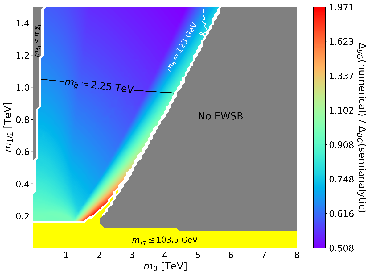
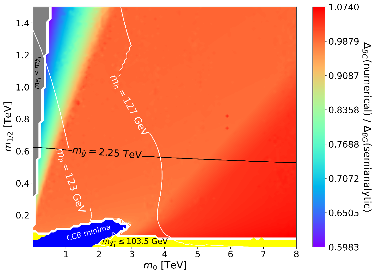
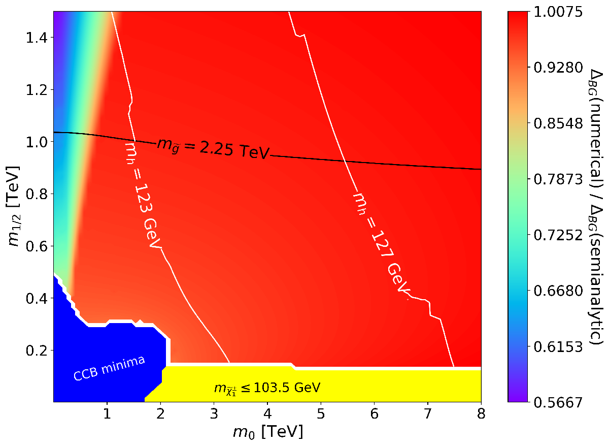
Figure 2: Plot of $\Delta_{BG}(\text{numerical})/\Delta_{\rm BG}(\text{semianalytic})$ in the $m_{0}$ vs. $m_{1/2}$ plane of a) the CMSSM/mSUGRA model with $A_{0}=0$, $\tan\beta=10$ and $\mu>0$, b) the CMSSM/mSUGRA model with $A_{0}=-2m_{0}$ and c) the NUHM2 model with $\mu=200$ GeV and $A_{0}=-1.6m_{0}$ with $m_{A}=2$ TeV. We use the code DEW4SLHA to compute $\Delta_{BG}(\text{numerical})$ using a numerical algorithm for the sensitivity coefficients and SoftSUSY v4.1.17 for the spectrum.

4.1.2 Numerical results for $\Delta_{\rm BG}$

In Fig. 3, we compute contours and color-coded regions of $\Delta_{\rm BG}$ in the mSUGRA/CMSSM model using a numerical routine to evaluate the sensitivity coefficients. This routine is embedded in the publicly available computer code DEW4SLHA which computes the three measures of naturalness $\Delta_{\rm BG}$, $\Delta_{\rm HS}$ and $\Delta_{\rm EW}$ for any model based on its Les Houches Accord spectrum generator output file. The results in Fig. 3 agree well with those presented by Allanach et al. in Ref. [92].

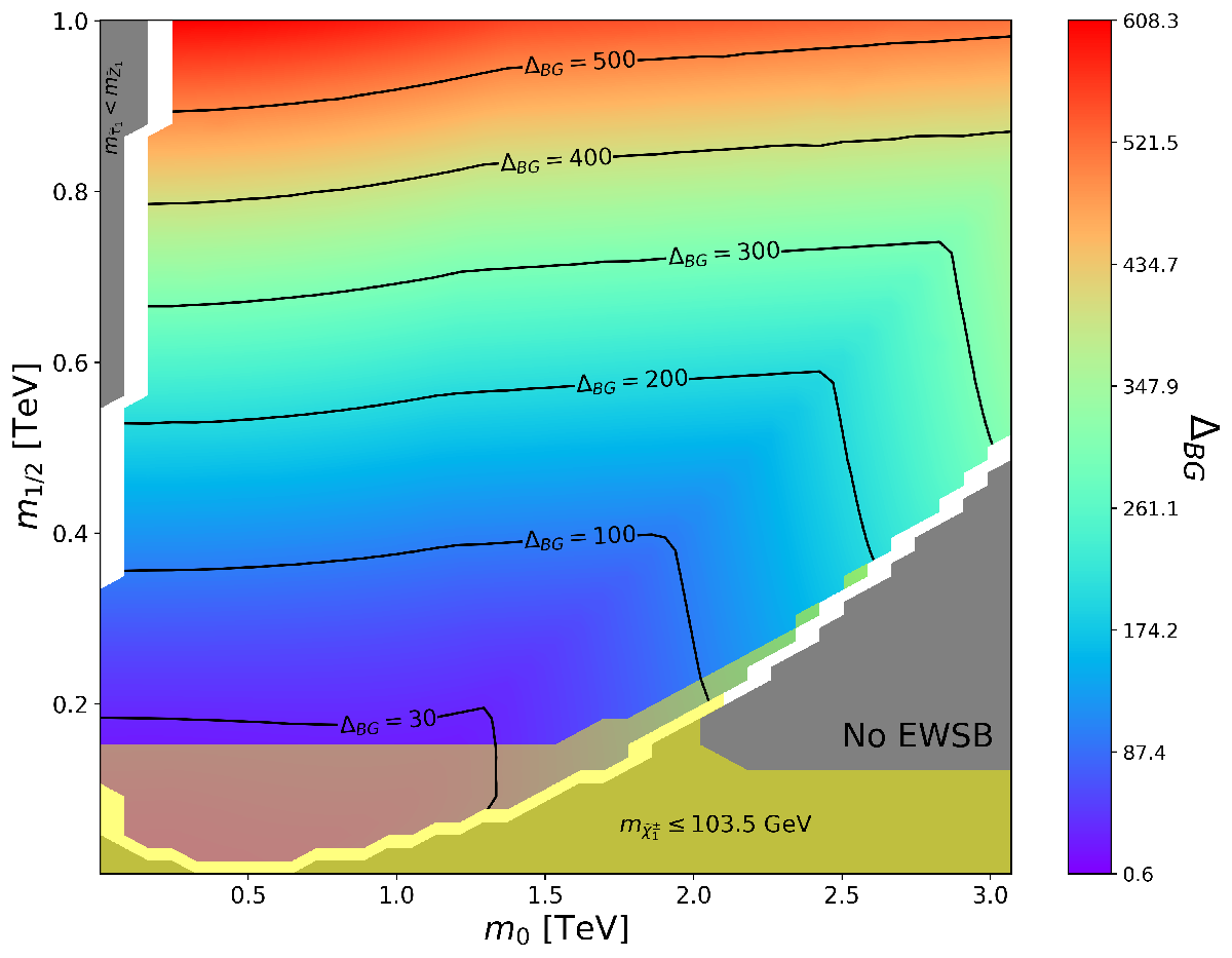
Figure 3: Plot of naturalness contours $\Delta_{BG}$ in the $m_{0}$ vs. $m_{1/2}$ plane of the CMSSM/mSUGRA model with $A_{0}=0$, $\tan\beta=10$ and $\mu>0$. We use the code DEW4SLHA to compute $\Delta_{BG}$ using a numerical algorithm for the sensitivity coefficients and SoftSUSY for the spectrum.

In truth, the various supposedly independent high scale soft terms are introduced by hand in the mSUGRA/CMSSM model as a parametrization of our ignorance as to the SUSY breaking mechanism. Indeed, in the case of gravity-mediation, if we specify a specific SUSY breaking mechanism, then all soft terms are calculable in terms of the gravitino mass $m_{3/2}$. An example is the famous dilaton-dominated SUSY breaking model[62]: in this case

$$m_{0}=m_{3/2}\ \ {\rm with}\ \ m_{1/2}=-A_{0}=\sqrt{3}m_{3/2}.$$ (12)

In such a case, then it doesn’t make sense that the soft terms are independent: invoking PN, we should combine dependent terms in Eq. 10. Then $m_{Z}^{2}\simeq-2.18\mu^{2}+14.494m_{3/2}^{2}$. Adopting $m_{3/2}=3$ TeV as in the previous example, then we find $\mu=7735$ GeV and $\Delta_{\rm BG}=c_{m_{3/2}^{2}}=15683$.

The SUSY $\mu$ parameter evolves very little from the GUT scale to the weak scale, due to the supersymmetric non-renormalization theorems[93]. The ratio of $\mu(m_{weak})/\mu(m_{GUT})$ is shown in Fig. 4 for the $\tan\beta$ vs. $\mu(m_{weak})$ plane in the mSUGRA/CMSSM model. The deviation between $\mu(m_{weak})/\mu(m_{GUT})$ is typically a few percent, climbing to $\sim 10\%$ at very large $\tan\beta$.

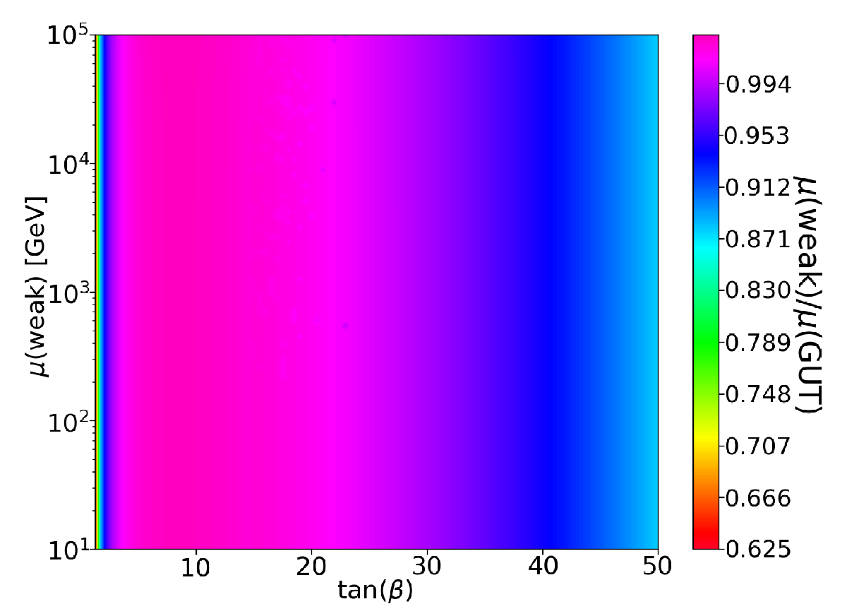
Figure 4: Ratio of $\mu/\mu_{0}$ in the $\tan\beta$ vs. $\mu(\text{weak})$ plane, where $\mu_{0}$ is the GUT-scale value of the $\mu$ parameter.

Now, in the case where all soft terms are determined in terms of $m_{3/2}$ (such as gravity-mediation, anomaly-mediation and mirage-mediation), then we expect roughly that

$$m_{Z}^{2}\simeq-2\mu^{2}+a\cdot m_{3/2}^{2}$$ (13)

and since $\mu$ hardly evolves, then $a\cdot m_{3/2}^{2}\simeq-2m_{H_{u}}^{2}(weak)$. In this case – with all correlated soft terms (which we may dub as the SUGRA1 model) – then $\Delta_{\rm BG}\sim c_{m_{3/2}^{2}}=am_{3/2}^{2}/m_{Z}^{2}\simeq max[2\mu^{2},2m_{H_{u}}^{2}(weak)]/m_{Z}^{2}$. This latter case we will find is nearly the same as $\Delta_{\rm EW}$ aside from the inclusion of the radiative corrections to the weak scale scalar potential.

In Fig. 5, we plot naturalness contours in the same parameter plane as in Fig. 3, but now assuming instead the one-soft-parameter SUGRA1 model, For SUGRA1, we have

$$m_{Z}^{2}=-2.18\mu_{0}^{2}+a\cdot m_{0}^{2}\ \ \ \text{(SUGRA1)}$$ (14)

where the constant $a$ can be determined via $a=(m_{Z}^{2}+2.18\mu_{0}^{2})/m_{0}^{2}$.

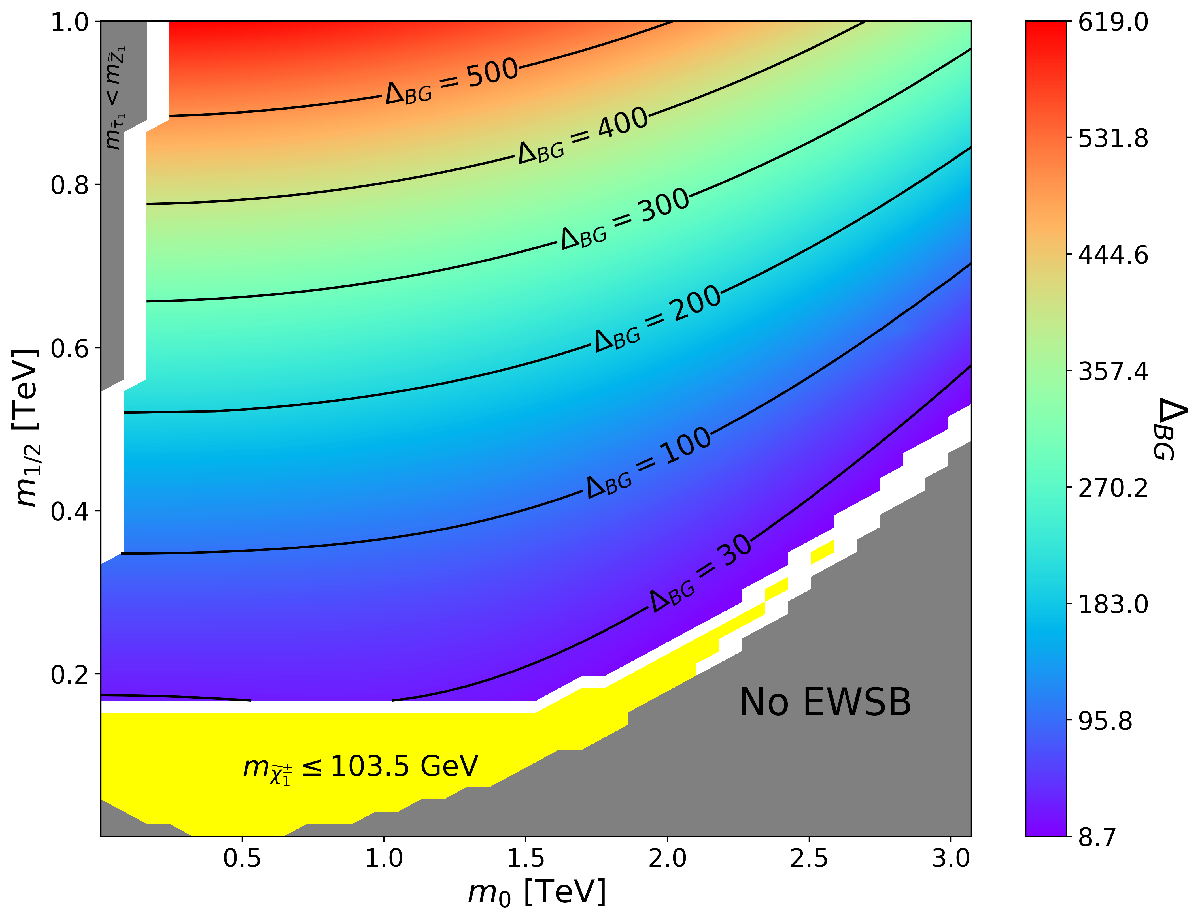
Figure 5: Plot of naturalness contours $\Delta_{BG}$ in the $m_{0}$ vs. $m_{1/2}$ plane of the one-soft-parameter SUGRA1 model with $A_{0}=0$, $\tan\beta=10$ and $\mu>0$. We use SoftSUSY to generate the spectra.

In this case, the naturalness contours roughly follow the contours of constant $\mu$ value. (The $\mu$ term all by itself has been advocated as a measure of naturalness by Chan et al.[54].) For the case of SUGRA1, the naturalness contours are very different from the case of independent high scale soft terms assumed in the mSUGRA/CMSSM model.

One may also define a SUGRA2 model. Here, we assume that since gaugino masses arise from the gauge kinetic function, this soft term is independent of the others which are determined instead by the Kähler function, but where $A_{0}$ is determined in terms of $m_{0}$ (such as $A_{0}=-2m_{0}$) so that

$$m_{Z}^{2}=-2.18\mu_{0}^{2}+3.786m_{1/2}^{2}-0.427m_{0}^{2}+1.642m_{1/2}m_{0}\ \ \ (SUGRA2).$$ (15)

Finally, SUGRA3 allows that $A_{0}$ is somehow independent from $m_{0}$ (or $m_{3/2}$) so that

$$m_{Z}^{2}=-2.18\mu_{0}^{2}+3.786m_{1/2}^{2}+0.013m_{0}^{2}+1.642m_{1/2}m_{0}+0.22A_{0}^{2}\ \ \ (SUGRA3).$$ (16)

For the three cases, we find that the $\Delta_{\rm BG}$ values are very different in the SUGRA1, SUGRA2 or SUGRA3 models just depending on which parameters are assumed to be truly independent.

In Fig. 6, we show color coded regions of $\Delta_{\rm BG}$ as computed in the $m_{0}$ vs. $m_{1/2}$ plane of the NUHM2 model where $\tan\beta=10$, $A_{0}=-1.6m_{0}$ with $\mu=200$ GeV and $m_{A}=2$ TeV. In frame a), we assume all soft terms are correlated as in Eq. 14. In this case, since $\mu$ is fixed, there is a constant value of $\Delta_{\rm BG}=21.2$ throughout the plane.

In frame b), we instead assume two independent soft parameters $m_{0}$ and $m_{1/2}$ (but with $A_{0}$ fixed in terms of $m_{0}$) so that we are in the SUGRA2 model, Eq. 15. Here, the value of $\Delta_{\rm BG}$ is vastly different from frame a), reaching up to values of $\sim 3900$ in the upper-right corner: a factor of $\sim 180$ times greater than the frame a) value. Here, the $\Delta_{\rm BG}$ finetuning is dominated by the $m_{1/2}$ value but not so much by $m_{0}$. In frame c), instead we show values of $\Delta_{\rm BG}$ assuming three independent soft parameters as in Eq. 16. In this case, with $A_{0}$ fixed as $A_{0}=-1.6m_{0}$ but nonetheless declared as independent, we see a greater dependence on $m_{0}$, so $\Delta_{\rm BG}$ increases as $m_{0}$ increases, mainly because $A_{0}$ increases with increasing $m_{0}$. Here, $\Delta_{\rm BG}$ reaches maximal values of $\sim 14500$ in the upper-right corner, a factor $\sim 680$ larger than the frame a) value!

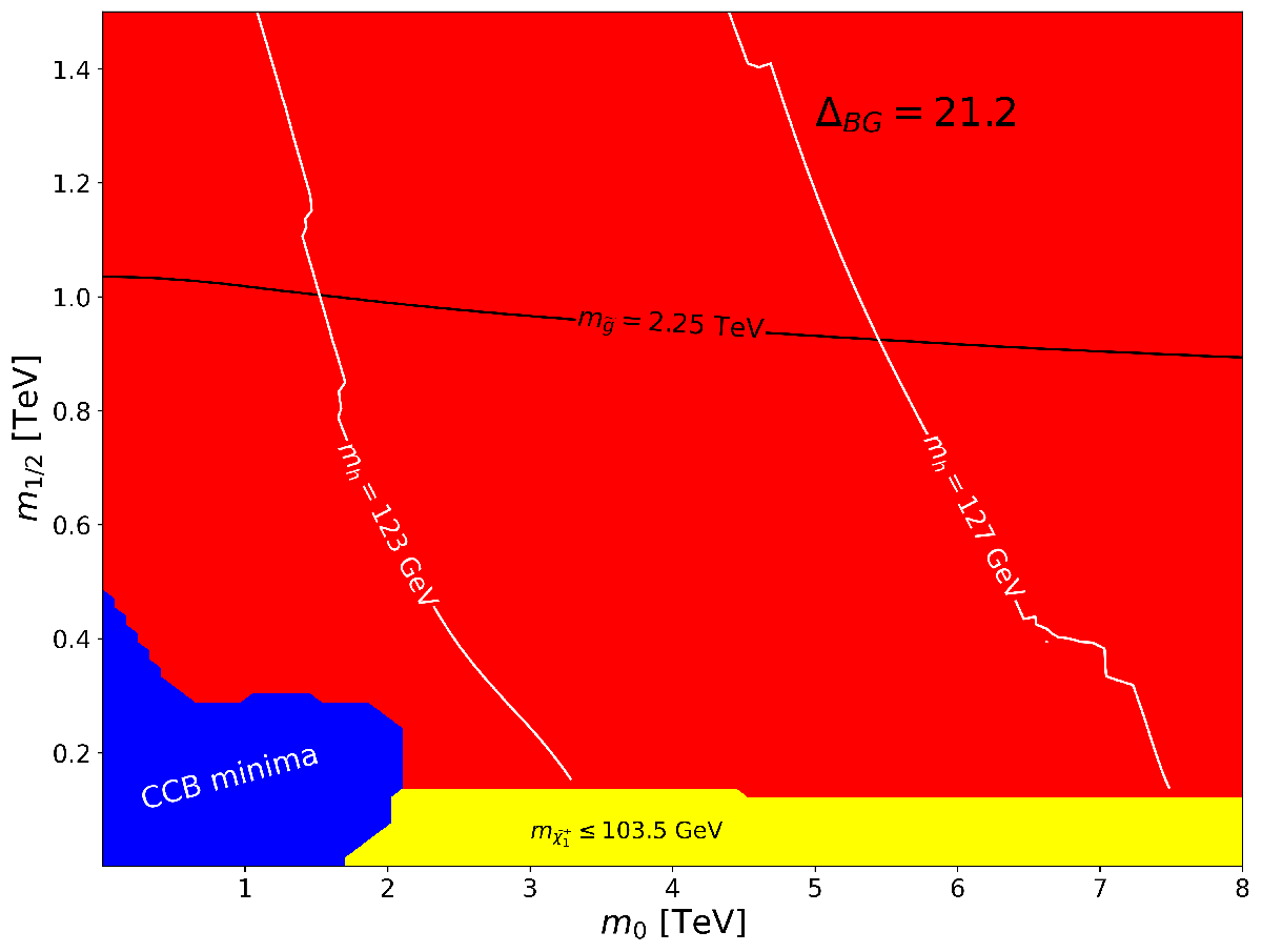
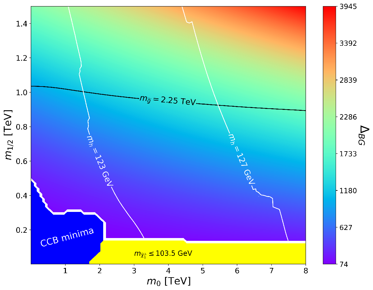
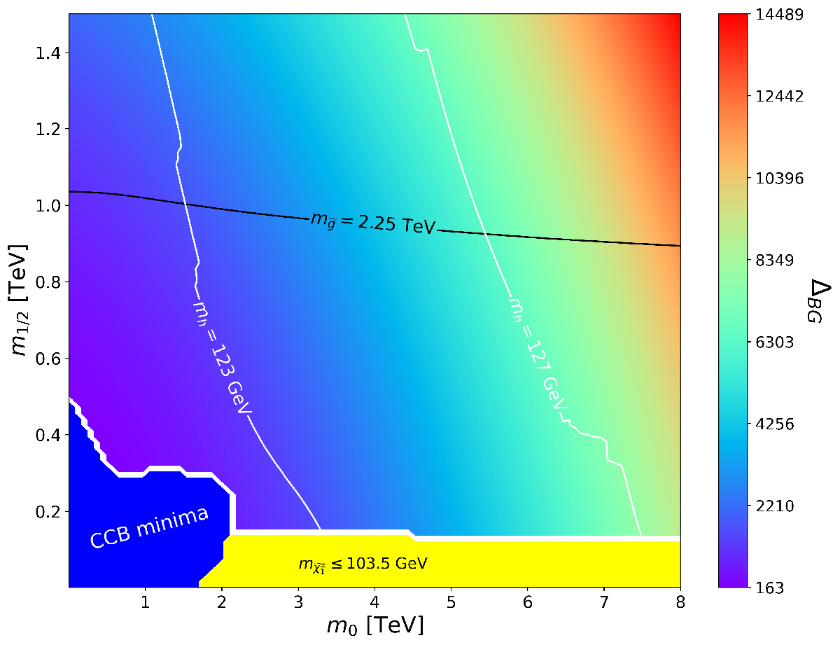
Figure 6: Plot of $\Delta_{\rm BG}$ values in the $m_{0}$ vs. $m_{1/2}$ plane for the NUHM2 model for $A_{0}=-1.6m_{0}$, $\tan\beta=10$ with $\mu=200$ GeV and $m_{A}=2$ TeV. In a), we plot $\Delta_{\rm BG}$ assuming a single independent soft parameter $m_{3/2}$ while in b) we plot $\Delta_{\rm BG}$ for assumed two independent soft parameters $m_{0}$ and $m_{1/2}$ while in c) we plot assuming all three of $m_{0}$, $m_{1/2}$ and $A_{0}$ are independent. The spectrum is calculated using SoftSUSY and the naturalness measures with DEW4SLHA.

In summary, from the discussion of this Section, we see that the measure $\Delta_{\rm BG}$ could be a legitimate finetuning measure if there could be consensus on what constitutes independent parameters of the model. The plots also illustrate the extreme model-dependence of $\Delta_{\rm BG}$, where $\Delta_{\rm BG}$ can obtain values differing by several orders of magnitude depending on which parameters $p_{i}$ are assumed fundamental or independent.

4.2 High scale finetuning

An alternative to EENZ/BG naturalness which we label as high scale finetuning (HS) emerged early on in the 21st century. It may have been intended originally as a figurative bullet point indicator to argue for sparticle masses near the weak scale[45], but later was taken more seriously[46, 49, 50, 51]. This measure seeks to apply PN to the Higgs boson mass relation (see e.g. Eq. 10 of [94])

$$m_{h}^{2}\simeq\mu^{2}+m_{H_{u}}^{2}(weak)+{\rm EW}+{\rm mixing}$$ (17)

where the EW corrections and mixings are already $\lesssim m_{h}^{2}$. The idea then is to break $m_{H_{u}}^{2}(weak)$ into $m_{H_{u}}^{2}(m_{GUT})+\delta m_{H_{u}}^{2}$ and require $\delta m_{H_{u}}^{2}\lesssim m_{h}^{2}$. The full one-loop expression for $\delta m_{H_{u}}^{2}$ may be obtained by integrating its one-loop RGE from $m_{GUT}$ to $m_{weak}$:

$$\frac{dm_{H_{u}}^{2}}{dt}=\frac{2}{16\pi^{2}}\left(-\frac{3}{5}g_{1}^{2}M_{1}^{2}-3g_{2}^{2}M_{2}^{2}+\frac{3}{10}g_{1}^{2}S+3f_{t}^{2}X_{t}\right)$$ (18)

where $t=\log Q$, $S=m_{H_{u}}^{2}-m_{H_{d}}^{2}+Tr\left[{\bf m}_{Q}^{2}-{\bf m}_{L}^{2}-2{\bf m}_{U}^{2}+{\bf m}_{D}^{2}+{\bf m}_{E}^{2}\right]$ and $X_{t}=m_{Q_{3}}^{2}+m_{D_{3}}^{2}+m_{H_{u}}^{2}+A_{t}^{2}$. In the literature[49, 50, 51], to gain a simple expression, the terms with gauge couplings are ignored and $X_{t}$ is approximated as $X_{t}\sim m_{Q_{3}}^{2}+m_{D_{3}}^{2}+A_{t}^{2}$, where $m_{Q_{3}}^{2},m_{D_{3}}^{2},$ and $A_{t}^{2}$ here are GUT-scale values. Then a single step integration leads to

$$\delta m_{H_{u}}^{2}\sim-\frac{3}{8\pi^{2}}f_{t}^{2}\left(m_{Q_{3}}^{2}+m_{U_{3}}^{2}+A_{t}^{2}\right)\log\left(\Lambda/m_{weak}\right)$$ (19)

where the high scale $\Lambda$ is usually assumed $\sim m_{GUT}$. The $\Delta_{\rm HS}$ measure famously promoted three light third generation squarks below the 500 GeV scale[50], and motivated intensive searches by the LHC collaborations to root out light top-squark signals.

In order to compare $\Delta_{\rm HS}$ more appropriately with $\Delta_{\rm BG}$ and $\Delta_{\rm EW}$, we slightly redefine $\Delta_{\rm HS}$ in terms of $m_{Z}^{2}/2$[95] where in this case we take

$$m_{Z}^{2}/2=\frac{(m_{H_{d}}^{2}(\Lambda)+\delta m_{H_{d}}^{2}+\Sigma_{d}^{d})-(m_{H_{u}}^{2}(\Lambda)+\delta m_{H_{u}}^{2}+\Sigma_{u}^{u})\tan^{2}\beta}{\tan^{2}\beta-1}-(\mu^{2}(\Lambda)+\delta\mu^{2})$$ (20)

and $\Lambda$ is some input high scale, perhaps $m_{P}$ or $m_{GUT}$. Then

$$\Delta_{\rm HS}=max|{\rm largest}\ {\rm term}\ {\rm on}\ {\rm RHS}\ {\rm of}\ {\rm Eq.}\ \ref{eq:mzsHS}|.$$ (21)

In this way, the three measures become equal in certain limiting cases.

The $\Delta_{\rm HS}$ measure is problematic on several counts

1. It violates the PN precept in that, in simplifying $\delta m_{H_{u}}^{2}$, all dependence on $m_{H_{u}}^{2}(\Lambda)$ is lost, which hides the fact that $\delta m_{H_{u}}^{2}$ is actually dependent on $m_{H_{u}}^{2}(\Lambda)$. In fact, the bigger the assumed value for $m_{H_{u}}^{2}(\Lambda)$, then the bigger is the cancelling correction $\delta m_{H_{u}}^{2}$[96]. This is shown in Fig. 7 where we show the exact two-loop value of $\delta m_{H_{u}}^{2}$ vs. $m_{H_{u}}^{2}(GUT)$, where the clear dependence of $\delta m_{H_{u}}^{2}$ on $m_{H_{u}}^{2}(GUT)$ is shown. The plot also shows that the bigger $m_{H_{u}}(GUT)$ becomes, then the more EW-natural the model becomes in that $m_{H_{u}}^{2}(weak)$ becomes comparable to $m_{Z}^{2}$ on the right-hand-side shortly before EWSB is no longer broken. The splitting up of $m_{H_{u}}^{2}(weak)$ into $m_{H_{u}}^{2}(\Lambda)+\delta m_{H_{u}}^{2}$ turns $\Delta_{\rm HS}$ into contradiction with $\Delta_{\rm BG}$, where $m_{H_{u}}^{2}(weak)$ is expanded into high scale parameters in Eq. 10 but not split into $m_{H_{u}}^{2}(\Lambda)+\delta m_{H_{u}}^{2}$. This splitting of $m_{H_{u}}^{2}(weak)$ into dependent parts destroys the cancellations needed for focus point SUSY[39, 40] which is promoted as allowing for TeV-scale top-squarks.

2. Electroweak symmetry breaking in SUSY models is accomplished by driving $m_{H_{u}}^{2}$ to negative values owing to the large top-quark Yukawa coupling $f_{t}$. Indeed, the REWSB mechanism is touted as one of the triumphs of WSS since it required $m_{t}\sim 100-200$ GeV[9] at a time when experiments seemed to indicate $m_{t}\sim 40$ GeV. By requiring $\delta m_{H_{u}}^{2}$ to be small, then often $m_{H_{u}}^{2}(weak)$ will not be large-negative enough to cause EWSB. In the context of vacua selection in the string landscape, such models without EWSB would likely not lead to inhabitable universes and would be vetoed. This can be viewed as a selection mechanism to favor models with large enough $\delta m_{H_{u}}^{2}$ such that EW symmetry is properly broken (see e.g. Fig. 3 of Ref. [97].)

3. There is also substantial ambiguity in evaluating $\Delta_{\rm HS}$. In Fig. 8 we show the value of $\delta m_{H_{u}}\equiv sign(\delta m_{H_{u}}^{2})\sqrt{|\delta m_{H_{u}}^{2}|}$ vs. $m_{H_{u}}(m_{GUT})$ for a NUHM2 benchmark point with $m_{0}=4.5$ TeV, $m_{1/2}=1$ TeV, $A_{0}=-7.2$ TeV with $\tan\beta=10$ and $m_{A}=2$ TeV. The approximate expression Eq. 19 is shown as the flat red-dashed line which of course doesn’t depend on $m_{H_{u}}^{2}(m_{GUT})$. The solid blue curve is the exact two-loop RG expression for $\delta m_{H_{u}}$ and is shown to deviate from the approximate result by well over a factor of 2 at low $m_{H_{u}}(m_{GUT})$ and only agrees with the approximation far into the excluded region where the electroweak symmetry isn’t properly broken. Alternatively, one may use the $m_{h}^{2}\simeq\mu^{2}+m_{H_{u}}^{2}+\delta m_{H_{u}}^{2}$ equation for a particular set of input parameters including $m_{H_{u}}^{2}(m_{GUT})$ (e.g. in the NUHM2 model) to compute the value of $\delta m_{H_{u}}^{2}$ and then try to finetune $m_{H_{u}}^{2}(m_{GUT})$ to enforce $m_{h}=125$ GeV. But as one tunes the value of $m_{H_{u}}^{2}(m_{GUT})$, then the value of $\delta m_{H_{u}}^{2}$ changes accordingly (as indicated by the varius dotted lines for different input $\mu$ values), so that instead of finetuning, one must adopt an iterative procedure to try and find a solution. Sometimes the solution will migrate into the noEWSB region while other times the iterations can find a viable solution.

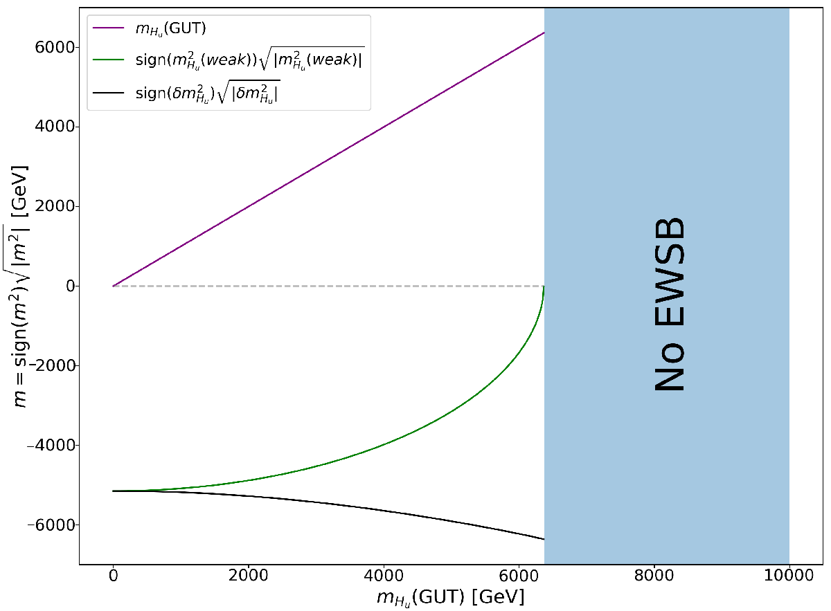
Figure 7: Plot of $sign(\delta m_{H_{u}}^{2})\cdot\sqrt{|\delta m_{H_{u}}^{2}|}$ vs. $m_{H_{u}}(GUT)$ for the NUHM2 model with $m_{0}=5$ TeV, $m_{1/2}=1.2$ TeV, $A_{0}=-1.6m_{0}$, $\tan\beta=10$ and $m_{H_{d}}=5$ TeV.

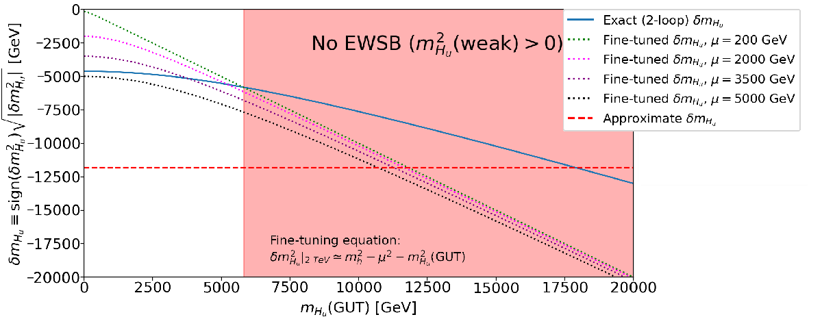
Figure 8: Plot of $sign(\delta m_{H_{u}}^{2})\cdot\sqrt{|\delta m_{H_{u}}^{2}|}$ vs. $m_{H_{u}}(GUT)$ for the NUHM2 model with $m_{0}=4.5$ TeV, $m_{1/2}=1$ TeV, $A_{0}=-7.2$ TeV and $\tan\beta=10$ with $m_{A}=2$ TeV. We show the approximate expression Eq. 18 (red-dashed curve) along with exact 2-loop expression (blue solid) along with the value gleaned from finetuning for various values of $\mu$.

4.3 Electroweak naturalness

As mentioned before, the electroweak naturalness measure $\Delta_{\rm EW}$ measures the largest contribution on the right-hand-side of Eq. 3 and compares that to $m_{Z}^{2}/2$. This is the most conservative, unavoidable measure of naturalness since it is independent of any high scale model. Even when high scale parameters are correlated in some way, those correlations are typically lost under RG running and subsequent computation of the physical sparticle mass eigenstates. The interpretation of $\Delta_{\rm EW}$ is clear: if any one of the RHS contributions to Eq. 3 is far larger than $m_{Z}^{2}/2$, then it is highly implausible (but not impossible) that some other contribution would accidentally be large, opposite-sign such that the two conspire to give an $m_{Z}$ value of just $91.2$ GeV. In this sense, natural models correspond to plausible models; models with large $\Delta_{\rm EW}$ are logically possible, but highly implausible. We’ll see later that this manifests itself as a probability, or likelihood, to emerge from scans over the string landscape.

The tree-level contributions to $\Delta_{\rm EW}$ are instructive:

• the SUSY conserving $\mu$ parameter, which sets the mass scale for the $W$, $Z$, $h$ and $higgsinos$ enters the weak scale directly. We already know that $m_{W,Z,h}\sim 100$ GeV; the higgsinos should lie within a factor of several of the measured value of the weak scale. In light of LHC constraints, the SUSY LSP is likely a higgsino-like lightest neutralino, or at worst a gaugino-higgsino admixture.

• The value of $m_{H_{u}}^{2}$, where $H_{u}$ acts as the SM Higgs doublet, should be driven to small, negative values since it also sets the mass of the $W$, $Z$ and $h$ bosons.

• The value of $m_{H_{d}}$– which sets the mass scale for the heavier Higgs bosons $A$, $H$ and $H^{\pm}$– can be much larger since its contribution to the weak scale is suppressed by a factor $\tan\beta$.

The loop-level contributions $\Sigma_{u}^{u}$ and $\Sigma_{d}^{d}$ are proportional to the individual particle/sparticle masses but since the $\Sigma_{d}^{d}$ terms are suppressed by $\tan\beta$, the $\Sigma_{u}^{u}$ terms are usually dominant. Of the $\Sigma_{u}^{u}$ terms, usually $\Sigma_{u}^{u}(\tilde{t}_{1,2})$ are largest owing to the large top-quark Yukawa coupling. Since these terms are all suppressed by loop factors, the particle/sparticle masses which enter the $\Sigma_{u}^{u}$ terms can be at the TeV or beyond scale before becoming comparable to the weak scale. Explicit expressions for the $\Sigma_{u}^{u}$ and $\Sigma_{d}^{d}$ are given in the Appendices to Ref’s [98] and [53]. The dominant terms are given by

$$\Sigma_{u}^{u}(\tilde{t}_{1,2})=\frac{3}{16\pi^{2}}F(m_{\tilde{t}_{1,2}}^{2})\left[f_{t}^{2}-g_{Z}^{2}\mp\frac{f_{t}^{2}A_{t}^{2}-8g_{Z}^{2}(\frac{1}{4}-\frac{2}{3}x_{W})\Delta_{t}}{m_{\tilde{t}_{2}}^{2}-m_{\tilde{t}_{1}}^{2}}\right]$$ (22)

where $F(m^{2})=m^{2}\left(\log\frac{m^{2}}{Q^{2}}-1\right)$ and the optimized scale choice is taken as $Q^{2}=m_{\tilde{t}_{1}}m_{\tilde{t}_{2}}$. Also, $\Delta_{t}=(m_{\tilde{t}_{L}}^{2}-m_{\tilde{t}_{R}}^{2})/2+m_{Z}^{2}\cos 2\beta(\frac{1}{4}-\frac{2}{3}x_{W})$ with $g_{Z}^{2}=(g^{2}+g^{\prime 2})/8$ and $x_{W}=\sin^{2}\theta_{W}$; in the denominator of Eq. 22, the tree-level masses should be used.

Some highlights of the $\Sigma_{u}^{u}$ terms include the following.

• For $\Delta_{\rm EW}\lesssim 30$, the top-squark contributions $\Sigma_{u}^{u}(\tilde{t}_{1,2})$ allow for top-squarks up to $m_{\tilde{t}_{1}}\lesssim 3$ TeV and $m_{\tilde{t}_{2}}\lesssim 8$ TeV. The explicit expressions contain large cancellations for large $A_{t}$ both for $\Sigma_{u}^{u}(\tilde{t}_{1})$ and $\Sigma_{u}^{u}(\tilde{t}_{2})$. The large $A_{t}$ helps to lift $m_{h}$ into the 125 GeV range since $m_{h}$ is maximal for $x_{t}\sim\sqrt{6}m_{\tilde{t}}$[10]. This is in contrast to $\Delta_{\rm BG}$ and $\Delta_{\rm HS}$ which both prefer small trilinear soft terms. In Fig. 9 we show color-coded regions of $\Delta_{\rm BG}$ in the $m_{1/2}$ vs. $A_{0}$ plane of the mSUGRA/CMSSM model for $m_{0}=5$ TeV, $\tan\beta=10$ and $\mu>0$. We also show contours of Higgs mass $m_{h}=123$ and $127$ GeV, and contours of $\Delta_{\rm EW}$ and $\Delta_{\rm HS}$. The grey region around $A_{0}\sim 0$ is the focus point region. From the plot, we see that $\Delta_{\rm HS}$ is always large, $\Delta_{\rm HS}\gtrsim 6000$, due to the large value of $m_{0}$. Meanwhile, $\Delta_{\rm BG}$ reaches as low as $\sim 1000$, also in the FP region. $\Delta_{\rm EW}$ can reach as low as 62 in between the two $\Delta_{\rm EW}=125$ contours. As expected from the mSUGRA/CMSSM model, no points allow for both low finetuning and $m_{h}\sim 125$ GeV.

• Since first/second generation Yukawa couplings are tiny, then these sparticle masses can be much larger than the third generation, with first/second generation squarks and sleptons ranging up to $30-50$ TeV. In the context of the string landscape, this leads to a quasi-degeneracy/decoupling solution to the SUSY flavor and CP problems[72].

• Gluinos affect the $\Sigma_{u}^{u}$ via RG running and directly at the two-loop level[99]. They can range up to $m_{\tilde{g}}\lesssim 6$ TeV for $\Delta_{\rm EW}\lesssim 30$, well beyond present LHC bounds[100].

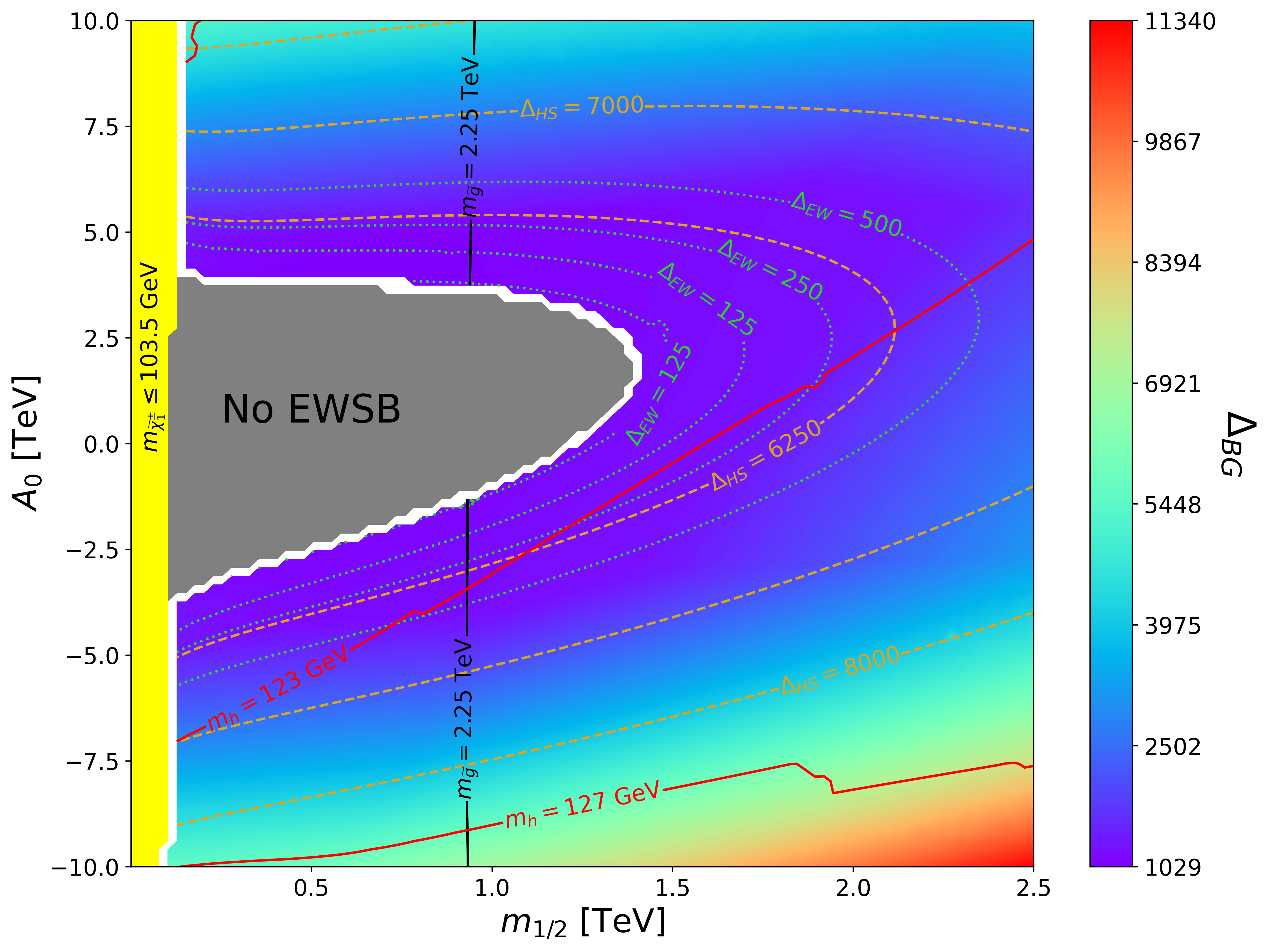
Figure 9: Plot of color-coded values of $\Delta_{\rm BG}$ in the $m_{1/2}$ vs. $A_{0}$ plane of the mSUGRA/CMSSM model for $m_{0}=5$ TeV, $\tan\beta=10$ and $\mu>0$. We also show contours of Higgs mass $m_{h}=123$ and $127$ GeV, and contours of $\Delta_{\rm EW}$ and $\Delta_{\rm HS}$.

A positive feature of $\Delta_{\rm EW}$ is its model independence (within the context of models for which the MSSM is the weak scale EFT). The amount of finetuning only depends on the weak scale spectrum which is generated, but not on how it is obtained. Thus, if one generates a certain weak scale spectrum via some high scale model, or just the pMSSM, then one gets the same value of $\Delta_{\rm EW}$. This of course isn’t true for the measures $\Delta_{\rm HS}$ or $\Delta_{\rm BG}$.

A common criticism of $\Delta_{\rm EW}$ is that it doesn’t account for high scale parameter choices and correlations. This is not exactly true as discussed earlier. The $\mu$ parameter evolves only slightly from $m_{GUT}$ to $m_{weak}$, as shown in Fig. 4. With $\mu(m_{GUT})\simeq\mu(m_{weak})$, and in the context of all soft terms correlated (as should be the case in a well specified SUSY breaking model), then $\Delta_{\rm BG}\simeq\Delta_{\rm EW}$, sans the radiative corrections $\Sigma_{u}^{u}$ and $\Sigma_{d}^{d}$. Also, if the dependent terms $m_{H_{u}}^{2}(\Lambda)$ and $\delta m_{H_{u}}^{2}$ are combined, as required by PN, then $\Delta_{\rm HS}\simeq\Delta_{\rm EW}$, sans radiative corrections. Furthermore, the specific choices of high scale parameters can lead to more or less finetuning via Eq. 3. In fact, a string landscape selection for larger soft terms often results in smaller values of $\Delta_{\rm EW}$ as compared to any selection for small or weak scale soft terms[101].

4.4 Stringy naturalness: anthropic origin of the weak scale

A fourth entry into the naturalness debate comes from Douglas[102] with regards to the string landscape: stringy naturalness, as remarked above. An advantage of stringy naturalness is that it actually provides an explanation for the magnitude of the weak scale, and not just naturalness of the weak scale. The distribution of vacua in the multiverse as a function of $m_{soft}$ is expected to be

$$dN_{vac}\sim f_{SUSY}(m_{soft})\cdot f_{EWSB}(m_{soft})dm_{soft}.$$ (23)

Douglas[102] advocates for a power-law draw to large soft terms based on the supposition that there is no favored value for SUSY breaking fields on the landscape: $f_{SUSY}\sim m_{soft}^{2n_{F}+n_{D}-1}$ where $n_{F}$ is the number of (complex-valued) $F$-breaking fields and $n_{D}$ is the number of (real-valued) $D$-breaking fields giving rise to the ultimate SUSY breaking scale. The distribution $f_{EWSB}$ is suggested as $f_{EWSB}=\Theta(30-\Delta_{\rm EW})$[103] such that the value of the weak scale in each pocket universe lies within the ABDS window[56], the so-called atomic principle. At present, SN does not admit a clear numerical measure[57].

5 Comparison of measures

From the previous discussion, it becomes clear that the various naturalness measures are defined very differently and hence we expect them to favor different regions of model parameter space. A figurative view of how the different measures compare can be gleaned from Fig. 10, which plots the evolution of the soft Higgs mass-squared parameter from $Q=m_{GUT}$ to $Q=m_{weak}$ in the NUHM2 model for $m_{0}=4.5$ TeV, $m_{1/2}=1$ TeV, $A_{0}=-1.6m_{0}$, $\tan\beta=10$ and $m_{A}=2$ TeV. The right-side brackets correspond roughly to the different naturalness measures. In NUHM2, the BG measure contains a sensitivity coefficient $c_{m_{H_{u}}^{2}}\sim 1.27|m_{H_{u}}(\Lambda)/m_{Z}|^{2}$ (or $c_{m_{H_{u}}}\sim 2.54|m_{H_{u}}(\Lambda)/m_{Z}|^{2}$ if $m_{H_{u}}(\Lambda)$ is the fundamental parameter, instead of $m_{H_{u}}^{2}(\Lambda)$). Where this coefficient is the maximal contribution to $\Delta_{\rm BG}$, then this “distance” is the approximate measure. For $\Delta_{\rm HS}\simeq\delta m_{H_{u}}^{2}/m_{Z}^{2}$, the relevant measure is instead the bracketed distance $\delta m_{H_{u}}^{2}$, and so $\Delta_{\rm HS}$ is usually (but not always) larger than $\Delta_{\rm BG}$, since in order for EW symmetry to break, $m_{H_{u}}^{2}$ must be driven to negative values. Notice then from the plot that the only way for $\delta m_{H_{u}}^{2}$ to be small is also if $m_{H_{u}}^{2}(\Lambda)$ is small: this is why $\Delta_{\rm HS}$ favors only the low $m_{0}$ region when mSUGRA/CMSSM universality with $m_{H_{u}}=m_{0}$ is required. In contrast, low values of $\Delta_{\rm EW}$ require low $m_{H_{u}}^{2}(weak)$, and so low $\Delta_{\rm EW}$ can be found for any value of $m_{H_{u}}^{2}(\Lambda)$ such that $m_{H_{u}}^{2}$ is barely driven to negative values. This is some times called criticality[104, 97], or barely broken electroweak symmetry[105]. This latter quality is favored by the string landscape where as large as possible values of $m_{H_{u}}^{2}(\Lambda)$ are statistically favored so long as $m_{Hu}^{2}$ is just barely driven to negative values[103].

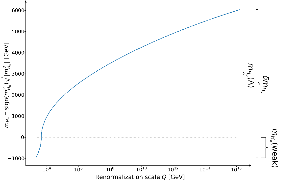
Figure 10: Evolution of the the $m_{H_{u}}^{2}$ soft SUSY breaking up-Higgs mass from $Q=m_{GUT}$ to $Q=m_{weak}$ for the NUHM2 model with $m_{0}=4.5$ TeV, $m_{1/2}=1$ TeV, $A_{0}=-1.6m_{0}$, $\tan\beta=10$ and $m_{A}=2$ TeV.

In Fig. 11a), we plot naturalness favored and unfavored regions of parameter space in the mSUGRA/CMSSM model $m_{0}$ vs. $m_{1/2}$ plane where $\tan\beta=10$, $\mu>0$ and $A_{0}=0$ (spectra generated using SoftSUSY[106]). The latter choice for $A_{0}$ is traditional in that it displays the FP region, which otherwise disappears for large $A_{0}$. However, it should be remarked here that $A_{0}=0$ is probably the least motivated value for $A_{0}$ in that in generic SUGRA models all soft terms are expected to occur of order $m_{3/2}$ and $m_{3/2}\sim m_{0}$. On the phenomenological side, small $A_{t}$ leads to a near minimum in the Higgs mass $m_{h}$ (as shown in Fig. 12) whilst $A_{t}\sim\sqrt{6}m_{0}$ leads maximal $m_{h}$ values[10]. Using high scale parameters $A_{0}$, the range of $A_{t}$ doesn’t extend to the $m_{h}$ maximal value before CCB minima are encountered in the scalar potential (which forms the endpoints of the plot). Nowadays, the mSUGRA/CMSSM FP region seems excluded by

1. too low a value of $m_{h}$[95] and

2. the LSP DM candidate is of the well-tempered[107, 108] type which is now excluded[109, 110, 111] by WIMP spin-independent direct detection experiments such as Xenon[112] and LZ[113].

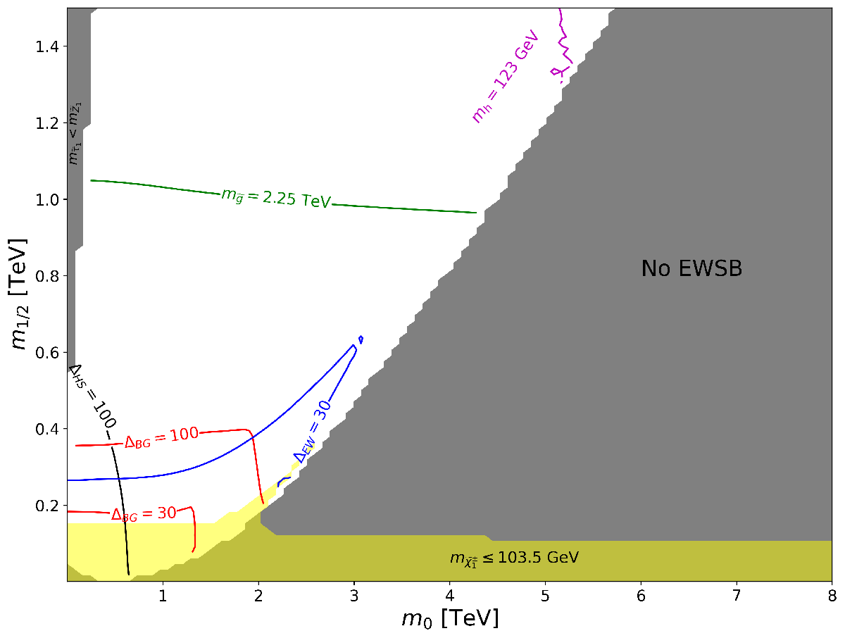
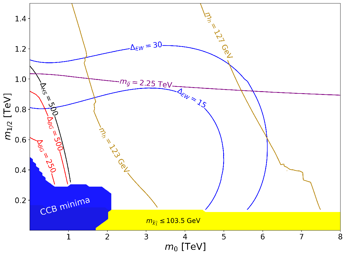
Figure 11: Plot of various naturalness contours in a) the mSUGRA/CMSSM $m_{0}$ vs. $m_{1/2}$ plane for $A_{0}=0$ and $\tan\beta=10$ and $\mu>0$. In b), we plot naturalness contours in the $m_{0}$ vs. $m_{1/2}$ plane of the NUHM2 model with $A_{0}=-1.6m_{0}$, $\tan\beta=10$, $\mu=200$ GeV and $m_{A}=2$ TeV. The spectrum is calculated using SoftSUSY and the naturalness measures with DEW4SLHA.

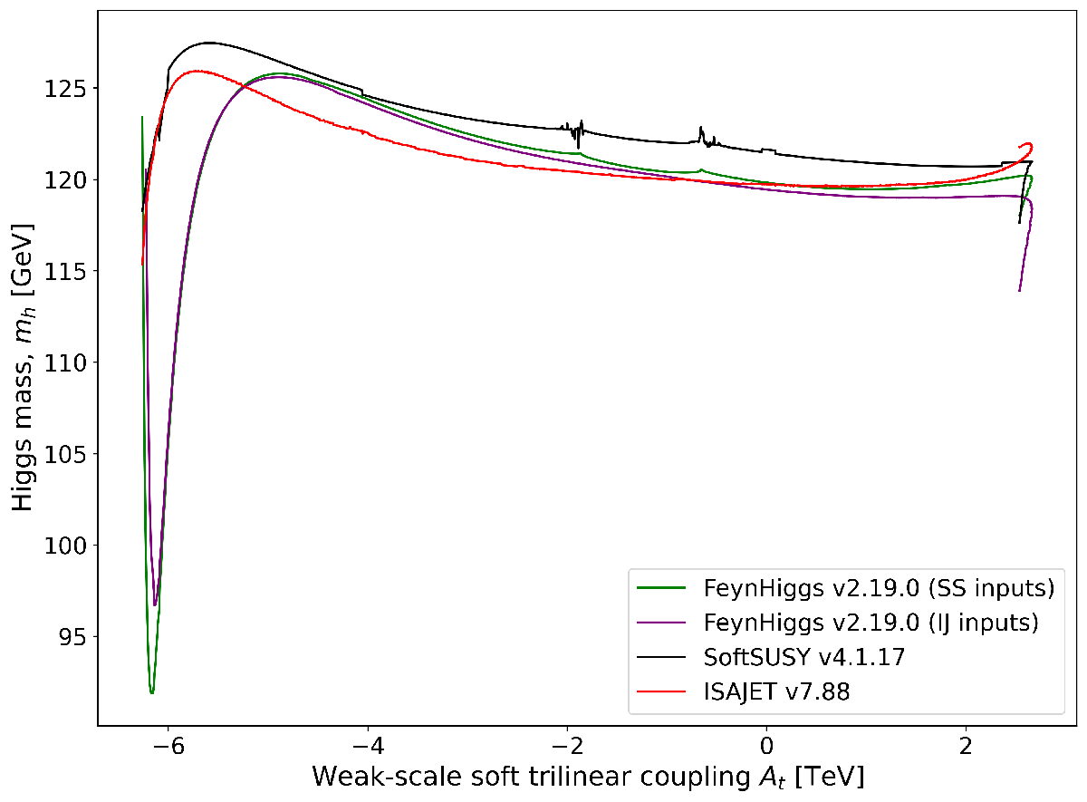
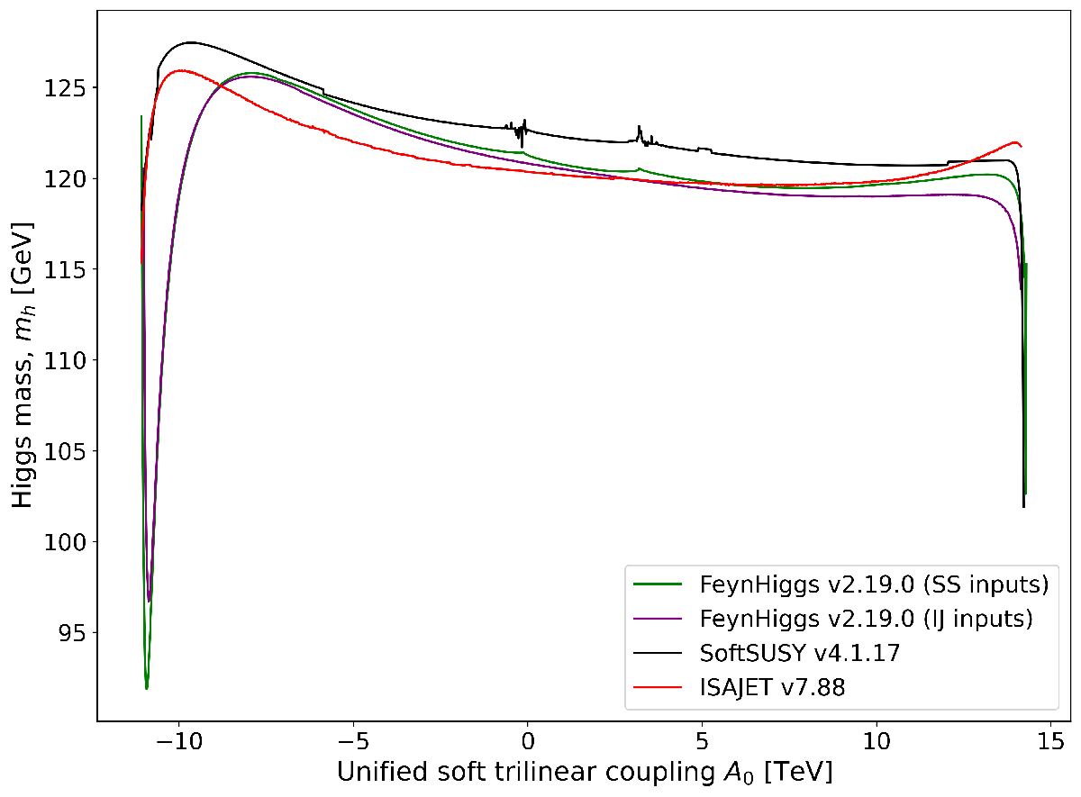
Figure 12: Computed value of $m_{h}$ vs. a) $A_{t}$ and b) $A_{0}$ in the mSUGRA/CMSSM model for $m_{0}=5$ TeV, $m_{1/2}=1.2$ TeV and $\tan\beta=10$, with $\mu>0$. We compare the results from SoftSUSY[106], FeynHiggs[114] using SoftSUSY or Isajet inputs, and Isasugra 7.88[115].

From Fig. 11a), we see the $\Delta_{\rm BG}$ contours of 30 and 100 roughly track lines of constant $\mu$ for lower $m_{0}$ values and lines of $m_{0}$ for high values[40]. Meanwhile, the contour $\Delta_{\rm EW}=30$ (denoted as blue), follows the low $\mu$ values to much larger $m_{0}$ whereupon it cuts off due to increasing top-squark contributions via the $\Sigma_{u}^{u}(\tilde{t}_{1,2})$. The conflict of these measures with $\Delta_{\rm HS}$ is apparent since $\Delta_{\rm HS}$ favors light third generation squarks which occur only at low $m_{0}$ and low $m_{1/2}$. All three measures favor the lower corner of $m_{0}$ vs. $m_{1/2}$ parameter space, and, when compared to LHC gluino mass limits ($m_{\tilde{g}}\gtrsim 2.25$ TeV as shown by the green contour), might lead one to conclude this model is excluded based on comparisons of naturalness with LHC constraints.

A very different picture emerges when one proceeds to the NUHM2 model as shown in Fig. 11b). In this case, non-universality of the Higgs soft masses (as expected in gravity-mediation) allows for low $\mu=200$ GeV throughout the parameter plane. Also, the large negative $A_{0}=-1.6m_{0}$ term allows for $m_{h}\sim 125$ GeV throughout much of the plane (as shown between the yellow contours of mass $m_{h}=123$ and $127$ GeV). The large $-A_{0}$ term helps crunch the $\Delta_{\rm HS}$ and $\Delta_{\rm BG}$ contours into the lower-left region which actually yields charge-and-color breaking scalar potential minima, which must be excluded. Meanwhile, the $\Delta_{\rm EW}$ contours balloon out to very large $m_{0}$ and $m_{1/2}$ values, with $\Delta_{\rm EW}\sim 30$ extending well beyond present LHC limits on $m_{\tilde{g}}$. While the lowest $\Delta_{\rm EW}$ values are still found in the lower-left corner of $m_{0}$ vs. $m_{1/2}$ parameter space, we note that stringy naturalness, which favors a power-law draw to large soft terms, actually favors the region beyond the LHC $m_{\tilde{g}}$ limit[57].

6 Ratios of measures for CMSSM and NUHM2 models

In this Section, we compute the ratios of various naturalness measures in the CMSSM/mSUGRA and NUHM2 models. Spectra are calculated with SoftSUSY[106] while naturalness measures are computed with DEW4SLHA[53]. The goal here is to quantify potential overestimates of finetuning in different SUSY models.

6.1 Ratios of measures for the mSUGRA/CMSSM model

6.1.1 Results in $m_{0}$ vs. $m_{1/2}$ plane

In Fig. 13, we compute the various ratios of naturalness in the mSUGRA/CMSSM model and display results in the $m_{0}$ vs. $m_{1/2}$ plane for $A_{0}=0$ and $\tan\beta=10$ (such as to include the HB/FP region. Our first results are shown in frame a) where we plot $\Delta_{\rm HS}/\Delta_{\rm BG}$. The right-side gray region has no EWSB while the left-side gray region has a stau LSP. The lower yellow region has lightest chargino below LEP2 limits of $m_{\tilde{\chi}_{1}}^{+}<103.5$ GeV. The color-coded ratios are denoted by the scale on the right-hand-side of the plot and range from 0.5 (purple) to $\sim 15$ (red).

Starting from the LHS of Fig. 13a), we see that for low $m_{0}$ then $\Delta_{\rm HS}\sim\Delta_{\rm BG}/2$. This is because $\Delta_{\rm BG}$ is typically dominated by the gluino or $M_{3}$ contribution which is then canceled by $\mu^{2}$ to maintain $m_{Z}$ at 91.2 GeV. But $\Delta_{\rm HS}$ is dominated instead by $\delta m_{H_{u}}^{2}$ which is low at low $m_{0}$. As $m_{0}$ increases, then ultimately the two measures are comparable in the color transition region while for higher $m_{0}$ values, where the FP-type cancellation kicks in, then $\Delta_{\rm HS}$ becomes much larger than $\Delta_{\rm BG}$ and reaches nearly a factor of $\sim 5-15$ at the edge of the “no EWSB” region. This plot illustrates that the $\Delta_{\rm BG}$ and $\Delta_{\rm HS}$ measures are incompatible.

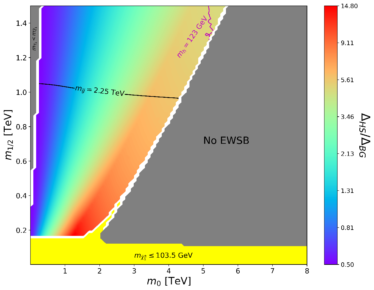
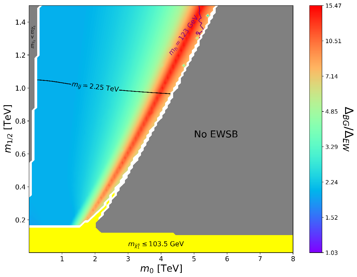
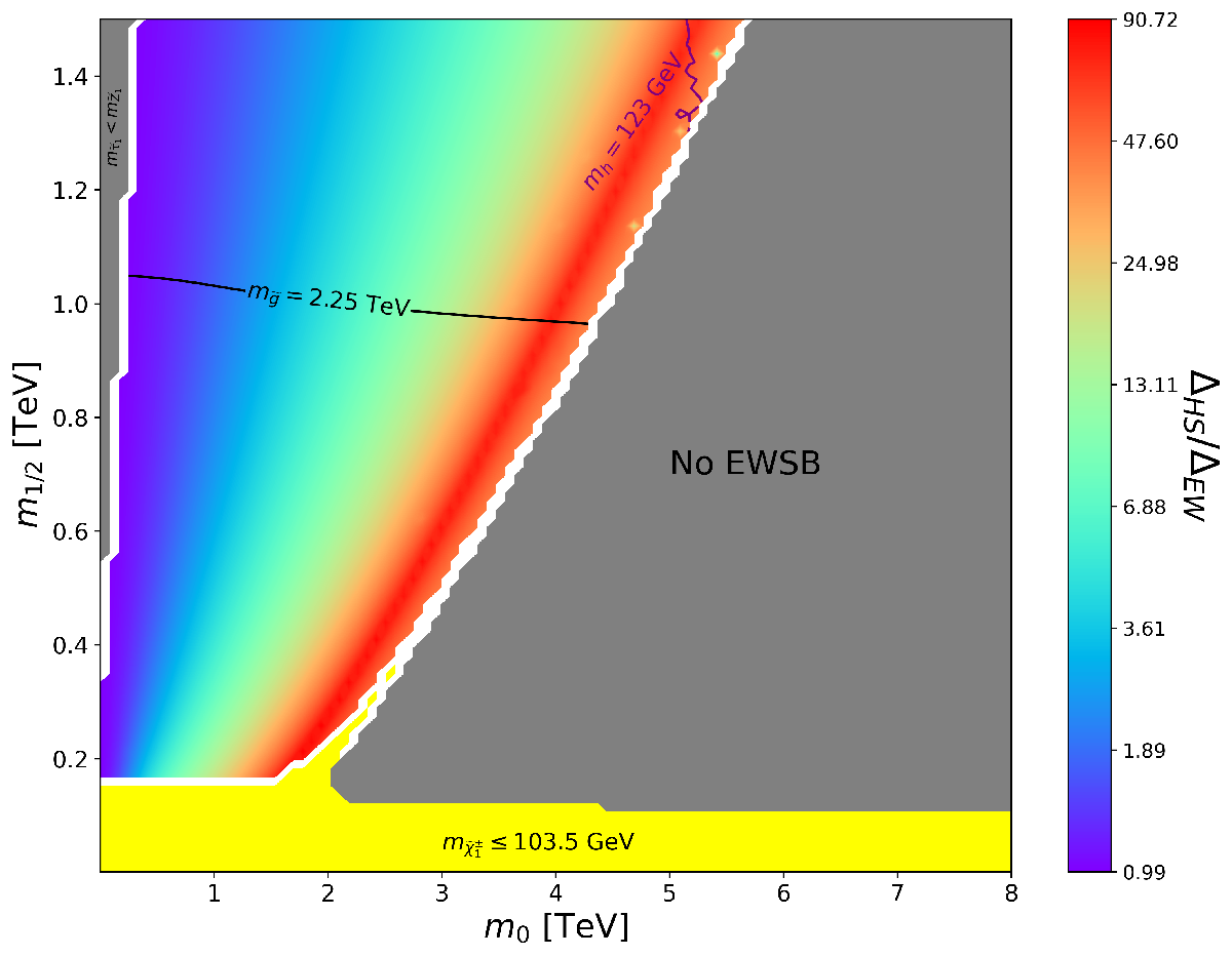
Figure 13: Plot of ratios of naturalness measures in the $m_{0}$ vs. $m_{1/2}$ plane for the CMSSM model for for $A_{0}=0$, $\tan\beta=10$ and $\mu>0$. In a), we plot $\Delta_{\rm HS}/\Delta_{\rm BG}$ while in b) we plot $\Delta_{\rm BG}/\Delta_{\rm EW}$ and in c) we plot $\Delta_{\rm HS}/\Delta_{\rm EW}$. The spectrum is calculated using SoftSUSY and the naturalness measures with DEW4SLHA.

In Fig. 13b), we plot the ratio $\Delta_{\rm BG}/\Delta_{\rm EW}$. In this case, on the left side at low $m_{0}$ the two measures are comparable, but become as large as a factor $\sim 15$ on the RHS near the edge of the no EWSB excluded region. In this region, $\Delta_{\rm BG}$ is dominated by the gluino/$M_{3}$ contribution, but in $\Delta_{\rm EW}$ this is two-loop suppressed and so $\Delta_{\rm BG}$ is much larger.

In Fig. 13c), where the ratio $\Delta_{\rm HS}/\Delta_{\rm EW}$ is plotted, we see the measures are only comparable on the extreme LHS but then differ by up to a factor of $\sim 80-100$ on the RHS in orange/red region. In this region, top-squarks are in the multi-TeV region so $\Delta_{\rm HS}$ is very large while $\Delta_{\rm EW}$ allows for multi-TeV top squarks owing to the loop factor in Eq. 22.

6.1.2 Results from scan over CMSSM parameters

Next, we attempt to pick out the maximal ratio of naturalness measures in an attempt to quantify their numerical differences. First, we scan over CMSSM parameter space

• $m_{0}:\ 0.1-15$ TeV,

• $m_{1/2}:\ 0.1-2$ TeV,

• $A_{0}:\ -2.5m_{0}$ to $+2.5m_{0}$,

• $\tan\beta:\ 3-60$

with $\mu>0$. In Fig. 14a), we show the ratio $\Delta_{\rm HS}/\Delta_{\rm BG}$ from the above scan plus a focused scan over the same parameter range but with $A_{0}=0$ so as to pick up the FP region where the ratio is expected to be largest. The green points are LHC-allowed from LHC Run 2. In this case, the ratio $\Delta_{\rm HS}/\Delta_{\rm BG}$ can be as high as 28 overall, but only as high as $\sim 10$ in the LHC-allowed region. These values are somewhat higher than the maximal ratios obtained from the plane plots.

Similarly, we show in Fig. 14b) the ratio $\Delta_{\rm BG}/\Delta_{\rm EW}$ which ranges up to 50 (20) in the overall (LHC-allowed) case. In frame it c), the ratio $\Delta_{\rm HS}/\Delta_{\rm EW}$ ranges up to $\sim 200$ for both LHC-allowed and forbidden cases.

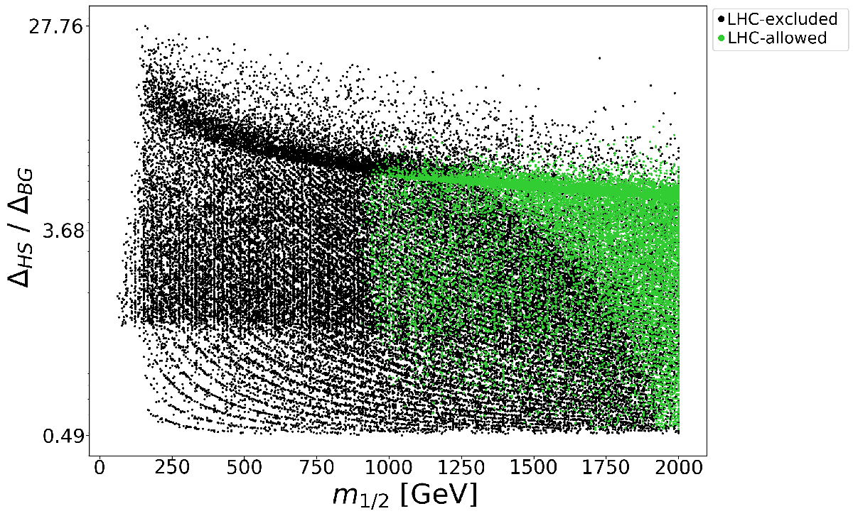
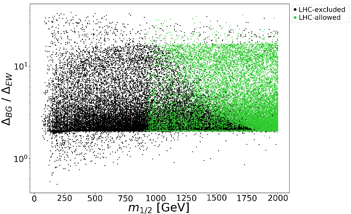
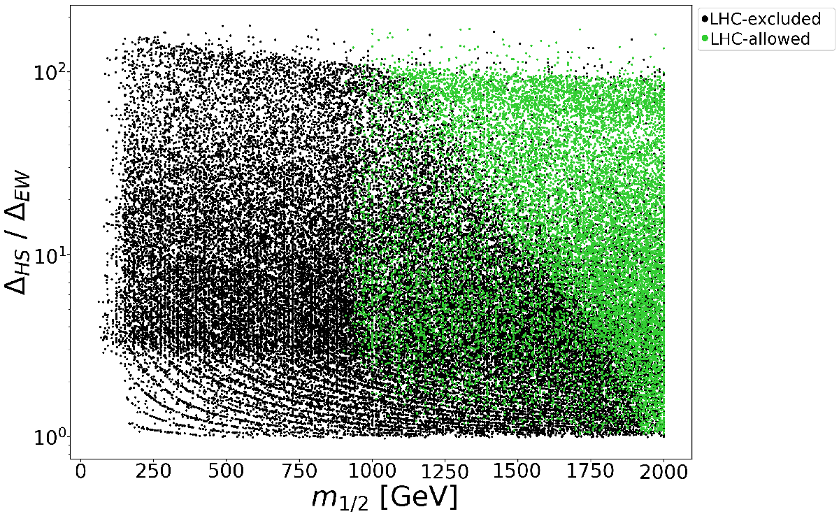
Figure 14: Plot of ratios of naturalness measures vs. $m_{1/2}$ from a scan over CMSSM model parameters. In a), we plot $\Delta_{\rm HS}$ vs. $\Delta_{\rm BG}$ for a general plus a focused scan (at $A_{0}=0$ to pick up the FP SUSY region) while in b) we plot $\Delta_{\rm BG}/\Delta_{\rm EW}$ and in c) we plot $\Delta_{\rm HS}/\Delta_{\rm EW}$. The spectrum is calculated using SoftSUSY and the naturalness measures with DEW4SLHA.

6.2 Ratios of measures for the NUHM2 model

6.2.1 Results in $m_{0}$ vs. $m_{1/2}$ plane

Next, we compute ratios of naturalness measures for the NUHM2 model. In this case, we expect much bigger differences between naturalness measures $\Delta_{\rm BG}$ and $\Delta_{\rm EW}$ since for NUHMi models, $m_{H_{u}}^{2}$ is now a free parameter, and no longer available to cancel against other oppositely signed sfermion contributions in Eq. 10. In particular, the FP cancellation between Higgs and third generation sfermion terms in Eq. 10 is destroyed when one assumes that $m_{H_{u}}^{2}$ is a free parameter. Furthermore, by adopting natural values of $\mu\sim m_{weak}$, then this contribution to $\Delta_{\rm EW}$ is suppressed and the dominant contribution instead frequently comes from the (loop-suppressed) $\Sigma_{u}^{u}(\tilde{t}_{1,2})$ terms.

In Fig. 15a), we show color-coded ratios $\Delta_{\rm HS}/\Delta_{\rm BG}$ in the $m_{0}$ vs. $m_{1/2}$ plane of the NUHM2 model with $A_{0}=-1.6m_{0}$, $\tan\beta=10$, $\mu=200$ GeV and $m_{A}=2$ TeV. The lower-left blue shaded region has CCB minima in the scalar potential owing in part to the large $A_{0}$ term. The spectra is generated using SoftSUSY. The gold contours denote Higgs mass $m_{h}=123$ GeV (left) and $m_{h}=127$ GeV (right), while the purple contour near $m_{1/2}\sim 1$ TeV denotes the LHC $m_{\tilde{g}}=2.25$ TeV limit. On the green-shaded extreme left side of the plot, $\Delta_{\rm BG}$ becomes larger than $\Delta_{\rm HS}$ by a factor $\sim 2$. For the bulk of the plot range (red- and orange- shaded regions), then $\Delta_{\rm HS}\sim(0.75-0.85)\Delta_{\rm BG}$.

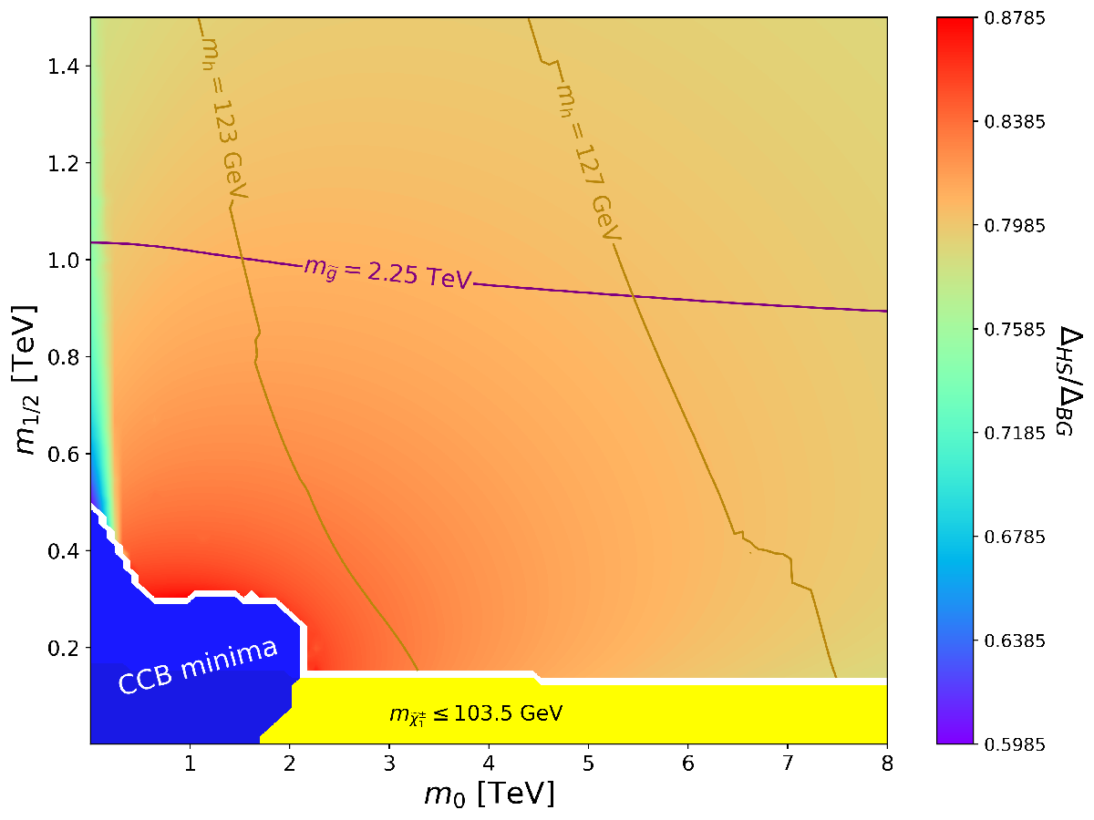
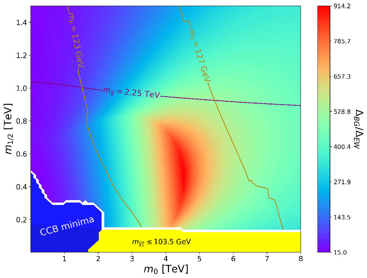
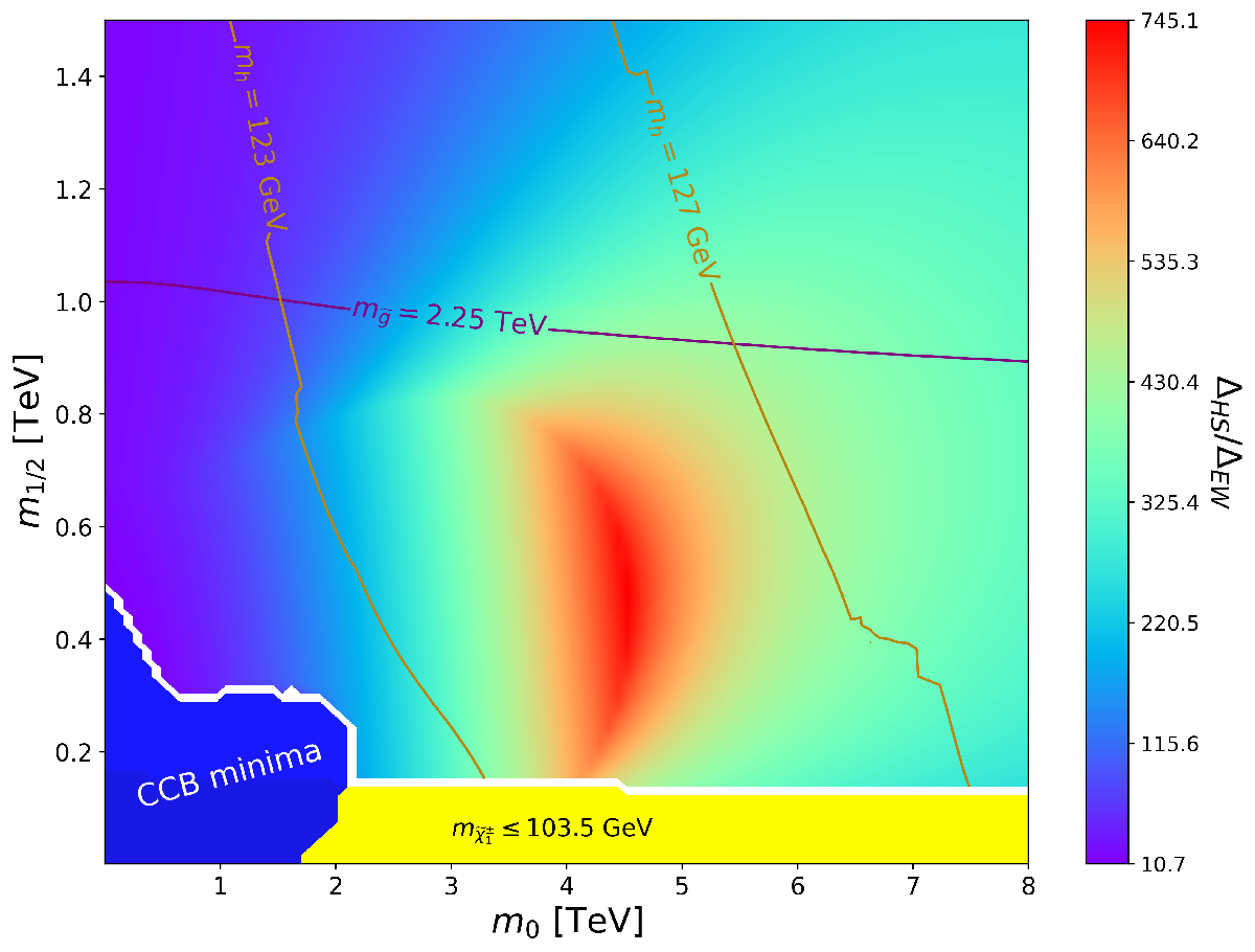
Figure 15: Plot of ratios of naturalness measures in the $m_{0}$ vs. $m_{1/2}$ plane for the NUHM2 model for $A_{0}=-1.6m_{0}$, $\tan\beta=10$ and $\mu=200$ GeV and $m_{A}=2$ TeV. In a), we plot $\Delta_{BG}/\Delta_{\rm HS}$ while in b) we plot $\Delta_{BG}/\Delta_{\rm EW}$ and in c) we plot $\Delta_{\rm HS}/\Delta_{\rm EW}$. The spectrum is calculated using SoftSUSY and the naturalness measures with DEW4SLHA.

In Fig. 15b), we show the ratio $\Delta_{\rm BG}/\Delta_{\rm EW}$ in the same plane as frame a). In the red-shaded region below the LHC gluino mass limit, we see that $\Delta_{\rm BG}/\Delta_{\rm EW}\sim 900$, a gross disparity between measures. Here, we have utilized $m_{H_{u}}$ as the fundamental parameter in place of $m_{H_{u}}^{2}$ for numerical stability purposes–the difference is only a factor of two in the derivative. In this region, $\Delta_{\rm BG}$ is dominated by the $|-1.27\cdot 2m_{H_{u}}^{2}|/(m_{Z}^{2}/2)$ term in Eq. 10 which can be $\sim 11000$ whilst the $\Delta_{\rm EW}$ measure is dominated by $\Sigma_{u}^{u}(\tilde{t}_{1,2})$ which yields $\Delta_{\rm EW}\sim 10-20$ (very natural). Throughout the NUHM2 plane, one can be brought to very different conclusions regarding the naturalness of the NUHM2 model parameter space depending on which measure one adopts! For the bulk of parameter space above the LHC gluino bound, then one finds $\Delta_{\rm BG}\sim(50-400)\Delta_{\rm EW}$.

In Fig. 15c), we show the ratio $\Delta_{\rm HS}/\Delta_{\rm EW}$. In this case, the red-shaded region shows that $\Delta_{\rm HS}\sim 700\Delta_{\rm EW}$. Again, one is led to very different conclusions on the naturalness of the model depending on which measure one chooses. In this case, in the LHC-allowed region then $\Delta_{\rm HS}\sim(50-400)\Delta_{\rm EW}$.

6.2.2 Results from scan over NUHM2 parameters

Here, we scan over NUHM2 parameter space:

• $m_{0}:\ 0.1-15$ TeV,

• $m_{1/2}:\ 0.1-2$ TeV,

• $A_{0}:\ -2.5m_{0}$ to $+2.5m_{0}$,

• $\tan\beta:\ 3-60$

• $\mu:\ 0.1-1$ TeV and

• $m_{A}:\ 0.3-8$ TeV.

From Fig. 16a), we see the ratio $\Delta_{\rm HS}/\Delta_{\rm BG}$ ranges from $\sim 0.1-1.5$ over the parameter space scanned: the two measures are rather close much of the time in this case, but sometimes $\Delta_{\rm BG}$ can become a factor of $\sim 10$ larger than $\Delta_{\rm HS}$. In Fig. 16b), instead we plot the $\Delta_{\rm BG}/\Delta_{\rm EW}$ ratio. While the bulk of parameter points have ratio between $\sim 1-250$, some few points can range up to $500-1000$. Similar results are obtained for Fig. 16c) where we plot $\Delta_{\rm HS}/\Delta_{\rm EW}$ and find ratios ranging again up to over 1000.

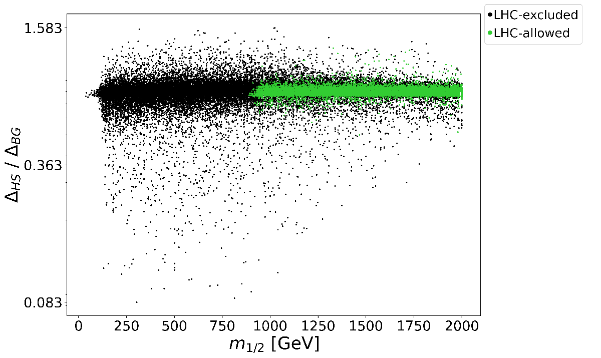
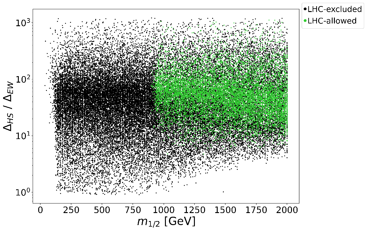
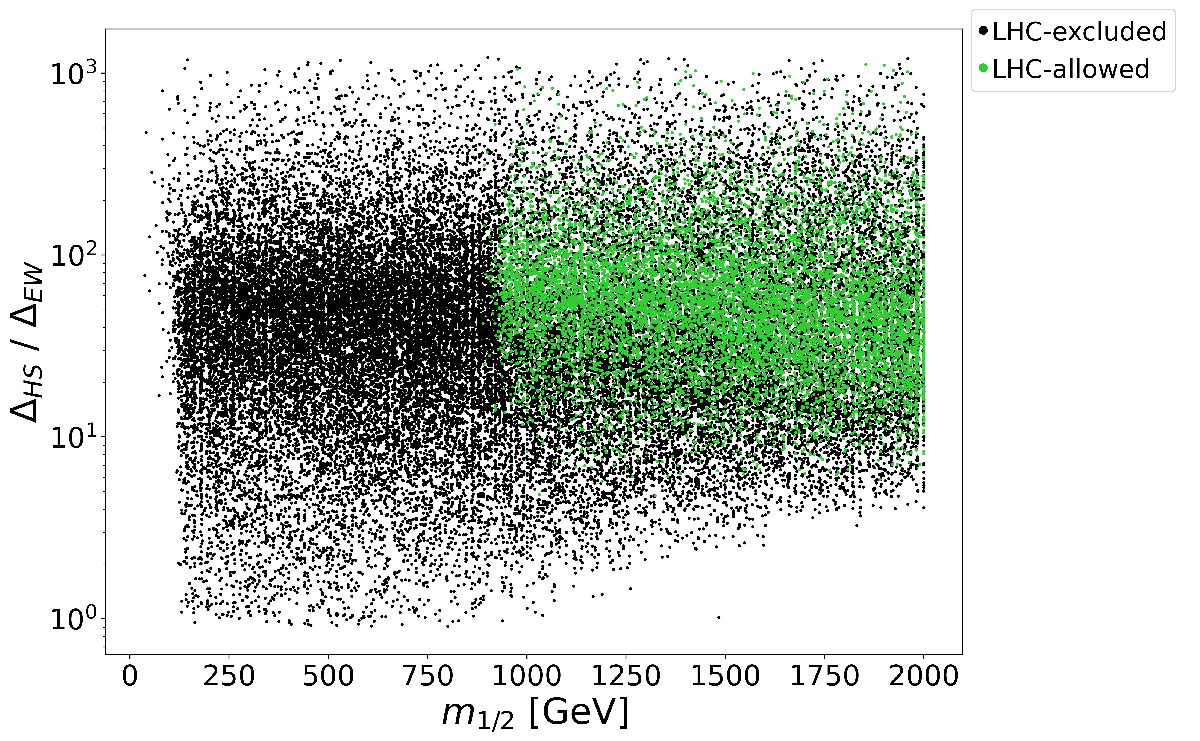
Figure 16: Plot of ratios of naturalness measures vs. $m_{1/2}$ from a scan over NUHM2 model parameters. In a), we plot $\Delta_{\rm HS}/\Delta_{\rm BG}$ while in b) we plot $\Delta_{\rm BG}/\Delta_{\rm EW}$ and in c) we plot $\Delta_{\rm HS}/\Delta_{\rm EW}$. The spectrum is calculated using SoftSUSY and the naturalness measures with DEW4SLHA.

7 Natural generalized anomaly-mediation (nAMSB)

Anomaly-mediated SUSY breaking (AMSB) models[73, 74] are good examples of models where the soft terms are all correlated and determined by a single parameter, the gravitino mass $m_{3/2}$. AMSB models assume a sequestering between the hidden and visible sector fields such that gravity-mediated soft terms are suppressed; in such a case, the loop-induced AMSB soft terms, which depend on the beta functions and anomalous dimensions of the low energy theory (assumed to be the MSSM) are dominant, and independent of higher energy physics. At first glance, AMSB SUSY models would seem ruled out since the AMSB soft terms give rise to tachyonic sleptons. In the original Randall-Sundrum paper, it is conjectured that additional bulk soft terms may also be present which can solve the tachyonic slepton mass problem.

In the so-called minimal AMSB (mAMSB) model, a universal bulk sfermion mass $m_{0}$ is also assumed so that the parameter space of mAMSB is given by

$$m_{0},\ m_{3/2},\ \tan\beta,\ sign(\mu)\ \ \ (mAMSB).$$ (24)

Here, the magnitude of a bilinear soft $B$ term is traded for the parameter $\tan\beta$ and $|\mu|$ is determined from the EW minimization condition. Famously, the wino-like neutralino turns out to be the LSP. At present, in light of LHC sparticle and Higgs mass constraints and direct/indirect wino dark matter constraints, mAMSB seems ruled out[116, 117, 109]. The small AMSB $A_{t}$ terms lead to $m_{h}\ll 125$ GeV unless sparticle masses $\sim 10-100$ TeV (highly unnatural) sparticle are assumed[118, 119] and the DM constraints are evaded.

However, in Ref. [75] some minor fixes were proposed which lead to generalized AMSB models (gAMSB) which allow for naturalness (nAMSB with $\Delta_{\rm EW}\lesssim 30$) and with $m_{h}\sim 125$ GeV. The fixes are:

1. non-universal scalar bulk masses $m_{H_{u}}\neq m_{H_{d}}\neq m_{0}$ and

2. bulk-induced $A_{0}$ terms.

3. a further option is independent bulk terms for each sfermion generation $m_{0}(i)$ with $i=1-3$.

As in NUHMi models, the non-universal bulk Higgs soft terms can be traded for $\mu$ and $m_{A}$ via scalar potential minimization conditions and the bulk $A$ terms can be chosen to dial up $m_{h}\sim 125$ GeV. Thus, the generalized AMSB parameter space is given by

$$m_{0}(i),\ m_{3/2},\ A_{0},\ \tan\beta,\ \mu\ \ {\rm and}\ \ m_{A}\ \ \ (gAMSB).$$ (25)

For natural values of $\mu\sim 100-350$ GeV, then in nAMSB the LSP is instead (usually) higgsino-like, although the wino is still the lightest of the gauginos. The gAMSB model is what one may expect in models of charged SUSY breaking, where the hidden sector SUSY breaking field $S$ contains some hidden sector charge[120]. In this case, then usual gravity-mediated gaugino masses are forbidden since the gauge kinetic function is holomorphic. But sfermion masses and $A$-terms, which depend instead on the Kähler potential, are allowed to obtain gravity-mediated soft terms. The naturalness measure $\Delta_{\rm BG}$ is harder to interpret in the AMSB case since $m_{3/2}$ plays a more fundamental role than the ad-hoc soft terms. Also, $\Delta_{\rm HS}$ is problematic in that the purely AMSB soft terms are famously scale independent, so there is no prescription for which $\Lambda$ should be used in Eq. 19. Alternatively, there is no ambiguity in the $\Delta_{\rm EW}$ measure, so we proceed to exhibit its value.

In Fig. 17, we plot color-coded regions of naturalness measure $\Delta_{\rm EW}$ in the $m_{0}$ vs. $m_{3/2}$ plane for a) the mAMSB model and b) for the nAMSB model. For both cases, we take $\tan\beta=10$ and $\mu>0$. For the nAMSB model, we also take $\mu=200$ GeV and $m_{A}=2$ TeV and $A_{0}=m_{0}$. In the case of frame a) for mAMSB, the Higgs mass $m_{h}$ is less then 123 GeV throughout the entire plane shown (and we do show a contour of $m_{h}=120$ GeV via the dotted curve). The minimal value of $\Delta_{\rm EW}$ is $\sim 25$ in the purple focus point region in the LHC-excluded zone, but $\Delta_{\rm EW}$ can range as high as over 2000 in the upper-left region.

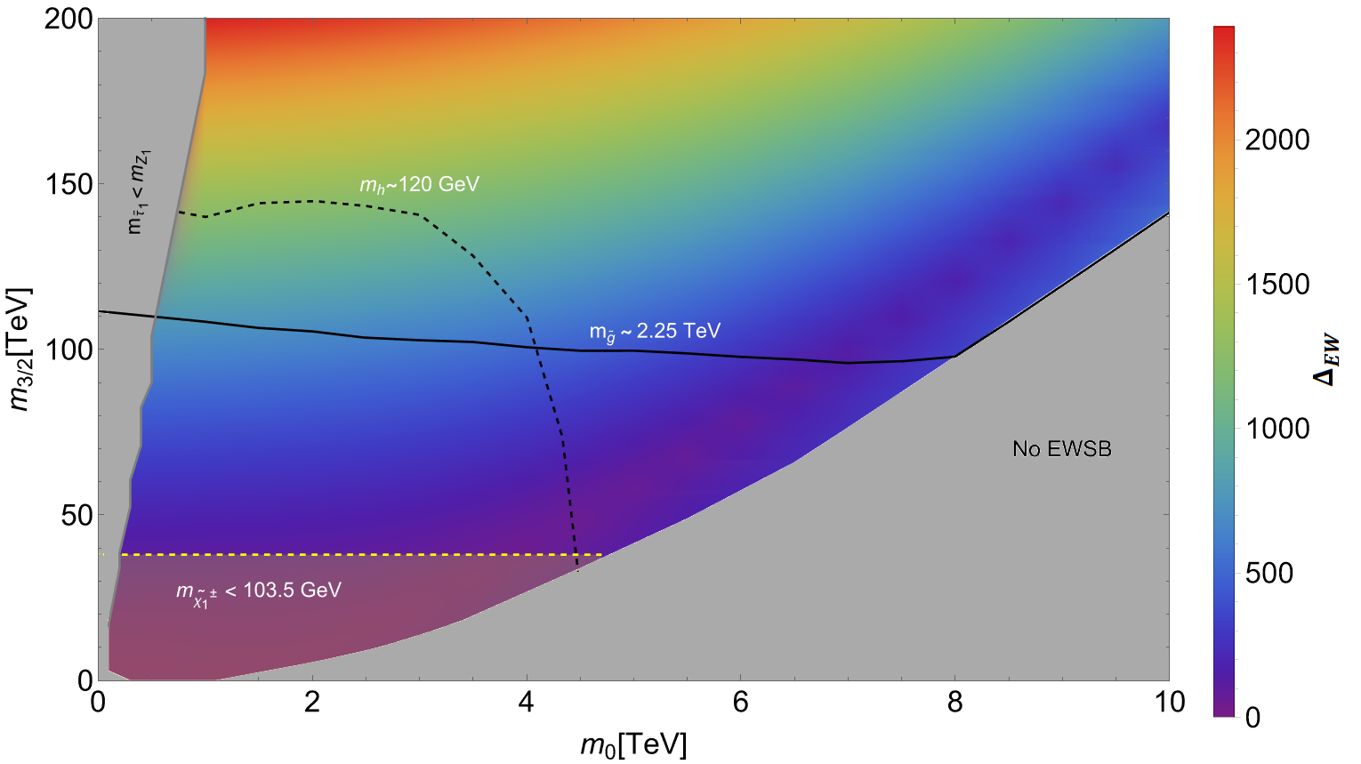
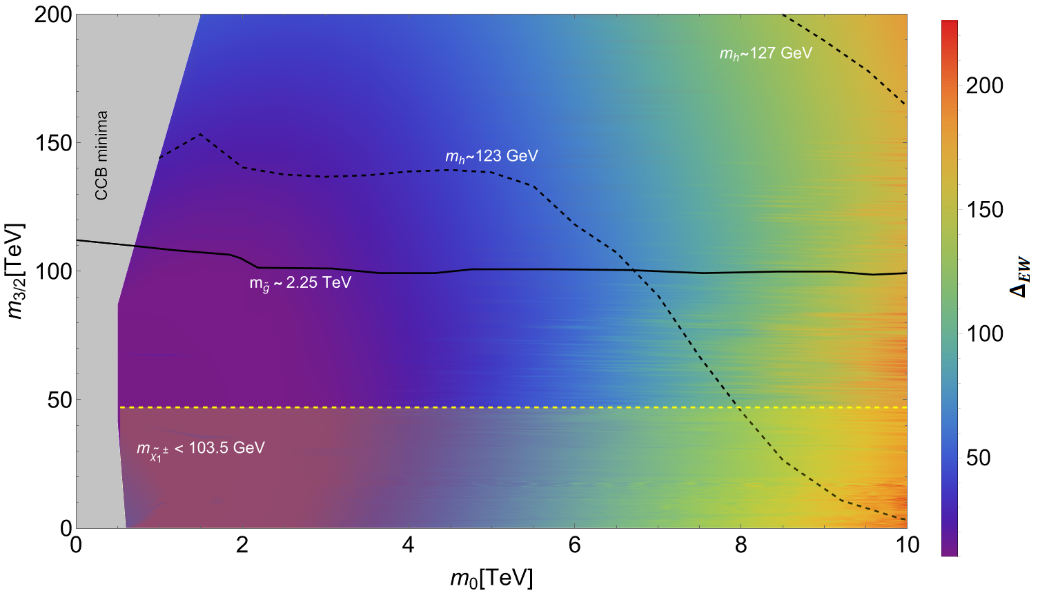
Figure 17: Plot of naturalness measure $\Delta_{\rm EW}$ in the $m_{0}$ vs. $m_{3/2}$ plane of a) the mAMSB model and b) the nAMSB model for $\tan\beta=10$. For nAMSB, we also require $\mu=200$ GeV and $m_{A}=2$ TeV. The spectrum is calculated using Isasugra.

In contrast, for frame b), we see that a large portion of the plane shown has $m_{h}\sim 123-127$ GeV. In addition, $\Delta_{\rm EW}$ can range as low as $\sim 15$ in the lower-left region, although this is excluded by LHC. In the LHC-allowed region, above the $m_{\tilde{g}}=2.25$ TeV contour, then $\Delta_{\rm EW}$ can be as low as $\sim 20$. Note that the range of color-coded $\Delta_{\rm EW}$ values is much smaller in frame b) than in a): in b), $\Delta_{\rm EW}$ ranges as high as $\sim 150$ while in a) it can range beyond 2000.

8 Natural general mirage mediation (nGMM)

While the AMSB models may seem contrived owing to the requirement of sequestering and ad hoc bulk soft terms, a perhaps more realistic alternative is mirage mediation (MM) models where gravity-mediated and anomaly-mediated soft terms are comparable. This class of models is expected to arise from IIB string compactification on an orientifold with moduli stabilization as in KKLT[121]: the dilaton $S$ and complex structure moduli $U^{\beta}$ are stabilized by fluxes and the Kähler moduli $T^{\alpha}$ are stabilized by non-perturbative effects such as gaugino condensation or instantons. While the $S$ and $U^{\beta}$ moduli are expected to gain Kaluza-Klein (KK) scale masses, the $T^{\alpha}$ moduli can be much lighter. Moduli stabilization leads to supersymmetric AdS vacua, but uplifting of the scalar potential via addition of, for instance, an anti D3 brane at the tip of a Klebanov-Strassler throat can lead to metastable deSitter vacua. A scale of hierarchies $m_{T}\sim 4\pi^{2}m_{3/2}\sim 4\pi^{2}m_{soft}$ is expected to ensue, leading to comparable moduli- and AMSB-contributions to soft masses.

The original KKLT picture assumed a single Kähler modulus $T$ and a simple uplift procedure. Within the MM model, the soft supersymmetry breaking (SSB) gaugino mass parameters, trilinear SSB parameters and sfermion mass parameters, all renormalized just below the unification scale (taken to be $Q=m_{\rm GUT}$), are found to be[76],

$$M_{a} = M_{s}\left(l_{a}\alpha+b_{a}g_{a}^{2}\right),$$ (26)

$$A_{ijk} = M_{s}\left(-a_{ijk}\alpha+\gamma_{i}+\gamma_{j}+\gamma_{k}\right),$$ (27)

$$m_{i}^{2} = M_{s}^{2}\left(c_{i}\alpha^{2}+4\alpha\xi_{i}-\dot{\gamma}_{i}\right),$$ (28)

where $M_{s}\equiv\frac{m_{3/2}}{16\pi^{2}}$, $b_{a}$ are the gauge $\beta$ function coefficients for gauge group $a$ and $g_{a}$ are the corresponding gauge couplings. The coefficients that appear in (26)–(28) are given by $c_{i}=1-n_{i}$, $a_{ijk}=3-n_{i}-n_{j}-n_{k}$ and $\xi_{i}=\sum_{j,k}a_{ijk}{y_{ijk}^{2}\over 4}-\sum_{a}l_{a}g_{a}^{2}C_{2}^{a}(f_{i}).$ Finally, $y_{ijk}$ are the superpotential Yukawa couplings, $C_{2}^{a}$ is the quadratic Casimir for the a^th gauge group corresponding to the representation to which the sfermion $\tilde{f}_{i}$ belongs, $\gamma_{i}$ is the anomalous dimension and $\dot{\gamma}_{i}=8\pi^{2}\frac{\partial\gamma_{i}}{\partial\log\mu}$. Expressions for the last two quantities involving the anomalous dimensions can be found in the Appendices of Ref’s. [122, 123]. The quantity $l_{a}$ is the power of the modulus field entering the gauge kinetic function. The $n_{i}$ are modular weights which take on discrete values in the original construction based on the brane locations of the matter superfields[76].

The MM model is then specified by the parameters

$$\ m_{3/2},\ \alpha,\ \tan\beta,\ sign(\mu),\ n_{i},\ l_{a}.$$ (29)

The mass scale for the SSB parameters is dictated by the gravitino mass $m_{3/2}$. The phenomenological parameter $\alpha$, which could be of either sign, determines the relative contributions of anomaly mediation and gravity mediation to the soft terms, and is expected to be $|\alpha|\sim{\cal O}(1)$. Grand unification implies matter particles within the same GUT multiplet have common modular weights, and that the $l_{a}$ are universal. We will assume here that all $l_{a}=1$ and, for simplicity, there is a common modular weight for all matter scalars $c_{m}$ but we will allow for different modular weights $c_{H_{u}}$ and $c_{H_{d}}$ for each of the two Higgs doublets of the MSSM. Such choices for the scalar field modular weights are motivated for instance by $SO(10)$ SUSY GUT models where the MSSM Higgs doublets may live in different ${\bf 10}$-dimensional Higgs reps.

For a variety of discrete parameter choices $n_{i}$, the various MM models have all been found to be unnatural when the Higgs mass $m_{h}$ is restricted to be $m_{h}:123-127$ GeV. However, in Ref. [77], it was suggested that to allow for more realistic compactification schemes (wherein the Kähler moduli may number in the hundreds instead of just one) and for more diverse uplifting mechanisms, then the discrete valued parameter choices may be generalized to continuous ones. This transition to generalized MM models (GMM) then allows for natural models with $m_{h}\sim 125$ GeV. The parameter space of GMM is given by

$$\alpha,\ m_{3/2},\ c_{m},\ c_{m3},\ a_{3},\ c_{H_{u}},\ c_{H_{d}},\ \tan\beta\ \ \ \ (GMM),$$ (30)

where $a_{3}$ is short for $a_{Q_{3}H_{u}U_{3}}$ (appearing in Eq. 27) and $c_{m}$, $c_{m3}$, $c_{H_{u}}$ and $c_{H_{d}}$ arise in Eq. 28. Here, we adopt an independent value $c_{m}$ for the first two matter-scalar generations whilst the parameter $c_{m3}$ applies to third generation matter scalars. The independent values of $c_{H_{u}}$ and $c_{H_{d}}$, which set the moduli-mediated contribution to the soft Higgs mass-squared soft terms, may conveniently be traded for weak scale values of $\mu$ and $m_{A}$ as is done in the two-parameter non-universal Higgs model (NUHM2)[67]:

$$\alpha,\ m_{3/2},\ c_{m},\ c_{m3},\ a_{3},\ \tan\beta,\mu,\ m_{A}\ \ \ (GMM^{\prime}).$$ (31)

This procedure allows for more direct exploration of stringy natural SUSY parameter space where most landscape solutions require $\mu\sim 100-300$ GeV in anthropically-allowed pocket universes[124].

Thus, our final formulae for the soft terms are given by

$$M_{a} = \left(\alpha+b_{a}g_{a}^{2}\right)m_{3/2}/16\pi^{2},$$ (32)

$$A_{\tau} = \left(-a_{3}\alpha+\gamma_{L_{3}}+\gamma_{H_{d}}+\gamma_{E_{3}}\right)m_{3/2}/16\pi^{2},$$ (33)

$$A_{b} = \left(-a_{3}\alpha+\gamma_{Q_{3}}+\gamma_{H_{d}}+\gamma_{D_{3}}\right)m_{3/2}/16\pi^{2},$$ (34)

$$A_{t} = \left(-a_{3}\alpha+\gamma_{Q_{3}}+\gamma_{H_{u}}+\gamma_{U_{3}}\right)m_{3/2}/16\pi^{2},$$ (35)

$$m_{i}^{2}(1,2) = \left(c_{m}\alpha^{2}+4\alpha\xi_{i}-\dot{\gamma}_{i}\right)(m_{3/2}/16\pi^{2})^{2},$$ (36)

$$m_{j}^{2}(3) = \left(c_{m3}\alpha^{2}+4\alpha\xi_{j}-\dot{\gamma}_{j}\right)(m_{3/2}/16\pi^{2})^{2},$$ (37)

$$m_{H_{u}}^{2} = \left(c_{H_{u}}\alpha^{2}+4\alpha\xi_{H_{u}}-\dot{\gamma}_{H_{u}}\right)(m_{3/2}/16\pi^{2})^{2},$$ (38)

$$m_{H_{d}}^{2} = \left(c_{H_{d}}\alpha^{2}+4\alpha\xi_{H_{d}}-\dot{\gamma}_{H_{d}}\right)(m_{3/2}/16\pi^{2})^{2},$$ (39)

where, for a given value of $\alpha$ and $m_{3/2}$, the values of $c_{H_{u}}$ and $c_{H_{d}}$ are adjusted so as to fulfill the input values of $\mu$ and $m_{A}$. In the above expressions, the index $i$ runs over first/second generation MSSM scalars $i=Q_{1,2},U_{1,2},D_{1,2},L_{1,2}$ and $E_{1,2}$ while $j$ runs overs third generation scalars $j=Q_{3},U_{3},D_{3},L_{3}$ and $E_{3}$. The natural GMM model has been incorporated into the event generator program Isajet 7.86[115]. Here again, there is ambiguity in the evaluation of $\Delta_{\rm BG}$ and $\Delta_{\rm HS}$ while evaluation of $\Delta_{\rm EW}$ is unambiguous.

In Fig. 18, we show color-coded regions of $\Delta_{\rm EW}$ for the GMM^′ model $m_{0}^{MM}$ vs. $m_{1/2}^{MM}$ plane for $a_{3}=1.6\sqrt{c_{m}}$, $c_{m}=c_{m3}$ and with $\mu=200$ GeV and $m_{A}=2000$ GeV. Here, $m_{0}^{MM}$ is defined as $\sqrt{c_{m}}\alpha m_{3/2}/16\pi^{2}$ and $m_{1/2}^{MM}$ as $\alpha m_{3/2}/16\pi^{2}$. We also show contours of $m_{h}=123$ and $127$ GeV and a contour of $m_{\tilde{g}}=2.25$ TeV. The lower-right region is excluded due to CCB minima, while the yellow lower-left region has $m_{\tilde{\chi}_{1}^{+}}<103.5$ GeV. From the plot, we see a vast purple and blue colored region with $\Delta_{\rm EW}\sim 10-20$: highly EW natural! Also, much of this region has a light Higgs scalar with mass $m_{h}\sim 125$ GeV. The key signature of GMM models is the fact that the gaugino masses should unify at scales well below $Q=m_{GUT}$. Thus, if SUSY were discovered, a high priority issue would be to measure $m_{\tilde{g}}$ ($M_{3}$) and $m_{\tilde{\chi}_{2}^{+}}$ ($M_{2}$) to determine the scale $Q$ at which these values unify. A measurement of the bino mass $M_{1}$ would also help, but this may be more difficult than measuring $M_{3}$ and $M_{2}$.

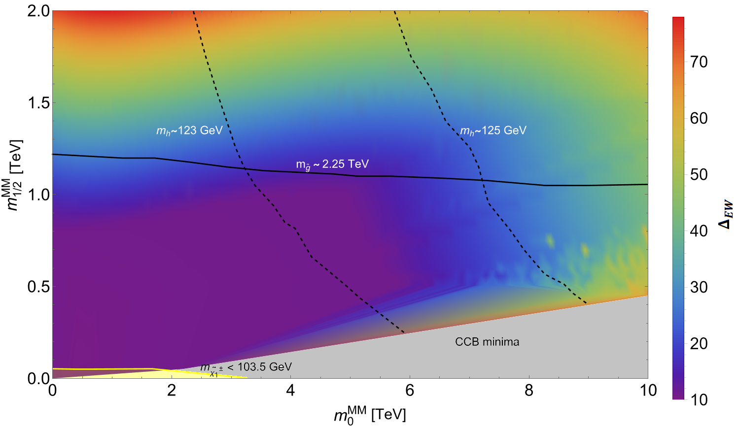
Figure 18: Plot of naturalness measure $\Delta_{\rm EW}$ in the $m_{0}^{MM}$ vs. $m_{/2}^{MM}$ plane of the generalized mirage-mediation model for $\tan\beta=10$ with $c_{m}=c_{m3}$ and $a_{3}=1.6\sqrt{c_{m}}$. For GMM^′, we also require $\mu=200$ GeV and $m_{A}=2$ TeV. The spectrum is calculated using Isasugra.

9 Conclusions

In this paper, we have re-examined three finetuning measures which are widely used in the literature: $\Delta_{\rm BG}$, $\Delta_{\rm HS}$ and $\Delta_{\rm EW}$. A fourth, stringy naturalness, does not yet admit a quantitative measure although it may be possible in future work. These measures have been quoted vaguely to bolster opinions on future HE facilities and to set policy for future experiments. Given the situation, a critical evaluation seems necessary. While naturalness definitions such as ’t Hooft naturalness certainly apply to supersymmetry and the big hierarchy problem, in that a low scale of SUSY breaking is technically natural in that the model becomes more (super)symmetric as the SUSY breaking order parameter $\rightarrow 0$, this doesn’t apply to the Little Hierarchy which is instead concerned with the increasing mass gap between the measured value of the weak scale and the scale of soft SUSY breaking terms (which determine $m_{weak}$ via Eq. 3). For the LHP, we invoke instead the notion of practical naturalness, where all independent contributions to any observable should be comparable to or less than the measured value of the observable.

The three naturalness measures are all attempts to measure practical naturalness. The $\Delta_{\rm EW}$ measure is most conservative and unavoidable. It is model independent within a fixed matter content (such as the MSSM). It is also unambiguous. Its lessons can be immediately extracted from Eq. 3: the only superparticles required at the weak scale are the various higgsinos whose mass derives from the SUSY conserving $\mu$ parameter. While the value of $\mu$ is frequently tuned in Eq. 3 such as to give the measured value of $m_{Z}$, its physics origin is rather obscure and may or may not be directly related to SUSY breaking. Of the remaining superparticle contributions to the weak scale, all are suppressed by loop factors times mass-squared factors in Eq. 3 so that the sparticles can lie in the TeV-to-multiTeV range at little cost to naturalness. In the string landscape picture, in fact, there is a statistical draw to large soft terms so long as their contributions to the weak scale are not too large: this then predicts $m_{h}\sim 125$ GeV with sparticles typically beyond present reach of LHC[103, 126].

The traditional $\Delta_{\rm BG}$ measure which instead famously placed upper bounds on all sparticles of just a few hundred GeV suffers from the ambiguity of what to take as free parameters in the log-derivative measure. While the commonly used SUSY EFTs adopt a variety of “parameters of ignorance”, it is noted that in more specific models the soft terms are all correlated (in our universe). Taking multiple soft parameters as the $p_{i}$ in $\Delta_{\rm BG}$ leads to overestimates of finetuning by factors of up to 500-1000 as compared to $\Delta_{\rm EW}$. Also, the measure $\Delta_{\rm BG}$ is rather complicated to compute, so we have embedded its numerical evaluation into the publicly available code DEW4SLHA which computes all three finetuning measures given an input SUSY Les Houches Accord file. By combining dependent soft terms, then $\Delta_{\rm BG}$ reduces to the tree level value of $\Delta_{\rm EW}$.

The measure $\Delta_{HS}$ which computes $\sim\delta m_{H_{u}}^{2}/m_{weak}^{2}$ is found to overestimate finetuning by artificially splitting $m_{H_{u}}^{2}(weak)$ into $m_{H_{u}}^{2}(\Lambda)+\delta m_{H_{u}}^{2}$ which actually are not independent contributions to $m_{h}^{2}$. In fact, selection of appropriately broken EW symmetry requires $\delta m_{H_{u}}^{2}$ to be large or else EW symmetry is not broken. This measure, which famously predicts three third generation squarks below 500 GeV, also overestimates finetuning by up to three orders of magnitude. By combining the dependent terms $m_{H_{u}}^{2}(\Lambda)$ with $\delta m_{H_{u}}^{2}$, then $\Delta_{\rm HS}$ reduces to $\Delta_{\rm EW}$ according to Eq. 20.

Our ultimate conclusion is that the so-called naturalness crisis[127, 128] which arose from non-observation of SUSY particles at LHC is not a crisis at all, but is based on faulty estimates of finetuning by the $\Delta_{\rm BG}$ and $\Delta_{\rm HS}$ measures (which are actually inconsistent with each other). The more conservative measure $\Delta_{\rm EW}$ rules out old favorites such as the CMSSM/mSUGRA model based on naturalness, but allows for plenty of natural parameter space in models like NUHMi, nAMSB and nGMM (and of course less theoretically constrained exploratory constructs like pMSSM). In fact, the naturalness-allowed and LHC-allowed parameter space regions are precisely those which seem most prevalent from rather general considerations of the string landscape. In this light, the above natural SUSY models maintain a high degree of motivation, and are perhaps even more highly motivated than pre-LHC times due to the emergence of the string landscape. Thus, policy decisions for future HEP facilities, especially future accelerators, should bear this resolution in mind in that it may be that we just need a much more energetic collider for the discovery of superpartners.

References

- [1] E. Witten, Dynamical Breaking of Supersymmetry, Nucl. Phys. B 188 (1981) 513. doi:10.1016/0550-3213(81)90006-7.
- [2] R. K. Kaul, Gauge Hierarchy in a Supersymmetric Model, Phys. Lett. B 109 (1982) 19–24. doi:10.1016/0370-2693(82)90453-1.
- [3] S. Dimopoulos, S. Raby, F. Wilczek, Supersymmetry and the Scale of Unification, Phys. Rev. D 24 (1981) 1681–1683. doi:10.1103/PhysRevD.24.1681.
- [4] U. Amaldi, W. de Boer, H. Furstenau, Comparison of grand unified theories with electroweak and strong coupling constants measured at LEP, Phys. Lett. B 260 (1991) 447–455. doi:10.1016/0370-2693(91)91641-8.
- [5] J. R. Ellis, S. Kelley, D. V. Nanopoulos, Probing the desert using gauge coupling unification, Phys. Lett. B 260 (1991) 131–137. doi:10.1016/0370-2693(91)90980-5.
- [6] P. Langacker, M.-x. Luo, Implications of precision electroweak experiments for , , and grand unification, Phys. Rev. D 44 (1991) 817–822. doi:10.1103/PhysRevD.44.817.
- [7] L. E. Ibanez, G. G. Ross, SU(2)-L x U(1) Symmetry Breaking as a Radiative Effect of Supersymmetry Breaking in Guts, Phys. Lett. B 110 (1982) 215–220. doi:10.1016/0370-2693(82)91239-4.
- [8] L. E. Ibanez, C. Lopez, N=1 Supergravity, the Breaking of SU(2) x U(1) and the Top Quark Mass, Phys. Lett. B 126 (1983) 54–58. doi:10.1016/0370-2693(83)90015-1.
- [9] L. Alvarez-Gaume, J. Polchinski, M. B. Wise, Minimal Low-Energy Supergravity, Nucl. Phys. B 221 (1983) 495. doi:10.1016/0550-3213(83)90591-6.
- [10] P. Slavich, et al., Higgs-mass predictions in the MSSM and beyond, Eur. Phys. J. C 81 (5) (2021) 450. arXiv:2012.15629, doi:10.1140/epjc/s10052-021-09198-2.
- [11] S. Heinemeyer, W. Hollik, G. Weiglein, L. Zeune, Implications of LHC search results on the W boson mass prediction in the MSSM, JHEP 12 (2013) 084. arXiv:1311.1663, doi:10.1007/JHEP12(2013)084.
- [12] P. Candelas, G. T. Horowitz, A. Strominger, E. Witten, Vacuum configurations for superstrings, Nucl. Phys. B 258 (1985) 46–74. doi:10.1016/0550-3213(85)90602-9.
- [13] B. S. Acharya, Supersymmetry, Ricci Flat Manifolds and the String Landscape, JHEP 08 (2020) 128. arXiv:1906.06886, doi:10.1007/JHEP08(2020)128.
- [14] J. R. Ellis, D. Ross, A Light Higgs boson would invite supersymmetry, Phys. Lett. B 506 (2001) 331–336. arXiv:hep-ph/0012067, doi:10.1016/S0370-2693(01)00156-3.
- [15] F. Vissani, Do experiments suggest a hierarchy problem?, Phys. Rev. D 57 (1998) 7027–7030. arXiv:hep-ph/9709409, doi:10.1103/PhysRevD.57.7027.
- [16] M. Farina, D. Pappadopulo, A. Strumia, A modified naturalness principle and its experimental tests, JHEP 08 (2013) 022. arXiv:1303.7244, doi:10.1007/JHEP08(2013)022.
- [17] C. K. M. Klein, Minimal radiative neutrino mass -A systematic study-, Master’s thesis, Heidelberg, Max Planck Inst. (2019).
- [18] H. M. Lee, S. Raby, M. Ratz, G. G. Ross, R. Schieren, K. Schmidt-Hoberg, P. K. S. Vaudrevange, Discrete R symmetries for the MSSM and its singlet extensions, Nucl. Phys. B 850 (2011) 1–30. arXiv:1102.3595, doi:10.1016/j.nuclphysb.2011.04.009.
- [19] H. P. Nilles, Stringy Origin of Discrete R-symmetries, PoS CORFU2016 (2017) 017. arXiv:1705.01798, doi:10.22323/1.292.0017.
- [20] H. Baer, V. Barger, D. Sengupta, Gravity safe, electroweak natural axionic solution to strong and SUSY problems, Phys. Lett. B 790 (2019) 58–63. arXiv:1810.03713, doi:10.1016/j.physletb.2019.01.007.
- [21] P. N. Bhattiprolu, S. P. Martin, High-quality axions in solutions to the problem, Phys. Rev. D 104 (5) (2021) 055014. arXiv:2106.14964, doi:10.1103/PhysRevD.104.055014.
- [22] M. Demirtas, N. Gendler, C. Long, L. McAllister, J. Moritz, PQ AxiversearXiv:2112.04503.
- [23] M. Dine, A. Kusenko, The Origin of the matter - antimatter asymmetry, Rev. Mod. Phys. 76 (2003) 1. arXiv:hep-ph/0303065, doi:10.1103/RevModPhys.76.1.
- [24] K. J. Bae, H. Baer, H. Serce, Y.-F. Zhang, Leptogenesis scenarios for natural SUSY with mixed axion-higgsino dark matter, JCAP 01 (2016) 012. arXiv:1510.00724, doi:10.1088/1475-7516/2016/01/012.
- [25] H. Baer, X. Tata, Weak scale supersymmetry: From superfields to scattering events, Cambridge University Press, 2006.
- [26] N. Craig, et al., Snowmass Theory Frontier ReportarXiv:2211.05772.
- [27] M. Narain, et al., The Future of US Particle Physics - The Snowmass 2021 Energy Frontier ReportarXiv:2211.11084.
- [28] J. R. Ellis, K. Enqvist, D. V. Nanopoulos, F. Zwirner, Observables in Low-Energy Superstring Models, Mod. Phys. Lett. A 1 (1986) 57. doi:10.1142/S0217732386000105.
- [29] R. Barbieri, G. F. Giudice, Upper Bounds on Supersymmetric Particle Masses, Nucl. Phys. B 306 (1988) 63–76. doi:10.1016/0550-3213(88)90171-X.
- [30] B. de Carlos, J. A. Casas, One loop analysis of the electroweak breaking in supersymmetric models and the fine tuning problem, Phys. Lett. B 309 (1993) 320–328. arXiv:hep-ph/9303291, doi:10.1016/0370-2693(93)90940-J.
- [31] G. W. Anderson, D. J. Castano, Naturalness and superpartner masses or when to give up on weak scale supersymmetry, Phys. Rev. D 52 (1995) 1693–1700. arXiv:hep-ph/9412322, doi:10.1103/PhysRevD.52.1693.
- [32] S. Dimopoulos, G. F. Giudice, Naturalness constraints in supersymmetric theories with nonuniversal soft terms, Phys. Lett. B 357 (1995) 573–578. arXiv:hep-ph/9507282, doi:10.1016/0370-2693(95)00961-J.
- [33] P. H. Chankowski, J. R. Ellis, S. Pokorski, The Fine tuning price of LEP, Phys. Lett. B 423 (1998) 327–336. arXiv:hep-ph/9712234, doi:10.1016/S0370-2693(98)00060-4.
- [34] P. H. Chankowski, J. R. Ellis, M. Olechowski, S. Pokorski, Haggling over the fine tuning price of LEP, Nucl. Phys. B 544 (1999) 39–63. arXiv:hep-ph/9808275, doi:10.1016/S0550-3213(99)00025-5.
- [35] M. Bastero-Gil, G. L. Kane, S. F. King, Fine tuning constraints on supergravity models, Phys. Lett. B 474 (2000) 103–112. arXiv:hep-ph/9910506, doi:10.1016/S0370-2693(00)00002-2.
- [36] H. Abe, T. Kobayashi, Y. Omura, Relaxed fine-tuning in models with non-universal gaugino masses, Phys. Rev. D 76 (2007) 015002. arXiv:hep-ph/0703044, doi:10.1103/PhysRevD.76.015002.
- [37] R. K. Ellis, et al., Physics Briefing Book: Input for the European Strategy for Particle Physics Update 2020arXiv:1910.11775.
- [38] J. N. Butler, et al., Report of the 2021 U.S. Community Study on the Future of Particle Physics (Snowmass 2021)doi:10.2172/1922503.
- [39] J. L. Feng, K. T. Matchev, T. Moroi, Multi - TeV scalars are natural in minimal supergravity, Phys. Rev. Lett. 84 (2000) 2322–2325. arXiv:hep-ph/9908309, doi:10.1103/PhysRevLett.84.2322.
- [40] J. L. Feng, K. T. Matchev, T. Moroi, Focus points and naturalness in supersymmetry, Phys. Rev. D 61 (2000) 075005. arXiv:hep-ph/9909334, doi:10.1103/PhysRevD.61.075005.
- [41] R. L. Arnowitt, P. Nath, Supersymmetry and Supergravity: Phenomenology and Grand Unification, in: 6th Summer School Jorge Andre Swieca on Nuclear Physics, 1993. arXiv:hep-ph/9309277.
- [42] G. L. Kane, C. F. Kolda, L. Roszkowski, J. D. Wells, Study of constrained minimal supersymmetry, Phys. Rev. D 49 (1994) 6173–6210. arXiv:hep-ph/9312272, doi:10.1103/PhysRevD.49.6173.
- [43] H. Baer, V. Barger, D. Mickelson, How conventional measures overestimate electroweak fine-tuning in supersymmetric theory, Phys. Rev. D 88 (9) (2013) 095013. arXiv:1309.2984, doi:10.1103/PhysRevD.88.095013.
- [44] H. Baer, V. Barger, D. Mickelson, M. Padeffke-Kirkland, SUSY models under siege: LHC constraints and electroweak fine-tuning, Phys. Rev. D 89 (11) (2014) 115019. arXiv:1404.2277, doi:10.1103/PhysRevD.89.115019.
- [45] H. Murayama, Supersymmetry phenomenology, in: ICTP Summer School in Particle Physics, 2000, pp. 296–335. arXiv:hep-ph/0002232.
- [46] R. Harnik, G. D. Kribs, D. T. Larson, H. Murayama, The Minimal supersymmetric fat Higgs model, Phys. Rev. D 70 (2004) 015002. arXiv:hep-ph/0311349, doi:10.1103/PhysRevD.70.015002.
- [47] Z. Chacko, Y. Nomura, D. Tucker-Smith, A Minimally fine-tuned supersymmetric standard model, Nucl. Phys. B 725 (2005) 207–250. arXiv:hep-ph/0504095, doi:10.1016/j.nuclphysb.2005.07.019.
- [48] R. Kitano, Y. Nomura, A Solution to the supersymmetric fine-tuning problem within the MSSM, Phys. Lett. B 631 (2005) 58–67. arXiv:hep-ph/0509039, doi:10.1016/j.physletb.2005.10.003.
- [49] R. Kitano, Y. Nomura, Supersymmetry, naturalness, and signatures at the LHC, Phys. Rev. D 73 (2006) 095004. arXiv:hep-ph/0602096, doi:10.1103/PhysRevD.73.095004.
- [50] M. Papucci, J. T. Ruderman, A. Weiler, Natural SUSY Endures, JHEP 09 (2012) 035. arXiv:1110.6926, doi:10.1007/JHEP09(2012)035.
- [51] C. Brust, A. Katz, S. Lawrence, R. Sundrum, SUSY, the Third Generation and the LHC, JHEP 03 (2012) 103. arXiv:1110.6670, doi:10.1007/JHEP03(2012)103.
- [52] H. Baer, V. Barger, P. Huang, A. Mustafayev, X. Tata, Radiative natural SUSY with a 125 GeV Higgs boson, Phys. Rev. Lett. 109 (2012) 161802. arXiv:1207.3343, doi:10.1103/PhysRevLett.109.161802.
- [53] H. Baer, V. Barger, D. Martinez, Comparison of SUSY spectra generators for natural SUSY and string landscape predictions, Eur. Phys. J. C 82 (2) (2022) 172. arXiv:2111.03096, doi:10.1140/epjc/s10052-022-10141-2.
- [54] K. L. Chan, U. Chattopadhyay, P. Nath, Naturalness, weak scale supersymmetry and the prospect for the observation of supersymmetry at the Tevatron and at the CERN LHC, Phys. Rev. D 58 (1998) 096004. arXiv:hep-ph/9710473, doi:10.1103/PhysRevD.58.096004.
- [55] M. R. Douglas, Basic results in vacuum statistics, Comptes Rendus Physique 5 (2004) 965–977. arXiv:hep-th/0409207, doi:10.1016/j.crhy.2004.09.008.
- [56] V. Agrawal, S. M. Barr, J. F. Donoghue, D. Seckel, Viable range of the mass scale of the standard model, Phys. Rev. D 57 (1998) 5480–5492. arXiv:hep-ph/9707380, doi:10.1103/PhysRevD.57.5480.
- [57] H. Baer, V. Barger, S. Salam, Naturalness versus stringy naturalness (with implications for collider and dark matter searches), Phys. Rev. Research. 1 (2019) 023001. arXiv:1906.07741, doi:10.1103/PhysRevResearch.1.023001.
- [58] P. Z. Skands, et al., SUSY Les Houches accord: Interfacing SUSY spectrum calculators, decay packages, and event generators, JHEP 07 (2004) 036. arXiv:hep-ph/0311123, doi:10.1088/1126-6708/2004/07/036.
- [59] R. L. Workman, et al., Review of Particle Physics, PTEP 2022 (2022) 083C01. doi:10.1093/ptep/ptac097.
- [60] S. K. Soni, H. A. Weldon, Analysis of the Supersymmetry Breaking Induced by N=1 Supergravity Theories, Phys. Lett. B 126 (1983) 215–219. doi:10.1016/0370-2693(83)90593-2.
- [61] V. S. Kaplunovsky, J. Louis, Model independent analysis of soft terms in effective supergravity and in string theory, Phys. Lett. B 306 (1993) 269–275. arXiv:hep-th/9303040, doi:10.1016/0370-2693(93)90078-V.
- [62] A. Brignole, L. E. Ibanez, C. Munoz, Towards a theory of soft terms for the supersymmetric Standard Model, Nucl. Phys. B 422 (1994) 125–171, [Erratum: Nucl.Phys.B 436, 747–748 (1995)]. arXiv:hep-ph/9308271, doi:10.1016/0550-3213(94)00068-9.
- [63] F. Gabbiani, E. Gabrielli, A. Masiero, L. Silvestrini, A Complete analysis of FCNC and CP constraints in general SUSY extensions of the standard model, Nucl. Phys. B 477 (1996) 321–352. arXiv:hep-ph/9604387, doi:10.1016/0550-3213(96)00390-2.
- [64] H. Baer, A. Mustafayev, S. Profumo, A. Belyaev, X. Tata, Neutralino cold dark matter in a one parameter extension of the minimal supergravity model, Phys. Rev. D 71 (2005) 095008. arXiv:hep-ph/0412059, doi:10.1103/PhysRevD.71.095008.
- [65] J. R. Ellis, K. A. Olive, Y. Santoso, The MSSM parameter space with nonuniversal Higgs masses, Phys. Lett. B 539 (2002) 107–118. arXiv:hep-ph/0204192, doi:10.1016/S0370-2693(02)02071-3.
- [66] J. R. Ellis, T. Falk, K. A. Olive, Y. Santoso, Exploration of the MSSM with nonuniversal Higgs masses, Nucl. Phys. B 652 (2003) 259–347. arXiv:hep-ph/0210205, doi:10.1016/S0550-3213(02)01144-6.
- [67] H. Baer, A. Mustafayev, S. Profumo, A. Belyaev, X. Tata, Direct, indirect and collider detection of neutralino dark matter in SUSY models with non-universal Higgs masses, JHEP 07 (2005) 065. arXiv:hep-ph/0504001, doi:10.1088/1126-6708/2005/07/065.
- [68] W. Buchmuller, K. Hamaguchi, O. Lebedev, M. Ratz, Local grand unification, in: GUSTAVOFEST: Symposium in Honor of Gustavo C. Branco: CP Violation and the Flavor Puzzle, 2005, pp. 143–156. arXiv:hep-ph/0512326.
- [69] H. P. Nilles, S. Ramos-Sanchez, P. K. S. Vaudrevange, Local Grand Unification and String Theory, AIP Conf. Proc. 1200 (1) (2010) 226–234. arXiv:0909.3948, doi:10.1063/1.3327561.
- [70] H. P. Nilles, P. K. S. Vaudrevange, Geography of Fields in Extra Dimensions: String Theory Lessons for Particle Physics, Mod. Phys. Lett. A 30 (10) (2015) 1530008. arXiv:1403.1597, doi:10.1142/S0217732315300086.
- [71] A. Pomarol, D. Tommasini, Horizontal symmetries for the supersymmetric flavor problem, Nucl. Phys. B 466 (1996) 3–24. arXiv:hep-ph/9507462, doi:10.1016/0550-3213(96)00074-0.
- [72] H. Baer, V. Barger, D. Sengupta, Landscape solution to the SUSY flavor and CP problems, Phys. Rev. Res. 1 (3) (2019) 033179. arXiv:1910.00090, doi:10.1103/PhysRevResearch.1.033179.
- [73] L. Randall, R. Sundrum, Out of this world supersymmetry breaking, Nucl. Phys. B 557 (1999) 79–118. arXiv:hep-th/9810155, doi:10.1016/S0550-3213(99)00359-4.
- [74] G. F. Giudice, M. A. Luty, H. Murayama, R. Rattazzi, Gaugino mass without singlets, JHEP 12 (1998) 027. arXiv:hep-ph/9810442, doi:10.1088/1126-6708/1998/12/027.
- [75] H. Baer, V. Barger, D. Sengupta, Anomaly mediated SUSY breaking model retrofitted for naturalness, Phys. Rev. D 98 (1) (2018) 015039. arXiv:1801.09730, doi:10.1103/PhysRevD.98.015039.
- [76] K. Choi, A. Falkowski, H. P. Nilles, M. Olechowski, Soft supersymmetry breaking in KKLT flux compactification, Nucl. Phys. B 718 (2005) 113–133. arXiv:hep-th/0503216, doi:10.1016/j.nuclphysb.2005.04.032.
- [77] H. Baer, V. Barger, H. Serce, X. Tata, Natural generalized mirage mediation, Phys. Rev. D 94 (11) (2016) 115017. arXiv:1610.06205, doi:10.1103/PhysRevD.94.115017.
- [78] G. ’t Hooft, Naturalness, chiral symmetry, and spontaneous chiral symmetry breaking, NATO Sci. Ser. B 59 (1980) 135–157. doi:10.1007/978-1-4684-7571-5_9.
- [79] R. Barbieri, A. Strumia, The ’LEP paradox’, in: 4th Rencontres du Vietnam: Physics at Extreme Energies (Particle Physics and Astrophysics), 2000. arXiv:hep-ph/0007265.
- [80] A. Birkedal, Z. Chacko, M. K. Gaillard, Little supersymmetry and the supersymmetric little hierarchy problem, JHEP 10 (2004) 036. arXiv:hep-ph/0404197, doi:10.1088/1126-6708/2004/10/036.
- [81] A. Canepa, Searches for Supersymmetry at the Large Hadron Collider, Rev. Phys. 4 (2019) 100033. doi:10.1016/j.revip.2019.100033.
- [82] H. Baer, V. Barger, M. Savoy, Upper bounds on sparticle masses from naturalness or how to disprove weak scale supersymmetry, Phys. Rev. D 93 (3) (2016) 035016. arXiv:1509.02929, doi:10.1103/PhysRevD.93.035016.
- [83] M. J. G. Veltman, The Infrared - Ultraviolet Connection, Acta Phys. Polon. B 12 (1981) 437.
- [84] L. Susskind, Dynamics of Spontaneous Symmetry Breaking in the Weinberg-Salam Theory, Phys. Rev. D 20 (1979) 2619–2625. doi:10.1103/PhysRevD.20.2619.
- [85] M. K. Gaillard, B. W. Lee, Rare Decay Modes of the K-Mesons in Gauge Theories, Phys. Rev. D 10 (1974) 897. doi:10.1103/PhysRevD.10.897.
- [86] J. L. Feng, Naturalness and the Status of Supersymmetry, Ann. Rev. Nucl. Part. Sci. 63 (2013) 351–382. arXiv:1302.6587, doi:10.1146/annurev-nucl-102010-130447.
- [87] G. F. Giudice, Naturally Speaking: The Naturalness Criterion and Physics at the LHC (2008) 155–178arXiv:0801.2562, doi:10.1142/9789812779762_0010.
- [88] L. E. Ibanez, C. Lopez, C. Munoz, The Low-Energy Supersymmetric Spectrum According to N=1 Supergravity Guts, Nucl. Phys. B 256 (1985) 218–252. doi:10.1016/0550-3213(85)90393-1.
- [89] A. Lleyda, C. Munoz, Nonuniversal soft scalar masses in supersymmetric theories, Phys. Lett. B 317 (1993) 82–91. arXiv:hep-ph/9308208, doi:10.1016/0370-2693(93)91574-7.
- [90] S. P. Martin, Compressed supersymmetry and natural neutralino dark matter from top squark-mediated annihilation to top quarks, Phys. Rev. D 75 (2007) 115005. arXiv:hep-ph/0703097, doi:10.1103/PhysRevD.75.115005.
- [91] S. P. Martin, M. T. Vaughn, Two loop renormalization group equations for soft supersymmetry breaking couplings, Phys. Rev. D 50 (1994) 2282, [Erratum: Phys.Rev.D 78, 039903 (2008)]. arXiv:hep-ph/9311340, doi:10.1103/PhysRevD.50.2282.
- [92] B. C. Allanach, J. P. J. Hetherington, M. A. Parker, B. R. Webber, Naturalness reach of the large hadron collider in minimal supergravity, JHEP 08 (2000) 017. arXiv:hep-ph/0005186, doi:10.1088/1126-6708/2000/08/017.
- [93] M. T. Grisaru, W. Siegel, M. Roček, Improved methods for supergraphs, Nucl. Phys. B 159 (1979) 429–450. doi:10.1016/0550-3213(79)90344-4.
- [94] K. J. Bae, H. Baer, N. Nagata, H. Serce, Prospects for Higgs coupling measurements in SUSY with radiatively-driven naturalness, Phys. Rev. D 92 (3) (2015) 035006. arXiv:1505.03541, doi:10.1103/PhysRevD.92.035006.
- [95] H. Baer, V. Barger, P. Huang, D. Mickelson, A. Mustafayev, X. Tata, Post-LHC7 fine-tuning in the minimal supergravity/CMSSM model with a 125 GeV Higgs boson, Phys. Rev. D 87 (3) (2013) 035017. arXiv:1210.3019, doi:10.1103/PhysRevD.87.035017.
- [96] H. Baer, V. Barger, M. Savoy, Supergravity gauge theories strike back: There is no crisis for SUSY but a new collider may be required for discovery, Phys. Scripta 90 (2015) 068003. arXiv:1502.04127, doi:10.1088/0031-8949/90/6/068003.
- [97] H. Baer, V. Barger, M. Savoy, H. Serce, The Higgs mass and natural supersymmetric spectrum from the landscape, Phys. Lett. B 758 (2016) 113–117. arXiv:1602.07697, doi:10.1016/j.physletb.2016.05.010.
- [98] H. Baer, V. Barger, P. Huang, D. Mickelson, A. Mustafayev, X. Tata, Radiative natural supersymmetry: Reconciling electroweak fine-tuning and the Higgs boson mass, Phys. Rev. D 87 (11) (2013) 115028. arXiv:1212.2655, doi:10.1103/PhysRevD.87.115028.
- [99] A. Dedes, P. Slavich, Two loop corrections to radiative electroweak symmetry breaking in the MSSM, Nucl. Phys. B 657 (2003) 333–354. arXiv:hep-ph/0212132, doi:10.1016/S0550-3213(03)00173-1.
- [100] H. Baer, V. Barger, J. S. Gainer, H. Serce, X. Tata, Reach of the high-energy LHC for gluinos and top squarks in SUSY models with light Higgsinos, Phys. Rev. D 96 (11) (2017) 115008. arXiv:1708.09054, doi:10.1103/PhysRevD.96.115008.
- [101] H. Baer, V. Barger, S. Salam, H. Serce, Supersymmetric particle and Higgs boson masses from the landscape: Dynamical versus spontaneous supersymmetry breaking, Phys. Rev. D 104 (11) (2021) 115025. arXiv:2103.12123, doi:10.1103/PhysRevD.104.115025.
- [102] M. R. Douglas, Statistical analysis of the supersymmetry breaking scalearXiv:hep-th/0405279.
- [103] H. Baer, V. Barger, H. Serce, K. Sinha, Higgs and superparticle mass predictions from the landscape, JHEP 03 (2018) 002. arXiv:1712.01399, doi:10.1007/JHEP03(2018)002.
- [104] G. F. Giudice, R. Rattazzi, Living Dangerously with Low-Energy Supersymmetry, Nucl. Phys. B 757 (2006) 19–46. arXiv:hep-ph/0606105, doi:10.1016/j.nuclphysb.2006.07.031.
- [105] N. Arkani-Hamed, S. Dimopoulos, S. Kachru, Predictive landscapes and new physics at a TeVarXiv:hep-th/0501082.
- [106] B. C. Allanach, SOFTSUSY: a program for calculating supersymmetric spectra, Comput. Phys. Commun. 143 (2002) 305–331. arXiv:hep-ph/0104145, doi:10.1016/S0010-4655(01)00460-X.
- [107] N. Arkani-Hamed, A. Delgado, G. F. Giudice, The Well-tempered neutralino, Nucl. Phys. B 741 (2006) 108–130. arXiv:hep-ph/0601041, doi:10.1016/j.nuclphysb.2006.02.010.
- [108] H. Baer, A. Mustafayev, E.-K. Park, X. Tata, Target dark matter detection rates in models with a well-tempered neutralino, JCAP 01 (2007) 017. arXiv:hep-ph/0611387, doi:10.1088/1475-7516/2007/01/017.
- [109] H. Baer, V. Barger, H. Serce, SUSY under siege from direct and indirect WIMP detection experiments, Phys. Rev. D 94 (11) (2016) 115019. arXiv:1609.06735, doi:10.1103/PhysRevD.94.115019.
- [110] M. Badziak, M. Olechowski, P. Szczerbiak, Is well-tempered neutralino in MSSM still alive after 2016 LUX results?, Phys. Lett. B 770 (2017) 226–235. arXiv:1701.05869, doi:10.1016/j.physletb.2017.04.059.
- [111] S. Profumo, T. Stefaniak, L. Stephenson Haskins, The Not-So-Well Tempered Neutralino, Phys. Rev. D 96 (5) (2017) 055018. arXiv:1706.08537, doi:10.1103/PhysRevD.96.055018.
- [112] E. Aprile, et al., Dark Matter Search Results from a One Ton-Year Exposure of XENON1T, Phys. Rev. Lett. 121 (11) (2018) 111302. arXiv:1805.12562, doi:10.1103/PhysRevLett.121.111302.
- [113] J. Aalbers, et al., First Dark Matter Search Results from the LUX-ZEPLIN (LZ) ExperimentarXiv:2207.03764.
- [114] H. Bahl, T. Hahn, S. Heinemeyer, W. Hollik, S. Paßehr, H. Rzehak, G. Weiglein, Precision calculations in the MSSM Higgs-boson sector with FeynHiggs 2.14, Comput. Phys. Commun. 249 (2020) 107099. arXiv:1811.09073, doi:10.1016/j.cpc.2019.107099.
- [115] F. E. Paige, S. D. Protopopescu, H. Baer, X. Tata, ISAJET 7.69: A Monte Carlo event generator for pp, anti-p p, and e+e- reactionsarXiv:hep-ph/0312045.
- [116] T. Cohen, M. Lisanti, A. Pierce, T. R. Slatyer, Wino Dark Matter Under Siege, JCAP 10 (2013) 061. arXiv:1307.4082, doi:10.1088/1475-7516/2013/10/061.
- [117] J. Fan, M. Reece, In Wino Veritas? Indirect Searches Shed Light on Neutralino Dark Matter, JHEP 10 (2013) 124. arXiv:1307.4400, doi:10.1007/JHEP10(2013)124.
- [118] A. Arbey, M. Battaglia, A. Djouadi, F. Mahmoudi, J. Quevillon, Implications of a 125 GeV Higgs for supersymmetric models, Phys. Lett. B 708 (2012) 162–169. arXiv:1112.3028, doi:10.1016/j.physletb.2012.01.053.
- [119] H. Baer, V. Barger, A. Mustafayev, Neutralino dark matter in mSUGRA/CMSSM with a 125 GeV light Higgs scalar, JHEP 05 (2012) 091. arXiv:1202.4038, doi:10.1007/JHEP05(2012)091.
- [120] J. D. Wells, PeV-scale supersymmetry, Phys. Rev. D 71 (2005) 015013. arXiv:hep-ph/0411041, doi:10.1103/PhysRevD.71.015013.
- [121] S. Kachru, R. Kallosh, A. D. Linde, S. P. Trivedi, De Sitter vacua in string theory, Phys. Rev. D 68 (2003) 046005. arXiv:hep-th/0301240, doi:10.1103/PhysRevD.68.046005.
- [122] A. Falkowski, O. Lebedev, Y. Mambrini, SUSY phenomenology of KKLT flux compactifications, JHEP 11 (2005) 034. arXiv:hep-ph/0507110, doi:10.1088/1126-6708/2005/11/034.
- [123] K. Choi, K. S. Jeong, T. Kobayashi, K.-i. Okumura, TeV Scale Mirage Mediation and Natural Little SUSY Hierarchy, Phys. Rev. D 75 (2007) 095012. arXiv:hep-ph/0612258, doi:10.1103/PhysRevD.75.095012.
- [124] H. Baer, V. Barger, D. Sengupta, Mirage mediation from the landscape, Phys. Rev. Res. 2 (1) (2020) 013346. arXiv:1912.01672, doi:10.1103/PhysRevResearch.2.013346.
- [125] K. J. Bae, H. Baer, V. Barger, D. Sengupta, Revisiting the SUSY problem and its solutions in the LHC era, Phys. Rev. D 99 (11) (2019) 115027. arXiv:1902.10748, doi:10.1103/PhysRevD.99.115027.
- [126] H. Baer, V. Barger, S. Salam, D. Sengupta, K. Sinha, Status of weak scale supersymmetry after LHC Run 2 and ton-scale noble liquid WIMP searches, Eur. Phys. J. ST 229 (21) (2020) 3085–3141. arXiv:2002.03013, doi:10.1140/epjst/e2020-000020-x.
- [127] J. Lykken, M. Spiropulu, Supersymmetry and the Crisis in Physics, Sci. Am. 310N5 (2014) 36–39.
- [128] M. Dine, Naturalness Under Stress, Ann. Rev. Nucl. Part. Sci. 65 (2015) 43–62. arXiv:1501.01035, doi:10.1146/annurev-nucl-102014-022053.