Quantum Random Number Generator Based on LED

Abstract

Quantum Random Number Generators (QRNGs) produce random numbers based on the intrinsic probability nature of quantum mechanics, making them True Random Number Generators (TRNGs). In this paper, we design and fabricate an embedded QRNG that produces random numbers based on fluctuations of spontaneous emission in a Light-Emitting Diode (LED). Additionally, a new perspective on the randomness of the recombination process in a LED is introduced that is consistent with experimental results. To achieve a robust and reliable QRNG, we compare some usual post-processing methods and select the best one for a real-time device. This device could pass NIST tests, the output speed is 1 Mbit/s and the randomness of the output data is invariant in time.

Keywords: Real-Time Quantum Random Number Generator, Spontaneous Emission, Beer-Lambert Law

I Introduction

This century can be considered the beginning of the rapid development and dissemination of quantum information technology in almost all scientific and utility fields. Meanwhile, random numbers play an important role in many aspects of information technology  Meteopolis ; Bennett_Brassard ; Schneier . Applications of random numbers include symmetric key cryptography Metropolis_2 , Monte Carlo simulation Dynes , transaction protection Bustard , and key distribution systems Symul , will be more important in the era of quantum technology.

Traditionally, pseudo-random number generators (pseudo-RNGs) were based on deterministic algorithms but could not generate truly random numbers with information-theoretically provable randomness. On the other hand, quantum random number generators (QRNGs) can generate truly random numbers from the essentially probabilistic nature of quantum processes and can also provide higher bit rates instead of physical random number generators Schmidt .

To date, various practical protocols for QRNGs have been proposed, such as QRNG-based photon counting Nie ; Jennewein ; Dynes , Raman scattering Bustard_Raman , vacuum fluctuations Shen ; Gabriel , amplified spontaneous emission Li , radioactive decay Alkassar , and laser phase noise Nie ; Qi . References Mannalath ; Ma ; Jacak are available to the reader for further information.

In this work, we experimentally demonstrate a simple, inexpensive, and real-time QRNG based on the spontaneous emission of an LED and easily accessible at high speed.

In the following, we will discuss the theoretical background of our QRNG device in section II. Then, we will demonstrate the physical setup and introduce our post-processing procedures in section III. Finally, we will present and discuss the experiment outcomes in the section  IV.

II Theory

II.1 Theoretical Background

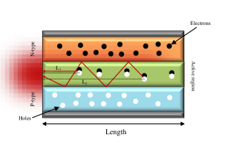
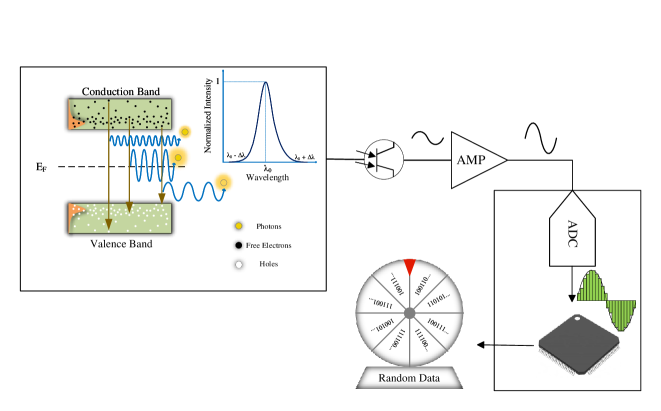
Figure 1: (a) The process of light emission from an LED involves the application of a suitable voltage, which causes electrons and holes to recombine randomly in the active region. It is worth noting that the length of output for each photon is different. (b) Schematic of the built QRNG. The enclosure size is 16 × 12 × 6 $\operatorname{cm}^{3}$. (c) Diagram of QRNG. The LED’s energy diagram illustrates the density of state for electrons and holes, with a varying absorption coefficient for each photon due to different frequencies. After emission, the photon is absorbed by the photodiode, and the output electrical signal is amplified, then digitized by an ADC and processed through a microprocessor.

Our study aims to amplify the random fluctuations in LED light output for use in a QRNG. Before exploring the experimental setup, we show that the light intensity variations in an LED are intrinsically random and probabilistic by analyzing the light-emitting mechanism in an LED in 2 steps. In the first step, we illustrate the broadening wavelength in LED using Fermi’s golden rule, then justify the temporal light intensity variation using the Beer-Lambert law.

In the case of an LED, we can apply Fermi’s golden rule to derive the transition probability between the conduction and valence bands, as expressed Nasser :

$$w_{\operatorname{cv}}=\Big{\lvert}\frac{1}{i\hbar}\int_{0}^{t}\langle\psi_{v}|H_{\operatorname{int}}|\psi_{c}\rangle e^{i\omega_{\operatorname{cv}}t^{\prime}}dt^{\prime}\Big{\rvert}^{2}$$ (1)

Here, $\psi_{c}$ and $\psi_{v}$ represent arbitrary states in the conduction and valence bands respectively, and $\hbar\omega_{\operatorname{cv}}$ is their energy difference. To determine the transition probability in an LED, the applied voltage on the LED, represented by $H_{\operatorname{int}}=-eE=V$, where $E$ denotes the applied electric field and $V$ is the LED voltage Chaung .

Fermi’s golden rule can explain the phenomenon of frequency broadening in an LED, but it may not be able to describe the changes in intensity over time. To bridge this gap, we rely on the Beer-Lambert law, which connects Fermi’s golden rule to temporal intensity fluctuations. According to the Beer-Lambert law expressed in Eq. (2), the intensity of light $I_{0}$ passing through an object decreases exponentially with the passed distance

$$I=I_{0}e^{-\alpha L}$$ (2)

where $\alpha$ represents the absorption coefficient of the object and $L$ denotes the distance traveled by the light. As shown in Fig. 1, for each photon generated by an LED, the distance traveled may vary. Thus, Eq. (2) shows that there would be fluctuations in light intensity if there is a variation in $\alpha$ or $L$. To describe the light intensity fluctuations, we analyzed $\alpha$ and $L$ parameters. To derive the $\alpha$ in an LED, we focus on the photon generation in the active region. The interaction Hamiltonian for a generated photon into the active region is Nasser :

$$H_{\operatorname{int}}^{\operatorname{photon}}=-E_{0}{\operatorname{cos}}({\bf q}{\bf{r}}-\omega t){\bf{e}}_{q}{\bf{d}}$$ (3)

where $E_{0}$, $\bf q$, $\omega$, and ${\bf{e}}_{q}$ are the electric field amplitude, wavenumber, angular frequency, and polarization unit vector of the generated photon, respectively, and $\bf{d}=-\operatorname{e}\bf{r}$ denotes the light-induced electric field dipole moment. Restricting the treatment to the dipole approximation, we obtain:

$$\langle\psi_{c}|H_{\operatorname{int}}|\psi_{v}\rangle=-\frac{E_{0}}{2}(e^{-i\omega t}+e^{i\omega t}){\bf{d}}_{\operatorname{cv}}$$ (4)

which ${\bf{d}}_{\operatorname{cv}}=\langle\psi_{c}|{\bf{e}}_{q}{\bf{d}}|\psi_{v}\rangle$ is the dipole element for transition between state $\psi_{c}$ and $\psi_{v}$. On the other hand, the absorption coefficient can be defined as Chaung :

$$\alpha=\frac{w_{\operatorname{cv}}\hbar\omega}{tS}$$ (5)

where $S$ represents the Poynting vector, and $w_{\operatorname{cv}}/t$ is the transition probability per unit of time or the transition rate probability. Regarding Eqs. (1), (3)-(5), one can derive $\alpha$ as Nasser :

$$\alpha=\frac{\omega}{\pi n_{b}c}|{\bf{d}}_{\operatorname{cv}}|^{2}\int_{0}^{\infty}4\pi k^{2}\delta(\hbar\omega_{\operatorname{cv}}-\hbar\omega)~{}dk$$ (6)

Eq. (6) gives the absorption coefficient in terms of the density of states and the dipole element where $n_{b}$ and c, are the background refractive index and the speed of light, respectively.

In the next step, to investigate the effect of $\alpha$ on the light intensity, we assume $L$ is constant. This assumption is valid since some generated photons are closer to the LED aperture, and some are farther. In this manner, we define an effective optical length $L_{\operatorname{eff}}$ for the photons, and regarding Eq. (2) we achieve:

$$I=I_{0}e^{-\alpha L_{\operatorname{eff}}}$$ (7)

This suggests that light intensity fluctuations may arise from $\alpha$ variations, and if $\alpha$ has a normal distribution, $I$ should have a log-normal distribution. On the other hand, the relation between $\alpha$ and wavelength $\lambda$ for different materials is Chaung :

$$\alpha=\frac{4\pi\kappa}{\lambda}$$ (8)

where $\kappa$ is the extinction coefficient. For any LED which $\alpha L_{\operatorname{eff}}<<1$, we can approximate Chaung :

$$I\approx I_{0}(1-\alpha L_{\operatorname{eff}})$$ (9)

This indicates that the light intensity follows the distribution of the absorption coefficient. Considering Eqs. (5)-(6), the $\alpha$ depends on the transition rate probability and the energy of the generated photons. Both of these terms are random and make fluctuations in the light intensity. For example, wavelength broadening has been shown in Fig. 1, which can directly cause a variation in the light intensity. Thus the intensity fluctuations in an LED are inherently probable and cannot be predicted, making it a reliable source in QRNG.

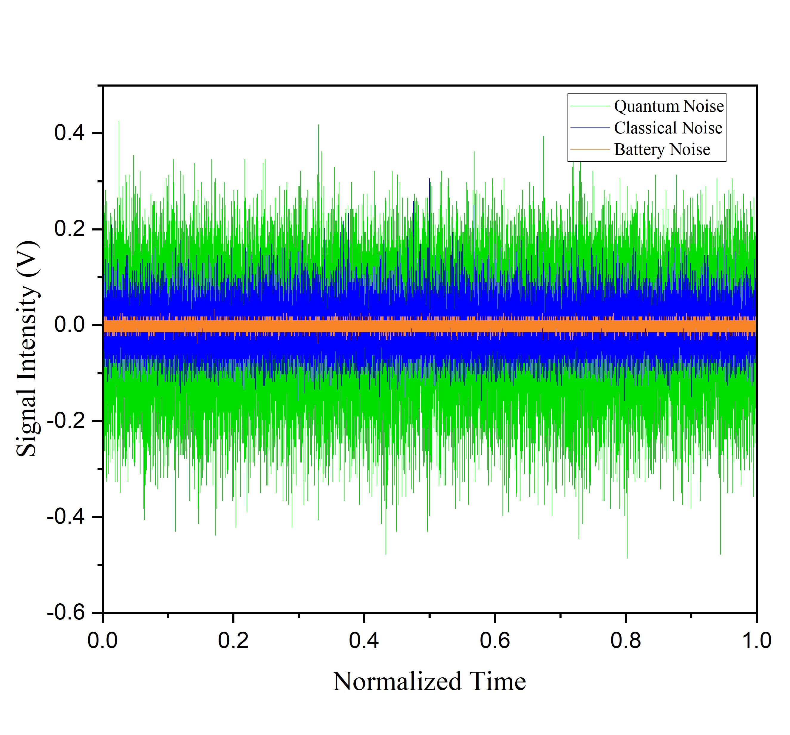
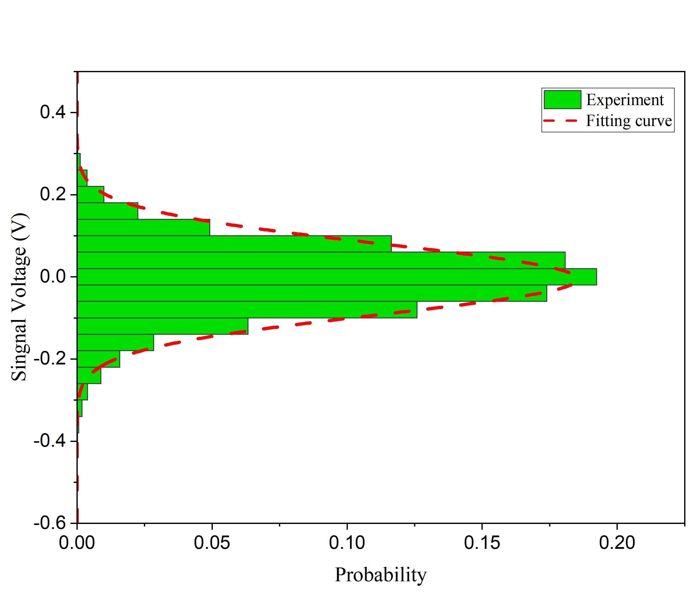
Figure 2: (a) Temporal waveforms of the LED and amplifier circuit’s quantum signal and classic noise, where quantum noise is the prevailing factor. The green curve indicates the quantum signal, while the blue curve represents the amplified classical noise (shot noise and environmental noise), and the orange curve illustrates the amplified battery noise. (b) The histogram distribution of the signal voltage is represented by the green bars, with the dashed lines indicating a well-fitted Gaussian distribution.

II.2 Spontaneous Emission

This section discusses cases where LED noise is more dominant than other noises. We aim to obtain the conditions in which the Signal to Noise Ratio (SNR) and min-entropy of the QRNG device are at their highest values. To determine the SNR for LED noise, we use the following formula:

$$SNR=\frac{A_{\operatorname{PD}}}{A_{\operatorname{CS}}}$$ (10)

$A_{\operatorname{PD}}$ is the amplitude of the signal received from LED through the photodetector (PD) and illustrates the quantum signal, and $A_{\operatorname{CS}}$ is the amplitude of overall classical noise, assuming shot noise is the primary noise source. It should be mentioned that classical noise is measured when the LED is not operating. $A_{\operatorname{PD}}$ is directly related to the light intensity that reaches the PD:

$$A_{\operatorname{PD}}\approx I_{0}\alpha L_{\operatorname{eff}}$$ (11)

By substituting Eq. (11) into Eq (10), we get:

$$SNR=C_{0}\frac{I_{0}\alpha L_{\operatorname{eff}}}{A_{\operatorname{CS}}}$$ (12)

which $C_{0}$ is a constant. The numerator of Eq. (12) is affected only by $\alpha$ since other parameters are constant. Eq. (1) shows that $\alpha$ is determined only by voltage, and since the LED voltage is constant, the numerator does not change across different currents. However, $A_{\operatorname{CS}}$ increases as the current increases Chaung . Thus, increasing the current leads to a decrease in both the SNR and the min-entropy in the LED-based QRNG , and decreasing the current should increase the SNR and min-entropy.

Our experimental results, which will be described in section IV , are in agreement with the above theoretical framework.

III Experimental Methods

III.1 Physical Setup

The integrated optical and electronic components into an enclosure and the conceptual design are shown in Fig. 1 and  1, respectively. The detailed design block diagram of the QRNG module comprises three main parts. First, the quantum entropy source (LED). Second, the amplification of the signal received from LED by an amplifier (AMP). Finally, digitizing the amplified signal by an Analog-to-Digital Converter (ADC) with 12-bit resolution and 4 MSa/s sample rate and applying a post-processing procedure using a microprocessor. As demonstrated in Fig. 2, the temporal waveforms of signal and noise are measured, indicating that the quantum signal is dominant. The output signal oscillates irregularly, and shows good randomness of intensity fluctuation. The signal distribution is given by the green histogram in Fig. 2, and the Poisson distribution and symmetry are demonstrated by comparing them with the red fitting curve Sanguinetti .

III.2 Post-Processing Procedures

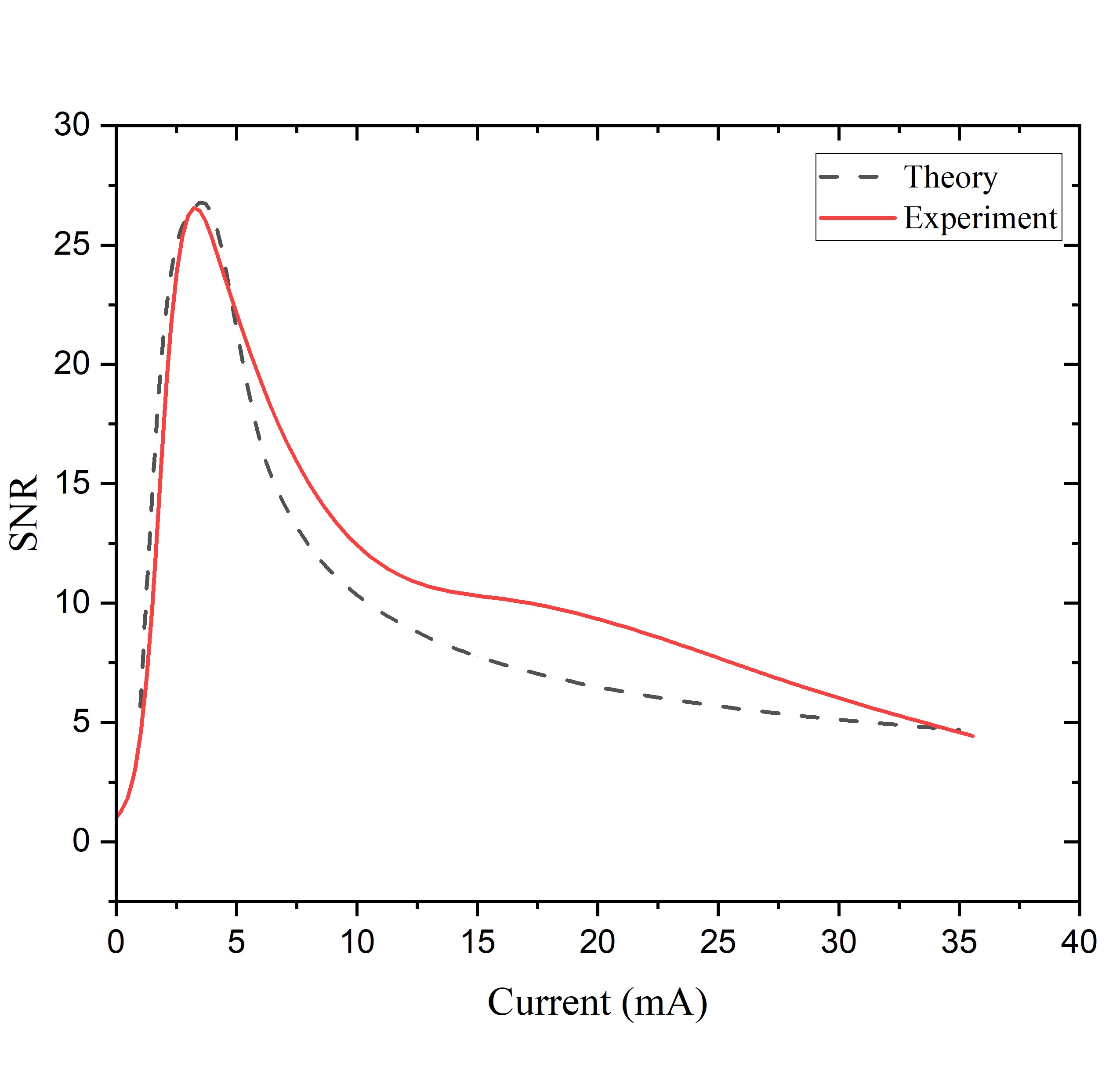
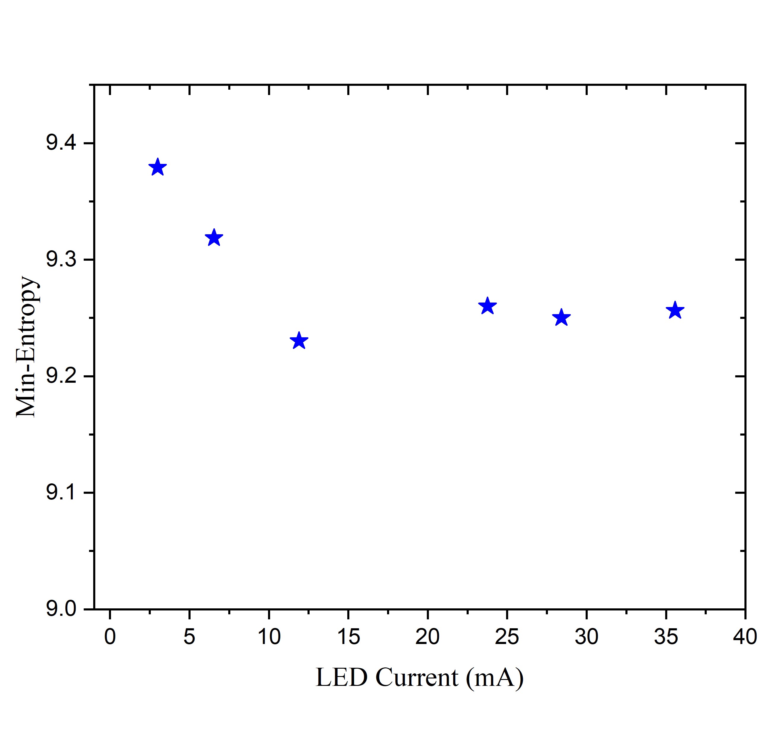
Figure 3: (a) The figure presents the ratio of quantum signal to classical noise, revealing that as the current decreases, the SNR increases as per theoretical predictions. (b) Min-entropy after FIR operation versus LED current bias. It shows the highest min-entropy occurs when the spontaneous emission is dominant.

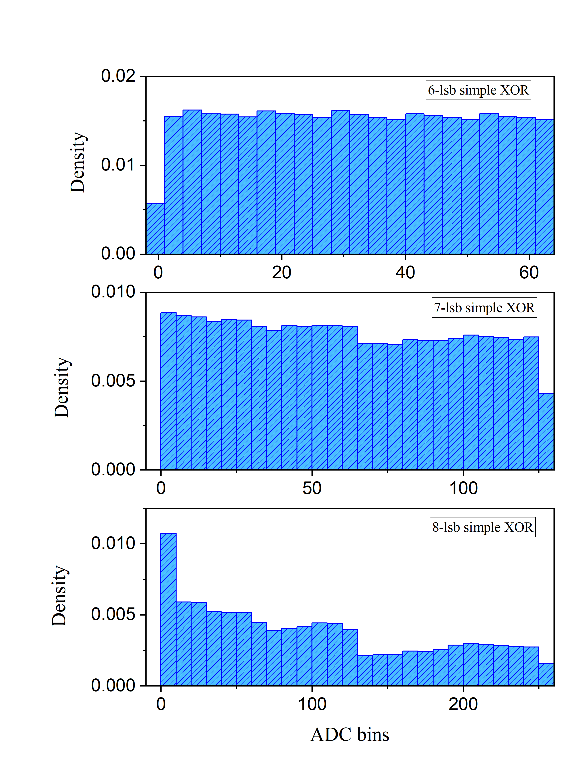
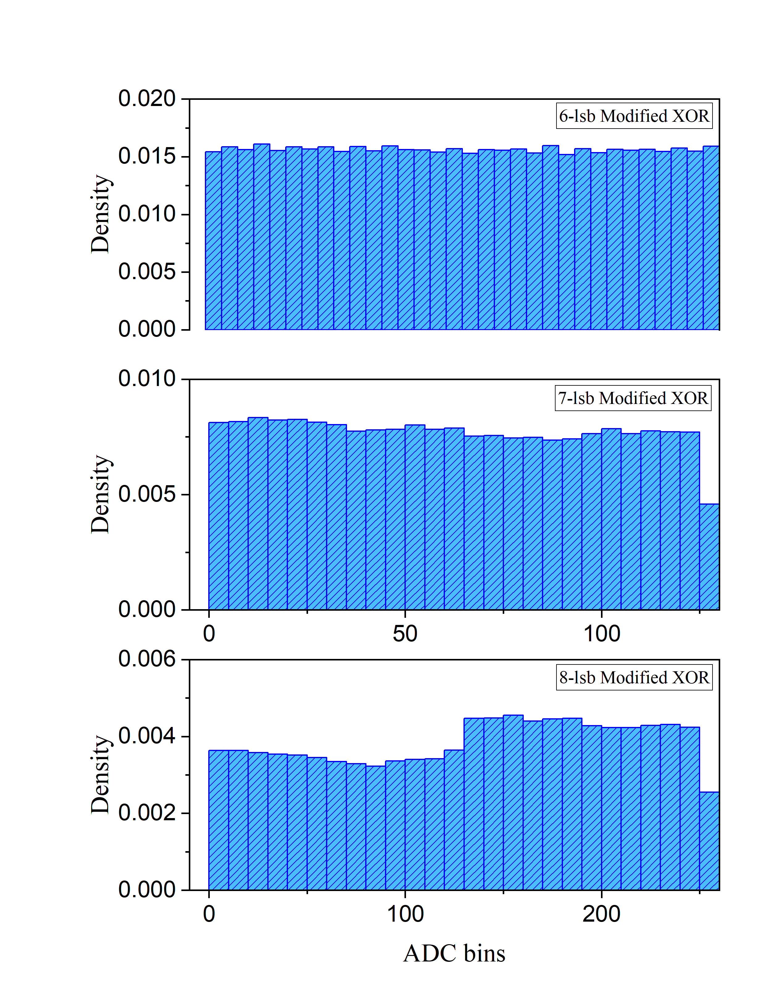
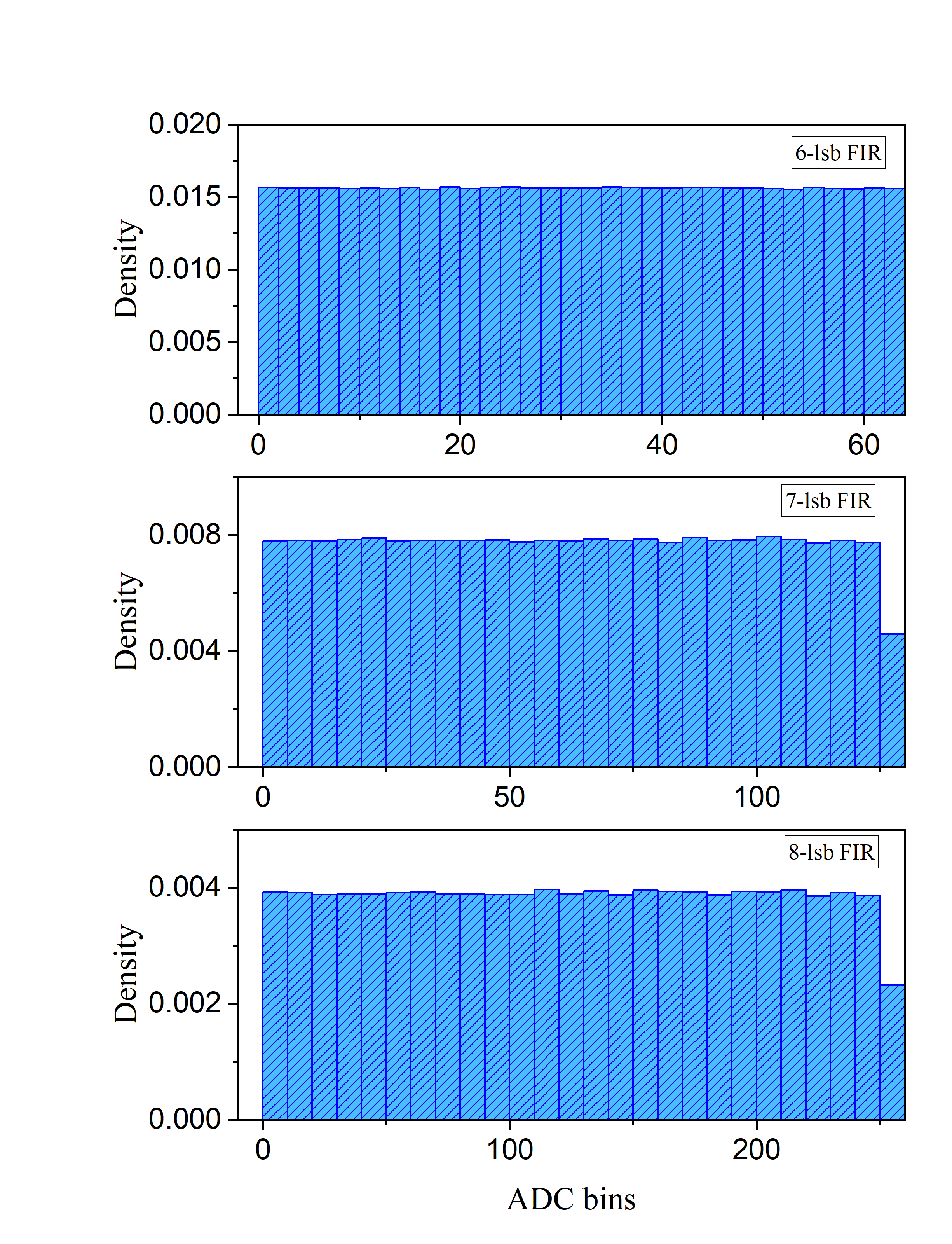
Figure 4: The probability distribution of three post-processing approaches with different m-lsb values (m=6, m=7, m=8): (a) Simple XOR, (b) Modified XOR, and (c) FIR. The FIR method produces a perfectly uniform distribution, while the other two approaches exhibit some non-uniformity.

The purpose of standard RNGs is to generate a random uniform string, in which the raw numbers are processed to obtain a good-quality output with a uniform distribution. Thus, we aimed to convert the Poisson distribution of the random number generator to a uniform distribution using post-processing, and we explored three different methods to achieve this. The first approach involved a simple XOR (S-XOR) processing technique, where a single number from the ADC was XORed with the $k_{\operatorname{th}}$ number following it. The second approach was the modified XOR (M-XOR) method, where the output of the ADC was XORed with a shift-rotated version of itself and then XORed with the $k_{\operatorname{th}}$ number following it. The last approach that is effective in increasing the entropy of random numbers is the finite impulse response (FIR) method Ifeachor . The FIR method involves taking a weighted sum of past input samples, as described by Eq. (13), to analyze the input signal. This can help to reduce any unwanted noise or interference in the signal, leading to a higher-quality output. Studies have shown that using the FIR method can also increase the min-entropy, or the lowest possible entropy, of the generated random numbers. This is because the method effectively extracts randomness from the raw input data, producing a more unpredictable output Marangon . This technique consists in transforming a raw integer sample $x(n)$ into an unbiased one $y(n)$, by means of the relation:

$$y(n)=\sum_{i=0}^{M}b_{i}x(n-i)$$ (13)

where $b_{i}=\frac{M!}{i!(M-i)!}$ and M is the number of raw samples. After every technique, we have taken m-Least Significant Bit (m-LSB).

In the next section, we report the results of SNR at different currents and demonstrated the obtained results for different post-processing techniques.

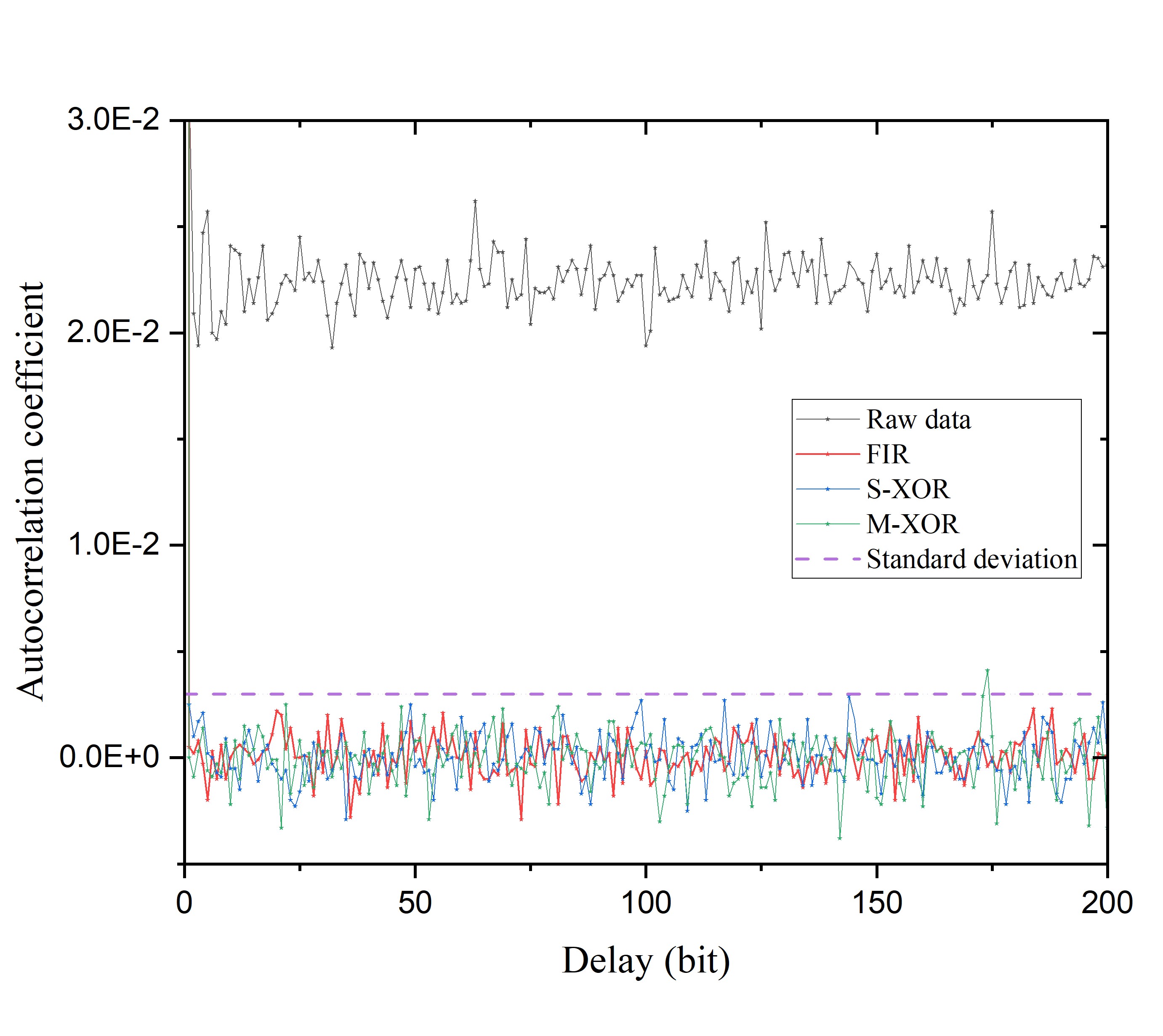
Figure 5: The autocorrelation coefficient for four different datasets: raw data, S-XOR, M-XOR, and FIR. The standard deviation is denoted by the dashed line.

IV Results and Discussion

One of the objectives of this experiment was to optimize the min-entropy of a QRNG setup. The min-entropy is a measure of the randomness of a sequence of numbers, and to obtain high-quality random numbers, we should maximize the min-entropy Metropolis_2 ; Dynes . To achieve this, we varied the current supplied to the LED and measured the SNR of the quantum and classical signals. Our findings demonstrated that at low currents, the quantum signal dominates, while at higher currents, the classical noise dominates, as shown in Fig. 3 and predicted by Eq. (12). Therefore, we determined the optimal current range where the quantum signal is the strongest and the classical noise is minimal. By maximizing the SNR in this range, we were able to achieve the highest min-entropy in our setup. The min-entropy versus LED current has been shown in Fig. 3 which indicates that for lower currents, the SNR and min-entropy are at the highest values.

To establish a robust and reliable device we compare and evaluate three different post-processing procedures for real-time embedded systems that were introduced in the previous section. The suitability of these methods was assessed based on their processing time and ability to produce uniformly distributed random numbers that pass the National Institute of Standards and Technology (NIST) randomness test NIST1 ; NIST . The findings of this study are presented in Figs. 4 and 5, which illustrate the m-lsb values obtained through the application of three distinct post-processing methods, as well as the autocorrelation between the resultant data. As it has been shown in Fig. 5, the autocorrelation of post-processed data is below the standard deviation means the random data are not correlated Xu . The FIR method produced a uniform probability distribution at 10-lsb and passed the NIST randomness test, while the S-XOR and M-XOR methods produced uniformity at 5-lsb and 6-lsb, respectively. Table 1 presents the results of the NIST randomness test for each approach. Our findings indicate that the S-XOR approach did not pass some of the NIST tests, as presented in Table 1. Therefore, caution is necessary when relying solely on the uniform distribution achieved by the S-XOR approach.

Table 1: Performance comparison of NIST results for S-XOR, M-XOR, and FIR methods.

Statistical Tests	FIR	M-XOR	S-XOR
Frequency	Success	Success	Failed
Block Frequency	Success	Success	Failed
Runs	Success	Success	Failed
Longest Run	Success	Success	Failed
Rank	Success	Success	Success
FFT	Success	Success	Success
Non-Overlapping Template	Success	Success	Success
Overlapping Template	Success	Success	Success
Universal	Success	Success	Success
Linear Complexity	Success	Success	Success
Serial	Success	Success	Success
Approximate Entropy	Success	Success	Success
Cumulative Sums	Success	Success	Failed
Random Excursions	Success	Success	Failed
Random Excursions Variant	Success	Success	Failed

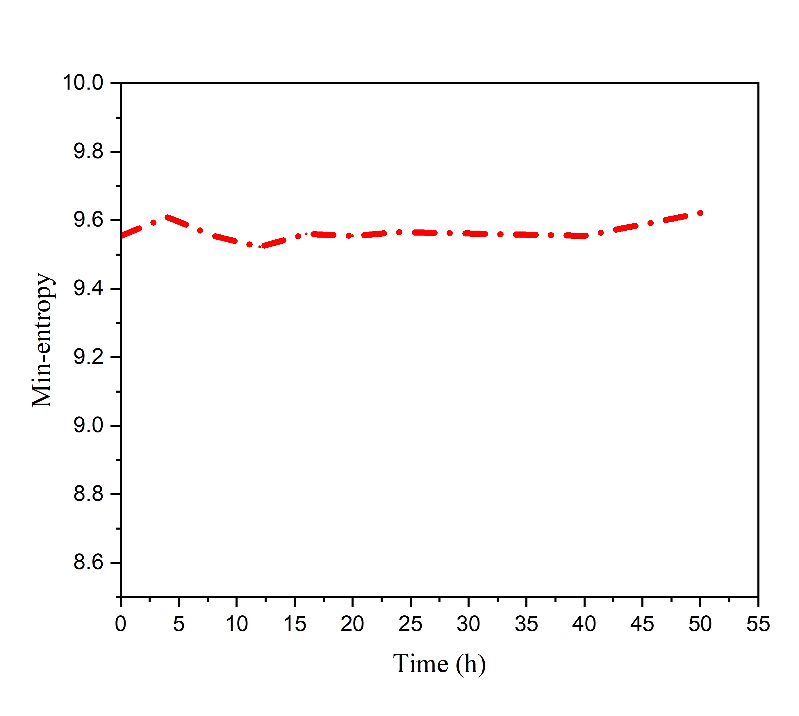
Figure 6: The figure illustrates the relationship between min-entropy and time, indicating the device’s dependable and consistent production of randomness over time.

The results assert that the FIR method is the most suitable approach for post-processing in real-time embedded systems. This method has been found to increase the min-entropy of the random data, thereby improving the reliability and robustness of the device. Following a comparative analysis of three alternative methods, we have selected the FIR method for use in our device. To further evaluate the performance of our device, we conducted a series of tests, including temperature tests to assess the impact of temperature on device performance, bias current tests to evaluate the effect of varying bias currents on device performance, and time duration tests to determine the stability of device performance over time. These tests have provided valuable insights into the effectiveness and reliability of the FIR method for post-processing in real-time embedded systems. The findings presented in Fig. 6 demonstrate the variation of the min-entropy of random data over time. The results show that the min-entropy remains almost constant, indicating that the fabricated device is robust and reliable over time. Additionally, a temperature test was performed to assess the device’s reliability and robustness against varying temperatures which displays that the device performs well and maintains its reliability and robustness even under temperature fluctuations.

Finally, our QRNG device now reaches a data bit rate of 1 Mb/s and has the potential to attain higher rates by integrating additional LEDs in a parallel configuration.

V Conclusion

We have fabricated a durable, low-power, cost-effective QRNG uses LED spontaneous emission. Our findings demonstrate that, at lower currents, the quantum noise dominates and increases the SNR and min-entropy. To the best of our knowledge, our work establishes the connection between Fermi’s golden rule and the temporal fluctuations of light intensity of an LED for the first time. Moreover, we evaluated various post-processing methods and discovered that the FIR approach is the most reliable and yields the highest min-entropy outcomes. Our device maintains a stable min-entropy over time and under variable temperatures, operates at a real-time rate of 1 Mb/s, and has passed all the NIST tests. These results provide a promising route for building efficient and practical QRNGs with potentially high bit rates.

References

- (1) N. Meteopolis and S. Ulam, The monte carlo method, J. Am. Stat. Assoc., 44, (1949)
- (2) C. H. Bennett and G. Brassard, Quantum cryptography: Public key distribution and coin tossing, Proc. Int. Conf., (1984)
- (3) B. Schneier, Applied Cryptography: Protocols, Algorithms, and Source Code in C, John Wiley and Sons, (1995)
- (4) N. Metropolis, et al., E. Equation of state calculations by fast computing machines, J. Chem. Phys., 21, (1953)
- (5) J. F. Dynes, et al., A high speed, post-processing free, quantum random number generator, Appl. Phys. Lett., 93, (2008)
- (6) P. J. Bustard, et al., Quantum random number generator based on twin beams, Opt. Express, 21, (2013)
- (7) T. Symul, et al., Real time demonstration of high bitrate quantum random number generation with coherent laser light, Appl. Phys. Lett., 98, (2011)
- (8) H. Schmidt, Quantum mechanical random-number generator, J. Appl. Phys., 41, (1970)
- (9) T. Jennewein, et al., A fast and compact quantum random number generator, Rev. Sci. Instrum., 71, (2000)
- (10) Y. Q. Nie, et al., 68 Gbps quantum random number generation by measuring laser phase fluctuations, Rev. Sci. Instrum., 86, (2015)
- (11) P. J. Bustard, et al., Quantum random bit generation using energy fluctuations in stimulated Raman scattering, Opt. Express, 21, (2011)
- (12) Y. Shen, et al., Practical quantum random number generator based on measuring the shot noise of vacuum states, Phys. Rev. A, 81, (2010)
- (13) C. Gabriel, et al., A generator for unique quantum random numbers based on vacuum states, Nat. Photon., 4, (2010)
- (14) X. Li, et al., Scalable parallel physical random number generator based on a superluminescent LED, Opt. Lett., 36, (2011)
- (15) A. Alkassar, et al., Obtaining true-random binary numbers from a weak radioactive source, Computational Science and Its Applications, (2005)
- (16) B. Qi, et al., High-speed quantum random number generation by measuring phase noise of a single-mode laser, Opt. Lett., 35, (2010)
- (17) V. Mannalath, et al., A comprehensive review of quantum random number generators: Concepts, classification and the origin of randomness, arXiv:2203.00261, (2022)
- (18) X. Ma, et al., Quantum random number generation, Npj Quantum Inf., 2, (2016)
- (19) M. Jacak, et al., Quantum generators of random numbers, Sci. Rep., 11, (2021)
- (20) N. Peyghambarian, Introduction to Semiconductor Optics, Pearson College Div, (1993)
- (21) S. L. Chaung, Physics of Photonic Devices, Wiley, (2009)
- (22) B. Sanguinetti, et al., Quantum random number generation on a mobile phone, Phys. Rev. X, 4, (2014)
- (23) S. C. Ifeachor and B. W. Jervis, Digital Signal Processing: A Practical Approach, Pearson Education, (2002)
- (24) D. G. Marangon, et al., Long term test of a fast and compact quantum random number generator, Optica, 36, (2018)
- (25) National Institute of Standards and Technology, Security Requirements for Cryptographic Modules. CSRC — NIST, (2002)
-
(26)
NIST: Random Number Generation and Testing: https://nvlpubs.nist.gov/nistpubs/legacy/sp/
nistspecialpublication800-22r1a.pdf - (27) F. Xu, et al., Ultrafast quantum random number generation based on quantum phase fluctuations, Opt. Express, 20, (2012)