The GNAR-edge model: A network autoregressive model for networks with time-varying edge weights

Abstract

In economic and financial applications, there is often the need for analysing multivariate time series, comprising of time series for a range of quantities. In some applications such complex systems can be associated with some underlying network describing pairwise relationships among the quantities. Accounting for the underlying network structure for the analysis of this type of multivariate time series is required for assessing estimation error and can be particularly informative for forecasting. Our work is motivated by a dataset consisting of time series of industry-to-industry transactions. In this example, pairwise relationships between Standard Industrial Classification (SIC) codes can be represented using a network, with SIC codes as nodes and pairwise transactions between SIC codes as edges, while the observed time series of the amounts of the transactions for each pair of SIC codes can be regarded as time-varying weights on the edges. Inspired by Knight et al., (2020), we introduce the GNAR-edge model which allows modelling of multiple time series utilising the network structure, assuming that each edge weight depends not only on its past values, but also on past values of its neighbouring edges, for a range of neighbourhood stages. The method is validated through simulations. Results from the implementation of the GNAR-edge model on the real industry-to-industry data show good fitting and predictive performance of the model. The predictive performance is improved when sparsifying the network using a lead-lag analysis and thresholding edges according to a lead-lag score.

Keywords: networks, autoregressive model, multiple time series, network time series, lead-lag relationships

Disclaimer

The views expressed are those of the authors and may not reflect the views of the Office for National Statistics or the wider UK Government.

1 Introduction

Multivariate correlated time series commonly arise in many contexts, such as in economics and finance. In some applications, such correlated time series can be represented by an underlying network with multivariate time series on the edges describing pairwise relationships among the quantities. This paper illustrates that network representations of this type can be informative for explaining the data through parameter estimation, as well as for forecasting.

There are two common approaches for modelling multivariate time series systems. The first, simple and fast approach is to model each time series individually, using an autoregressive model Box et al., (2015). This approach lacks in leveraging information from the whole time series system jointly. The second approach is to jointly model a Vector Autoregressive (VAR) model (Lütkepohl,, 2005; Tsay,, 2013). This approach uses information from the entire time series system; a key limitation is the complexity of the model with respect to the parameters under estimation, which increases quadratically with increasing number of time series (see Section 3 for details). In light of this limitation, a range of studies have focused on imposing sparsity on the coefficients of the classic VAR model, with the goal to allow statistical inference for multivariate time series in high-dimensional settings. Among the most commonly used shrinkage approaches are Lasso-based regularization approaches, introducing a penalty in the optimisation problem for estimating the model parameters; the penalty provides control over the number of parameters that are meaningful to be incorporated in each setting. Notably, in the recent study of Nicholson et al., (2020), the authors introduce a Lasso-type approach for sparsifying the classic VAR model using a hierarchical lag group penalty function, called HLAG, that leverages the ordered structure of the lag coefficients in a VAR. Another recent study by Dallakyan et al., (2022) utilises time series graphical Lasso, extending the two-stage inference framework for sparse VAR models introduced by Davis et al., (2016). Alternative methods for dimensionality reduction for the VAR model involve the use of information criteria (Tsay,, 2013; Lütkepohl,, 2005), Bayesian methods (Koop,, 2013) and factor models (Bernanke et al.,, 2005), to name a few. A concise review of the different sparsity approaches in statistics literature is presented in Nicholson et al., (2020). With the Lasso-type approaches, the reduction in the number of parameters of the VAR model is performed in the inference step of the unrestricted VAR model. When the multivariate time series is known to have network structure, then this information can be utilised in advance in the VAR model, forming a restricted VAR model which is tailored to network time series, as we discuss next.

A commonly studied type of multivariate time series associated with a network structure, is a time series observed on the nodes of a network. Recent studies have focused on modelling such network time series, with the goal of a downstream prediction task. Zhu et al., (2017) introduces the network vector autoregressive model (NAR), which is a special version of the classical VAR model that incorporates network information explicitly. Specifically, Zhu et al., (2017) assumes that the value of a node $i$ at time $t$ depends not only on previous values of the node, but also on previous values of nodes which are neighbours of node $i$, as well as a set of node-specific covariates. In this setting, Zhu et al., (2017) considers only nodes which are followed by node $i$ via a directed edge. Knight et al., (2020) extends this idea by introducing the generalized network autoregressive (GNAR) model that also incorporates the effect of larger neighborhood sizes for each node $i$. Both studies assume a fixed network structure across time. A network autoregressive model accounting for a time-varying network structure is proposed by Kang et al., (2021), who obtain a class of restricted, concatenated VAR models, and infer a dynamic network that changes for each VAR sub-model assumed. In a similar setup, Spencer et al., (2015) introduces an autoregressive model for nodal time series, restricted to the case of Directed Acyclic Graphs (DAG), while in the study of Armillotta and Fokianos, (2021) the authors propose a Poisson network autoregressive model for modelling count time series observed on the nodes of a network. Some special cases of network autoregressive models for nodal time series which extend the aforementioned studies, are proposed by Zhu et al., (2019) who develop a network quantile autoregressive model; Zhu et al., (2020) propose a different inferential framework for modelling social networks using a multivariate spatial autoregressive model, and Chen et al., (2023) incorporate information about the community structure of the network in the autoregressive model. A slightly different approach to the aforementioned studies is that of Sioofy Khoojine et al., (2021); motivated by predicting COVID-19 infection, the authors develop a network autoregressive model for time series on nodes of star-shaped networks only.

Our work is related to the type of multivariate time series considered in the aforementioned studies, with the key difference that in our setting, the time series are observed on the edges of the network as time-varying weights, rather than the nodes. Specifically, we are motivated by a data set consisting of time series of industry-to-industry transactions, aggregated to Standard Industrial Classification (SIC) codes; SIC codes classify companies according to the nature of their business Companies House, (2018). In this data, pairwise relationships between SIC codes can be represented using a network with SIC codes as nodes, while the observed time series for each pair of SIC codes can be regarded as time-varying edge weights. Inspired by the studies of Zhu et al., (2017) and Knight et al., (2020), we introduce the GNAR-edge model that allows to capture network information by incorporating the effect of neighbouring edges in the model. Similarly to the studies of Zhu et al., (2017) and Knight et al., (2020) and motivated by the real data application, we assume that the network structure is fixed over time.

There are a few related studies which take a network-based approach. One class of class of studies which is related to our work is the analysis of dynamic networks, which focuses on modelling the evolving structure of a network. In the dynamic networks literature, various models have been developed that extend models from the static network literature, such as Exponential Random Graphs (ERGM) Krivitsky and Handcock, (2014); Hanneke et al., (2010), latent space models Durante and Dunson, (2016); Sarkar and Moore, (2005) and Stochastic Block Models (SBM) Matias and Miele, (2017); Ludkin et al., (2018); Fu et al., (2009); Jiang et al., (2020); Pensky, (2019). The study of Suveges and Olhede, (2023) uses a logistic autoregressive model utilising a community structure on the edges rather than the nodes of the graph. Two main differences of our work to the aforementioned studies are that (i) most of the studies focus on unweighted graphs, while we consider weights on the edges of the network which carry the signal, and (ii) we assume a fixed network structure with only the weights varying across time.

In the computer science literature, related work includes research on traffic congestion in transportation, through the use of systems such as Global Positioning Systems which can collect data from vehicles traversing road segments; a review can be found for example in Abdi and Amrit, (2021). In this context, networks arise as road networks with nodes representing road junctions and edges representing road segments. In Menelaou et al., (2018), the authors propose two alternative approaches for predicting the travel times of vehicles for road segments (edges), using an Exponential Moving Average and a Multiple Linear Regression predictor. The key differences of our approach to the one proposed in Menelaou et al., (2018) are that (i) we propose an autoregressive model (ii) Menelaou et al., (2018) consider only direct neighbours to a segment while we allow nodes which are more than distance 1 away; we call these higher-stage neighbours and (iii) we further propose a technique for sparsifying the underlying network using lead-lag analysis of the time series.

To model traffic flow it is natural to incorporate a spatial component in the model. Min and Wynter, (2011) use spatial correlations among locations to model traffic flow time series. Salamanis et al., (2015) extends the spatio-temporal autoregressive model by providing an alternative for the spatial correlation component, which now does not necessarily have a geographical interpretation, but rather includes information about neighbouring nodes that are detected using a Breadth First Search (BFS) algorithm. This study exhibits two main differences to our approach; (i) Salamanis et al., (2015) model nodal time series, thus, the resulting approach is more related to the approaches proposed by Zhu et al., (2017) and Knight et al., (2020); and (ii) the proposed model includes only lags up to size 2 and neighbouring nodes up to stage 10, formulated specifically for the application of interest, and thus does not provide a general framework for network time series.

Main contribution.

In this paper, we provide a general framework for time series modelling and prediction for networks with fixed structure and time-varying edge weights, fully leveraging the topology of the network through identifying and incorporating information about neighbouring linkages into the model. Our approach is flexible as it can be implemented on any type of network, with no restriction on the specification of the lags and neighbour stages. Furthermore, our approach has good statistical properties while allowing for uncertainty quantification through confidence intervals.

Paper structure.

The rest of the paper is organised as follows. In Section 2, we describe the real data set that has motivated the proposed model. In Section 3, we provide the necessary background to our approach. Section 4 introduces the problem setup and the GNAR-edge model. In Section 5, we perform a range of synthetic data experiments to validate the GNAR-edge model performance in parameter estimation and prediction, also under model misspecification, and present its efficacy against baseline models. In Section 6, we fit the GNAR-edge model on the real data, and introduce a framework for network sparsification that exploits time series information. This framework uses scores from a lead-lag analysis to threshold edges. We conclude with discussion and future work in Section 7. The Supplementary material contains additional details of the experiments and real data results.

Code and synthetic data experiments are available at

https://github.com/mantziou/GNAR-edge-model.

2 A motivating data example

This work is motivated by an anonymised and aggregated UK business payments dataset made available to the Office for National Statistics by Pay.UK and Vocalink, respectively the operator of and infrastructure provider to the UK’s retail interbank payment systems. Individual firm-to-firm transactions are aggregated to two-digit SIC codes, as per latest list updated by Companies House on 9 January 2018 Companies House, (2018), using a method developed by the Office for National Statistics. Excluding Activities of extraterritorial organisations and bodies and Dormant Company there are 90 two-digit SIC codes. The resulting dataset consists of multiple time series of monthly transactions between two-digit SIC codes for a recording period starting from January 2015 and ending in July 2022, having thus 91 time stamps.

This data can be associated with an underlying network structure, imposed by the pairs of transactions between SIC codes as nodes that comprise an edge list. The presence, although not the weight, of an edge is taken to be constant acrosss time. We record an edge between two SIC codes when there are no more than 85 zero payments observed in the time series for the recording period, thus allowing for at most 6 of the 91 months to have a no payment recorded between the two SIC codes. The resulting network has 90 nodes representing SIC codes, and 7,152 directed edges (out of 8100 possible edges) representing transactions. Transactions can occur within the same industry, hence, we observe self-loops in the network. The sizes of the transactions observed across time are represented as time-varying weights on the edges of the network. Thus there are two key assumptions under this construction: first, the network has a fixed structure, and second, the network has time-varying edge weights. On two-digit SIC aggregation level, the resulting time series comprise of mostly non-zero transactions. One could instead have constructed a different network for each month, but there would be only very few changes in the network structure with respect to edges appearing or vanishing across time, while adding considerable complexity to the model. In light of this feature of the data, the assumption of a fixed network structure is natural for our problem.

Transactions between SIC codes can reflect the economic conditions in a country Buda et al., (2022). For example, big disruptions can have an effect on the economy, and subsequently on transactions occurring between firms Carvalho et al., (2021). The ability to accurately predict future transactions could play a key role in identifying, navigating, and potentially even preventing the occurrence of such effects. In addition, accounting for the underlying network formed by the associations between economic entities may assist in capturing the propagation of shocks. For this type of data set, the research questions for the observed multivariate time series which we address in this paper are as follows.

• Can we predict the sizes of future transactions accurately and with theoretical guarantees?

• Can we leverage the information encoded by the underlying network structure to improve the forecasting task?

In Section 4, we introduce the GNAR-edge model that allows one to perform prediction under the assumption that a transaction occurring at time $t$ between two SIC codes is influenced not only by past transactions between the same two SIC codes but also by past values of neighbour transactions. First we recall the general VAR model and outline its special case introduced by Knight et al., (2020) that utilises a network structure.

3 Background

In the multiple time series setting, we observe time series of some fixed length $T$ for different variables $i=1,\ldots,K$. Let $X_{i}^{t}$ denote the value of variable $i$ at time $t=1,\ldots,T$. The VAR(L) model is an autoregressive model with maximum lag $L$, that has the following linear form,

$$X_{i}^{t}=v_{i}+\alpha_{i_{1,1}}X_{1}^{t-1}+\alpha_{i_{2,1}}X_{2}^{t-1}+\ldots+\alpha_{i_{K,1}}X_{K}^{t-1}+\ldots+\alpha_{i_{1,L}}X_{1}^{t-L}+\ldots+\alpha_{i_{K,L}}X_{K}^{t-L}+u_{i}^{t},\quad i=1,\ldots,K$$ (1)

with intercept $v_{i}$, coefficients $\alpha_{i_{j,l}},j=1,\ldots,K,l=1,\ldots,L$, and the innovations $(u_{1}^{t},\ldots,u_{K}^{t}),$ $t=1,\ldots,T$, being a $K-$dimensional white noise. Equation 1 can be written compactly in vector form as

$$\boldsymbol{X_{t}}=\boldsymbol{v}+\sum_{l=1}^{L}\boldsymbol{A_{l}}\boldsymbol{X_{t-l}}+\boldsymbol{U_{t}}$$ (2)

with $\boldsymbol{X_{t}}=(X_{1}^{t},\ldots,X_{K}^{t})$, $\boldsymbol{v}=(v_{1},\ldots,v_{K})$ denoting a $K-$dimensional vector of intercepts, $\boldsymbol{A_{l}}$ denoting a $(K\times K)$ coefficient matrix with $(i,j)$ entry $\alpha_{i_{j,l}}$ and $\boldsymbol{U_{t}}=(u_{1}^{t},\ldots,u_{K}^{t})$. Under the VAR model, for each lag $l$ we regress on all variables $i=1,\ldots,K$; with fixed maximum lag $L$ there are $LK^{2}$ coefficients $a_{i_{j,l}}$ to estimate, which explains the high complexity of the VAR model which is $\mathcal{O}(K^{2})$.

In the case where a network structure is known for the variables, to reduce the complexity of the model Knight et al., (2020) propose a restricted case of the VAR model that utilises the neighbourhood structure of the network, as follows. Let $\mathcal{G}=(V,E)$ denote a graph where $V=\{1,\ldots,n\}$ represents the set of $n$ nodes, and $E$ represents the set of edges with $E=\{(i,j)|i\rightarrow j;i,j\in V\}$ for a directed graph, or $E=\{(i,j)|i\leftrightarrow j;i,j\in V\}$ for an undirected graph. For simplicity here we restrict attention to directed graphs; the adaptation to undirected graphs is straightforward. In Knight et al., (2020), a graph describes relationships among the set of node variables for which the time series are observed, thus $X_{i}^{t}$ represents the value of node $i$ at time $t$. They assume that future values of a time series observed on node $i$ depend not only on past values of that node, but also on past values of times series observed on nodes which are neighbours of node $i$; the set of 1-stage neighbour nodes of node $i$ is defined as $\mathcal{N}^{(1)}(i)=\{j\in V/\{i\}:i\rightarrow j\}$ and for $r\geq 2$ the set of $r$-stage neighbours of $i$ is defined as

$$\mathcal{N}^{(r)}(i)=\mathcal{N}\{\mathcal{N}^{(r-1)}(i)\}/[\{\cup_{q=1}^{r-1}\mathcal{N}^{(q)}(i)\}\cup\{i\}].$$

The model allows for edge or node covariates $c\in\{1,\ldots,C\}$, for some $C\in\mathbb{N}$, which can be viewed as node or edge types. Knight et al., (2020) then introduce a generalised autoregressive model with maximum lag $L$ and maximum stage $R_{l}$ for lag $l\in\{1,\ldots,L\}$ as follows,

$$X^{t}_{i}=\sum_{l=1}^{L}\Bigg{(}\alpha_{i,l}X^{t-l}_{i}+\sum_{c=1}^{C}\sum_{r=1}^{R_{l}}\beta_{l,r,c}\sum_{q\in\mathcal{N}_{t}^{r}(i)}w_{i,q,c}X^{t-l}_{q}\Bigg{)}+u_{i}^{t},$$ (3)

with $w_{i,q,c}$ representing connection weights that depend on the size of the neighbour set and which could encode edge-weight information in the case of weighted graphs. As the authors only provide a framework for a static graph across time, despite the general form provided in (3), the $r$-stage neighbour set $\mathcal{N}^{r}(i)$ is not indexed by time.

In our work, we take a similar approach as Knight et al., (2020) but consider instead the case where time series are observed on the edges of a fixed graph, rather than on the nodes. This model requires the notion of $r$-stage neighbouring edges for an edge $\{i,j\}$, which is introduced in the next section.

4 A network autoregressive model for edge time series

4.1 Problem set-up and notation

Motivated by the real data application, our setting considers directed networks (graphs) on $n$ nodes with possible self-loops; we denote the adjacency matrix of graph $\mathcal{G}$ by $A$. We let $N=n^{2}$ denote the number of possible edges and $|E|=K$ the number of edges in the static network. Our model assumes that $\mathcal{G}$ is fixed, but that there is a time varying process on $E$ which can be viewed as a matrix-valued process $V_{t},t\geq 0$ of non-negative weights. We denote by $\boldsymbol{X^{t}}=A\odot V_{t}$ the time-varying weighted adjacency matrix of the network time series at time $t$, with $\odot$ denoting the element-wise product, or Hadamard product, between matrices $A$ and $V_{t}$. Thus, $X^{t}_{ij}$ represents the weight of edge $\{i,j\}$ at time $t$.

We define the set of 1-stage neighbouring edges for some edge $\{i,j\}$ as the set of all edges which are incident to at least one of the nodes $i,j$; formally,

$$\mathcal{N}^{1}(\{i,j\})=\{\{k,l\}\in\delta^{+}(i)\cup\delta^{-}(i)\cup\delta^{+}(j)\cup\delta^{-}(j):\{k,l\}\neq\{i,j\}\}$$

with $\delta^{+}(\cdot),\delta^{-}(\cdot)$ denoting the sets of outgoing and incoming edges of a node, respectively. For $r\geq 2$ we define the set of $r$-stage neighbouring edges of the edge $\{i,j\}$ as the set

$$\mathcal{N}^{r}(\{i,j\})=\mathcal{N}\{\mathcal{N}^{r-1}(\{i,j\})\}/[\{\cup_{q=1}^{r-1}\mathcal{N}^{q}(\{i,j\})\}\cup\{\{i,j\}\}].$$

As the network is fixed, these sets do not depend on time. Figure 1 shows an example of the 1-stage and 2-stage neighbours for the edge $1\rightarrow 2$ in a toy graph.

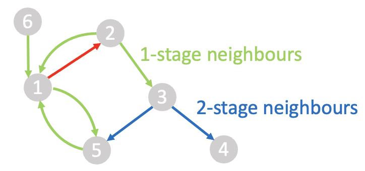
Figure 1: An example of 1-stage and 2-stage neighbours for edge $1\rightarrow 2$.

4.2 The GNAR-edge model

Inspired by Knight et al., (2020), we assume that the weight $X^{t}_{ij}$ of an edge between nodes $i,j$ at time $t$ depends not only on its past values, but also on past values of its neighbouring edges. Thus, the GNAR-edge model has the following general form for maximum lag $L$

$$X^{t}_{ij}=\sum_{l=1}^{L}\Bigg{(}\alpha_{ij,l}X^{t-l}_{ij}+\sum_{r=1}^{R_{l}}\beta_{l,r}\sum_{m,n:\{m,n\}\in\mathcal{N}^{r}(\{i,j\})}w_{ij,mn}X^{t-l}_{mn}\Bigg{)}+u_{ij}^{t},$$ (4)

with $\alpha_{ij,l}$ denoting the standard autoregressive parameters at lag $l$ for edge $\{i,j\}$, $\beta_{l,r}$ denoting the parameters for the effect of $r$-stage neighbouring edges at lag $l$, $w_{ij,mn}=|N^{r}(\{i,j\})|^{-1}$ denoting the normalising weight for $X_{mn}^{t-l}$ which equally weights all neighbouring edges of edge $\{i,j\}$ and the innovations $u_{ij}^{t}$ denoting white noise with mean 0 and variance $\sigma^{2}$. The model in equation 4 is abbreviated as GNAR-edge($L$,[$R_{1}$,…,$R_{L}$]) where the first argument $L$ denotes the maximum lag and each element of the second argument $R_{l}$ denotes the maximum stage neighbours for lag $l$.

We note that the weights $w_{ij,mn}$ do not necessarily need to reflect the size of the neighbour set but could perhaps reflect associations between edge time series measured by some correlation function, or by some lead-lag metric (Bennett et al.,, 2022). While in our model, we are not assuming any edge or node covariate information, this setting is amenable to a straightforward extension.

Equation 4 can be further expressed in vector format as follows. We assume a labelling $l:E\rightarrow\{1,\ldots,K\}$ on the set of edges. Let $\boldsymbol{X_{t}}=(X_{1}^{t},\ldots,X_{K}^{t})$ denote the vector of weights of the $K$ labelled edges, at time $t$. Let $\boldsymbol{A_{l}}=\text{diag}\{\alpha_{1,l},\ldots,\alpha_{K,l}\}$ denote the $K\times K$ matrix enclosing the autoregressive parameters for lag $l$, using the relabelling of the indices ${ij},\{i,j\}\in E$, and let

$$\boldsymbol{W^{(r)}}=\begin{pmatrix}w_{11}\mathbb{I}\{1\in\mathcal{N}^{(r)}(1)\}&\dots&w_{1K}\mathbb{I}\{K\in\mathcal{N}^{(r)}(1)\}\\ \vdots&\ddots&\vdots\\ w_{K1}\mathbb{I}\{1\in\mathcal{N}^{(r)}(K)\}&\dots&w_{KK}\mathbb{I}\{K\in\mathcal{N}^{(r)}(K)\}\end{pmatrix}$$

denote the $K\times K$ matrix enclosing the normalising weights of the neighbouring edges, for edges $1,\ldots,K$. Thence, equation 4 can be written in vector form as

$$\boldsymbol{X_{t}}=\sum_{l=1}^{L}(\boldsymbol{A_{l}}\boldsymbol{X_{t-l}}+\sum_{r=1}^{R_{l}}\beta_{l,r}\boldsymbol{W^{(r)}}\boldsymbol{X_{t-l}})+\boldsymbol{U_{t}},$$ (5)

with $\boldsymbol{U_{t}}=(u_{1}^{t},\ldots,u_{K}^{t})$. Equation 5 can be further reduced to

$$\boldsymbol{X_{t}}=\sum_{l=1}^{L}\boldsymbol{\Psi_{l}}\boldsymbol{X_{t-l}}+\boldsymbol{U_{t}}$$ (6)

with $\boldsymbol{\Psi_{l}}=\boldsymbol{A_{l}}+\sum_{r=1}^{R_{l}}\beta_{l,r}\boldsymbol{W^{(r)}}$, for $t=L+1,\ldots,T$; this is of the VAR($L$) form given in equation 2. Thus, as a special case of a VAR process, equation 6 can be written as a linear model in matrix form,

$$\boldsymbol{X}=\boldsymbol{B}\boldsymbol{Z}+\boldsymbol{U}$$ (7)

where $\boldsymbol{B}=[\boldsymbol{\Psi_{1}},\ldots,\boldsymbol{\Psi_{L}}]$, $\boldsymbol{X}=[X_{L+1},\ldots,X_{T}]$, $\boldsymbol{Z}=[Z_{L},\ldots,Z_{T-1}]$ with $Z_{t}=[X_{t},\ldots,X_{t-L+1}]$ and $\boldsymbol{U}=[\boldsymbol{U_{L+1}},\ldots,\boldsymbol{U_{T}}]$. Hence, the OLS estimators are given in closed form by

$$\hat{\boldsymbol{B}}=(\boldsymbol{Z}^{T}\boldsymbol{Z})^{-1}\boldsymbol{Z}^{T}\boldsymbol{X},$$

assuming that $\boldsymbol{Z}^{T}\boldsymbol{Z}$ is invertible. The covariance of the parameter estimates is $\text{cov}[\hat{\boldsymbol{B}}]=\Sigma_{u}\otimes(\boldsymbol{Z}^{T}\boldsymbol{Z})^{-1}$, with $\otimes$ denoting the Kronecker product and $\Sigma_{u}$ denoting the covariance matrix of the white noise innovations (Tsay,, 2013). In practice, $\Sigma_{u}$ is not known thus a consistent estimator of $\Sigma_{u}$ is given by $\hat{\Sigma}_{u}=T^{-1}(\boldsymbol{X}-\hat{\boldsymbol{B}}\boldsymbol{Z})(\boldsymbol{X}-\hat{\boldsymbol{B}}\boldsymbol{Z})^{T}$ (Knight et al.,, 2020; Lütkepohl,, 2005), resulting in $\hat{\text{cov}}[\hat{\boldsymbol{B}}]=\hat{\Sigma}_{u}\otimes(\boldsymbol{Z}^{T}\boldsymbol{Z})^{-1}$.

Similarly to the GNAR model (Knight et al.,, 2020), a sufficient condition for the GNAR-edge model (4) to be stationary is

$$\max_{\{i,j\}}\sum_{l=1}^{L}\left(|\alpha_{ij,l}|+\sum_{r=1}^{R_{l}}|\beta_{l,r}|\right)<1$$

The parameters encoding the network effect $\beta_{l,r}$ are not edge-specific, which is beneficial when dealing with large networks. On the other hand, the autoregressive parameters $\alpha_{ij,l}$ are edge-specific which can increase the model complexity for large networks. Thus, we further consider the restricted case of the GNAR-edge model in which a global $\alpha_{l}$ for each lag size $l$ is assumed; we call this the global GNAR-edge model. In the rest of this paper, we consider the global GNAR-edge model.

5 Synthetic data experiments

In this section, we perform synthetic data experiments to explore the performance of the GNAR-edge model in parameter estimation and prediction. In our experiments, we consider both moderately sized networks as well as larger networks with similar size to that of the real data.

5.1 Estimation performance

5.1.1 Moderately sized networks

Here we investigate the performance of the GNAR-edge model in estimating the model coefficients for five different parameter specifications and three different network structures.

We first explore the case of a simple network structure, namely an Erdös-Rényi (ER) network model. We generate 50 ER 20-node directed networks with 168 edges each, and simulate time series on the edges of each ER network using the GNAR-edge model, for different parameter specifications as detailed in Table 1, using the notation from Section 4.2. The length of the simulated time series is 200. To simulate time series from the GNAR-edge model, we initialise using the multivariate Standard Normal distribution. For each simulation regime, we generate 50 different seeded data sets and fit the GNAR-edge model to each data set. Indicatively, in Appendix A.1, Figure 16 shows one of the 50 simulated ER networks with density 0.44 and diameter 3. Any neighbourhood stage which is at least as large as the diameter would yield an autoregressive model in which each edge is modelled using all other edges in the network. Hence our experiments include specifications of only up to 2-stage neighbouring edges.

		$\boldsymbol{\alpha}$	$\boldsymbol{\beta}$
1	GNAR-edge(1, [1])	0.2	0.3
2	GNAR-edge(1, [2])	0.2	(0.3,0.4)
3	GNAR-edge(3, [1,1,1])	(0.2,0.4,-0.6)	(0.2,0.1,-0.2)
4	GNAR-edge(3, [2,2,2])	(0.2,0.4,-0.6)	((0.3,0.1),(0.1,0.1),(-0.2,0.3))
5	GNAR-edge(3, [2,0,0])	(0.2,0.4,-0.6)	((0.3,0.4),0,0)

Table 1: Simulation regimes for moderately sized networks.

As Simulation Regime 4 is the most complex of these regimes, we report the results from fitting the GNAR-edge model on the different seeded data sets in this regime in Table 2; the results for the other regimes can be found in the Supplementary Material. Specifically, for each model parameter, we report the frequency of the 95% confidence intervals enclosing the true value, as well as the Root Mean Square Error (RMSE) for the estimated coefficients with respect to their true values. We observe a very good performance of the GNAR-edge model in estimating the true model parameters, as indicated by the very small, close to 0 RMSE obtained for all parameters. We further notice that for the parameters capturing the network effect $\boldsymbol{\beta}$ the RMSE is slightly bigger, indicating that the inference task might be harder for those parameters. Similarly, the very good estimation performance of the GNAR-edge model is observed from the high coverage rates for the 95% confidence intervals which are all close to nominal level. Section 1 in the Supplementary Material further present tables with results for the other simulation regimes, for which we observe similar performance.

	Regime 4
	ER		SBM		RDP
	Coverage (%)	RMSE	Coverage (%)	RMSE	Coverage (%)	RMSE
$\alpha_{1}$	100	0.004	0.98	0.003	0.94	0.004
$\beta_{1,1}$	0.98	0.02	0.94	0.02	0.94	0.02
$\beta_{1,2}$	0.94	0.05	0.94	0.05	0.96	0.04
$\alpha_{2}$	0.98	0.003	0.94	0.004	0.98	0.004
$\beta_{2,1}$	0.96	0.02	0.96	0.02	0.92	0.02
$\beta_{2,2}$	0.94	0.06	0.92	0.05	0.92	0.06
$\alpha_{3}$	0.98	0.004	0.96	0.004	0.92	0.005
$\beta_{3,1}$	0.92	0.02	0.96	0.02	0.98	0.02
$\beta_{3,2}$	0.98	0.04	0.98	0.05	0.98	0.05

Table 2: Coverage rates for $95\%$ confidence interval enclosing the true value and RMSE for estimated coefficients, across 50 replications, for simulation regime 4.

Real networks typically exhibit a community structure. A widely-used model for networks with nodes forming underlying communities is the Stochastic Block Model (SBM). We consider a directed, 20-node SBM model with $K=2$ blocks and edge-formation probabilities which are larger for nodes within the same community than to nodes from different communities. Specifically, we set the probability of an edge to occur between nodes in the same block to $p_{11}=p_{22}=0.7$, and the probability of connection between nodes in different blocks to $p_{12}=0.1$ and $p_{21}=0.2$, respectively, so that the resulting graphs have density approximately 0.4, similar to the fixed density of the ER models. In Appendix A.1, Figure 16 shows one of the simulated SBM networks with density 0.44 and diameter 3. We simulate time series on the edges of the SBM networks using the GNAR-edge model and the different parameter specifications as presented in Table 1. We replicate the experiments 50 times and present the results from fitting the GNAR-edge model to the simulated data in Table 2, and Tables 1-4 in the Supplementary Material, Section 1. Similarly to the ER case, we observe that the estimated coefficients are very close to their true values as indicated by the small RMSE, as well as the high coverage rates close to nominal level, for all simulation regimes, except for $\beta_{11}$ in Simulation Regime 2, which is slightly smaller (0.88).

In addition to the ER and SBM models we consider a Random Geometric Graph structure. The random geometric graphs we consider in our analysis are Random Dot Product (RDP) graphs, which assume that nodes have a latent position in space, and the probability of an edge between two nodes is given by the dot product of their latent positions. Specifically, we sample two-dimensional vectors representing positions of the nodes on the surface of a sphere with radius 0.7, such that the resulting networks have density approximately 0.44, similarly to our ER and SBM networks. In Appendix A.1, Figure 16 shows one of the simulated RDP networks using a layout that respects the positions of the nodes using the shortest path matrix Csardi and Nepusz, (2006). The diameter of the RDP graph in Figure 16 is 3. We then generate time series on the edges of the RDP networks according to the simulation regimes in Table 1, and present the results for 50 replications of our experiments, in Table 2, and Tables 1-4 in the Supplementary Material, Section 1. We observe an overall similar performance of the model for the RDP network, with estimated coefficients close to their true values, and high frequency of 95% confidence intervals enclosing the true values.

Concluding, we find that the parameter estimation performs well on these networks, and that there is not a substantial difference between the performance of the estimation for the different underlying networks. In the next section, we further explore the estimation accuracy of our model for network sizes which are similar to the real data.

5.1.2 A large network

In this subsection we explore the performance of the GNAR-edge model for simulated networks which are similar in size to that of the real data application. In the real data application, we observe a very densely connected graph, with network density approximately equal to 0.9. From our simulations on moderately sized networks, we do not expect different network structures to have a substantial impact on the model performance for the case of densely connected graphs. In light of this, from now on we focus on an Erdös-Rényi graph as it has a very simple structure. Specifically, we generate an Erdös-Rényi graph with $|V|=86$ nodes and $|E|=6858$ edges, and simulate time series on its edges with 90 time stamps, under two simulation regimes, presented in Table 3.

		$\boldsymbol{\alpha}$	$\boldsymbol{\beta}$
1	GNAR-edge(4,[1,1,1,1])	(-0.6,-0.4,-0.2,-0.1)	(0.2,0.1,0.3,0.05)
2	GNAR-edge(4,[2,2,2,2])	(-0.6,-0.4,-0.2,-0.1)	((0.4,-0.4),(0.3,-0.4),(0.5,-0.3),(0.05,-0.1))

Table 3: Simulation regimes for the large ER network.

	GNAR-edge(4,[1,1,1,1])
	Estimated	95% confidence interval
$\alpha_{1}$	-0.59	(-0.60 -0.59)
$\alpha_{2}$	-0.4	(-0.40,-0.39)
$\alpha_{3}$	-0.19	(-0.20,-0.19)
$\alpha_{4}$	-0.1	(-0.10,-0.09)
$\beta_{1,1}$	0.19	(0.14,0.23)
$\beta_{2,1}$	0.11	(0.06,0.16)
$\beta_{3,1}$	0.33	(0.28,0.38)
$\beta_{4,1}$	0.05	(0.005,0.09)

Table 4: Simulation results for a large network, under Simulation Regime 1.

	GNAR-edge(4,[2,2,2,2])
	Estimated	95% confidence interval
$\alpha_{1}$	-0.6	(-0.605 -0.6007)
$\alpha_{2}$	-0.4	(-0.40,-0.39)
$\alpha_{3}$	-0.2	(-0.20,-0.19)
$\alpha_{4}$	-0.1	(-0.10,-0.09)
$\beta_{1,1}$	0.38	(0.33,0.43)
$\beta_{1,2}$	-0.43	(-0.63,-0.22)
$\beta_{2,1}$	0.24	(0.19,0.29)
$\beta_{2,2}$	-0.51	(-0.75,-0.27)
$\beta_{3,1}$	0.48	(0.43,0.53)
$\beta_{3,2}$	-0.41	(-0.65,-0.17)
$\beta_{4,1}$	0.049	(0.003,0.09)
$\beta_{4,2}$	-0.13	(-0.33,0.07)

Table 5: Simulation results for a large network, under Simulation Regime 2.

Tables 5 and 5, show the estimated model coefficients along with their confidence intervals, for each simulation regime. We observe that in all simulation scenarios, the estimated coefficients are close to their true values, and the 95% confidence intervals enclose the real values. The results give credence that the GNAR-edge model has good estimation performance in settings similar to that of the real data.

5.2 Predictive performance

We now assess the performance of the GNAR-edge model in predicting future values of the edge time series. We compare the predictive performance of the GNAR-edge model to the VAR model (1) that does not explicitly account for network structure, and to fitting an AR model for each time series individually and ignoring dependence between time series. As in the previous section, experiments are performed for networks of both moderate and large sizes.

5.2.1 Moderately sized networks

We first consider networks with $|V|=20$ nodes and different network structures. The baseline models we consider for comparisons to our approach are the VAR and AR models. These are two widely used models for analysing multivariate time series. A main restriction of the VAR model is its increasing complexity as the number of time series increases. In light of this, the implementation of the VAR model on very densely connected networks (such as the data size in our application) can quickly become infeasible. To reduce dimensionality of the VAR model, we fit it on synthetic data in two ways. First, we use the restrict function which sets any coefficient to zero whose absolute t-statistic value is less than two, similarly to Knight et al., (2020). Second, we use the R package BigVAR to implement the Lasso-type VAR estimation process (HLAG) approach by Nicholson et al., (2020). In our experiments for moderately sized networks, we consider two different densities of the graphs, namely 0.1 and 0.4. For both network densities, we use the simulation regime 4 (Table 1) to simulate time series on the edges of the networks using a GNAR-edge(3,[2,2,2]) model. We perform repetitions of this simulation experiment, by simulating multiple networks and time series on the edges with the same parameter specifications, for each network structure considered. In addition to the VAR and AR models, we consider a GNAR-edge model assuming no neighbour structure, to compare results to the case where neighbours are included, as per simulation regime used to generate the time series. We fit each model on the simulated time series excluding the last time stamp, and predict the last time stamp using the fitted model. To evaluate the predictive performance we use the Root Mean Square Error (RMSE). The results of the predictive performance of each model, for multiple repetitions are presented in Figures 2 for graphs with density approximately 0.1, and Figure 3 for graphs with density approximately 0.4.

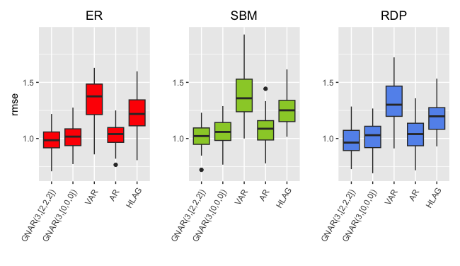
Figure 2: Distribution of RMSE for various time series models ($x$ axis) and network structures (colour), for networks with density approximately 0.1.

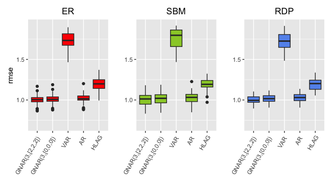
Figure 3: Distribution of RMSE for various time series models ($x$ axis) and network structures (colour), for networks with density approximately 0.4.

The results show that the GNAR-edge(3,[2,2,2]) model, which includes neighbour structure, outperforms all alternative models considered, under all scenarios. In addition, we notice that the performance does not change significantly among the different network structures assumed. The VAR model fitted with the restrict function (VAR) has the worst performance for both networks, with density 0.1 and 0.4. For networks with density 0.1, we are able to fit the VAR model with lag 3, while for networks with density 0.4 this is infeasible due to model complexity; thus, we fit a VAR with lag 1. This simpler model choice may explain the poorer performance of the VAR model for the case of network density 0.4 compared to 0.1. Using the HLAG approach by Nicholson et al., (2020), we are able to fit the VAR model with lag 3 for both networks with density 0.1 and 0.4. We observe that the HLAG estimation yields better predictions compared to the simple VAR case. However, HLAG does not outperform the GNAR-edge model with neighbour structure. Moreover, the AR model which is fitted with lag 3 for all scenarios outperforms the VAR fitted with the HLAG approach in all simulation regimes. Fitting the GNAR-edge model with and without neighbour structure does not lead to considerably different results; however, for the case of density 0.1, the better performance of the GNAR-edge model with neighbour structure is more evident.

Driven by these results, we further explore the effect of different network densities on the predictive performance of the GNAR-edge model with and without neighbour structure. Specifically, for each network structure considered, we simulate 20-node networks with densities ranging from 0.1 to 0.4. For each network density, we simulate 50 graphs and for each simulated graph we further simulate time series of weights for its edges for the same simulation regime considered above. For each resulting network time series, we fit the models GNAR-edge(3,[2,2,2]) and GNAR-edge(3,[0,0,0]) and evaluate their predictive performance by the RMSE. In Appendix A.2, Figures 17(a), 17(b) and 17(c) show the distribution of the RMSE for each network density and network structure. We observe from Figures 17(a), 17(b) and 17(c) that for different network densities, the distribution of the RMSE varies. Notably, we observe an overall better predictive performance of the GNAR-edge model with neighbour structure for smaller densities. As the density increases, the performance of the two GNAR-edge models becomes more similar, echoing our findings from Figures 2 and 3. Nonetheless, in no scenario does the GNAR-edge model with no neighbours outperform the GNAR-edge model with neighbours. These results indicate that sparser networks can be more informative for prediction, but also that different network structures have an effect in the performance, as indicated by the variance of the RMSE for sparser networks.

This finding has triggered our interest in developing a technique for sparsifying the network resulting from the real data, as a potential form of regularization, to possibly assist in predictive performance, as presented in Section 6.

It is also worth noting here that it is anticipated not to see a drastic change in RMSE between the neighbour and no-neighbour assumption, as the data are simulated under the 2-stage neighbour assumption. Increasing the neighbour stages could increase the difference in RMSE between the neighbour and no-neighbour structure, as we see in the next subsection.

5.2.2 Large networks

Next we explore the predictive performance of the models for data that are of similar size to the real data example. First, we consider networks with 86 nodes and network density 0.1 and simulate edge time series with 90 time stamps, for the three different network structures (SBM, ER, RDP). The simulation regime used to generate time series on the edges of the networks is Simulation Regime 1 from Table 3. We repeat each experiment 50 times. In this simulation study, we do not compare to the VAR model as it had poorest performance for moderately sized networks (as seen in Section 5.2.1) even when using the dimensionality reduction approach HLAG. In Appendix A.3, Figure 18 shows the distribution of the RMSE from fitting the different models, for 50 repetitions, on networks with density approximately 0.1. The diameter of the simulated networks is approximately 4. To further mimic the real data sizes, we set up the same experiments for networks with density 0.9, which is close to the network density observed for the real data. As networks with density close to 0.9 are almost complete networks, we perform the experiments only for the ER model. In Appendix A.3, Figure 19 shows the results for networks with density approximately 0.9 and diameter 2.

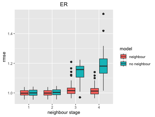
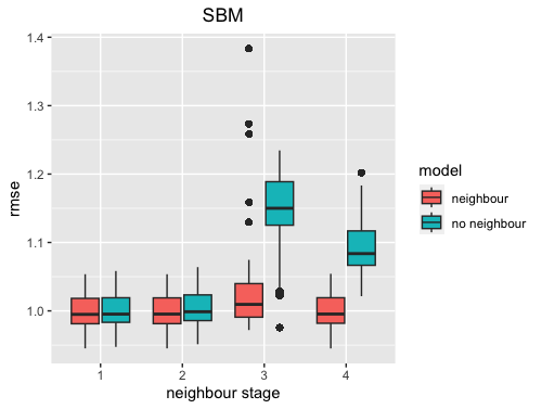
Figure 4: RMSE distribution for GNAR-edge models with and without neighbour structure, for different stages ($x$ axis), on networks with density approximately 0.1. Left: Erdös-Rényi networks; right: Stochastic block model networks.

For this large networks case we obtain similar results to the results obtained from simulations for moderately-sized networks in Section 5.2.1, however, we notice an even poorer performance of the AR model compared to the GNAR-edge model. This can possibly be explained by the increased number of time series to be estimated, which under the AR model are considered individually while the GNAR-edge model analyses them jointly. What is also worth noting is the similar performance of the GNAR-edge models with and without neighbour structure, especially noticeable for the network density 0.9. This can be explained by the simulation regime specified in this experiment, where only 1-stage neighbours are assumed. To illustrate that, we compare the performance of the GNAR-edge model with and without neighbour structure for a range of higher stages. Figure 4 shows the distribution of the RMSE for 50 repetitions of simulation regimes with 1, 2, 3 and 4 stage neighbours. As we do not observe significant changes in performance across the network models considered, we perform these experiments for the ER and SBM structures only. The results suggest that the GNAR-edge model with neighbour structure overall performs better than models with no neighbour structure for networks with a more complex topology, and higher stage neighbours.

5.3 Model misspecification

In this section, we investigate the performance of the GNAR-edge model in estimation and prediction, under model misspecification scenarios. Specifically, we consider three alternative types of model misspecification. First, we explore the estimation and predictive performance of the model for simulated network time series with heavy-tailed noise, and specifically we consider a t-distribution with 3 and 10 degrees of freedom (chosen to ensure that the distribution has finite variance). Second, we examine the estimation performance of the GNAR-edge model in settings where innovations are correlated across time. Third, we explore the model performance under misspecification of the network connectivity patterns. For each case, we consider both moderately-sized and large networks.

5.3.1 Moderately-sized networks

For moderately sized networks, we consider the simulated data of Section 5.1.1, and specifically the $4^{th}$ simulation regime presented in Table 1 as this is the most complex regime with respect to the number of parameters to be estimated. We simulate 20-node networks and time series on the edges of the networks under the GNAR-edge model with parameters as per simulation regime 4 in Table 1, while the innovations are simulated from a heavy-tailed distribution. Notably, we consider a t-distribution with two different parameter specifications that control the probability mass in the tails of the distribution. First we consider a more heavy-tailed case assuming 3 degrees of freedom, and second we consider a less heavy-tailed case assuming 10 degrees of freedom. We perform 50 repetitions of each experiment and report the absolute error between the estimated coefficients and their true values. Figure 5 shows the distribution of the absolute error for all autoregressive parameters, under normally distributed (n) and t-distributed with 3 degrees of freedom (t) innovations, for different network structures. The results for the stage-1 and stage-2 neighbour effect parameters are similar to the results presented for the autoregressive parameters, thus they are presented in Appendix A.4, Figures 20 and 21.

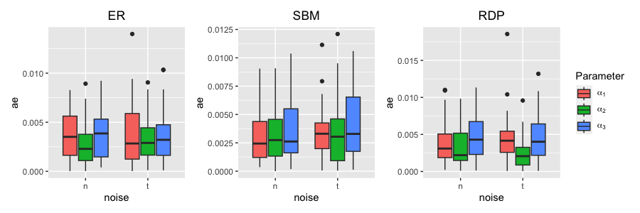
Figure 5: Distribution of absolute error for autoregressive parameters $\alpha_{1},\alpha_{2},\alpha_{3}$, for different network structures, and normally distributed (n) and t-distributed with 3 degrees of freedom (t) innovations.

The estimation performance of the GNAR-edge model on simulated data with t-distributed innovations is similar to that with normally distributed innovations. However, we notice that for the autoregressive parameters, the distribution of the absolute error has more outliers for the heavy-tailed case compared to the normally distributed innovations. Despite the overall similar estimation performance for the two different innovation distributions, we anticipate that the prediction performance will be poorer for the synthetic data with heavy-tailed innovations. We investigate that by evaluating the predictive performance of the GNAR-edge model on the synthetic data with normally distributed and heavy-tailed innovations, for the same simulation regime. To do that we fit the GNAR-edge model to the network time series excluding the last time stamp, use the fitted model to predict the last time stamp and evaluate the prediction performance using the RMSE. The boxplots in Figure 6 show the distribution of the RMSE for 50 repetitions of the experiment. As expected, the RMSE obtained for the heavier-tailed network time series is bigger compared to the case of normally distributed errors. In Appendix A.4 we also present the results from experiments for t-distributed innovations with 10 degrees of freedom, for which we observe a similar estimation performance to that of 3 degrees of freedom, and a slightly better predictive performance as the innovations are less heavy-tailed for degrees of freedom 10.

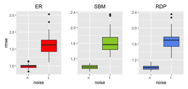
Figure 6: Distribution of RMSE for normally distributed (n) and t-distributed with 3 degrees of freedom (t) innovations, for different network structures.

We now examine the model performance in settings where the innovations of the network time series are correlated across time. In this simulation scenario, we simulate network time series with innovations coming from a multivariate normal distribution with mean 0 and variance 1, for two different correlation sizes among all pairs of normally distributed variables equal to 0.1 and 0.5, for less and more strongly correlated innovations respectively. Similarly to previous experiments, we consider the $4^{th}$ simulation regime to generate the network time series under the GNAR-edge model with correlated errors, and fit the GNAR-edge model to the simulated data, for 50 repetitions. First we present the results for correlation equal to 0.5. In Figure 7, we present the distribution of the absolute error for the estimated model parameters across the 50 repetitions for the SBM network structure, for correlated and independent innovations. Similar results are obtained for the ER and RDP network structures, thus they are presented in Appendix A.4, Figures 26 and 27.

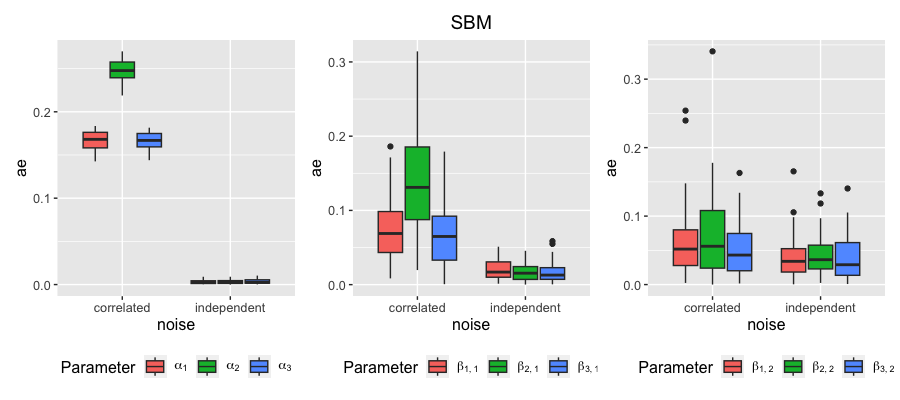
Figure 7: Distribution of absolute error for all model parameters for settings with independent and correlated innovations with correlation 0.5, for SBM network structure.

The estimation performance of the GNAR-edge model changes to a different extent for the different model parameters. For the autoregressive parameters, in Figure 7 we see a clear effect of the correlated errors on the estimation performance against the independent errors case, with the estimation performance for the former being considerably poorer. The colours are not distinguishable for the autoregressive parameters in the independent errors setting in Figure 7, due to the large difference in the scale of the absolute error in the correlated errors setting.) For a closer look to the distributions of the absolute error for the autoregressive parameters in the independent noise setting see Figure 5, middle plot, (n) case. For the 1-stage neighbour effect parameters, we see again that the estimation performance of the GNAR-edge is poorer for the correlated innovations case, however, the scale of the absolute error is now smaller compared to the scale of the absolute error for the autoregressive parameters. Similarly for the 2-stage neighbour effect, we notice an even smaller scale of the absolute error for the correlated innovations, however the estimation performance is still poorer compared to the independent innovations. This is a reasonable finding given that the dependence of the errors is introduced across time, rather than across the edges of the network, thus having a stronger effect on the autoregressive parameters compared to the network effect parameters. Overall, we observe that the estimation performance of the GNAR-edge model is poorer for all model parameters when innovations are correlated across time, as anticipated.

We repeat the above experiments for correlation equal to 0.1 and present the results in Appendix A.4. We observe a similar performance of the GNAR-edge model for 0.1 correlation to that of 0.5 correlation among innovations; however, the scale of the absolute error in this setting is smaller, due to the smaller correlation introduced.

We also investigate the estimation performance of the GNAR-edge model under misspecification of the neighbourhood structure, for the same simulation regime, as follows. After simulating the network time series, we perform edge rewiring for different rewiring probabilities using the rewire function from the R package igraph, and fit the GNAR-edge model to the data using the rewired network. We specify the rewiring method each$\_$edge within the rewire function that rewires the endpoints of edges with a constant probability uniformly at random to a new node in the graph. In our experiments, we consider rewiring probabilities of 0.05, 0.1, 0.15 and 0.2. Each of these rewiring probabilities correspond to an approximate change of 25, 45, 65 and 80 edges, respectively, in the original network with 380 possible edges. We perform 50 repetitions and report the RMSE of the estimated coefficients with respect to their true values. Figure 8 shows how the RMSE scales for increasing rewiring probabilities. The mean Hamming distance between the rewired networks and corresponding true networks among the 50 repetitions is 0.067, 0.12, 0.17 and 0.21, respectively for each rewiring probability 0.05, 0.1, 0.15 and 0.2, indicatively for the ER network structure. Similar sizes of mean Hamming distance are obtained for the SBM and RDP networks.

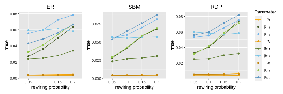
Figure 8: RMSE of estimated model parameters after 50 repetitions, and various perturbations of network structure (x axis).

The RMSE for the network effect parameters increases for increasing perturbations of the network structure, as it would be anticipated. Specifically, we observe a more drastic increase of the RMSE for the network effect parameters for lag $L=1,3$, while for the autoregressive parameters and the the network effect parameters for lag $L=2$, we observe a more stable RMSE. This is especially anticipated for the autoregressive parameters as they are not capturing network information.

5.3.2 Large networks

In this section, we repeat the same simulation experiments for our model misspecification settings, for large networks. Specifically, we consider 86-node networks and simulate network time series under simulation regime 1 of Table 3. Similarly to moderately-sized network in the previous section, we first explore the estimation performance of the GNAR-edge model for heavy-tailed innovations. For the large networks setting, we consider only the case of t-distribution with 3 degrees of freedom as this is the heavier-tailed case, and for moderately-sized networks we did not observe considerably different results between 3 and 10 degrees of freedom. The results of the simulation experiments are presented in Appendix A.5, in Figures 31, 32 and 33, which show the distribution of the absolute error of the estimated parameters and the RMSE of the predictions, under normally distributed and t-distributed innovations, for different network structures. Similarly to results of the previous section, we notice that the estimation performance of the GNAR-edge model is similar in both settings of correlated and independent innovations, while, as seen in Figure 33 the prediction performance of the GNAR-edge model is considerably worse in the case of heavy-tailed network time series, as anticipated.

We also examine the effect of time correlated innovations for large networks. Similarly to our experiments for moderately-sized networks, we simulate edge time series for large networks, under two scenarios, (i) with i.i.d. innovations simulated from a standard normal distribution and (ii) with innovations simulated from multivariate standard normal distribution with correlation 0.5 across variables. In this experiments we consider only the 0.5 correlation scenario, as it is the setting that had the greatest effect in the estimation performance for moderately-sized networks, as seen in Section 5.3.1. We perform again 50 repetitions and present the results for the estimation performance of the GNAR-edge model in Figure 9 for the SBM network structure. The results for the ER and RDP networks are presented in Appendix A.5, Figures 34 and 35.

Figure 9: Distribution of absolute error for all model parameters for settings with independent and correlated innovations with correlation 0.5, for SBM network structure.

Figure 9, left panel, shows only the distribution of the absolute error for the correlated errors setting as colours would not be distinguishable if results were included in the same plot for the independent errors setting, due to the difference in the scale of the absolute error. For the results in the independent error case see Figures 31, 32 (n) case. Similarly to the moderately-sized networks, we observe that the estimation performance of the GNAR-edge model is considerably poorer for the correlated innovations setting, particularly notable for the autoregressive parameters of the model as seen in Figure 9 left panel and Figure 31 middle panel (n) case.

We further explore the estimation performance of the GNAR-edge model under misspecification of the neighbourhood structure, in the large networks setting. We rewire the edges of the true network with rewiring probabilities 0.05, 0.1, 0.15 and 0.2, which correspond to an approximate change of 139, 270, 395 and 512 edges, respectively, in the original network with 7310 possible edges. We perform 50 repetitions and report the RMSE of the estimated parameters in Figure 36. The mean Hamming distance between the rewired networks and corresponding true networks among the 50 repetitions is 0.018, 0.037, 0.054 and 0.07, respectively for each rewiring probability, indicatively for the ER network structure, with similar sizes of mean Hamming distance obtained for the SBM and RDP networks.

Similarly to moderately-sized networks, we notice that the estimation of the autoregressive parameters is not affected by the perturbed networks, however, the estimated parameters for the network effect move further away from their true values as the rewiring probability increases. Nonetheless, for the network effect parameters at lag $l=2,4$, and especially for the network effect parameter at lag $l=4$, $\beta_{4,1}$, the effect of the network misspecification for increasing rewiring probability is relatively more stable.

6 Real data application

In this section, we consider the multivariate time series data set described in Section 2 resulting from anonymised and aggregated transactions between 2-digit SIC codes, ranging from January 2015 to July 2022. The network emerging from the pairwise transactions comprises of 90 nodes (2-digit SIC) and 7,152 directed edges (transactions), being a very densely connected network with density approximately 0.9. Our simulations have shown that sparser networks can assist in better prediction performance. Thus, here we propose a technique for sparsifying networks arising from multivariate time series.

6.1 Network sparsification

Our technique is based on lead-lag analysis. The investigation of leading and lagging relationships between time series is a common approach for analysing multivariate time series systems Wu et al., (2010). A time series A is said to lead a time series B if past values of time series A are more strongly correlated with future values of time series B than with past values of time series B. Thus, lead-lag analysis can be very informative for forecasting. To investigate such relationships between multiple time series, pairwise distances of the time series with respect to a lead-lag metric can be employed. This results in a lead-lag matrix with rows and columns corresponding to each individual time series. Bennett et al., (2022) present a range of alternatives for specifying a lead-lag metric. In our study, we investigate the lead-lag relationships among the observed multiple time series of transactions, specifying Pearson’s correlation and considering the difference of the cross-correlation function at lag $\in\left\{-1,1\right\}$ (ccf-lag1 as presented in Bennett et al., (2022)).

Using the lead-lag analysis, we sparsify the network by identifying the top leading edges. To this end, we consider the row sums of the lead-lag matrix, which we take as indicator of the size of leadingness of each time series over the rest of the time series. We consider the top 801 leading edges in the network, resulting in a network with density 0.1, which is the setting for which the smallest RMSE has been achieved in simulations.

As a check of the network choice, we assess whether the resulting network has small-world structure, a characteristic of many real networks; in particular, de la Torre et al., (2016) study an economic network of transactions in Estonia, and they observe that it is characterised by small-world behaviour. The two network properties that indicate small-world behaviour are an average shortest path length of similar size as that of a Bernoulli random graph with same network density, (often) coupled with an average local clustering coefficient which is high compared to that of a corresponding Bernoulli random graph. Our resulting network has an average local clustering coefficient 0.2, which is considerably larger than the expected clustering coefficient of 0.1 for a 90-node random graph with 0.1 density. However, the average shortest path length is 2.3, which is only slightly higher than the expected average shortest path length of 2 for a random 90-node graph with 0.1 density. These results taken together hint at the possible presence of a small-world structure in our sparsified network.

6.2 Predictive performance

After sparsifying the network, we consider as training sample the time series observed on the edges of the network up to June 2022. We pre-process the time series by carrying out first-order differencing to remove trend, and by dividing by the standard deviation for each edge of the training sample to reduce heterogeneity. We fit the GNAR-edge model to the training data and predict the last time stamp, July 2022. The predictive performance is again evaluated using the RMSE over all the time series. We examine the predictive performance for a range of lags $l=\{1,\ldots,9\}$ and neighbour stages $r=\{0,1,2,3,4\}$ and present the results in Figure 10.

Figure 10 shows that increasing the lag size leads to better prediction performance, as revealed by the decreasing RMSE. Notably, we observe a steep decrease of the RMSE up to lag 3, beyond which the RMSE gradually decreases until it achieves a (possibly local) minimum at lag 8. We further observe similar predictive performance up to and including lag 2 for all different neighbour stages considered for the GNAR-edge model, while after lag 2, the performance of the alternative models starts to vary. In addition, 1-stage and 2-stage neighbour models have similar predictive performance across lags as seen by the overlapping lines. However, for lag 8 when the RMSE is minimised, the 1-stage neighbour model has the best performance among the models, with the remaining models having very similar RMSEs.

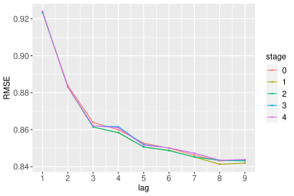
Figure 10: RMSE from predicting the last time stamp of the time series, for various lags ($x$ axis) and neighbour stages (colour).

We compare these results to the results from fitting an AR model, the model class which has shown the most competitive performance to our GNAR-edge models in our synthetic data experiments. The results in Figure 10 showcase that the best performing model is the GNAR-edge model for lag 8 and 1-stage neighbours. In light of this, we fit an AR(8) model to the time series resulting after network sparsification and predict the last time stamp, which yields an RMSE of 0.9433. This RMSE is considerably higher than the RMSE obtained from the GNAR-edge model with lag 8 and 1-stage neighbours, being 0.8412. In the Supplementary Material, Section 2, we present the results from fitting an AR model for a range of lags from 1 up to 7, all of which attain an RMSE very close to the RMSE obtained from fitting an AR(8) model. To further illuminate the utility of the sparsification step in improving the prediction performance of our model, we consider the whole network, and fit the GNAR-edge model with lag 8 and 1-stage neighbours. The RMSE obtained when considering the whole network is 1.3864, which is considerably larger than the RMSE of 0.8412, obtained for the sparsified network.

From Figure 10, we notice that for each lag, there is no considerable variability in the scale of the RMSE across the different stages of neighbours. This can perhaps be explained by the fact that the best fitting model as suggested by the results, is the model with 1-stage neighbours, and as seen in synthetic data experiments for 1-stage neighbours we do not observe considerable changes in the RMSE versus the case with no neighbours assumed. Figure 11 illustrates the fit of the GNAR-edge model with lag 8 and 1-stage neighbours, indicatively for two of the 801 edge time series. We observe an overall very good fit of the GNAR-edge model on the real data; however, larger peaks of the time series are not fully captured by the model.

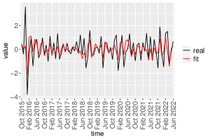
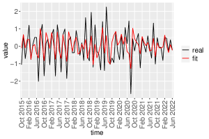
Figure 11: Fitted lines (red) on two real time series (black) from fitting a GNAR-edge model with lag 8 and 1-stage neighbours on the sparsified network.

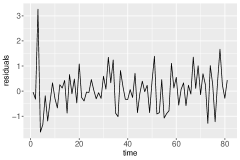
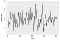
Figure 12: Residuals for plotted time series from fitting GNAR-edge model on the sparsified network.

6.3 Assessing model fit

To assess model fit, we next investigate the residuals from fitting the model on the sparsified network. In Figure 12, we further plot the residuals for the edge time series of Figure 11, respectively. In Figure 12, we further plot the residuals for the edge time series of Figure 11, respectively. A challenge with performing a full residual analysis is that we have multiple (801) time series. Thus, we first consider an approach for summarising the residuals across the multiple time series. First, we plot the distribution of the residuals across the time series for each time stamp, shown in Figure 13. We observe that overall, residuals are distributed around 0, however, there are several outliers. We further consider the mean residual across the edge time series, for each time stamp, and plot the histogram, line, quantile-quantile plot and autocorrelation of the resulting mean residuals as shown in Figure 14. The plots suggest that the mean residuals could be modelled as normally distributed around 0, as also suggested by the Shapiro-Wilk normality test with $p$-value=0.78.

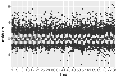
Figure 13: Distribution of residuals across time series for each time stamp ($x$ axis).

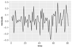
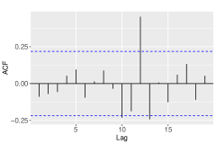
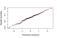
Figure 14: Mean residuals from fitting the GNAR-edge model on the sparsified network.

Lastly, we plot the fitted values versus the residuals in Figure 15, with colours corresponding to different years. The side plots in Figure 15 show the marginal distributions for the different years. In view of the model assuming that the errors come from independent standard multivariate normal distributions, it is thus encouraging to see that the marginal distribution exhibit a close to normal shape, as well as that there is not a specific pattern followed by the residuals across time.

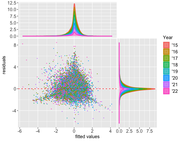
Figure 15: Fitted values (x axis) versus residuals (y axis) among multiple time series with points with same colour corresponding to year, for multiple time series.

7 Conclusion

In this paper, we introduce a generalised network autoregressive model for networks with time varying edge weights, which we dub as the GNAR-edge model. The GNAR-edge model exploits the underlying network structure of multivariate time series observed on the edges of the network. Synthetic data experiments validate the performance of the GNAR-edge model in parameter estimation and prediction. Comparisons to baseline models used for the analysis of multivariate time series systems show that the GNAR-edge model can improve predictions when there is an underlying network structure in the data.

The GNAR-edge model is motivated by an anonymised and aggregated UK business payments data set made available to the Office for National Statistics by Pay.UK and Vocalink, which can be represented as a graph with time varying edge weights. The real network is a very densely connected network and thus we propose an approach for sparsifying the network using a lead-lag analysis of the time series. Results show that the GNAR-edge model offers considerably more accurate predictions for the real data versus baseline models, especially after network sparsification.

An avenue for future work would be the investigation of communities formed by the edges of the network, and the inclusion of community structure information in the autoregressive model. In the network literature, there is vast research on the topic of identifying communities formed by the nodes of the network. On the other hand, the topic of communities formed by the edges of the network has attracted relatively less attention (see Suveges and Olhede, (2023) and references therein). As in our example edges are associated with time series, a viable theoretically-grounded approach to recover the underlying edge communities is to investigate the lead-lag relationships of the time series. Specifically, as introduced in Bennett et al., (2022), one can construct a lead-lag network from leading and lagging relationships between time series, and subsequently perform node clustering, which corresponds to time series clustering. One way to use the information from edge time series clustering is to incorporate it in the GNAR-edge model through weights in (4), under the assumption that edges belonging to the same cluster have a greater effect on each other compared to edges belonging to different clusters.

Another interesting extension of our model would be the inclusion of node and edge covariates. Information on the nodes or the edges of a graph is commonly available in many real network applications. Incorporating such information in the model in the form of covariates may enhance the prediction performance.

Furthermore, in the GNAR-edge model, the network effect is encoded by a single parameter, for both incoming and outgoing neighbouring edges, for each edge. In certain applications, it might be of interest to encode the effect of incoming and outgoing edges separately, through two different parameters. This can be especially relevant to financial applications, and specifically payments data, where a payment from $i$ to $j$ may depend on payments received by $i$ and payments made by $i$ in a different way. This distinction could be introduced in the GNAR-edge and explored as future work.

Computing

All experiments were run on MacBook Pro M1 machine.

Funding

The authors gratefully acknowledge the ONS-Turing Strategic partnership for funding. Gesine Reinert was supported in part by the Engineering and Physical Sciences Research Council (EPSRC) grants [EP/T018445/1, EP/R018472/1, EP/X0021951].

Appendix A Appendix: Additional results for the synthetic data experiments

A.1 Some network illustrations

In Figure 16, we present a network instance for each network structure considered (ER, SBM, RDP) for synthetic data experiments of Section 5.1.1.

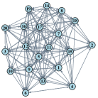
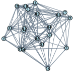
Figure 16: A simulated ER network (left), SBM network (middle) and RDP network (right), for each of which time series on the edges are simulated.

A.2 The effect of network density on the predictive performance for moderately-sized networks

In Figure 17 we report the results obtained from investigating the predictive performance of the GNAR-edge model with and without network structure, for different network densities, as discussed in Section 5.2.1.

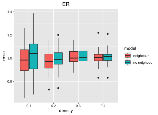
(a) Distribution of RMSE for various network densities ($x$ axis) and GNAR-edge model with and without neighbour structure, for Erdös-Rényi networks.

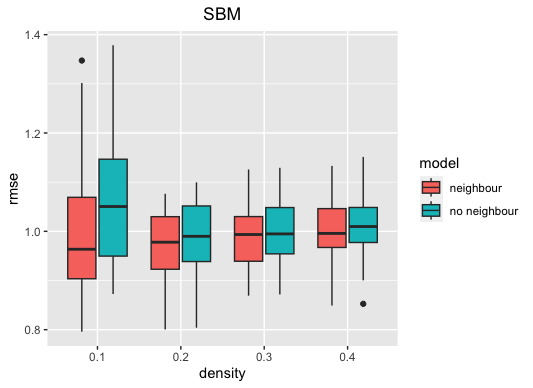
(b) Distribution of RMSE for various network densities ($x$ axis) and GNAR-edge model with and without neighbour structure, for SBM networks.

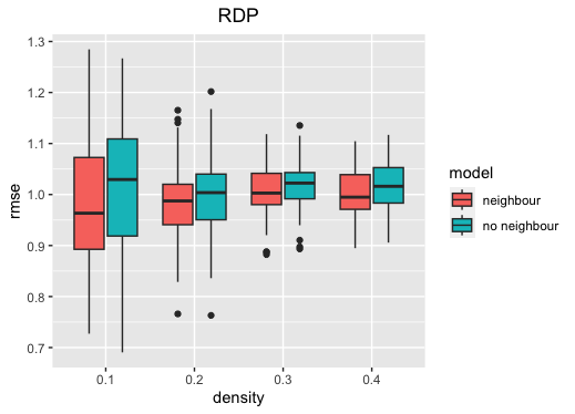
(c) Distribution of RMSE for various network densities ($x$ axis) and GNAR-edge model with and without neighbour structure, for RDP networks.

Figure 17: Distribution of RMSE for various network densities ($x$ axis) and network structures (subfigures), after fitting the GNAR-edge model with and without neighbour structure.

A.3 Comparisons of predictive performance for large networks

In this section, Figures 18 and 19 show results from comparing the predictive performance of the GNAR-edge model and a simple AR model, for large networks, as discussed in Section 5.2.2.

Figure 18: Distribution of RMSE for different structures Erdös-Rényi, SBM and RDP, for 86-node networks with density approximately 0.1.

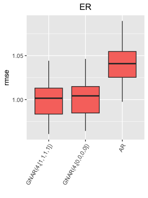
Figure 19: Distribution of RMSE for Erdös-Rényi network structure, for 86-node networks with density approximately 0.9.

A.4 Additional results for model misspecification for moderately-sized networks

In this section we present the results for the estimation and predictive performance of the GNAR-edge model under different model misspecification scenarios.

First, Figures 20 and 21 show the distribution of the absolute error of the estimated parameters for the network effect, considering normally distributed innovations (n) and t-distributed innovations with 3 degrees of freedom (t), as discussed in Section 5.3.1.

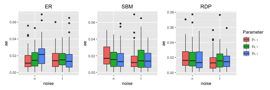
Figure 20: Distribution of absolute error for network effect parameters $\beta_{1,1},\beta_{2,1},\beta_{3,1}$, for different network structures, and normally distributed (n) and t-distributed with 3 degrees of freedom (t) innovations.

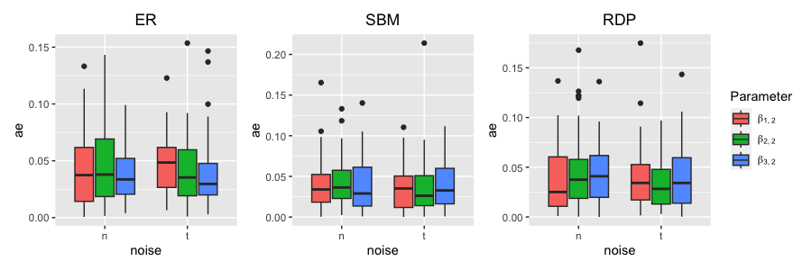
Figure 21: Distribution of absolute error for network effect parameters $\beta_{1,2},\beta_{2,2},\beta_{3,2}$, for different network structures, and normally distributed (n) and t-distributed with 3 degrees of freedom (t) innovations.

Similarly Figures 22, 23, 24 and 25 show the estimation and prediction performance for network time series simulated with normally distributed and t-distributed innovations with 10 degrees of freedom.

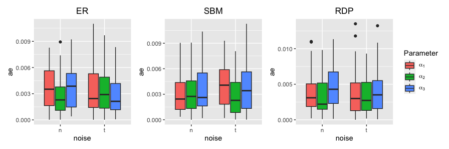
Figure 22: Distribution of absolute error for autoregressive parameters $\alpha_{1},\alpha_{2},\alpha_{3}$, for different network structures, and normally distributed (n) and t-distributed with 10 degrees of freedom (t) innovations.

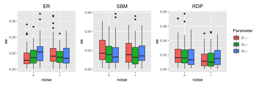
Figure 23: Distribution of absolute error for network effect parameters $\beta_{1,1},\beta_{2,1},\beta_{3,1}$, for different network structures, and normally distributed (n) and t-distributed with 10 degrees of freedom (t) innovations.

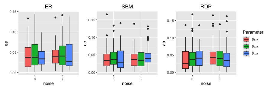
Figure 24: Distribution of absolute error for network effect parameters $\beta_{1,2},\beta_{2,2},\beta_{3,2}$, for different network structures, and normally distributed (n) and t-distributed with 10 degrees of freedom (t) innovations.

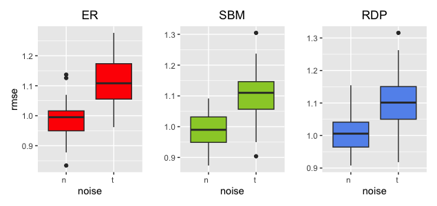
Figure 25: Distribution of RMSE for normally distributed (n) and t-distributed with 10 degrees of freedom (t) innovations, for different network structures.

In Figures 26 and 27, we present the results for the estimation performance of the GNAR-edge model for i.i.d. innovations generated from multivariate standard normal distribution and correlated innovations generated from multivariate standard normal distribution with correlation 0.5, for ER and RDP networks, as discussed in Section 5.3.1.

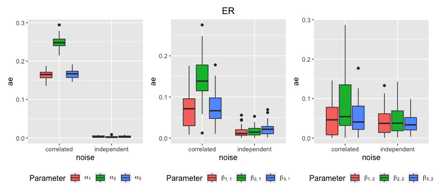
Figure 26: Distribution of absolute error for all model parameters for settings with independent and correlated innovations with correlation 0.5, for ER network structure.

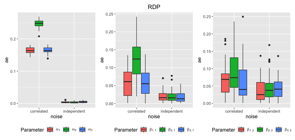
Figure 27: Distribution of absolute error for all model parameters for settings with independent and correlated innovations with correlation 0.5, for RDP network structure.

We further perform the same experiments for independent and correlated innovations with correlation 0.1, as discussed in Section 5.3.1. The estimation performance of the GNAR-edge model is presented in Figures 28, 29 and 30.

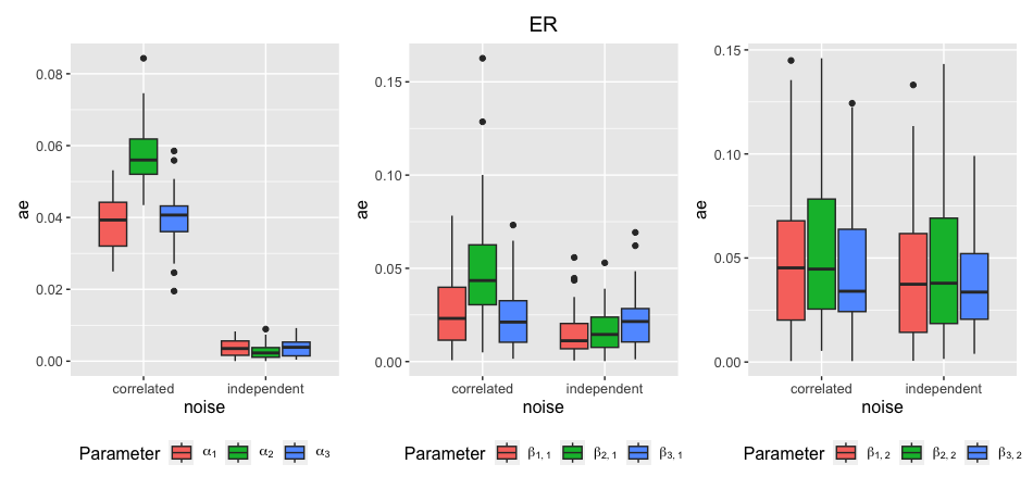
Figure 28: Distribution of absolute error for all model parameters for settings with independent and correlated innovations with correlation 0.1, for ER network structure.

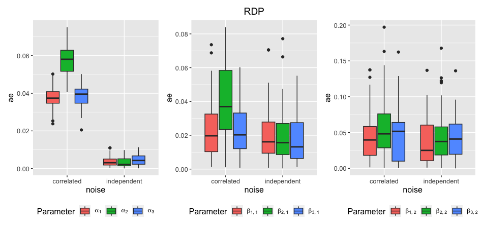
Figure 29: Distribution of absolute error for all model parameters for settings with independent and correlated innovations with correlation 0.1, for RDP network structure.

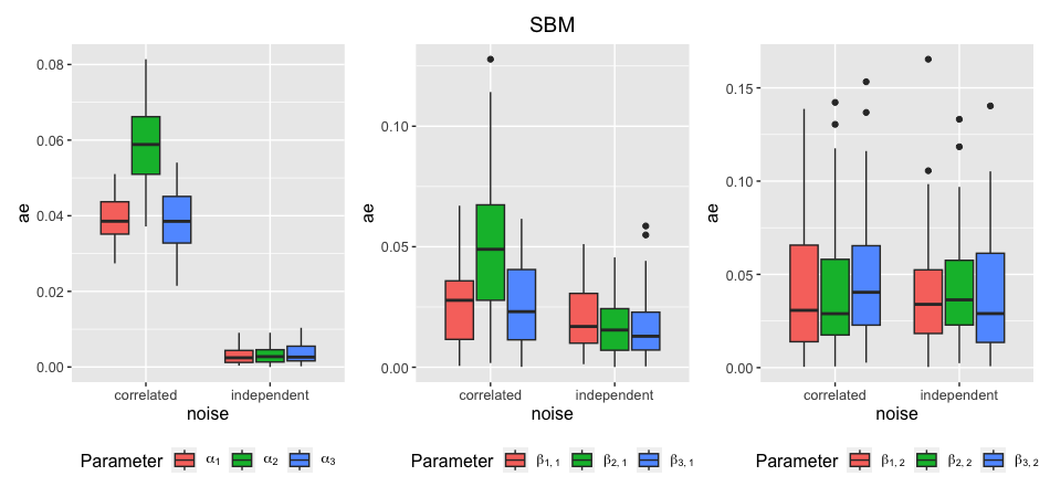
Figure 30: Distribution of absolute error for all model parameters for settings with independent and correlated innovations with correlation 0.1, for SBM network structure.

A.5 Additional results for model misspecification for large networks

In this section we present results for synthetic data experiments performed under model misspecification settings for large networks, as discussed in Section 5.3.2.

Figures 31 and 32 show the distribution of the absolute error of the estimated parameters, for synthetic data generated with normally distributed and t-distributed innovations with 3 degrees of freedom, for all network structures considered. Figure 33 shows the distribution of the RMSE for predicting the last time stamp, under normally distributed and t-distributed innovations with 3 degrees of freedom.

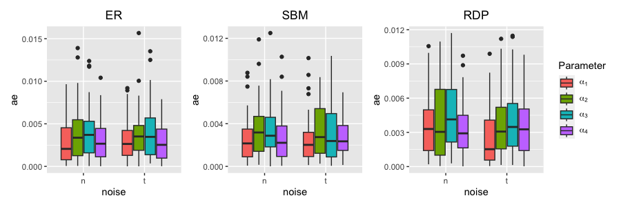
Figure 31: Distribution of absolute error for autoregressive parameters $\alpha_{1},\alpha_{2},\alpha_{3},\alpha_{4}$, for different network structures, and normally distributed (n) and t-distributed with 3 degrees of freedom (t) innovations.

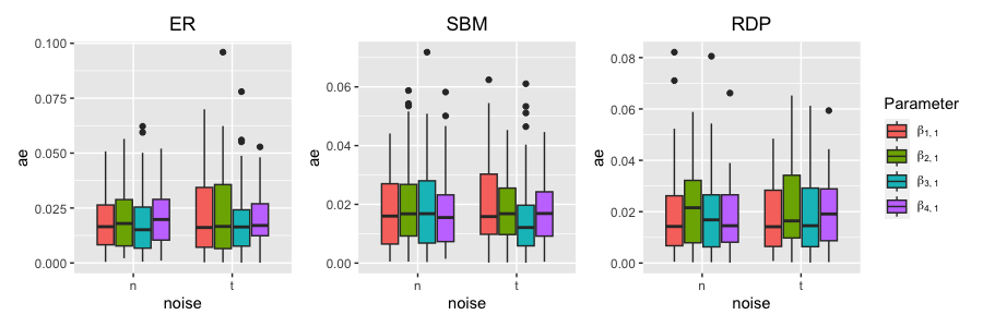
Figure 32: Distribution of absolute error for network effect parameters $\beta_{1,1},\beta_{2,1},\beta_{3,1},\beta_{4,1}$, for different network structures, and normally distributed (n) and t-distributed with 3 degrees of freedom (t) innovations.

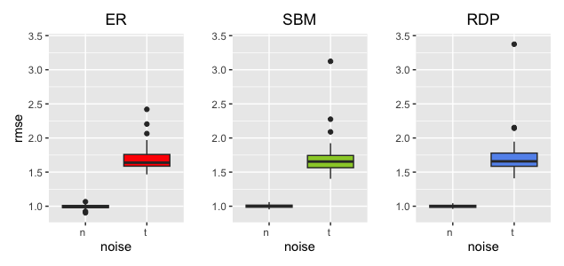
Figure 33: Distribution of RMSE for normally distributed (n) and t-distributed with 3 degrees of freedom (t) innovations, for different network structures.

Figures 34 and 35 show the estimation performance of the GNAR-edge model for independent and correlated innovations with correlation 0.5, for ER and RDP network structures. Figures 34 and 35, left panels, show only the distribution of the absolute error for the correlated errors setting as colours are indistinguishable when independent errors setting is included in same plot, due to difference in the scale of the absolute error. For the results for the autoregressive parameters under the independent errors setting, see Figures 31, 32 (n) case.

Figure 34: Distribution of absolute error for all model parameters for settings with independent and correlated innovations with correlation 0.5, for ER network structure.

Figure 35: Distribution of absolute error for all model parameters for settings with independent and correlated innovations with correlation 0.5, for RDP network structure.

Figure 36 shows the RMSE for all mdoel parameters and network structures under misspecification of the network structure through edge rewiring, for different rewiring probabilities.

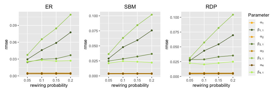
Figure 36: RMSE of estimated model parameters after 50 repetitions, and various perturbations of network structure (x axis).

References

- Abdi and Amrit, (2021) Abdi, A. and Amrit, C. (2021). A review of travel and arrival-time prediction methods on road networks: classification, challenges and opportunities. PeerJ Computer Science, 7:e689.
- Armillotta and Fokianos, (2021) Armillotta, M. and Fokianos, K. (2021). Poisson network autoregression. arXiv preprint arXiv:2104.06296.
- Bennett et al., (2022) Bennett, S., Cucuringu, M., and Reinert, G. (2022). Lead–lag detection and network clustering for multivariate time series with an application to the us equity market. Machine Learning, pages 1–42.
- Bernanke et al., (2005) Bernanke, B. S., Boivin, J., and Eliasz, P. (2005). Measuring the effects of monetary policy: a factor-augmented vector autoregressive (favar) approach. The Quarterly Journal of Economics, 120(1):387–422.
- Box et al., (2015) Box, G. E., Jenkins, G. M., Reinsel, G. C., and Ljung, G. M. (2015). Time Series Analysis: Forecasting and Control. John Wiley & Sons.
- Buda et al., (2022) Buda, G., Hansen, S., Rodrigo, T., Carvalho, V., Ortiz, Á., and Mora, J. V. R. (2022). National accounts in a world of naturally occurring data: A proof of concept for consumption. Cambridge Working Papers, Faculty of Economics, University of Cambridge.
- Carvalho et al., (2021) Carvalho, V. M., Garcia, J. R., Hansen, S., Ortiz, Á., Rodrigo, T., Rodríguez Mora, J. V., and Ruiz, P. (2021). Tracking the covid-19 crisis with high-resolution transaction data. Royal Society Open Science, 8(8):210218.
- Chen et al., (2023) Chen, E. Y., Fan, J., and Zhu, X. (2023). Community network auto-regression for high-dimensional time series. Journal of Econometrics, 235(2):1239–1256.
- Companies House, (2018) Companies House, U. K. (2018). Standard industrial classification of economic activities (SIC). https://www.gov.uk/government/publications/standard-industrial-classification-of-economic-activities-sic.
- Csardi and Nepusz, (2006) Csardi, G. and Nepusz, T. (2006). The igraph software package for complex network research. InterJournal, Complex Systems:1695.
- Dallakyan et al., (2022) Dallakyan, A., Kim, R., and Pourahmadi, M. (2022). Time series graphical lasso and sparse var estimation. Computational Statistics & Data Analysis, 176:107557.
- Davis et al., (2016) Davis, R. A., Zang, P., and Zheng, T. (2016). Sparse vector autoregressive modeling. Journal of Computational and Graphical Statistics, 25(4):1077–1096.
- de la Torre et al., (2016) de la Torre, S. R., Kalda, J., Kitt, R., and Engelbrecht, J. (2016). On the topologic structure of economic complex networks: empirical evidence from large scale payment network of Estonia. Chaos, Solitons & Fractals, 90:18–27.
- Durante and Dunson, (2016) Durante, D. and Dunson, D. B. (2016). Locally adaptive dynamic networks. The Annals of Applied Statistics, 10(4):2203–2232.
- Fu et al., (2009) Fu, W., Song, L., and Xing, E. P. (2009). Dynamic mixed membership blockmodel for evolving networks. In Proceedings of the 26th annual International Conference on Machine Learning, pages 329–336.
- Hanneke et al., (2010) Hanneke, S., Fu, W., and Xing, E. P. (2010). Discrete temporal models of social networks. Electronic Journal of Statistics, 4:585–605.
- Jiang et al., (2020) Jiang, B., Li, J., and Yao, Q. (2020). Autoregressive networks. arXiv preprint arXiv:2010.04492.
- Kang et al., (2021) Kang, X., Ganguly, A., and Kolaczyk, E. D. (2021). Dynamic networks with multi-scale temporal structure. Sankhya A, pages 1–43.
- Knight et al., (2020) Knight, M., Leeming, K., Nason, G., and Nunes, M. (2020). Generalised network autoregressive processes and the GNAR package. Journal of Statistical Software, 96(5):1–36.
- Koop, (2013) Koop, G. M. (2013). Forecasting with medium and large bayesian vars. Journal of Applied Econometrics, 28(2):177–203.
- Krivitsky and Handcock, (2014) Krivitsky, P. N. and Handcock, M. S. (2014). A separable model for dynamic networks. Journal of the Royal Statistical Society. Series B, Statistical Methodology, 76(1):29.
- Ludkin et al., (2018) Ludkin, M., Eckley, I., and Neal, P. (2018). Dynamic stochastic block models: parameter estimation and detection of changes in community structure. Statistics and Computing, 28:1201–1213.
- Lütkepohl, (2005) Lütkepohl, H. (2005). New introduction to multiple time series analysis. Springer Science & Business Media.
- Matias and Miele, (2017) Matias, C. and Miele, V. (2017). Statistical clustering of temporal networks through a dynamic stochastic block model. Journal of the Royal Statistical Society. Series B (Statistical Methodology), 79(4):1119–1141.
- Menelaou et al., (2018) Menelaou, C., Kolios, P., Timotheou, S., and Panayiotou, C. G. (2018). Effective prediction of road segment occupancy for the route-reservation architecture. IFAC-PapersOnLine, 51(9):470–475.
- Min and Wynter, (2011) Min, W. and Wynter, L. (2011). Real-time road traffic prediction with spatio-temporal correlations. Transportation Research Part C: Emerging Technologies, 19(4):606–616.
- Nicholson et al., (2020) Nicholson, W. B., Wilms, I., Bien, J., and Matteson, D. S. (2020). High dimensional forecasting via interpretable vector autoregression. The Journal of Machine Learning Research, 21(1):6690–6741.
- Pensky, (2019) Pensky, M. (2019). Dynamic network models and graphon estimation. The Annals of Statistics, 47(4):2378–2403.
- Salamanis et al., (2015) Salamanis, A., Kehagias, D. D., Filelis-Papadopoulos, C. K., Tzovaras, D., and Gravvanis, G. A. (2015). Managing spatial graph dependencies in large volumes of traffic data for travel-time prediction. IEEE Transactions on Intelligent Transportation Systems, 17(6):1678–1687.
- Sarkar and Moore, (2005) Sarkar, P. and Moore, A. W. (2005). Dynamic social network analysis using latent space models. ACM SIGKDD Explorations Newsletter, 7(2):31–40.
- Sioofy Khoojine et al., (2021) Sioofy Khoojine, A., Shadabfar, M., Hosseini, V. R., and Kordestani, H. (2021). Network autoregressive model for the prediction of covid-19 considering the disease interaction in neighboring countries. Entropy, 23(10):1267.
- Spencer et al., (2015) Spencer, S. E., Hill, S. M., and Mukherjee, S. (2015). Inferring network structure from interventional time-course experiments. The Annals of Applied Statistics, 9(1):507–524.
- Suveges and Olhede, (2023) Suveges, M. and Olhede, S. C. (2023). Networks with correlated edge processes. Journal of the Royal Statistical Society Series A: Statistics in Society, 186:441–462.
- Tsay, (2013) Tsay, R. S. (2013). Multivariate time series analysis: with R and financial applications. John Wiley & Sons.
- Wu et al., (2010) Wu, D., Ke, Y., Yu, J. X., Yu, P. S., and Chen, L. (2010). Detecting leaders from correlated time series. In Database Systems for Advanced Applications: 15th International Conference, DASFAA 2010, Tsukuba, Japan, April 1-4, 2010, Proceedings, Part I 15, pages 352–367. Springer.
- Zhu et al., (2020) Zhu, X., Huang, D., Pan, R., and Wang, H. (2020). Multivariate spatial autoregressive model for large scale social networks. Journal of Econometrics, 215(2):591–606.
- Zhu et al., (2017) Zhu, X., Pan, R., Li, G., Liu, Y., and Wang, H. (2017). Network vector autoregression. The Annals of Statistics, 45(3):1096–1123.
- Zhu et al., (2019) Zhu, X., Wang, W., Wang, H., and Härdle, W. K. (2019). Network quantile autoregression. Journal of Econometrics, 212(1):345–358.