Dzyaloshinskii-Moriya interaction in strongly spin-orbit-coupled systems:
General formula and application to topological and Rashba materials
Abstract
We theoretically study the Dzyaloshinskii-Moriya interaction (DMI) mediated by band electrons with strong spin-orbit coupling (SOC). We first derive a general formula for the coefficient of the DMI in free energy in terms of Green’s functions, and examine its variations in relation to physical quantities. In general, the DMI coefficient can vary depending on physical quantities, i.e., whether one is looking at equilibrium spin structure () or spin-wave dispersion (), and the obtained formula helps to elucidate their relations. By explicit evaluations for a magnetic topological insulator and a Rashba ferromagnet with perpendicular magnetization, we observe in general. In the latter model, or more generally, when the magnetization and the spin-orbit field are mutually orthogonal, is exactly related to the equilibrium spin current for arbitrary strength of SOC, generalizing the similar relation for systems with weak SOC. Among various systems with strong SOC, magnetic Weyl semimetals are special in that , and in fact, the DMI in this system arises as the chiral anomaly.
I Introduction
The Dzyaloshinskii-Moriya interaction (DMI) Dzyaloshinsky ; Moriya is a unique exchange interaction that favors a mutual twist of spins in solids and molecules. In ferromagnetic materials, in which long-wavelength magnetization structure is of primary interest, the DMI is described by an effective free energy (“Dzyaloshinskii-Moriya (DM) free energy”) Dzyaloshinsky1964
| (1) |
where is the unit vector of the magnetization , and is a coefficient vector, called a DM vector. Recently, the DMI has received renewed interest in spintronics in the context of fast domain wall motion,Thiaville2012 ; Chen2013 ; Ryu2013 ; Emori2013 ; Torrejon2014 chiral magnetic textures such as skyrmions Bogdanov1989 ; Rossler2006 ; Muhlbauer2009 ; Yu2010 ; Heinze2011 ; Nagaosa2013 and spin helices, Shirane1983 ; Ishimoto1986 nonreciprocal magnon propagation, Iguchi2015 ; Seki2016 ; Sato2016 ; Takagi2017 and so on. These phenomena in turn provide physical principles of experimental quantification of DMI through measurements of domain-wall speed,Torrejon2014 ; 24 ; 25 ; 26 ; 27 length scale of magnetic texture,Schlotter2018 ; Bacani2019 ; Agrawal2019 ; Garlow2019 ; Zhou2020 and dispersion or nonreciprocity of spin waves.Zakeri2010 ; Korner2015 ; Lee2015a ; Cho2015 ; Belmeguenai2015 ; Di2015 ; Nembach2015 ; Stashkevich2015 ; Chaurasiya2016 ; Ma2016 ; Hrabec2017 ; Robinson2017 ; Ma2017 ; Kim2021 More detailed exposition can be found in a recent review paper. review2023
Theoretically, the first microscopic derivation of DMI was given by Moriya, who considered insulating magnets with dominant superexchange (and less dominant direct exchange) interaction, and treated the spin-orbit coupling (SOC) perturbatively.Moriya Recent interest lies also in metallic magnets, in which the DMI is expected to be mediated by conduction electrons (or band electrons in general). Theoretical calculations of the DMI coefficients in such systems have been done in various ways by many authors.Katsnelson2010 ; Gayles2015 ; Koretsune2015 ; Wakatsuki2015 ; Kikuchi2016 ; Freimuth2017 ; Koretsune2018 ; Ado2018 In the first-principles calculations, they evaluated the energy change associated with magnetization twists.Heide2008 ; Katsnelson2010 ; Gayles2015 Others studied the magnon self-energy, which is given by the spin-spin correlation function.Koretsune2015 ; Wakatsuki2015 Recently, Kikuchi et al. pointed out that the DMI coefficient is given by the equilibrium spin current of electrons, and presented a picture of DMI in terms of the Doppler shift caused by the spin current.Kikuchi2016 Most of the studies were done within first order in SOC, and are valid for systems with weak SOC. However, many materials of recent interest possess extremely strong SOC, and a theoretical scheme applicable to such systems is needed.
From a technical point of view, the DMI mediated by band electrons is obtained as an effective free energy for by integrating out the electrons;Kataoka1984 the electrons influenced by the nonuniform and SOC contribute to the free energy in a chirality (i.e., direction of twist) dependent way. Therefore, the coefficient generally depends on , and is a functional of not only through but also through the coefficient . As a consequence, the DMI coefficient can be different for different physical quantities, such as the pitch of spin helix (determined by ) and the spin-wave dispersion (determined by the second-order variation of ). There is an indication that the DMI coefficients calculated by magnetization twist and by spin susceptibility show appreciable disagreement Koretsune2018 . Possible resolution may be found in the above observation.
In this paper, we derive a general formula for the coefficient of the DMI mediated by band electrons with arbitrary strength of SOC, elucidate its general properties, and apply it to several systems with strong SOC. The results are summarized as follows:
(i) A general expression of is derived in terms of Green’s functions. Only assumption made is that the magnetization couples to conduction electron spins through the - type exchange interaction, . The result is thus quite general and may be used for first-principles calculations.
(ii) The DM vectors in free energy () and in spin-wave dispersion () or torque () are different in general. In particular, and are related via
| (2) |
or
| (3) |
where is the magnitude of , and has a common direction with .
(iii) On the surface of a magnetic topological insulator (MTI), we find in the insulating state, whereas in the metallic state.
(iv) For a two-dimensional (2D) Rashba ferromagnet with parabolic dispersion and with perpendicular magnetization, and are finite when only the lower band has Fermi surface (FS), and they are different, .
(v) For a magnetic Weyl semimetal, we find . This is probably an exceptional case among systems with strong SOC. In fact, the DMI in this system is related to the chiral anomaly.
(vi) The spin-current formula Kikuchi2016 of , which holds at weak SOC, can be generalized to the case of strong SOC if the magnetization is perpendicular to the spin-orbit field. In the generalized formula, is given by the change of the equilibrium spin current of electrons caused by the coupling to magnetization. A typical example is the Rashba ferromagnet with perpendicular magnetization.
This paper is organized as follows. In Sec. II, we develop a general theory of the DMI mediated by band electrons. In Sec. III, we apply the results of Sec. II to various systems, and calculate the DMI coefficient for MTI, Rashba ferromagnet, and magnetic Weyl semimetal. Some discussions are given in Sec. IV on the relation between and , and on the spin-current formula for . The calculations outlined in Sec. II are detailed in Appendix A (derivation of general formula) and Appendix B (calculation of free energy variations). Case of weak SOC is examined in Appendix C, and the generalized spin-current formula is derived in Appendix D.
II General Formula
In this section, after describing a model, we derive a general formula for the DMI coefficient in free energy in terms of Green’s functions. We then study the DMI coefficients in several physical quantities by taking variational derivatives of the DM free energy.
II.1 Microscopic model
We consider band electrons described by the (nonmagnetic) Hamiltonian and the exchange coupling to the magnetization ,
| (4) | |||||
| (5) | |||||
| (6) |
Here, is a set of electron creation operators with for th band. In , is a matrix, not necessarily diagonal, that defines (nonmagnetic) band structure with arbitrary type of SOC. In , is the “magnetization”, and is its Fourier component. Only assumption made in this paper is that , when viewed as a matrix element between band (Bloch) electrons, does not depend on and band indices.
In a localized picture of ferromagnetism, is given by
| (7) |
where is a localized spin responsible for the ferromagnetic moment, is the “s-d” exchange coupling constant between and conduction electrons. In the last expression, represents the true magnetization (as defined in electromagnetism), is the volume per localized spin , and the gyromagnetic constant is denoted by . For itinerant ferromagnets, is a ferromagnetic order parameter (or simply a mean field) including the coupling constant. The analyses in the present paper do not depend on which picture is taken, but we may occasionally use the terminology of the localized picture because of its conceptual simplicity.
In the next section, we treat as a perturbation (but to infinite order) to derive the DM free energy. The unperturbed Green’s function is
| (8) |
where is the Matsubara frequency, is the temperature, and is the chemical potential. We occasionally set .
II.2 DM free energy
We first outline the derivation of the general formula of the DMI, or precisely, its coefficient, deferring the details to Appendix A. We start from the general expansion formula for free energy,AGD
| (9) |
where are imaginary times, is the perturbation in the interaction representation, and is the inverse temperature. It is understood that only the connected diagrams are considered. Noting that has off-diagonal matrix elements with respect to wave vector, we extract the external momentum fed by in its first order. Because of momentum conservation, we need to extract as well. After a diagrammatic consideration (see Appendix A), we obtain
| (10) |
Here, all the Green’s functions have the same Matsubara frequency and wave vector , and is defined with uniform . The trace “tr” refers to the band index (including spin). Taking the -sum, we have
| (11) |
where is defined by
| (12) |
Note that an auxiliary parameter has been introduced. If the extra factor were absent, the sum over would yield , but its presence requires the use of integration with respect to . See Appendix A for details. The result is
| (13) |
Writing in real space, , we obtain Eq. (1) with the coefficient,
| (14) |
By changing the integration variable to , one may also write
| (15) |
where is defined by
| (16) |
In the following, we may omit the prime on (integration variable) when no confusion is anticipated. Note that the integration is done with respect to the magnitude of the (uniform) magnetization vector while its direction is kept fixed. Thus, generally depends on as well.
II.3 Variational derivatives of DM free energy
As noted in the Introduction, precise forms (and magnitudes) of the DMI coefficient depend on physical quantities. This is because they correspond to different-order variational derivatives of the DM free energy , which we now calculate.
In taking variations we note that in and that in should be treated on equal footing. Namely, in can also be considered spatially nonuniform. (A theoretical justificatoin is given in Appendix A.2.) This viewpoint is (conceptually) important in the following manipulations.
To take variations of with respect to , it is convenient to introduce by
| (17) |
and write Eq. (1) as
| (18) |
where . Let us consider the variation, , by noting that the ‘unperturbed’ is not necessarily constant (spatially uniform) but can be textured. Up to the second order in , one finds ,
| (19) | ||||
| (20) | ||||
| (21) |
where
| (22) |
and . See Appendix B.1 and B.2 for the calculation, and Eqs. (84), (85), (90), (91), and (92) for the results.
Equation (22) holds generally, irrespective of the functional form of . If its form is restricted to the formula, Eq. (14) or (15), one can proceed further. Namely, one can show that
| (23) |
(see Appendix B.3 and B.4), and Eq. (22) is simplified to
| (24) |
This relation shows that, if () is independent of , and coincide, . Otherwise, they are different in general. The results are summarized as
| (25) | |||
| (26) |
II.4 DMI and physical quantities
Here, we briefly look at how the free energy variations are related to physical quantities.
First, the coefficient itself determines the change in (free) energy when the magnetization is twisted. This fact is often used in first-principles calculations of the DMI coefficient.Koretsune2018 For a helical structure,
| (27) |
where and are two orthogonal unit vectors, the DM free energy becomes
| (28) |
where . From the slope of this -linear contribution, can be extracted numerically. In the equilibrium configuration, , , and the direction of are determined to minimize Eq.(28). To determine the magnitude of , we consider the exchange stiffness as well, and minimize the sum. This leads to
| (29) |
and and are determined to maximize . The period of the helix is thus governed by rather than .
The first-order variation defines a torque that affects the dynamics of ,
| (30) |
where . This torque works like a spin-transfer torqueTatara2008 driven by a spin current, .
The second-order variations, and , describe the dynamics of fluctuations around (such as spin waves). The first one,
| (31) |
leads to the so-called spin-wave Doppler shift. In fact, the spin-wave spectrum, , in the absence of the DMI is modified to
| (32) |
where the second term, linear in the wave vector , describes the effects of the DMI (). Note that the Doppler shift is determined by the parallel component of , Melcher1973 ; Kataoka1987 ; Udvardi2009 as in the spin-transfer torque mentioned above. The second one,
| (33) |
is finite only when is nonuniform, . This may serve as a potential energy for magnons.
The equality [Eq. (22)] means that the torque and the spin waves are described by the same DMI coefficient. On the other hand, the pitch of magnetic helix is described by the different DMI coefficient ().
III Application
In this section, we apply the formula, Eq. (15), to topological insulator surface states, a 2D magnetic Rashba system, and a magnetic Weyl semimetal, and calculate and analytically. In the Rashba model, in the coefficients ( and ) is assumed perpendicular to the 2D plane. While the general formula presented in the preceding section is valid at any temperature, we focus on absolute zero, , in this section. Applications to systems with weak SOC are described in Appendix C.
III.1 General expression for two-band models
The models studied in this section are (essentially) described by matrices in spin space, and the Hamiltonian has the form,
| (34) |
where is the two-component electron operator, is the (scalar) energy, and is the “spin-orbit field”. The magnetization is assumed static and uniform, which is sufficient for the calculation of the coefficient based on Eq. (15).
III.2 Magnetic topological insulator
As a first example, we consider 2D Dirac fermions on a surface of topological insulator,TI_review ; TI_spin which are described by the Hamiltonian,
| (37) |
In this model, the constant and are gauge degrees of freedom and can be eliminated by shifting and . Hence we set from the first. (Note that the spatial gradient in the DMI has already been extracted.) The electron spectrum is of the Dirac type, , with an “exchange gap” .
Noting that Eq. (36) reduces to
| (38) |
where , we take the Matsubara (-) sum and perform the -integration as
| (39) |
This is finite in the doped state, , but vanishes in the insulating state, , as indicated by the Heaviside step function . Thus,
| (42) |
This agrees with the result in Ref. Wakatsuki2015, if is replaced by .com1 This DMI coefficient applies to the spin-wave dispersion. The factor indicates that a maximal Doppler shift is attained when the spin-wave propagation direction is perpendicular to the in-plane magnetization direction [see Eq. (32)].
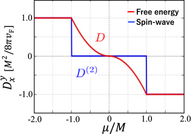
The DMI coefficient in free energy is obtained by integrating with respect to ,
| (43) |
By writing , where is the angle that makes with surface normal, the integration is carried out as
| (44) |
and we obtain
| (47) |
Interestingly, this is finite even when lies in the gap (). This feature is different from , which vanishes there. Thus we have a first example that demonstrates .
Though is typically nonzero even in the gap, it is an odd function of and vanishes at (i.e., in the ground or equilibrium state). A finite DMI in the gap, realized at , may be probed if the chemical potential is tuned by, e.g., gating or impurity doping.
The mathematical reason why is nonzero (while ) in the gap is that at given is contributed from at smaller because of the -integration. That is, even when lies in the gap at some given , if it is nonzero (), it enters the band at smaller , at which is nonzero and contributes to . Physically, it means that twisting the magnetization changes the electronic energy in a chirality-dependent way even in the insulating state.
The factor indicates that a Néel type spin twist is favored.
III.3 Rashba ferromagnet
As a next example, we consider 2D electrons with Rashba SOC,
| (48) |
where with electron (or effective) mass , and is the Rashba constant. In evaluating the DMI coefficients, we assume is perpendicular to the 2D plane. The electron energy is given by
| (49) |
For , there is a Dirac point at , but a finite eliminates it by opening an exchange gap of magnitude . (In this subsection, we assume for simplicity, but the results do not depend on the sign of .) For , the band structure is similar to that of ferromagnets, which is dominated by the exchange splitting [see the inset of Fig. 2 (b)]. For , the shape of the lower band becomes wine-bottle-like [Fig. 2 (c), inset]. We call the former band structure “ferromagnetic type” and the latter “wine-bottle type”. The bottom of the lower band is at energy for ferromagnetic type, and for wine-bottle type.
To study the DMI coefficients, it may be instructive to start with the lowest-order (i.e., first-order) contribution with respect to . In this case, the band structure is of ferromagnetic type, and the DMI coefficient is given by the spin currentKikuchi2016 (see Appendix C). Using Eq. (127) with , , and (density of states), the coefficient of DM free energy is obtained as
| (50) |
where is the magnitude of the magnetization. (The results in this paragraph holds for arbitrary .) This agrees with the result obtained by Ado et al.Ado2018 It is finite only in the half-metallic state, in which the chemical potential crosses only the lower band. The DMI in spin-wave dispersion is obtained as [Eq. (24)]
| (51) |
These results, also plotted in Fig. 2 (a), clearly demonstrate the distinction between and (for ).
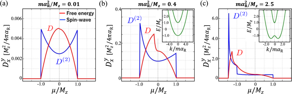
To include higher-order effects with respect to , we use Eq. (36). For a perpendicular magnetizatoin, the -integration can be performed analytically to obtain (for spin waves). The result is
| (52) |
for , whereas it trivially vanishes for . Here, , and are real positive solutions of
| (53) |
with () for the upper (lower) band. Depending on the Fermi-surface morphology, Eq. (52) should be interpreted as follows.
1, For , the contributions from the two Fermi surfaces (each from the upper and lower bands) cancel exactly, resulting in .
2. For , there is no solution for , and the terms that contain in Eq. (52) should be set to zero.
3. For a wine-bottle type band, there is one more region, , where one finds two solutions for . In Eq. (52), the terms that contain should then be understood as the sum of contributions from the two solutions (whereas the terms that contain are set to zero).
The results are plotted in Fig. 2 (b) and (c) by blue lines.
To obtain (for free energy), we first performed the following integration numerically,
| (54) |
which required a careful division into several intervals (see the above result on ). The results are plotted in Fig. 2 (b) and (c) by red lines. We see that it also vanishes for , where both bands have a Fermi surface. This feature was reported in Ref. Ado2018, at the lowest-order in . Here, we have shown it to all orders in .
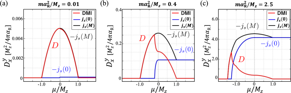
Interestingly, for the present case of perpendicular magnetization, can be expressed by the equilibrium spin-current density, . More precisely, their perpendicular components (perpendicular to ) are mutually related as
| (55) |
This is derived in Appendix D as Eq. (134). This enables us to have analytical expressions of , as displayed in Appendix D.2. Each term in Eq. (55) is plotted in Fig. 3. As seen by the red curves, the agreement between Fig. 2 (calculated by Eq. (54)) and Fig. 3 (calculated by Eq. (55)) is perfect, demonstrating that the spin-current picture works nicely. The following features are seen:
1. At small [Fig. 3 (a)], the spin current at is negligibly small, and the DMI fully reflects the equilibrium spin current at .
2. At larger [Fig. 3 (b), (c)], the spin current develops even at and affects the DMI coefficient. In particular, the abrupt drop in with a cusp is due to the subtraction of the spin current at .
3. When both bands are occupied (), the spin currents are nonvanishing but independent of . Therefore, the DMI coefficient vanishes.
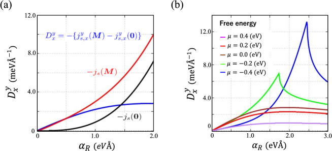
In Ref. Freimuth2017, , it was shown by explicit calculations that deviates from at large when the nonlinear dependence on becomes appreciable. In Fig. 4 (a), we show the same plot but using our spin-current formula, Eq. (55), for . Our plot for (blue line) agrees well with the one presented in Ref. Freimuth2017, (not shown); in a closer look, there is a slight disagreement, which may be attributed to the use of different DMI formula here and in Ref. Freimuth2017, . The DMI coefficient for several choices of are plotted in Fig. 4 (b).
III.4 Magnetic Weyl semimetal
Finally, we consider a magnetic Weyl semimetal. We consider a model with two Weyl cones of opposite chirality,Weyl_review ; Kurebayashi2021
| (56) |
where specifies the chirality of the Weyl cones. The magnetization and the chiral asymmetry parameter determine the relative shift of the two Weyl cones in the momentum and energy directions, respectively. The latter () arises when the system lacks spatial inversion symmetry. The model in the present form was used recently in a microscopic study of various types of (current- and charge-induced) spin torques.Kurebayashi2021
Using the formula (36) with , we perform the -integral by shifting the integration variable to eliminate , such that . This shift is done in a chirality-dependent way,com2 which may be justified if the two Weyl cones (with opposite chiralities) can be treated independently, e.g., if the scattering between the two Weyl cones can be neglected. As a result, the DMI coefficient, calculated from Eq. (36),
| (57) |
is independent of . Therefore, and coincide, ; see Eq. (24). This feature is consistent with (see Appendix B.5). The contributions from opposite-chirality branches tend to cancel each other [see the middle in Eq. (57)], and the nonvanishing DMI is obtained only when , consistent with the symmetry requirement. We also note that it is independent of . The factor indicates that the spin-wave Doppler shift is maximal when the propagation direction is parallel (or antiparallel) to the magnetization. The DM free energy is given by
| (58) |
which favors a Bloch-type spin twist.
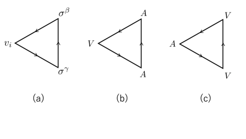
Here, we point out that the DMI in the Weyl system arises as a chiral anomaly. To see this, it is convenient to rephrase the terminology with the language of Weyl fermions: (i) The electron spin is a chiral (or axial-vector) current, . (ii) The magnetization acts as a chiral vector potential, , and acts as a chiral scalar potential, (with metric ). See Ref. HK2021, for a quick overview.
With these terminologies, the DMI is expressed by a triangle diagram with vertices [Fig. 5 (b)], where means the (vector) current vertex , and means the axial(-vector) current vertex . On the other hand, the chiral anomaly is expressed by a triangle diagram with vertices [Fig. 5 (c)]. The former () diagram usually vanishes. However, in the presence of explicit chiral-symmetry breaking (), the process mixes into the process and acquires a finite contribution.
Let us look at the chiral anomaly term explicitly.Zyuzin2012 ; Liu2013 Following Ref. Zyuzin2012, , one can derive an effective action (i.e., time integral of effective Lagrangian) using the Fujikawa method.Fujikawa_book Here, however, we are faced with the case in which varies spatially. To study such a situation, we divide into the average part () and the fluctuation part (), , where is constant and does not depend on space and time. The same is assumed for .
Eliminating the averages ( and ) by a chiral gauge transformation, as done in Ref. Zyuzin2012, , and evaluating the associated change of path integral measure, we obtain the real-time action as
| (59) |
Here, is the chiral electromagnetic field, given explicitly as and . (The familiar chiral anomaly term is obtained if is replaced by real electromagnetic fields, .) The “axion field” is determined by the averaged quantities, . When is static and is uniform, Eq. (59) reduces to
| (60) |
From this, an effective free energy can be obtained by removing the time integral and attaching a minus sign; the result agrees with Eq. (58). Therefore, the DMI in magnetic Weyl semimetals with broken inversion symmetry can be considered to originate from the chiral anomaly.
It may be worth noting that our DMI formula gives the same result, without recourse to such subtle manipulations as represented by the chiral anomaly. This may not be so surprising in view of the fact that the chiral anomaly is well captured within the framework of perturbation theory.Adler1969
| Model | Condition of | |||
|---|---|---|---|---|
| Weyl 111See Eq. (56) for the Hamiltonian, and Eq. (57) for . Here, . | ||||
| MTI surface 222See Eq. (37) for the Hamiltonian, and Eq. (47) for . Here, . | ||||
| Rashba 333See Eq. (48) for the Hamiltonian, Eq. (54) for , and Eq. (52) for with . Here, , and . | ||||
| Weak SOC 444See Eq. (105) for the Hamiltonian, and Eqs (120)-(128) for . We define , and . | , |
IV Discussion
IV.1 vs.
We have emphasized the distinction between and . However, their difference may not be significant if and are weakly dependent on . (If and/or are strictly proportional to , as in the case of magnetic Weyl semimetal, one has .) In the experiment in Ref. Zhou2020, , the authors extracted the scaling ( : saturation magnetization) using the temperature as an implicit parameter. They obtained the exponent , which is consistent with, or not far from, . To see the difference between and experimentally, materials having significantly different from 2 are good candidates.
Explicit relations between and that follow from are summarized in Table 1 for several types of SOC. (See Appendix B.5 for the discussion.) While is expressed by a single quantity for a Weyl semimetal and magnetic topological insulator, two quantities ( and ) are required for Rashba ferromagnet and for systems with general but weak SOC. In all cases studied here, can be expressed solely by (because is related to via ), hence is practically unnecessary. This is reasonable since one can always take the DM free energy as a starting point, where only the term is relevant.
IV.2 Parallel vs. perpendicular components
In comparing and , one needs to pay attention to their vectorial direction relative to , namely, to the components parallel or perpendicular to . (We call the former parallel component and the latter perpendicular component.) While the derived formula for [Eq. (15)] and [Eq. (26)] generally contain both parallel and perpendicular components, only the perpendicular (parallel) component is physically relevant for (), as we have seen in Sec. II.4. Let us denote them and , respectively.
As seen from Table I, and have the same coefficient for the magnetic Weyl semimetal and materials with weak SOC. On the other hand, they have different coefficients for MTI surface electrons and Rashba ferromagnets. In the latter cases, the DMI coefficient determined from the length scale of spin textures and that determined from spin-wave properties can be different.
IV.3 Relation to equilibrium spin current
Kikuchi et al. pointed out that the DMI coefficient is given by the equilibrium spin-current density.Kikuchi2016 Their “spin-current formula” holds at the first order in SOC, thus it is appropriate to systems with weak SOC. Also, they assumed a parabolic electron dispersion as well as SOC that is linear in .
In our formulation, such spin-current formula can be obtained if first-order terms in SOC are retained. This is demonstrated in Appendix C.2, where one can see that the spin-current formula,
| (61) |
holds for arbitrary forms of electron dispersion and SOC. Note that this is restricted to the perpendicular component of . (The parallel component of the spin current vanishes, hence , at the first order in SOC.)
The equality between and the equilibrium spin current can be extended to arbitrary strength of SOC (not just at the lowest order, but to all orders) for a Rashba ferromagnet with perpendicular magnetization. In this case, the above relation is generalized to
| (62) |
in which the spin current at is subtracted. Therefore, the DMI coefficient is equal to the change of the equilibrium spin current induced by the development of , rather than the “preexisting” spin current at . It is known that the equilibrium spin current at is generally nonzero but starts at third order in SOC.Rashba2003 ; Tokatly2008 ; Droghetti2022 Thus, Eq. (62) reduces to Eq. (61) when only the lowest- (i.e., first-) order terms in SOC are considered. Finally, we note that Eq. (62) holds more generally (beyond the Rashba model) if the magnetization is perpendicular to the spin-orbit field. A proof of this is given in Appendix D.
V Summary
In this paper, we have developed a microscopic theory of the DMI mediated by band electrons. In contrast to Moriya’s original theory, which considered Mott insulators, the present one applies to metals, semiconductors, semimetals, and even to band insulators; in fact we have applied it to topological insulator surface states in its insulating state.
We first derived a general formula for the coefficient of the DM free energy in terms of Green’s functions. We then pointed out that the DMI coefficient generally depends on physical quantities, i.e., whether we are looking at (equilibrium) spin structure, torque, or spin waves. This distinction is important in systems with strong SOC, and spectacular examples are given by the Rashba ferromagnet in the half-metallic state (with one partially-occupied band and one empty band) and the MTI surface states in the insulating state. Experimentally, it is expected that the difference between and can be significant when they deviate from the behavior. On the other hand, an exact behavior, hence the equality , has been found in magnetic Weyl semimetal. This is probably an exceptional case among systems with strong SOC, as one might discuss through the analysis of the chiral anomaly.
Also, we have generalized the spin-current formula for the coefficient of the DM free energy, which was known to hold in systems with weak SOC, to the case of strong SOC. Under the assumption that the magnetization is perpendicular to the spin-orbit field, the DMI coefficient is proportional to the equilibrium spin current induced by the coupling to the magnetization.
acknowledgement
We would like to thank J. J. Nakane for his helpful discussion including his suggestion of Eq. (69). H. K. is indebted to T. Ikeda for an early-stage collaboration, and to K.-J. Lee and C.-Y. You for stimulating discussion. Y. H. would like to take this opportunity to thank the “Nagoya University Interdisciplinary Frontier Fellowship” supported by Nagoya University and JST, the establishment of university fellowships towards the creation of science technology innovation, Grant Number JPMJFS2120. This work is also supported by JSPS KAKENHI Grant Numbers JP15H05702, JP17H02929, JP19K03744, and 21H01799.
Appendix A Derivation of general formula
A.1 Basic derivation
In this Appendix, we derive the general expression for the DMI coefficient using the model described in Sec. II.1. We write the exchange coupling as
| (63) |
and treat it as a perturbation but to an infinite order. With the expansion formula, Eq. (9), the free energy is calculated as
| (64) |
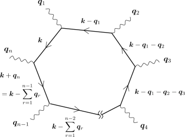
where is given by Eq. (8). Note that there remains a symmetry factor of in the th-order diagram, which is characteristic to free energy.AGD The external wave vectors are supplied from the magnetization, . We are interested in the terms which are first order in either of , and extract them from the Green’s functions to first order. For example, the th Green’s function (counted from left) having momentum is expanded as
| (65) |
up to . It is convenient to first focus on a particular momentum (), collect all terms linear in , and then sum over . In th-order diagrams, the momentum runs from the th to the th , and its contributions are extracted as
| (66) |
where . Here, having extracted , we have set
| (67) |
(note the constraint, ) and wrote for . [The procedure (67) is actually not necessary, and will be relaxed later.] Thus, , where is the uniform magnetization. By summing over and writing as , we obtain
| (68) |
To calculate the -sum, we use the formula,
| (69) |
with . The result is
| (70) |
In the last expression, we introduced
| (71) |
with uniform . To take the -sum, we note that it has the form,
| (72) |
Expanding in powers of , , we find
| (73) |
Therefore, we obtain
| (74) |
Integrating by parts with respect to , we see that the coefficient of is antisymmetric with respect to and . Therefore, can be written in the form,
| (75) |
and the coefficient is given by
| (76) |
If we regard is an integration variable, we can also write
| (77) |
where the integration is done with respect to the magnitude, , while keeping the direction constant.
A.2 On spatial dependence of in
As mentioned near the beginning of Sec. II.3, one can relax the condition of spatial uniformity of on which depends. To show this, one may proceed in the same way as in the preceding subsection using as the unperturbed Green’s function
| (78) |
with spatially nonuniform . In the -representation, this has off-diagonal components. Treating as a matrix in an infinite-dimensional Hilbert space, we can repeat the same manipulation and obtain
| (79) |
where is the velocity operator, and Tr means the trace over all single-particle states (which generalizes the sum over , spin, and band). This corresponds to retaining all the ’s in the preceding subsection, without recourse to the approximation (67).
Appendix B Calculation of free energy variations
In this Appendix, we calculate first- and second-order variations of the DM free energy functional,
| (80) |
under a small change . Note that is in general a function of . In the following calculation, it is convenient to define
| (81) |
and write
| (82) |
B.1 First-order variation
We start with the first-order variation,
| (83) |
where . Integrating the second term by parts, dropping the surface term, and using , we have
| (84) |
where we defined
| (85) |
with .
B.2 Second-order variation
B.3 General formula for
As shown in the preceding subsection, for given (or ), one can calculate and as
| (93) |
or
| (94) |
where and . These relations hold generally among , and , which are defined by Eqs. (80), (84), and (90) [and (92)], respectively. If the explicit expression for , Eq. (77), is used, one can prove (see the next subsection)
| (95) |
and Eq. (94) reduces to
| (96) |
Thus, we find a general formula for ,
| (97) |
which does not involve the - (or -) integration. Conversely, if is given, can be obtained by integration,
| (98) |
where and . The integration is done with respect to the magnitude of , with the direction kept fixed.
B.4 Proof of
To prove , we use Eq. (76) and write
| (99) |
Since only the integrand,
| (100) |
depends on , it is sufficient to prove
| (101) |
Using , one has
| (102) |
which consists of terms of the form,
| (103) |
Noting and integrating by parts, we find
| (104) |
hence, . This means that the right-hand side of Eq. (102) vanishes, proving Eq. (101), thus .
B.5 Other consequences of
The condition also provides some insight into the connection between the functional form (i.e., dependence on ) and the tensorial structure (i.e., dependence on and ) of .
If has the form, , in 3D, where , the above condition says that does not depend on . It then follows from Eq. (24) that . This occurs in magnetic Weyl semimetals, as we have seen in Sec. III B.
If has the form, , where is the antisymmetric tensor in 2D, does not depend on the in-plane components, and . This is the case for topological insulator surface states. Indeed, depends only on , as shown in Ref. Wakatsuki2015, and also in Sec. III C.
Unfortunately, such analysis is not effective for a Rashba ferromagnet, in which takes the form, . While the -term does not contribute to the DM free energy, its presence hinders the extraction of any information on from . Similar feature exists also in the weak SOC case, as studied in Appendix C.1.
These are summarized in Table I.
Appendix C Weak spin-orbit coupling
In this section, we show that at the first order in SOC, the DMI coefficient (in free energy) is given by the equilibrium spin-current density. Such relation was found in Ref. Kikuchi2016, , and here we make a slight generalization. Since the SOC is treated perturbatively, topological materials are not eligible.
We consider the Hamiltonian
| (105) |
where . The second term describes the SOC with strength . A free electron model would assume and , as in Ref. Kikuchi2016, , but here, we leave and to be arbitrary functions of . As shown below, even with this setting, the DMI coefficient is still given by the equilibrium spin current at the first order in .
The full Green’s function is given by
| (106) |
with . We expand it up to the first order in , , where
| (107) |
is at , with .
C.1 DMI coefficient
The DMI coefficient (15) at the first-order in is then
| (108) |
where we used with . The spin trace is taken as
| (109) |
Since the -parallel component of does not contribute to the DM free energy, one may drop the second term () and thereby define . The -integration can be done analytically,
| (110) | ||||
| (111) |
where is the component perpendicular to . In the last equality, we noted
| (112) |
and made an integration by parts.
As to the parallel component of , Eq. (109) leads to
| (113) |
This is consistent with the analysis summarized in Table I.
C.2 Equilibrium spin-current density
Next, we express the equilibrium spin current in terms of Green’s functions. The spin current is expressed as
| (114) |
where . Thus,
| (115) |
In the second line, we retained only the first-order terms in . The spin trace is calculated as
| (116) |
We first note that the parallel component vanishes,
| (117) |
because of Eq. (112). Thus, the spin current consists purely of the perpendicular component,
| (118) |
Comparing this with Eq. (111), we see that
| (119) |
confirming that our general formula reduces to the spin-current formula of Ref. Kikuchi2016, at weak SOC. We emphasize that this holds even when and are arbitrary functions of , which was not obvious from the derivation in Ref. Kikuchi2016, .
C.3 Explicit evaluation
Finally, we evaluate the results explicitly for free electrons in dimensions. We start with general and , and then specialize in stages to and .
Defining and , and using and , Eq. (111) is calculated as follows,
| (120) |
where is the Fermi distribution function and . The last expression shows that is proportional to at small (). This fact was pointed out in Ref. Freimuth2017, in a different formulation. These hold for general and .
For (but with general ), is expressed as
| (121) |
where is the thermodynamic potential of spin- electrons, and is the total electron density. The full and are obtained as
| (122) | |||
| (123) |
with
| (124) | ||||
| (125) | ||||
| (126) |
where is the electron density at (for given ), and is the thermally-averaged density of states. Here we used and as listed in Table 1.
Finally, for and , becomes Ikeda2013
| (127) |
at , where with Fermi energy . For , in which there are two Fermi surfaces, we have
| (128) |
where is the Gamma function. For , where there is only one Fermi surface, we have
| (129) |
Appendix D Generalized spin-current formula
In this Appendix, we show that the spin current formula for the DMI coefficient holds more generally, irrespective of the strength of SOC, if the magnetization vector is perpendicular to the spin-orbit field, . The derivation is based on the same model as in Appendix C, namely, Eq. (105), but the SOC is fully taken into account. The spin current operator is given by Eq. (114), and the equilibrium spin current is expressed as
| (130) |
D.1 Derivation
We first recall that the DMI coefficient is given by Eq. (36), or its -integration,
| (131) |
Assuming is orthogonal to , we focus on the perpendicular component,
| (132) |
where , and we noted . Since is not contained in and , the -integration can be done exactly,
| (133) |
The resulting quantity is identified as the perpendicular component of the equilibrium spin current in Eq. (130). Therefore, we obtain
| (134) |
D.2 Application to Rashba ferromagnet
Let us consider the Rashba ferromagnet studied in Sec. III.3. The equilibrium spin current is expressed as
| (135) |
This can be calculated analytically as follows,
| (136) | ||||
| (137) | ||||
| (138) |
where
| (139) | ||||
| (140) | ||||
| (141) |
At , it becomes
| (142) | ||||
| (143) | ||||
| (144) |
where
| (145) | ||||
| (146) |
These lead to the DMI coefficient, Eq. (134), as follows.
Strong SOC ( or )
| (147) | ||||
| (148) | ||||
| (149) | ||||
| (150) | ||||
| (151) |
Weak SOC ( or )
In this case, 2b), 3b) and 3c) above are replaced by
| (152) | ||||
| (153) | ||||
| (154) |
References
- (1) I. E. Dzyaloshinskii, Sov. Phys. JETP 5, 1259 (1957).
- (2) T. Moriya, Phys. Rev. 120, 91 (1960).
- (3) I. E. Dzyaloshinskii, Sov. Phys. JETP 19, 960 (1964).
- (4) A. Thiaville, S. Rohart, É. Jué, V. Cros, and A. Fert, Europhys. Lett. 100, 57002 (2012).
- (5) G. Chen, T. Ma, A. T. N’Diaye, H. Kwon, C. Won, Y. Wu, and A. K. Schmid, Nat. Commun. 4, 2671 (2013).
- (6) K.-S. Ryu, L. Thomas, S.-H. Yang, and S. Parkin, Nat. Nanotechnol. 8, 527 (2013).
- (7) S. Emori, U. Bauer, S.-M. Ahn, E. Martinez, and G. S. D. Beach, Nat. Mater. 12, 611 (2013).
- (8) J. Torrejon, J. Kim, J. Sinha, S. Mitani, M. Hayashi, M. Yamanouchi, and H. Ohno, Nat. Commun. 5, 4655 (2014).
- (9) A. N. Bogdanov, and D. A. Yablonskii, Sov. Phys. JETP 68, 101 (1989).
- (10) U. K. Rössler, A. N. Bogdanov, and C. Peiderer, Nature(London) 442, 797 (2006).
- (11) S. Mühlbauer, B. Binz, F. Jonietz, C. Pfleiderer, A. Rosch, A. Neubauer, R. Georgii, and P. Böni, Science 323, 915 (2009).
- (12) X. Z. Yu, Y. Onose, N. Kanazawa, J. H. Park, J. H. Han, Y. Matsui, N. Nagaosa, and Y. Tokura, Nature 465, 901 (2010).
- (13) S. Heinze, K. von Bergmann, M. Menzel, J. Brede, A. Kubetzka, R. Wiesendanger, G. Bihlmayer, and S. Blügel, Nat. Phys. 7, 713 (2011).
- (14) N. Nagaosa and Y. Tokura, Nat. Nanotechnol. 8, 899 (2013).
- (15) G. Shirane, R. Cowley, C. Majkrzak, J. B. Sokoloff, B. Pagonis, C. H. Perry, and Y. Ishikawa, Phys. Rev. B 28, 6251 (1983).
- (16) K. Ishimoto, Y. Yamaguchi, S. Mitsuda, M. Ishida, and Y. Endoh, J. Magn. Magn. Mater. 54 1003 (1986).
- (17) Y. Iguchi, S. Uemura, K. Ueno, and Y. Onose, Phys. Rev. B 92, 184419 (2015).
- (18) S. Seki, Y. Okamura, K. Kondou, K. Shibata, M. Kubota, R. Takagi, F. Kagawa, M. Kawasaki, G. Tatara, Y. Otani, and Y. Tokura, Phys. Rev. B 93, 235131 (2016).
- (19) T. J. Sato and D. Okuyama, T. Hong, A. Kikkawa, Y. Taguchi, T. H. Arima, and Y. Tokura, Phys. Rev. B 94, 144420 (2016).
- (20) R. Takagi, D. Morikawa, K. Karube, N. Kanazawa, K. Shibata, G. Tatara, Y. Tokunaga, T. Arima, Y. Taguchi, Y. Tokura, and S. Seki, Phys. Rev. B 95, 220406(R) (2017).
- (21) A. Hrabec, N. A. Porter, A. Wells, M. J. Benitez, G. Burnell, S. McVitie, D. McGrouther, T. A. Moore, and C. H. Marrows, Phys. Rev. B 90 020402(R) (2014).
- (22) R. A. Khan, P. M. Shepley, A. Hrabec, A. W. J. Wells, B. Ocker, C. H. Marrows, and T. A. Moore, Appl. Phys. Lett. 109 132404 (2016).
- (23) C.-F. Pai, M. Mann, A. J. Tan, and G. S. D. Beach, Phys. Rev. B 93, 144409 (2016).
- (24) D. Li, R. Ma, B. Cui, J. Yun, Z. Quan, Y. Zuo, L. Xi, and X. Xu, Appl. Surf. Sci. 513, 145768 (2020).
- (25) Y. Zhou, R. Mansell, S. Valencia, F. Kronast, and S. van Dijken, Phys. Rev. B 101, 054433 (2020).
- (26) J. A. Garlow, S. D. Pollard, M. Beleggia, T. Dutta, H. Yang, and Y. Zhu, Phys. Rev. Lett. 122, 237201 (2019).
- (27) S. Schlotter, P. Agrawal, and G. S. D. Beach, Appl. Phys. Lett. 113, 092402 (2018).
- (28) M. Baćani, M. A. Marioni, J. Schwenk, and H. J. Hug, Sci. Rep. 9, 3114 (2019).
- (29) P. Agrawal, F. Büttner, I. Lemesh, S. Schlotter, and G. S. D. Beach, Phys. Rev. B 100, 104430 (2019).
- (30) K. Zakeri, Y. Zhang, J. Prokop, T.-H. Chuang, N. Sakr, W. X. Tang, and J. Kirschner, Phys. Rev. Lett. 104, 137203 (2010); K. Zakeri, Y. Zhang, T.-H. Chuang, and J. Kirschner, Phys. Rev. Lett. 108, 197205 (2012).
- (31) H. S. Körner, J. Stigloher, H. G. Bauer, H. Hata, T. Taniguchi, T. Moriyama, T. Ono, and C. H. Back, Phys. Rev. B 92, 220413(R) (2015).
- (32) J. M. Lee, C. Jang, B.-C. Min, S.-W. Lee, K.-J. Lee, and J. Chang, Nano Lett. 16, 62 (2015).
- (33) J. Cho, N.-H. Kim, S. Lee, J.-S. Kim, R. Lavrijsen, A. Solignac, Y. Yin, D.-S. Han, N. J. J. van Hoof, H. J. M. Swagten, B. Koopmans, and C.-Y. You, Nat. Commun. 6, 7635 (2015).
- (34) M. Belmeguenai, J.-P. Adam, Y. Roussigné, S. Eimer, T. Devolder, J.-V. Kim, S. M. Cherif, A. Stashkevich, and A. Thiaville, Phys. Rev. B 91, 180405(R) (2015).
- (35) K. Di, V. L. Zhang, H. S. Lim, S. C. Ng, M. H. Kuok, J. Yu, J. Yoon, X. Qiu, and H. Yang, Phys. Rev. Lett. 114, 047201 (2015).
- (36) H. T. Nembach, J. M. Shaw, M. Weiler, E. Jué, and T. J. Silva, Nat. Phys. 11, 825 (2015).
- (37) A. A. Stashkevich, M. Belmeguenai, Y. Roussigné, S. M. Cherif, M. Kostylev, M. Gabor, D. Lacour, C. Tiusan, M. Hehn, Phys. Rev. B 91, 214409 (2015).
- (38) A. K. Chaurasiya, C. Banerjee, S. Pan, S. Sahoo, S. Choudhury, J. Sinha, and A. Barman, Sci. Rep. 6, 32592 (2016).
- (39) X. Ma, G. Yu, X. Li, T. Wang, D. Wu, K. S. Olsson, Z. Chu, K. An, J. Q. Xiao, K. L. Wang, and X. Li, Phys. Rev. B 94, 180408(R) (2016).
- (40) A. Hrabec, M. Belmeguenai, A. Stashkevich, S. M. Chérif, S. Rohart, Y. Roussigné, and A. Thiaville, Appl. Phys. Lett. 110, 242402 (2017).
- (41) R. M. Rowan-Robinson, A. A. Stashkevich, Y. Roussigné, M. Belmeguenai, S.-M. Chérif, A. Thiaville, T. P. A. Hase, A. T. Hindmarch, and D. Atkinson, Sci. Rep. 7, 16835 (2017).
- (42) X. Ma, G. Yu, S. A. Razavi, S. S. Sasaki, X. Li, K. Hao, S. H. Tolbert, K. L. Wang, and X. Li, Phys. Rev. Lett. 119, 027202 (2017).
- (43) N.-H. Kim, Qurat-ul-ain, J. Kim, E. Baek, J.-S. Kim, H.-J. Park, H. Kohno, K.-J. Lee, S. H. Rhim, H.-W. Lee, and C.-Y. You, Phys. Rev. B 105, 064403 (2022).
- (44) M. Kuepferling, A. Casiraghi, G. Soares, G. Durin, F. Garcia-Sanchez, L. Chen, C. H. Back, C. H. Marrows, S. Tacchi, and G. Carlotti, Rev. Mod. Phys. 95, 015003 (2023).
- (45) M. Heide, G. Bihlmayer, S. Blügel, Phys. Rev. B 78, 140403(R) (2008).
- (46) M. I. Katsnelson, Y. O. Kvashnin, V. V. Mazurenko, and A. I. Lichtenstein, Phys. Rev. B 82, 100403(R) (2010).
- (47) J. Gayles, F. Freimuth, T. Schena, G. Lani, P. Mavropoulos, R. A. Duine, S. Blügel, J. Sinova, and Y. Mokrousov, Phys. Rev. Lett. 115, 036602 (2015).
- (48) T. Koretsune, N. Nagaosa, and R. Arita, Sci. Rep. 5, 13302 (2015).
- (49) R. Wakatsuki, M. Ezawa, and N. Nagaosa, Sci. Rep. 5, 13638 (2015).
- (50) T. Kikuchi, T. Koretsune, R. Arita, and G. Tatara, Phys. Rev. Lett. 116, 247201 (2016).
- (51) F. Freimuth, S. Blügel, and Y. Mokrousov, Phys. Rev. B 96, 054403 (2017).
- (52) T.Koretsune, T. Kikuchi, and R. Arita, J. Phys. Soc. Japan 87, 041011 (2018).
- (53) I. A. Ado, A. Qaiumzadeh, R. A. Duine, A. Brataas, and M. Titov, Phys. Rev. Lett. 121, 086802 (2018).
- (54) M. Kataoka, O. Nakanishi, A. Yanase, and J. Kanamori, J. Phys. Soc. Japan 53, 3624 (1984).
- (55) A. A. Abrikosov, L. P. Gor’kov, I. E. Dzyaloshinskii, Methods of Quantum Field Theory in Statistical Physics (Pergamon Press, Oxford).
- (56) G. Tatara, H. Kohno, and J. Shibata, Phys. Rep. 468, 213 (2008).
- (57) R. L. Melcher, Phys. Rev. Lett. 30, 125 (1973).
- (58) M. Kataoka, J. Phys. Soc. Japan 56, 3635 (1987).
- (59) L. Udvardi and L. Szunyogh, Phys. Rev. Lett. 102, 207204 (2009).
- (60) M. Z. Hasan and C. L. Kane, Rev. Mod. Phys. 82, 3045 (2010); X.-L. Qi and S.-C. Zhang, Rev. Mod. Phys. 83, 1057 (2011).
- (61) Y. Tokura, K. Yasuda, and A. Tsukazaki, Nat. Rev. Phys. 1, 126 (2019).
- (62) This information is not lost in our formulation. In fact, anisotropic exchange interaction can be included in , and thus .
- (63) P. Hosur and X. Qi, C. R. Phys. 14, 857 (2013); N. P. Armitage, E. J. Mele, and A. Vishwanath, Rev. Mod. Phys. 90, 015001 (2018); B. Q. Lv, T. Qian, and H. Ding, Rev. Mod. Phys. 93, 025002 (2021).
- (64) D. Kurebayashi, Y. Araki, and K. Nomura, J. Phys. Soc. Japan 90, 084702 (2021).
- (65) We believe this is allowed in the calculation of the coefficient , in contrast to the calculation of the whole term (chiral anomaly) presented in Eq. (60).
- (66) H. Kohno, JPSJ News Comments 18, 13 (2021).
- (67) A. A. Zyuzin and A. A. Burkov, Phys. Rev. B 86, 115133 (2012).
- (68) C.-X. Liu, P. Ye, and X.-L. Qi, Phys. Rev. B 87, 235306 (2013).
- (69) K. Fujikawa and H. Suzuki, Path Integrals and Quantum Anomalies (Clarendon Press, Oxford, 2004).
- (70) S. L. Adler, Phys. Rev. 177, 2426 (1969); J. S. Bell and R. Jackiw, Nuovo Cimento A 60, 47 (1969).
- (71) E. I. Rashba, Phys. Rev. B 68, 241315(R) (2003).
- (72) I. V. Tokatly, Phys. Rev. Lett. 101, 106601 (2008).
- (73) A. Droghetti, I. Rungger, A. Rubio, and I. V. Tokatly, Phys. Rev. B 105, 024409 (2022).
- (74) T. Ikeda, Master thesis (Osaka University, March 2013).