Visualizing data augmentation in deep speaker recognition

Abstract

Visualization is of great value in understanding the internal mechanisms of neural networks. Previous work found that LayerCAM is a reliable visualization tool for deep speaker models. In this paper, we use LayerCAM to analyze the widely-adopted data augmentation (DA) approach, to understand how it leads to model robustness. We conduct experiments on the VoxCeleb1 dataset for speaker identification, which shows that both vanilla and activation-based (Act) DA approaches enhance robustness against interference, with Act DA being consistently superior. Visualization with LayerCAM suggests DA helps models learn to delete temporal-frequency (TF) bins that are corrupted by interference. The ‘learn to delete’ behavior explained why DA models are more robust than clean models, and why the Act DA is superior over the vanilla DA when the interference is nontarget speech. However, LayerCAM still cannot clearly explain the superiority of Act DA in other situations, suggesting further research.

Index Terms: speaker recognition, visualization, data augmentation

1 Introduction

Despite the great advance recently obtained in the field of speaker recognition [1, 2, 3, 4, 5], ambient noise and other interference severely degrade the performance of speaker recognition systems [6, 7]. To improve robustness, modern deep speaker models, e.g., the x-vector [4], extensively rely on data augmentation (DA). Popular DA methods include gain augmentation, noise mixing, reverberation simulation, time stretch, and SpecAug [8, 9]. These DA methods have been widely used by nearly all speaker recognition systems [10, 11, 12, 13] and implemented in most known toolkits, e.g, Kaldi [14] and Speechbrain [15].

The core idea of DA is to increase the size and diversity of the training set by generating new samples from the existing training data. With the newly generated data, the model is supposed to learn speaker patterns in more complex conditions, hence leading to increased robustness. Although the main principle of DA is widely adopted, we still have not a clear understanding of how DA models behave differently from clean models, and in which way the DA models gain robustness against interference. A lack of such understanding prevents us from interpreting the output of DA models (e.g., confidence estimation), designing smart verification/identification protocols (e.g., repetition policy), and constructing more efficient DA processes. Unfortunately, deciphering deep speaker models turns out to be highly difficult, as neural networks are notorious for their black-box nature.

Recently, various visualization methods have been developed to understand the internal mechanisms of deep models, and remarkable success has been achieved particularly in the computer vision field [16, 17, 18]. For speaker recognition, there are also some attempts to use such visualization tools to explain deep speaker models. For example, Zhou et al. [19] used Grad-CAM [20] to compare ResNet and Res2Net. They found that the saliency map produced by Grad-CAM is more stable with Res2Net compared with ResNet, thus explaining the advantage of Res2Net. In another work, Himawan et al. [21] used Grad-CAM to analyze the difference between genuine and spoof speech from the perspective of deep CNN anti-spoof models. They found that the CNN model identifies spoof speech by looking into high-frequency components. A potential problem of these studies is that the visualization tools are used `off-the-shelf', without inquiring if the explanation generated by these tools is correct. Recent research [22] showed a surprising discovery: blindly using the visualization tools may produce a misleading explanation for deep speaker models. The authors studied various algorithms in the CAM family, and found that only LayerCAM [23] can identify the important temporal-frequency (TF) bins and offer a reliable explanation.

In this paper, we use LayerCAM as the probing tool to understand the contribution of data augmentation in training deep speaker models. To simplify the study, we focus on a particular and mostly used DA approach — interference mixing, and test only known interference. We use LayerCAM to study two DA algorithms: vanilla DA and activation-based DA (Act DA). The latter involves an additional loss that enforces augmented speech close to the original clean speech in the embedding space.

A speaker identification (SID) experiment was designed to test and analyze the DA methods, using the VoxCeleb1 dataset. The results show that DA contributes by letting the models `learn to delete', i.e., learn to detect temporal-frequency (TF) bins belonging to or corrupted by interference. This `learn to delete' hypothesis provides a possible explanation for the DA approach and sheds more light on how deep speaker models gain their decisions from speech signals.

2 Revisit LayerCAM

LayerCAM [22, 23] is a vital tool for visualizing CNN models. It constructs a saliency map of the same size as the original input (e.g., a picture or a Mel spectrogram). This saliency map shows the important regions when a CNN model tries to identify a particular class.

Let $f$ denote the speaker classifier instantiated by a CNN, and $\theta$ represents its parameters. For a given input $x$ from class $c$, the prediction score (posterior probability) for the target class can be computed by a forward pass:

$$y^{c}=f_{c}(x;\theta).$$ (1)

Secondly, the weight for $k$-th activation map $A^{k}$ for class $c$ at location ($i,j$) is defined as the gradient at that location:

$$w_{ij}^{kc}=\text{ReLU }(\frac{\partial y^{c}}{\partial A_{ij}^{k}}).$$ (2)

Finally, the saliency map is produced as follows:

$$S_{ij}^{c}=\text{ReLU }(\sum_{k}w_{ij}^{kc}\cdot{A_{ij}^{k}}).$$ (3)

We normalize $S_{ij}^{c}$ to the range [0,1] following the same procedure recommended in [22]. Moreover, $S_{ij}^{c}$ is computed for each CNN layer, and we fuse $S_{ij}^{c}$ of four layers (ResNetBlock1-ResNetBlock4) by element-wise average manner, as suggested in [22].

3 Data augmentation

In this paper, we use LayerCAM as a visualization tool to analyze two DA variants: the vanilla DA and the Act DA which involves an additional loss in the embedding space.

3.1 Vanilla DA

For the Vanilla DA, we randomly sample interference signals from MUSAN [24] dataset and mix it with the target speech. Let $x$ denote clean speech, $\tilde{x}$ is an augmented version derived from $x$ by:

$$\tilde{x}=x+\alpha n\ \ \ \ \ \ \alpha\sim\text{Uniform}(0.1,2.0)$$ (4)

where $n$ is an interference signal sampled from the MUSAN dataset. The loss function is written by:

$$L_{\text{Vanilla-DA}}=L(x)+L(\tilde{x})$$ (5)

where $L$ is the objective function used for training the deep speaker model, which is the cross-entropy loss in our study. There are three types of interference in MUSAN: noise, speech, and music. As mentioned, we train and test DA models for the three interference separately, with the sake of simplifying the analysis.

3.2 Act DA

We design a variant of the vanilla DA named Act DA. It introduces an extra constraint that enforces the clean and augmented speech close to each other in the embedding space. Let $e(x)$ denote the embedding of $x$, the loss function of the Act DA is as follows:

$$L_{\text{Act-DA}}=L(x)+L(\tilde{x})+||e(x)-e(\tilde{x})||^{2}$$ (6)

4 Experiment

In this section, we first validate the robustness of the two DA methods with a speaker identification task, and secondly apply LayerCAM to explain how DA improves the robustness of deep speaker models.

4.1 Power of data augmentation

In this section, we design a speaker identification (SID) task to demonstrate the power of data augmentation. The structure of the model is ResNet34L with squeeze-and-excitation (SE) layers [25]. The dataset used to conduct the experiments is Voxceleb1 [26], and we use the standard development set to train the model and the evaluation set for SID to test the performance. There are 1,251 speakers in total. The training is conducted following the voxceleb/v2 recipe of the Sunine toolkit. Note that the speakers in the test set also appear in the training set, so the outputs of the ResNet34L network are used directly to identify the target speaker.

The MUSAN database is used to sample interference signals, including three types: noise, speech, and music. As mentioned, we train DA models with each type of interference, and test the models on speech with the same interference. This allows us to focus on how a DA model learns to deal with interference it sees during training. More complicated cross-condition generalization will be left for future work.

Table 1 shows the Top-1/5/10 accuracy of the models trained/tested with each type of interference. It can be seen that the clean model can obtain pretty good performance on clean speech, however, it suffers significant performance degradation on noisy speech no matter which type of interference. The DA models demonstrate remarkable performance improvement on noisy speech without much impact on clean speech. Interestingly, the Act DA model shows a more significant improvement than the vanilla DA model, and the advantage is more evident in the scenario with speech interference.

Table 1: Accuracy(%) of models tested under different interference conditions, with/without data augmentation. Note that for noise/speech/music conditions, DA models are trained with matched interference; for the clean condition, the results with DA models are the mean of the three DA models trained with different interference.

Conditions		Base	Vanilla DA	Act DA
Clean	Top-1	96.64	95.68	95.35
	Top-5	98.80	98.63	98.49
	Top-10	99.21	99.09	98.97
Noise	Top-1	47.30	73.40	75.02
	Top-5	57.30	82.25	83.74
	Top-10	61.23	85.09	86.75
Speech	Top-1	42.31	75.53	81.08
	Top-5	53.96	86.23	91.10
	Top-10	58.24	89.44	93.63
Music	Top-1	26.47	49.74	53.23
	Top-5	35.05	61.37	64.68
	Top-10	38.71	65.47	68.25

The above results confirm that DA training can lead to a significant improvement in model robustness, and the Act DA training leads to further gains. However, how the improvement is obtained by DA and how Act DA wins vanilla DA is still vague. We will apply LayerCAM to get a deeper understanding.

4.2 Concatenated interference

We start from a simple scenario where the target speech and the interference are concatenated. The saliency maps found by LayerCAM are shown in Figure 1, where each column is a speech that is sampled from the test set and concatenated by a particular interference. It can be seen that both the clean model and the two DA models can identify the interference segment, while the DA models (3rd and 4th rows) work much better than the clean model (2nd row).

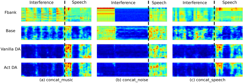
Figure 1: Saliency maps of three utterances sampled the test set and concatenated with different types of interference. The first row shows the Fbank features, and the rest rows show the saliency maps produced by LayerCAM with the clean model (2nd row), the vanilla DA model (3rd row) and the Act DA model (4th row). The saliency values have been scaled to the range [0,1], and high values represent important regions and are shown by warm color.

To quantify the performance of different models in identifying interference regions, we compute the speech preservation ratio (SPR) and interference preservation ratio (IPR) with the VoxCeleb1 test set. Specifically, we sum the saliency values across the frequency axis to get the saliency value for each frame, and if the value is above 15 (empirical set) the frame is regarded to belong to the target speech, otherwise, it belongs to the interference. SPR and IPR are defined as the retention ratio of the target speech and the interference signal after the above dichotomy, respectively.

Table 2: Quality of saliency maps produced by LayerCAM with different models. SPR: speech preservation ratio; IPR: interference preservation ratio.

Conditions		Base	Vanilla DA	Act DA
SPR($\uparrow$)	Noise	95.8%	93.4%	94.2%
	Speech	92.8%	94.9%	94.2%
	Music	95.6%	92.5%	93.0%
IPR($\downarrow$)	Noise	42.3%	5.5%	9.5%
	Speech	81.9%	47.7%	25.7%
	Music	43.7%	5.2%	8.3%

The results are shown in Table 2. First of all, the SPR values of all the models are not significantly different, suggesting that the speech segments are all well identified by all the models. However, the IPR values show much difference: the DA models identify the interference much more successfully than the clean model, indicating that by DA training, the models have learned what is useless. We, therefore, conjecture that the main role that DA plays is to learn how to delete interference, instead of identifying speech segments. This trend is most clear in the test with the speech interference, where the DA models are much stronger than the clean model in identifying and removing the interference, and the Act DA model is substantially stronger than the vanilla DA model. Considering the superior performance of Act DA in the SID experiment, we hypothesize that the `learn to delete’ feature contributes the most to the success of DA training.

4.3 Overlapped interference

In this section, we consider a more complicated scenario where the target speech and the interference are overlapped. We start by visualizing the saliency maps and then conduct quantitative analysis.

4.3.1 Saliency map

The saliency maps of three samples overlapped with different types of interference are shown in Figure 2. To make the presentation clear, the Fbank features of the target speech and the interference are shown separately in the first and the second row.

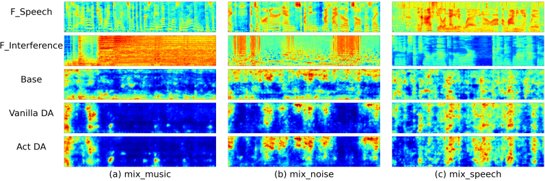
Figure 2: Saliency maps of speech overlapped with three types of interference (music, noise, speech). The first and second rows are Fbank features of the target speech and interference, and the rest rows are the saliency maps produced by LayerCAM for the clean model (3rd row), vanilla DA model (4th row), and Act DA model (5th row).

We draw some similar conclusions as in the scenario with concatenated interference. For example, the DA models are more powerful in identifying the interference region than the clean model, and the Act DA model works better than the vanilla DA model under the condition with speech interference, as it identifies more TF bins with strong interference. This is consistent with the low IPR value that the Act DA model obtains in Table 2. Perhaps the most important observation is that with the two DA models, high saliency values are assigned to the TF regions where the interference is weak, rather than the regions where the target speech is strong. This double confirms the `learn to delete' hypothesis we proposed in Section 4.2.

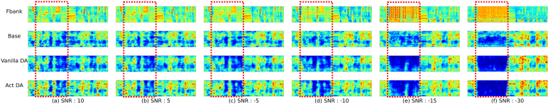
Figure 3: Fbank features (1st row) and saliency maps from the clean model (2nd row) and the two DA models (3rd and 4th rows), when a phone ring is mixed with the target speech in the areas shown by the red boxes. The intensity of the noise is increased gradually from left to right.

4.3.2 Quantity analysis

Since the target speech and interference are overlapped, the SPR/IPR metrics are not suitable anymore for the quantitative analysis. To solve the problem, we borrow some metrics from speech enhancement research. Specifically, the saliency values are treated as soft masks to `denoise' the interfered speech. This can be simply conducted by multiplying the saliency values to the Fbank features of the noisy data and then converting the denoised features to waveforms. The conversion is based on inverse FFT, with the phase spectrogram of the clean speech. For a fair comparison, the noisy speech also undergoes the same re-synthesizing process. We then measure the quality of the denoised speech by PESQ, STOI, and SNR, three popular metrics in speech enhancement, which we assume reflect the quality of the saliency maps.

Table 3: Quality of the denoised speech when applying the saliency values as the denoising masks.

Conditions		Noisy	Saliency Mask
			Base	Vanilla DA	Act DA
Noise	PESQ ($\uparrow$)	1.430	1.442	1.473	1.472
	STOI ($\uparrow$)	0.688	0.689	0.707	0.707
	SNR ($\uparrow$)	-5.358	-4.850	-4.602	-4.548
Speech	PESQ ($\uparrow$)	1.377	1.372	1.387	1.392
	STOI ($\uparrow$)	0.616	0.607	0.628	0.640
	SNR ($\uparrow$)	-5.648	-5.313	-5.129	-4.810
Music	PESQ ($\uparrow$)	1.247	1.249	1.254	1.252
	STOI ($\uparrow$)	0.529	0.529	0.557	0.556
	SNR ($\uparrow$)	-8.277	-7.673	-7.027	-7.141

The results are presented in Table 3. It can be seen that denoising with saliency maps from the clean model (2nd column) indeed leads to marginal but consistent improvement in speech quality, especially in terms of SNR. This indicates that the clean model can detect the interference TF bins to some extent. In comparison, denoising with the saliency maps from the augmented models leads to more significant improvement, indicating that DA models are more powerful in detecting and removing interference. By comparing the two DA models, the Act DA model shows an advantage when the interference is speech, which is consistent with the results in Table 2 and Figure 2.

4.4 Corrupted speech

In the last experiment, we show how clean and DA models treat the speech segments corrupted by interference: will they be still used anyway or simply thrown away? Figure 3 presents a show-case study, where we mix a noise speech (a phone ring) with a target speech and increase the intensity of the noise gradually. The Fbank features of the noisy speech and the saliency maps from different models are shown. Note that the red boxes indicate the speech segment corrupted by the phone ring.

It can be seen that when the noise is weak (SNR = 10, 5), most of the TF bins of the corrupted speech remain, even though some information has been lost due to corruption. When the noise becomes stronger (SNR = -5, -10, -15), the noise has a more impact, especially on the high-frequency region where the energy of human speech is weak [27]. In this scenario, the saliency values of the high-frequency TF bins are reduced, though the low-frequency bins are still retained. When the noise is very strong (SNR = -30), the saliency values of the whole noisy segment are reduced to zero. The above trend is similar with both the clean model and the two DA models, though it is much more clear with the DA models. This suggests that DA models not only learn to delete interference but also learn to delete speech regions if they are severely corrupted.

A deletion test [22, 28] is conducted to verify this behavior quantitatively. In this test, we firstly compute the saliency maps of noisy data, and progressively mask the TF bins of the clean speech whose saliency values in TF bins of the noisy speech are small. Finally, we test the SID accuracy with the masked clean speech using the clean model. If a model tends to delete corrupted speech segments, the performance tested on the masked clean speech with the clean model will drop significantly, as the deleted segments are informative for the clean model.

The results are shown in Figure 4, where each plot shows the SID accuracy when the threshold on the saliency values for the TF bin masking is increased. It can be seen that the DA models exhibit a more significant performance drop, indicating that they delete some speech TF bins that would be useful for the clean model. An interesting observation is that the Act DA model tends to be more aggressive in masking corrupted speech in the condition with speech interference (right plot). This is also consistent with the observation in Figure 3 and explained why Act DA performs significantly better than vanilla DA in that condition as shown in Table 1.

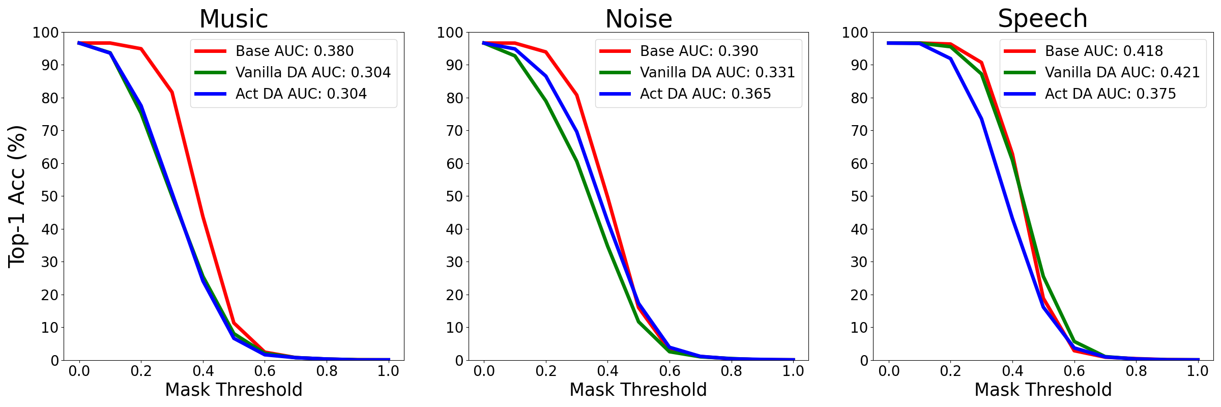
Figure 4: Deletion test to verify that DA models tend to delete more corrupted speech compared to clean models. Clean speech is masked according to the saliency map of noisy speech and then tested with the clean model. Gradually increasing the threshold on the saliency values to be masked gives the curves shown in the three plots. AUC: Area Under the Curve.

5 Conclusions

This paper aims to understand the role that data augmentation plays in speaker recognition, by using LayerCAM as a visualization tool. By speaker identification experiments conducted with the VoxCeleb1 dataset, we found that data augmentation functions by detecting interference regions as well as speech regions corrupted by strong interference, and removing their impact by assigning low saliency values in these regions. We call this the `learn to delete' hypothesis. This hypothesis explains how data augmentation improves model robustness, and explains why an activation-based DA performs better than the vanilla DA when the interference signal is speech.

We admit that the `explanation' is still superficial and far from a full understanding of the working mechanism of deep speaker models. For instance, how the model discovers speaker-related patterns and how DA impacts such discovery thus leading to robustness. Future work will focus on a more zoom-in understanding of the model and more complex robustness that various DA methods and other advanced techniques have contributed.

References

- [1] N. Dehak, P. J. Kenny, R. Dehak, P. Dumouchel, and P. Ouellet, ``Front-end factor analysis for speaker verification,'' IEEE Transactions on Audio, Speech, and Language Processing, vol. 19, no. 4, pp. 788–798, 2010.
- [2] E. Variani, X. Lei, E. McDermott, I. L. Moreno, and J. Gonzalez-Dominguez, ``Deep neural networks for small footprint text-dependent speaker verification,'' in IEEE International Conference on Acoustics, Speech and Signal Processing (ICASSP). IEEE, 2014, pp. 4052–4056.
- [3] L. Li, Y. Chen, Y. Shi, Z. Tang, and D. Wang, ``Deep speaker feature learning for text-independent speaker verification,'' in INTERSPEECH, 2017, pp. 1542–1546.
- [4] D. Snyder, D. Garcia-Romero, G. Sell, D. Povey, and S. Khudanpur, ``X-vectors: Robust DNN embeddings for speaker recognition,'' in IEEE International Conference on Acoustics, Speech and Signal Processing (ICASSP). IEEE, 2018, pp. 5329–5333.
- [5] W. Cai, J. Chen, and M. Li, ``Exploring the encoding layer and loss function in end-to-end speaker and language recognition system,'' arXiv preprint arXiv:1804.05160, 2018.
- [6] K. S. Rao and S. Sarkar, Robust speaker recognition in noisy environments. Springer, 2014.
- [7] T. F. Zheng and L. Li, Robustness-related issues in speaker recognition. Springer, 2017, vol. 2.
- [8] D. S. Park, W. Chan, Y. Zhang, C.-C. Chiu, B. Zoph, E. D. Cubuk, and Q. V. Le, ``Specaugment: A simple data augmentation method for automatic speech recognition,'' in INTERSPEECH, 2019, pp. 2613–2617.
- [9] S. Wang, J. Rohdin, O. Plchot, L. Burget, K. Yu, and J. Černockỳ, ``Investigation of specaugment for deep speaker embedding learning,'' in IEEE International Conference on Acoustics, Speech and Signal Processing (ICASSP). IEEE, 2020, pp. 7139–7143.
- [10] O. Novotnỳ, O. Plchot, P. Matejka, L. Mosner, and O. Glembek, ``On the use of x-vectors for robust speaker recognition.'' in Odyssey, 2018, pp. 168–175.
- [11] M. Zhao, Y. Ma, M. Liu, and M. Xu, ``The speakin system for voxceleb speaker recognition challange 2021,'' arXiv preprint arXiv:2109.01989, 2021.
- [12] L. Li, ``Technical overview for CNSRC 2022,'' Tsinghua University, 2022. [Online]. Available: http://cnceleb.org/workshop
- [13] W. Lin and M.-W. Mak, ``Robust speaker verification using population-based data augmentation,'' in IEEE International Conference on Acoustics, Speech and Signal Processing (ICASSP). IEEE, 2022, pp. 7642–7646.
- [14] D. Povey, A. Ghoshal, G. Boulianne, L. Burget, O. Glembek, N. Goel, M. Hannemann, P. Motlicek, Y. Qian, P. Schwarz et al., ``The Kaldi speech recognition toolkit,'' in IEEE 2011 workshop on automatic speech recognition and understanding, no. CONF. IEEE Signal Processing Society, 2011.
- [15] M. Ravanelli, T. Parcollet, P. Plantinga, A. Rouhe, S. Cornell, L. Lugosch, C. Subakan, N. Dawalatabad, A. Heba, J. Zhong et al., ``SpeechBrain: A general-purpose speech toolkit,'' arXiv preprint arXiv:2106.04624, 2021.
- [16] K. Simonyan and A. Zisserman, ``Very deep convolutional networks for large-scale image recognition,'' arXiv preprint arXiv:1409.1556, 2014.
- [17] M. T. Ribeiro, S. Singh, and C. Guestrin, ````Why should I trust you?'' explaining the predictions of any classifier,'' in Proceedings of the 22nd ACM SIGKDD international conference on knowledge discovery and data mining, 2016, pp. 1135–1144.
- [18] B. Zhou, A. Khosla, A. Lapedriza, A. Oliva, and A. Torralba, ``Learning deep features for discriminative localization,'' in IEEE conference on computer vision and pattern recognition, 2016, pp. 2921–2929.
- [19] T. Zhou, Y. Zhao, and J. Wu, ``Resnext and res2net structures for speaker verification,'' in IEEE Spoken Language Technology Workshop (SLT). IEEE, 2021, pp. 301–307.
- [20] R. R. Selvaraju, M. Cogswell, A. Das, R. Vedantam, D. Parikh, and D. Batra, ``Grad-CAM: Visual explanations from deep networks via gradient-based localization,'' in Proceedings of the IEEE international conference on computer vision, 2017, pp. 618–626.
- [21] I. Himawan, S. Madikeri, P. Motlicek, M. Cernak, S. Sridharan, and C. Fookes, ``Voice presentation attack detection using convolutional neural networks,'' Handbook of Biometric Anti-Spoofing: Presentation Attack Detection, pp. 391–415, 2019.
- [22] P. Li, L. Li, A. Hamdulla, and D. Wang, ``Reliable visualization for deep speaker recognition,'' in INTERSPEECH, 2022, pp. 331–335.
- [23] P.-T. Jiang, C.-B. Zhang, Q. Hou, M.-M. Cheng, and Y. Wei, ``LayerCAM: Exploring hierarchical class activation maps for localization,'' IEEE Transactions on Image Processing, vol. 30, pp. 5875–5888, 2021.
- [24] D. Snyder, G. Chen, and D. Povey, ``Musan: A music, speech, and noise corpus,'' arXiv preprint arXiv:1510.08484, 2015.
- [25] J. Hu, L. Shen, and G. Sun, ``Squeeze-and-excitation networks,'' in Proceedings of the IEEE conference on computer vision and pattern recognition, 2018, pp. 7132–7141.
- [26] A. Nagrani, J. S. Chung, and A. Zisserman, ``VoxCeleb: A large-scale speaker identification dataset,'' in INTERSPEECH, 2017, pp. 2616–2620.
- [27] B. B. Monson, B. Story, and A. Lotto, ``Analysis of high-frequency energy in singing and speech,'' The Journal of the Acoustical Society of America, vol. 131, no. 4, pp. 3378–3378, 2012.
- [28] V. Petsiuk, A. Das, and K. Saenko, ``Rise: Randomized input sampling for explanation of black-box models,'' arXiv preprint arXiv:1806.07421, 2018.