A First-Order Mean-Field Game on a Bounded Domain with Mixed Boundary Conditions

Abstract

This paper presents a novel first-order mean-field game model that includes a prescribed incoming flow of agents in part of the boundary (Neumann boundary condition) and exit costs in the remaining portion (Dirichlet boundary condition). Our model is described by a system of a Hamilton-Jacobi equation and a stationary transport (Fokker-Planck) equation equipped with mixed and contact-set boundary conditions. We provide a rigorous variational formulation for the system, allowing us to prove the existence of solutions using variational techniques. Moreover, we establish the uniqueness of the gradient of the value function, which is a key result for the analysis of the model. In addition to the theoretical results, we present several examples that illustrate the presence of regions with vanishing density.

1 Introduction

This paper studies first-order stationary Mean Field Games (MFG) in a bounded domain under mixed boundary conditions. The precise problem we consider is as follows.

Problem 1 (The Mean-Field Game (MFG)).

Let $\Omega\subset\mathbb{R}^{d}$ be a bounded, open, and connected $C^{1}$–domain whose boundary, $\Gamma=\partial\Omega$, is partitioned into two sets $\Gamma=\overline{\Gamma}_{D}\cup\overline{\Gamma}_{N}$. Let $g$ be a non-decreasing $C^{1}$ function, $j$ be a non-negative function on $\Gamma_{N}$, $H$ be a convex function, and $\psi$ be a continuous function up to the boundary. Solve the following system for $(m,u)$.

$$\begin{cases}H(x,Du)=g(m)&\text{ in }\Omega,\\ -\operatorname*{div}(mD_{p}H(x,Du))=0&\text{ in }\Omega,\end{cases}$$ (1.1)

with the boundary conditions

$$\begin{cases}mD_{p}H(x,Du)\cdot\nu=j(x)&\text{ on }\Gamma_{N},\\ mD_{p}H(x,Du)\cdot\nu\leq 0\,\text{ and }\,u(x)\leq\psi(x)&\text{ on }\Gamma_{D},\\ (\psi-u)mD_{p}H(x,Du)\cdot\nu=0&\text{ on }\Gamma_{D}.\end{cases}$$ (1.2)

Here, $\Gamma_{D}$ and $\Gamma_{N}$ are $(d-1)$–dimensional smooth manifolds, disjoint and open relative to $\Gamma$. The intersection $\overline{\Gamma}_{D}\cap\overline{\Gamma}_{N}$ has (Lebesgue) measure zero, i.e. $\left|\overline{\Gamma}_{D}\cap\overline{\Gamma}_{N}\right|=0$. In the set $\Gamma_{N}$, corresponding to Neumann boundary conditions, we prescribe the flow of incoming agents. In the other set, $\Gamma_{D}$, we prescribe Dirichlet boundary conditions and complementary conditions, which require that $\Gamma_{D}$ set is an exit, not an entrance, and impose an exit cost at points with a positive outflow. Additionally, we denote the contact set between $u$ and $\psi$ (see (1.2)) by $\Gamma_{D}^{1}:=\left\{x\in\Gamma_{D}\ |\ u(x)=\psi(x)\right\}$, while the non-contact set is denoted by $\Gamma_{D}^{0}=\Gamma_{D}\setminus\Gamma_{D}^{1}$. Additional assumptions on the functions $\psi$, $j$, $H$, and $G$ are specified in Section 3. Our stationary Neumann-Dirichlet model (1.1)-(1.2) describes the equilibrium state of a game in a bounded domain, whose boundary is split into two parts: one from which the agents enter and another from which they are only allowed to exit. This partition is reflected in the Neumann and Dirichlet boundary conditions prescribed in the model.

The MFG model (1.1)–(1.2) is part of a large class of differential games introduced in the works of Lasry and Lions [LL06a, LL06b, LL07] and the independent results of Huang et al. [HMC06, HCM07]. These models describe the distribution of a large population of competing rational agents. Each of these players tries to minimize their own cost functional. The value function $u$ is the least possible value for the cost functional. The agents’ distribution in the game domain is denoted by $m$. These games are typically divided into first-order and second-order MFGs. Second-order MFGs arise from a stochastic model in which the state of a generic player is a random process with a Brownian noise. In contrast, first-order MFGs come from a deterministic model, where the path of each player depends solely on the control and the initial state; see [GPV16] for more details and additional references. Stationary games can be seen as the equilibrium state of a long-running game or can arise from ergodic models of the long-term average of a cost functional, see [LL06a].

Periodic boundary conditions on the torus appear in the original papers of Lasry and Lions [LL06a, LL06b]. Later, several authors investigated MFG models with Neumann and Dirichlet boundary conditions. For example, the first-order Dirichlet problem is addressed [FGT19], while the second-order problem with the Dirichlet boundary condition is discussed in [Ber18]. We refer to [Cir15] and [MS18] for the second-order Neumann problem.

The Dirichlet boundary condition for second-order problems is distinct from the first-order problems. For the second-order problems, a Dirichlet condition means that agents leave once they reach the Dirichlet part of the boundary. For example, consider a 1-dimensional system of the form

$$\begin{split}&\begin{cases}-u_{xx}+\frac{u_{x}^{2}}{2}=m&\text{ in }(0,1)\\ -m_{xx}-(mu_{x})_{x}=1&\text{ in }(0,1).\end{cases}\\ &\begin{cases}u(0)=0;\enspace u(1)=a\\ m(0)=m(1)=0.\end{cases}\end{split}$$ (1.3)

In this case, the agents’ flow is defined as $\vec{J}(x):=-[m_{x}+mu_{x}]$, and we have

$$\begin{split}1=\int_{0}^{1}[-m_{xx}-(mu_{x})_{x}]\,dx=[-m_{x}-\underbrace{m}_{=0}u_{x}]\big{|}_{0}^{1}=m_{x}(0)-m_{x}(1).\end{split}$$ (1.4)

As $m\geq 0$ and $m(0)=m(1)=0$, we can conclude that $m_{x}(0)\geq 0$ and $-m_{x}(1)\geq 0$, imply that no agents enter the domain. However, (1.4) implies that either $m_{x}(0)>0$ or $-m_{x}(1)>0$, or both. This shows that in the steady state, agents leave the domain at a rate equal to the rate at which they are replaced by the source term in the Fokker-Planck equation. The first-order model does not capture such behavior, as illustrated in the following example. Consider the MFG

$$\begin{cases}\frac{u_{x}^{2}}{2}=m&\text{ in }(0,1)\\ -(mu_{x})_{x}=1&\text{ in }(0,1).\end{cases}$$ (1.5)

With the boundary conditions in (LABEL:eq:exampleAAA), the system becomes overdetermined. Thus, instead, we consider

$$\begin{split}u(0)=0\enspace\text{ and }\enspace u(1)=a.\end{split}$$

The solution to (1.5) always exists and is continuous up to the boundary, but there are cases where agents enter the domain through either $x=0$ or $x=1$. Therefore, the classical Dirichlet condition is insufficient to describe problems where $x=0$ and $x=1$ act as exits (see Section2 for additional examples). To address this issue, we adopt a variational perspective, which naturally yields the appropriate boundary conditions (see also[CG15] and [MS18] for related but different problems), in addition to providing a way to establish the existence of solutions. This variational formulation may also be useful for the numerical computation of stationary solutions. Here, we illustrate this potential application in simple one-dimensional examples where we can compare it with exact solutions, see Section 2. In the variational formulation, stated in the following problem, the correct boundary conditions arise naturally.

Problem 2 (The variational formulation).

Let $G$ be a real function such that $G^{\prime}(g(z))=z$ (i.e., $G$ is an anti-derivative of the left-inverse of $g(\cdot)$; see Definition 3.2 and Remark 3.3). Minimize the functional

$$\mathcal{I}[w]:=\int_{\Omega}G\left(H(x,Dw)\right)dx-\int_{\Gamma_{N}}jw\,ds,$$ (1.6)

over the admissible set $\mathcal{D}:=\left\{w\in W^{1,\gamma}(\Omega)\ |\ w(x)\leq\psi(x)\text{ on }\Gamma_{D}\right\}$.

The details of this formulation and, hence, the correspondence between Problem 1 and Problem 2 are presented in Section 4 as well as in Section 6.4.

Our main result in this paper is the existence of solutions to the MFG system through the correspondence between Problem 1 and Problem 2.

Theorem 1.1.

Under Assumptions 1–5, there exists $u\in\mathcal{D}$ such that

$$\begin{split}\mathcal{I}[u]=\inf_{w\in\mathcal{D}}\mathcal{I}[w].\end{split}$$

The main assumptions on our data are described in Section 3. In Section 6, we prove Theorem 1.1 using the direct method in the calculus of variations. The main difficulty in our approach is establishing the functional’s coercivity under the mixed boundary conditions. The variational formulation provides the contact-set condition on the boundary $\Gamma_{D}$, namely $(\psi-u)mD_{p}H(x,Du)\cdot\nu=0$. This condition, combined with the fact that the operator associated with the MFG (1.1)–(1.2) is monotone, helps us to prove the uniqueness result for the measure $m$, as well as a partial uniqueness result for the gradient of the value function, $u$.

Theorem 1.2.

Suppose that Assumptions 1-5 hold. Let $(m,u),\,(\eta,\xi)\in L^{\alpha^{\prime}}(\Omega)\times W^{1,\gamma}(\Omega)$ be two pair of solutions to Problem 1. Then

1. for almost all $x\in\Gamma_{D}$,

   $$\begin{split}(\psi-u)\eta D_{p}H(x,D\xi)\cdot\nu=(\psi-\xi)mD_{p}H(x,Du)\cdot\nu=0,\end{split}$$

2. for almost all $x\in\Omega$, $\eta(x)=m(x)$, and

3. almost everywhere in $E_{+}(m):=\{x\in\Omega\,:\,m(x)>0\}$, we have that $Du=D\xi$.

The monotonicity and the proof of Theorem 1.2 can be found in Section 7. In Section 7.2, we also address the uniqueness of minimizers to Problem 2. Some formal estimates from the PDE formulation are shown in Section 5, and the rigorous proofs of that estimates from the variational formulation are given in Section 6. The paper ends with a short Section 8 on the free boundary and concludes with a discussion of the Neumann/Normal trace in the Appendix A.

2 Special Cases and Examples

This section provides explicit examples of MFGs that can be solved directly and numerically, and illustrates the behavior of solutions to (2.1)–(2.2). As we will see next, these examples show that in some cases, we may have areas where the distribution function, $m$, vanishes, or the value function, $u$, may be non-unique.

2.1 1-dimensional example

Here, we take a simple 1-dimensional example, which can be solved explicitly, to understand the behavior of solutions to the MFG of the form (1.1)–(1.2).

On the interval $(0,1)$, we consider the following MFG

$$\begin{cases}\dfrac{u_{x}^{2}}{2}+V(x)=m,\\ -(mu_{x})_{x}=0,\end{cases}$$ (2.1)

$$\begin{cases}-m(0)u_{x}(0)=j_{0},\\ u(1)\leq 0,\end{cases}$$ (2.2)

where $j_{0}\geq 0$ is a constant and $m\geq 0$. Note that $g(m)=m$, therefore $G(z)=\frac{1}{2}(z^{+})^{2}$. Hence, the variational problem associated with MFG (2.1)–(2.2) is

$$\inf_{u}\int_{0}^{1}\dfrac{1}{2}\left(\left(\dfrac{u_{x}^{2}}{2}+V(x)\right)^{+}\right)^{2}dx-j_{0}u(1).$$ (2.3)

The analysis of this example can be divided into two cases, $j_{0}=0$ and $j_{0}>0$.

2.1.1 The case $j_{0}=0$.

Analytical solution.

From the second equation of (2.1) and the initial condition of (2.2), we have

$$\begin{split}m(x)u_{x}(x)=0.\end{split}$$

Using this equality from the first equation of (2.1), we get

$$\begin{split}\begin{cases}V(x)>0,&m(x)=V(x),\;u_{x}(x)=0,\\ V(x)=0,&m(x)=0,\qquad u_{x}(x)=0,\\ V(x)<0,&m(x)=0,\qquad u_{x}(x)=\pm\sqrt{-2V(x)},\end{cases}\end{split}$$

which is equivalent to

$$\begin{split}\begin{cases}m(x)=\max\{0,V(x)\},\\ u(x)=u(1)\pm\int_{x}^{1}\sqrt{-2\min\{0,V(s)\}}ds.\end{cases}\end{split}$$

Thus, there are two solutions for $u$ that satisfy MFG (2.1)-(2.2).

Comparing numerical and analytical solutions.

With the help of the programming language ”Mathematica”, we numerically solve the variational problem (2.3), using a finite difference method and Mathematica’s built-in function, ”FindMinumum”. For higher dimensional examples, we would most likely need a custom implementation in a more efficient programming language, which is outside the scope of this paper. Figure 1 compares the numerical result to the analytical solution.

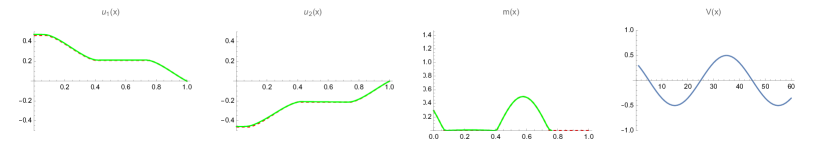
Figure 1: Graph of analytical (red dash) and numerical (green) solutions of density function, $m$, and two different value functions, $u_{1},u_{2}$, with zero current, $j_{0}$.

This example shows that there can be areas where $m$ vanishes. Because $u$ is invariant up to the addition of constants, it is always possible to have $u(1)=0$. Because the current is $0$, either the velocity is $0$ and $m\geq 0$ or the velocity is nonzero, and thus, $m$ vanishes.

2.1.2 The case $j_{0}>0$.

Analytical solution.

From the second equation of (2.1) and the initial condition of (2.2), we have

$$\begin{split}-m(x)u_{x}(x)=j_{0}.\end{split}$$

Because $j_{0}\neq 0$, $m$ cannot vanish. Thus, we can rewrite the latter identity as

$$u_{x}(x)=-\frac{j_{0}}{m(x)}.$$ (2.4)

Substituting this expression into the first equation of (2.1) and multiplying both sides by $m^{2}$, we get

$$m^{3}-V(x)m^{2}-\frac{j_{0}^{2}}{2}=0.$$ (2.5)

Solving this equation, we obtain a unique positive solution for $m$

$$\begin{split}m(x)=\begin{cases}\sqrt[3]{a(x)+b(x)}+\sqrt[3]{a(x)-b(x)}+\dfrac{V(x)}{3},&V>\gamma,\\ \dfrac{j_{0}^{2/3}}{2},&V(x)=\gamma,\\ \xi^{k_{0}}\sqrt[3]{a(x)+b(x)}+\dfrac{1}{\xi^{k_{0}}\sqrt[3]{a(x)+b(x)}}\left(\dfrac{V}{3}\right)^{2}+\dfrac{V}{3},&V(x)<\gamma,\end{cases}\end{split}$$

where $\xi$ is a complex cube root of $1$, $k_{0}$ is being chosen from $\{0,1,2\}$ in such a way that $m$ is positive, and

$$\begin{split}\gamma=-\dfrac{3}{2}j_{0}^{2/3},\quad a(x)=\left(\frac{V}{3}\right)^{3}+\left(\frac{j_{0}}{2}\right)^{2},\quad b(x)=\frac{j}{2}\sqrt{2\left(\frac{V}{3}\right)^{3}+\left(\frac{j_{0}}{2}\right)^{2}}.\end{split}$$

From relation (2.4), we see that $u_{x}$ is negative. Thus, from the first equation of (2.1), we get

$$\begin{split}u_{x}=-\sqrt{2(m-V(x))}.\end{split}$$

which gives us

$$\begin{split}u(x)=u(1)-\int_{x}^{1}\sqrt{2(m-V(x))}dx.\end{split}$$

Comparing numerical and analytical solutions.

Again, using ”Mathematica”, we numerically solve the variational problem (2.3), and in Figure 2, we compare the numerical result to the analytical solution.

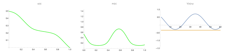
(a)

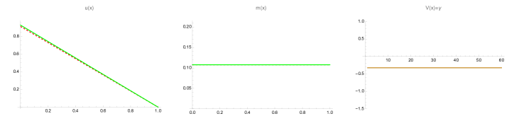
(b)

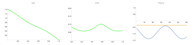
(c)

Figure 2: Graphs of analytical (red dash) and numerical (green) solutions of density function, $m$, and value function, $u$, with positive current, $j_{0}$, and different potential function $V(x)$. $(a)$ potential function is greater than the threshold $\gamma=-\frac{3}{2}j_{0}^{2/3}$, $(b)$ $V(x)=\gamma$ and $(c)$ $V(x)<\gamma$.

This example shows that in 1-dimension whenever the current is positive, the distribution function, $m$, is always positive regardless of the sign and amplitude of the potential function $V$.

2.2 A 2-dimensional example

Consider a square $\Omega=(0,1)\times(0,1)$. Set $V(x,y):=3e^{-\pi x}\cos(\pi y)-\frac{1}{2}\pi^{2}e^{-2\pi x}$. Then, the functions

$$\begin{split}\begin{cases}u(x,y)=e^{-\pi x}\sin(\pi y)\qquad\text{ and }\\ m(x,y)=3e^{-\pi x}[\cos(\pi y)]^{+}\end{cases}\end{split}$$

solve the MFG

$$\begin{split}\begin{cases}\left[\frac{\left|\nabla u(x,y)\right|^{2}}{2}+V(x,y)\right]^{+}=m&\text{ for }(x,y)\in\Omega,\\ -\operatorname*{div}(m\nabla u)=-\nabla m\cdot\nabla u-m\Delta u=0&\text{ for }(x,y)\in\Omega,\end{cases}\end{split}$$

under the following boundary conditions:

• Neumann–Dirichlet boundary conditions

  $$\begin{split}\begin{cases}-m\partial_{x}u(0,y)=3\pi\,\frac{\phantom{\small+}[\sin(2\pi y)]^{+}}{2}\quad(\geq 0)&\text{ for }y\in[0,1],\\ m\partial_{y}u(x,1)=0&\text{ for }x\in[0,1],\vspace{3mm}\\ u(1,y)\leq e^{-\pi}\sin(\pi y)&\text{ for }y\in[0,1],\\ u(x,0)\leq 0&\text{ for }x\in[0,1].\end{cases}\end{split}$$

• the contact-set conditions

  $$\begin{split}\begin{cases}m\partial_{x}u(1,y)\leq 0&\text{ if }u(1,y)=e^{-\pi}\sin(\pi y)\text{ for }y\in[0,1],\\ m\partial_{x}u(1,y)=0&\text{ if }u(1,y)<e^{-\pi}\sin(\pi y)\text{ for }y\in[0,1],\vspace{3mm}\\ -m\partial_{y}u(x,0)\leq 0&\text{ if }u(x,0)=0\text{ for }x\in[0,1],\\ -m\partial_{y}u(x,0)=0&\text{ if }u(x,0)<0\text{ for }x\in[0,1].\end{cases}\end{split}$$

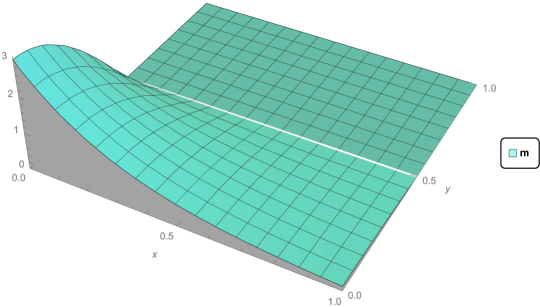
Figure 3: Graph of $m$.

Here, $u$ coincides with $\psi$ on the Dirichlet boundary, and, as the constraints require,

$$\begin{split}\begin{cases}m\partial_{x}u(1,y)=-3\pi e^{-2\pi}\,\frac{\phantom{\small+}[\sin(2\pi y)]^{+}}{2}\quad\leq 0&\text{ for }y\in[0,1],\\ -m\partial_{y}u(x,0)=-3\pi e^{-2\pi x}\,[\cos(\pi y)]^{+}\quad\leq 0&\text{ for }x\in[0,1].\end{cases}\end{split}$$

This example highlights several important features. Firstly, stationary MFGs may have empty regions, as is the case here where $m\equiv 0$ in $[0,1]\times[1/2,1]$. Secondly, it is not necessary that $u\equiv\psi$ on $\Gamma_{D}$. Although $u$ coincides with $\psi$ on the Dirichlet boundary in this example, by making $\psi$ larger where the flow at the Dirichlet part of the boundary is zero, we can show that one may only achieve the inequality ($u<\psi$) at the boundary. Thirdly, the free boundary $F_{m}:=\partial\{x\in\Omega\,:\,m(x)>0\}\cap\Omega$ can be expressed explicitly as $\{(x,1/2)\,:\,0<x<1\}$, with the normal vector given by $\nu=(0,1)$. Moreover, we have that

$$\begin{split}-\nabla u(x,1/2)\cdot\nu=-\partial_{y}u(x,1/2)=-\pi e^{-\pi x}\cos(\pi/2)=0.\end{split}$$

This shows that the current direction $\nabla u(x,y)$ is tangential to the free boundary $F_{m}$. We discuss this in more detail in Section 8.

2.3 A complex variable construction in two dimensions

Here, we present a method for generating examples of explicitly solvable MFGs of the form

$$\begin{split}\begin{cases}\left[\frac{\left|\nabla u(x,y)\right|^{2}}{2}+V(x,y)\right]^{+}=m^{1/q}&\text{ for }(x,y)\in\Omega,\\ -\operatorname*{div}(mDu)=-\nabla m\cdot\nabla u-m\Delta u=0&\text{ for }(x,y)\in\Omega.\end{cases}\end{split}$$ (2.6)

Consider a differentiable, complex-valued mapping $z=x+iy\longmapsto f(z)=u(x,y)+im(x,y)$, where $u$ and $m$ are real-valued functions. From the Cauchy-Riemann equations, we have

$$\begin{split}\begin{cases}\frac{\partial}{\partial x}u&=\frac{\partial}{\partial y}m\\ \frac{\partial}{\partial y}u&=-\frac{\partial}{\partial x}m.\end{cases}\end{split}$$

Thus, we have

$$\begin{split}\nabla u\cdot\nabla m=\frac{\partial}{\partial x}u\,\frac{\partial}{\partial x}m+\frac{\partial}{\partial y}u\,\frac{\partial}{\partial y}m=0.\end{split}$$

Because $f$ is differentiable, $u$ is harmonic; that is, $u$ solves $-\Delta u=0$. Then, $m$ and $u$ solve the continuity equation;

$$\begin{split}-\operatorname*{div}(mDu)=-Dm\cdot Du-m\Delta u=0.\end{split}$$ (2.7)

Then, we choose $V(x,y)$ to satisfy the first equation in (2.6). For example,

$$\begin{split}V(x,y)=m(x,y)^{1/q}-\frac{\left|\nabla u(x,y)\right|^{2}}{2}\end{split}$$

In general, $m$ may fail to be positive, which can be overcome by replacing $m$ with $\widetilde{m}:=(m)^{+}$ and setting, for example,

$$\begin{split}V(x,y)=\widetilde{m}(x,y)^{1/q}-\frac{\left|\nabla u(x,y)\right|^{2}}{2}.\end{split}$$

Then, we have

$$\begin{split}\begin{cases}\left[\frac{\left|\nabla u(x,y)\right|^{2}}{2}+V(x,y)\right]^{+}=\widetilde{m}^{1/q}&\text{ for }(x,y)\in\Omega,\\ -\operatorname*{div}(\widetilde{m}Du)=0&\text{ for }(x,y)\in\Omega.\end{cases}\end{split}$$

The first equation holds in the strong sense (a.e. in $\Omega$), while the second equation holds in the sense of distributions.

3 Notation and assumptions

In later sections, we investigate the behavior of solutions in the nonempty region, where $m>0$, and around the free boundary associated with $m$. We use the following notation.

Definition 3.1.

For a function $\mu:\Omega\to\mathbb{R}$, the free boundary of $\mu$ is

$$\begin{split}F_{\mu}:=\partial\{x\in\Omega\,:\,\mu>0\}\cap\Omega.\end{split}$$ (3.1)

The relation between Problem 1 and Problem 2 is dependent on the relationship between $G$ and $g$. While it is possible to define $G$ in terms of $g$, it is more practical to do the opposite. This is because it is simpler to explain and motivate our assumptions in terms of $G$.

Definition 3.2.

Let $G:\mathbb{R}\to\mathbb{R}$ be a non-decreasing, convex function. The pseudo-inverse $g:G^{\prime}(\mathbb{R})\to\mathbb{R}_{0}^{+}$ of $G^{\prime}$ is

$$\begin{split}g(\mu):=((G^{\prime})^{-1})(\mu)=\max\{z\in\mathbb{R}\,:\,G^{\prime}(z)=\mu\}.\end{split}$$ (3.2)

Remark 3.3.

Our definition of pseudo-inverse slightly deviates from the standard one. Usually, we would set $(G^{\prime})^{-1}(\mu)=\max\{z\in\mathbb{R}^{+}\,:\,G^{\prime}(z)\geq\mu\}$. However, the two definitions are equivalent when $G^{\prime}$ is continuous. Moreover, our definition gives us directly that

$$\begin{split}G^{\prime}(g(m))\equiv G^{\prime}((G^{\prime})^{-1}(m))=m,\end{split}$$

which is needed in some of our proofs.

3.1 Assumptions on problem data

To study the variational problem, we need the following conditions on $G$.

Assumption 1.

For $G:\mathbb{R}\to\mathbb{R}$, the following holds.

1. $G\in C^{1}(\mathbb{R})$.

2. $G$ is coercive, convex, and non-decreasing.

3. There exist $\alpha>1$ and a constant $C>0$ such that, for all $z\in\mathbb{R}$, large enough,

   $$\begin{cases}\dfrac{|z|^{\alpha}}{C}-C\leq G(z)\leq C(|z|^{\alpha}+1),\\ |G^{\prime}(z)|\leq C(|z|^{\alpha-1}+1).\end{cases}$$

4. There exists a constant $C>0$, such that, for all $z\in\mathbb{R}$, large enough,

   $$G^{\prime}(z)z\geq-C.$$

Remark 3.4.

Since $G$ is a non-decreasing, convex function on $\mathbb{R}$, there exists at most a value $z_{1}\in\mathbb{R}$, such that $G$ is constant on an interval $(-\infty,z_{1}]$, after that point $G$ is increasing. That is, $G^{\prime}(z)=0$ on $[-\infty,z_{1}]$ and $G^{\prime}(z)>0$, for all $z>z_{1}$.

Notice that because $G^{\prime}$ may not be strictly increasing, i.e., it may be constant in some regions, its pseudo-inverse $g$ can be discontinuous. However, $g$ is always strictly increasing.

The conditions on $G$, in Assumption 1, are implied by the following conditions on the coupling $g$ in the MFG (Problem 1).

Assumption 2.

For $g:\mathbb{R}_{0}^{+}\to\mathbb{R}$, the following hold.

1. $g\in C^{1}(\mathbb{R}_{0}^{+})$.

2. $g$ is non-negative and increasing.

3. There exist $\alpha>1$ and constant $C>0$ such that, for $z\in\mathbb{R}_{0}^{+}$, large enough,

   $$\dfrac{|z|^{\frac{1}{\alpha-1}}}{C}\leq g(z)\leq C(|z|^{\frac{1}{\alpha-1}}+1).$$

Remark 3.5.

The first point in the preceding assumption, in particular, requires that $0\in G^{\prime}(\mathbb{R})$, i.e., since $G$ is convex, then $G$ has a minimizer.

Remark 3.6.

The conditions on $g$, in Assumption 2, imply that for all $\delta>0$, there exists a constant $C_{\delta}>0$, s.t.

$$\begin{split}\int_{\Omega}mdx,\;\int_{\Omega}g(m)dx\leq\delta\int_{\Omega}mg(m)dx+C_{\delta}.\end{split}$$

This remark is used later in the proof of Proposition 5.1.

Assumption 3.

For $H:\overline{\Omega}\times\mathbb{R}^{d}\to\mathbb{R}$, the following holds.

1. $H\in C^{2}(\overline{\Omega}\times\mathbb{R}^{d})$.

2. $H$ is bounded from below.

3. For all $x\in\Omega$, the map $p\mapsto H(x,p)$ is uniformly convex.

4. There exist $\beta>1$ and positive constant $C>0$ such that, for all $(x,p)\in\Omega\times\mathbb{R}^{d})$,

   $$\begin{split}\begin{cases}\dfrac{|p|^{\beta}}{C}-C\leq H(x,p)\leq C(|p|^{\beta}+1),\\ |D_{x}H(x,p)|\leq C(|p|^{\beta}+1),\\ |D_{p}H(x,p)|\leq C(|p|^{\beta-1}+1),\end{cases}\end{split}$$

5. and $H$ satisfies the lower bound

   $$\begin{split}-H(x,p)+D_{p}H(x,p)p\geq\dfrac{|p|^{\beta}}{C}-C.\end{split}$$

Notice that, due to our assumptions on $G$ and $H$, the map $p\mapsto G(H(x,p)+V(x))$ is convex and bounded below. This map appears in the integrand of the cost functional (1.6). This convexity and lower boundedness are (mathematically) reasonable assumptions for the existence of minimizers for (1.6).

In what follows, if $\tau$ is an exponent parameter, then $\tau^{\prime}$ is its conjugate exponent, i.e. $\dfrac{1}{\tau}+\dfrac{1}{\tau^{\prime}}=1$. Because $j$ is an incoming flow of agents, we require it to be non-negative and satisfy suitable integrability conditions.

Assumption 4.

The incoming flow satisfies $j\in L^{\beta^{\prime}}(\Gamma_{N})$ and $j(s)\geq 0$.

Our last assumption requires some minimal regularity on the exit costs and, for convenience, assumes these are the traces of a function defined on the whole set $\Omega$.

Assumption 5.

The exit cost satisfies $\psi\in W^{1,\gamma}(\Omega)$.

3.2 Model Hamiltonian and Energy Gauge

Here, we give an example of $H$ and $G$ that satisfies our assumptions. Let $b(\cdot)$ be a smooth function with values in some bounded interval $(\delta,\frac{1}{\delta})$, for $\delta>0$, and $a$ be a positive constant. Define

$$\begin{split}&H(x,p)=b(x)[(|p|^{2}+1)^{\frac{\beta}{2}}-1]+\sin(|x|^{2}),\quad G(z)=a(z+1)^{\alpha}.\end{split}$$ (3.3)

The domain of $G$ is $[-1,\infty)$ and is extended by $0$ for $z<-1$, so that our definition is compatible with the assumptions.

The functions $H$ and $G$ have the necessary regularity. The rest of the assumptions are verified in what follows.

3.2.1 Assumptions on the coupling

First, we verify that the assumptions on the coupling term, $G$, hold.

1. the coercivity is clear since $\alpha>1$; so $G(z)/z\to\infty$ as $z\to\infty$. The function $G$ is non-decreasing on $[-1,\infty)$ and thus in $\mathbb{R}$. It is also convex since $G^{\prime\prime}(z)=a\alpha(\alpha-1)(z+1)^{\alpha-2}\geq 0$.

2. For $z>0$, we have

   $$\begin{split}az^{\alpha}\leq G(z)=a(z+1)^{\alpha}\leq 2^{\alpha-1}a(z^{\alpha}+1),\end{split}$$

   and

   $$\begin{split}|G^{\prime}(z)|=|a\alpha(z+1)^{\alpha-1}|\leq a\alpha 2^{\alpha-1}(z^{\alpha-1}+1).\end{split}$$

3. We have

   $$\begin{split}G^{\prime}(z)z>-\alpha a.\end{split}$$

3.2.2 Assumptions on the Hamiltonian

Now, we check that the assumptions on the Hamiltonian, $H$, hold.

1. It is clear that $H$ is bounded below since $b[(|p|^{2}+1)^{\frac{\beta}{2}}-1]+\sin(|x|^{2})\geq b[(0+1)^{\frac{\beta}{2}}-1]-1=-1$.

2. The strict convexity of $H$ follows from the fact that, for every nonzero vector $v\in\mathbb{R}^{d}$, we have

   $$\begin{split}v^{*}D_{pp}Hv&=v^{*}\left[p^{*}p\,b(x)\beta(\beta-2)(|p|^{2}+1)^{\frac{\beta}{2}-2}+b(x)\beta(|p|^{2}+1)^{\frac{\beta}{2}-1}I\right]v\\ &=b(x)\beta(|p|^{2}+1)^{\beta/2-2}\left[(\beta-2)|p\cdot v|^{2}+(|p|^{2}+1)|v|^{2}\right]\\ &=b(x)\beta(|p|^{2}+1)^{\beta/2-2}\left[(\beta-1)|p\cdot v|^{2}+|v|^{2}+(|v|^{2}|p|^{2}-|p\cdot v|^{2})\right]\\ &\geq\delta\beta(|p|^{2}+1)^{\beta/2-2}\left[0+|v|^{2}+0\right]>0.\end{split}$$

3. $H$ has a polynomial growth, in $p$, of order $\beta$ since

   $$\begin{split}\delta(|p|^{2})^{\beta/2}-\frac{1}{\delta}\,\,\leq\,\,b(x)[(|p|^{2}+1)^{\beta/2}-1]\,\,\leq\,\,\frac{1}{\delta}\,2^{\beta/2}\,(|p|^{\beta}+1)-\delta.\end{split}$$

   Additionally, $|D_{x}H|$ and $|D_{p}H|$, as functions in $p$, are of orders $\beta$ and $\beta-1$, respectively; indeed,

   $$\begin{split}|D_{x}H(x,p)|&\leq|Db|[(|p|^{2}+1)^{\beta/2}-1]+2|x|\,\,\leq\,\,||Db||_{\infty}\,2^{\beta/2}\,(|p|^{\beta}+1)+||x||_{\infty,\Omega},\\ |D_{p}H(x,p)|&=b(x)\beta(|p|^{2}+1)^{\frac{\beta}{2}-1}|p|\,\,\leq\,\,b(x)\beta(|p|^{2}+1)^{\frac{\beta}{2}-\frac{1}{2}}\,\,\leq\,\,\frac{\beta}{\delta}\,2^{(\beta-1)/2}\,(|p|^{\beta-1}+1).\end{split}$$

4 A Variational Formulation of the MFG

In this section, we show that (1.1) is the Euler–Lagrange equation of Problem 2, and that (1.2) are the natural boundary conditions. We also include a subsection explaining what it means for a pair $(m,u)$ to solve (1.1)-(1.2), which is motivated by the derivation of the MFG from its variational formulation.

4.1 Variational Formulation of the MFG

Let $u\in\mathcal{D}$ be a minimizer of (1.6), and set $m(x):=G^{\prime}(H(x,Du))$. For the sake of clarity, we assume that $(m,u)\in W^{1,\alpha^{\prime}}(\Omega)\times W^{2,\gamma}(\Omega)$. However, it is worth noting that we can relax this requirement without compromising the rigor of the derivation (see Remark 4.2 below). We divide the derivation into two steps.

Step 1 (Interior equations and Neumann boundary condition): Let $v\in C^{\infty}(\Omega)$ be an arbitrary function such that $v\equiv 0$ on $\Gamma_{D}$, and define the function $i(\varepsilon)=\mathcal{I}[u+\varepsilon v]$. Since $u$ is a solution to the minimization problem, we have $i(0)\leq i(\epsilon)$. From basic calculus, we see that $i^{\prime}(0)=0$. This implies that

$$\begin{split}0&=\frac{d}{d\varepsilon}\mathcal{I}[u+\varepsilon v]|_{\varepsilon=0}\\ &=\frac{d}{d\varepsilon}\left(\int_{\Omega}G\left(H(x,Du+\varepsilon Dv)\right)dx-\int_{\Gamma_{N}}j(u+\varepsilon v)\,ds\right)\Big{|}_{\varepsilon=0}\\ &=\int_{\Omega}G^{\prime}\left(H(x,Du)\right)D_{p}H(x,Du)\cdot Dvdx-\int_{\Gamma_{N}}jv\,ds\\ &=-\int_{\Omega}\operatorname*{div}(mD_{p}H(x,Du))v+\int_{\Gamma_{N}}\left(mD_{p}H(x,Du)\cdot\nu-j\right)v\,ds.\end{split}$$

Since $v$ is arbitrary, we see that

$$\begin{cases}G^{\prime}(H(x,Du))=m&\text{ for all }x\in\Omega,\\ -\operatorname*{div}(mD_{p}H(x,Du))=0&\text{ for all }x\in\Omega,\\ mD_{p}H(x,Du)\cdot\nu=j&\text{ for all }x\in\Gamma_{N}.\end{cases}$$ (4.1)

Remark 4.1.

We can derive under the integral because we have the proper growth and convexity for $G$ and $H$. In fact, for some constant $\overline{C}$, we can show that

$$\begin{split}\left|\frac{G\left(H(x,Du+\varepsilon Dv)\right)-G\left(H(x,Du)\right)}{\epsilon}\right|\leq\overline{C}\left[\left|Du\right|^{\gamma-1}+\varepsilon^{\gamma-1}\left|Dv\right|^{\gamma-1}\right].\end{split}$$

By the dominated convergence theorem, we can exchange the limit ($\lim_{\epsilon\to 0}$) and the integral; hence, we can derive under the integral.

Step 2 (The first Dirichlet boundary condition): Here, we use here, the same method with a different choice of $v$. Indeed, let $v$ be a function in $C^{\infty}(\overline{\Omega})$ satisfying that $v(x)\leq 0$ for all $x\in\Gamma_{D}$. Then, for every $\epsilon\geq 0$, we have that $u+\epsilon v$ is in the admissible set $\mathcal{D}$. Hence, restricted to $[0,+\infty)$, the map $i(\epsilon):=\mathcal{I}[u+\epsilon v]$ attains a minimum at $0$. Thus, $i^{\prime}(0)\geq 0$ and

$$0 \leq\int_{\Omega}G^{\prime}(H(x,Du))D_{p}H(x,Du)Dv\,dx-\int_{\Gamma_{N}}jv\,ds$$

$$=-\int_{\Omega}\operatorname*{div}\left(mD_{p}H(x,Du)\right)v\,dx+\int_{\Gamma_{N}}(mD_{p}H(x,Du)\cdot\nu-j)\,v\,ds+\int_{\Gamma_{D}}vmD_{p}H(x,Du)\cdot\nu\,ds.$$

Using (4.1), we have

$$\begin{split}0\leq\int_{\Gamma_{D}}vmD_{p}H(x,Du)\cdot\nu\,ds\end{split}$$

for all smooth functions $v$ satisfying $v\leq 0$ on $\Gamma_{D}$. Thus, we have

$$\begin{split}mD_{p}H(x,Du)\cdot\nu\leq 0\qquad\text{on }\Gamma_{D}.\end{split}$$ (4.2)

Step 3 (The second Dirichlet boundary condition): We use, once more, the same method with a different choice of perturbation function. Let $v\in C^{\infty}(\overline{\Omega})$ be arbitrary and define $i(\epsilon):=\mathcal{I}[u+\epsilon(\psi-u)v]$ for all $\epsilon$ such that $\sup_{\Gamma_{D}}\left|\epsilon v\right|<1$. Notice first that $u+\epsilon v(\psi-u)\leq u+(\psi-u)=\psi$ on $\Gamma_{D}$; hence, $u+\epsilon v(\psi-u)$ is in the admissible set $\mathcal{D}$. Moreover, $i(\cdot)$ attains a minimum at $0$. Thus, $i^{\prime}(0)=0$. Using an argument similar to the first two steps, we obtain

$$0 =-\int_{\Omega}\operatorname*{div}\left(mD_{p}H(x,Du)\right)v(\psi-u)\,dx+\int_{\Gamma}v(\psi-u)\,mD_{p}H(x,Du)\cdot\nu\,ds-\int_{\Gamma_{N}}j\,v(\psi-u)\,ds$$

$$=\int_{\Gamma_{D}}v(\psi-u)\,mD_{p}H(x,Du)\cdot\nu\,ds$$

for all smooth functions $v$. Thus, we have

$$\begin{split}(\psi-u)mD_{p}H(x,Du)\cdot\nu\,ds=0\qquad\text{on }\Gamma_{D}.\end{split}$$ (4.3)

Next, we define $g$ to be the generalized inverse of $G^{\prime}$ according to Definition 3.2. Finally, by combining (4.1), (4.2), and (4.3), we obtain that the MFG (1.1)-(1.2) is the Euler-Lagrange equation for the variational problem.

Remark 4.2.

While the derivation of the Euler-Lagrange equation in Step 1 is rigorous for an arbitrary $u\in W^{1,\gamma}(\Omega)$, we assume more regularity on $(m,u)$ so that $mD_{p}H(x,Du)$ possesses a trace in the usual sense. However, as we discuss in Section A.3 of the appendix, the function $m(\cdot)D_{p}H(\cdot,Du(\cdot))$ belongs to a function space that is equipped with a Neumann trace operator; that is, $m(x)D_{p}H(x,Du(x))\cdot\nu(x)$ is well-defined in $\Gamma$.

4.2 Definition of weak solution

Our definition of weak solution is similar to the one employed in [CG15]. The only difference with our definition is that we have mixed boundary conditions, which we request to be satisfied in the trace sense. More precisely, we define a weak solution as follows.

Definition 4.3.

A weak solution to Problem 1 is a pair of functions $(m,u)\in L^{\alpha^{\prime}}(\Omega)\times W^{1,\gamma}(\Omega)$ that satisfies

1. the boundary condition (1.2) in the trace sense at the Dirichlet boundary, and in the Neumann (or normal) trace sense at the Neumann boundary (see, Appendix A.3),

2. $m\geq 0$ and $mD_{p}H(x,Du)\in L^{1}(\Omega)$,

3. the first equation of (1.1) holds in the following sense:

   $$\begin{split}H(x,Du)=g(m),\quad\text{ a.e. in }\{m>0\},\end{split}$$

   and

   $$\begin{split}H(x,Du)\leq g(m),\quad\text{ a.e. in }\Omega,\end{split}$$

4. the second equation of (1.1) holds in the sense of distributions.

Remark 4.4.

While (distributional) derivatives of functions in $W^{1,\gamma}$ may not have traces on $\partial\Omega$, we show in Appendix A.3 that $mD_{p}H(x,Du)\cdot\nu$ is defined on $\partial\Omega$ in the sense of traces, which we call the Neumann (normal) trace.

5 Formal estimates

This section discusses formal estimates for our problem. We begin by introducing first-order apriori estimates, which are well-known in MFGs, and show that our boundary conditions are compatible with these estimates.

Proposition 5.1.

Suppose that Assumptions 2–5 hold. Then, there exists a positive constant $C_{0}>0$, depending only on the data of Problem 1 ($\psi,j,\alpha,\beta,\Omega$), such that for any classical solution $(m,u)$ to Problem 1, we have

$$\int_{\Omega}mg(m)+\dfrac{(m+1)|Du|^{\beta}}{C}dx\leq C_{0}.$$ (5.1)

Proof.

Multiplying the first equation in (1.1) by $(m-1)$ and the second equation by $(u-\psi)$, adding and integrating over $\Omega$, and then integrating by parts and taking into consideration the boundary conditions (1.2), we get

$$\int_{\Omega}mg(m)+m(-H(x,Du) +D_{p}H(x,Du)Du)+H(x,Du)dx=$$ (5.2)

$$= \int_{\Omega}g(m)+mV-V+mD_{p}H(x,Du)D\psi dx+\int_{\Gamma_{N}}j(u-\psi)ds.$$

Using Young’s inequality, Assumption 3, and the non-negativity of $m$, we get the estimates

$$\int_{\Omega}m(-H(x,Du)+D_{p}H(x,Du)Du)+H(x,Du)dx\geq\int_{\Omega}(m+1)\dfrac{|Du|^{\beta}}{C}dx-C\int_{\Omega}mdx-C,$$ (5.3)

and

$$\int_{\Omega}mD_{p}H(x,Du)D\psi dx\leq C\int_{\Omega}m|Du|^{\beta-1}dx+C\int_{\Omega}mdx\leq\int_{\Omega}\epsilon m|Du|^{\beta}dx+C\int_{\Omega}mdx+C.$$ (5.4)

Additionally, from Assumption 2, we have

$$\int_{\Omega}m\,dx\,,\,\int_{\Omega}g(m)dx\leq\delta\int_{\Omega}mg(m)dx+C_{\delta}.$$ (5.5)

Now, we want to obtain a bound for $\int_{\Gamma_{N}}j(u-\psi)\,dx$ in the form

$$\int_{\Gamma_{N}}j(u-\psi)ds\leq C\|Du\|_{L^{\beta}}+C\leq\int_{\Omega}\epsilon|Du|^{\beta}dx+C.$$ (5.6)

We use Assumption 4, the trace theorem, and Poincaré inequality to establish this estimate. Because $j\geq 0$, we have

$$\begin{split}\int_{\Gamma_{N}}j(u-\psi)\leq\int_{\Gamma_{N}}j(u-\psi)^{+}.\end{split}$$

Using Hölder’s inequality and that $(u-\psi)^{+}=0$ on $\Gamma_{D}$, we obtain

$$\begin{split}{\int_{\Gamma_{N}}j(u-\psi)^{+}}&\leq\left(\int_{\Gamma_{N}}j^{\beta^{\prime}}\right)^{1/\beta^{\prime}}\left(\int_{\Gamma_{N}}\left|(u-\psi)^{+}\right|^{\beta}\right)^{1/\beta}=\left(\int_{\Gamma_{N}}j^{\beta^{\prime}}\right)^{1/\beta^{\prime}}\left(\int_{\Gamma}\left|(u-\psi)^{+}\right|^{\beta}\right)^{1/\beta}.\end{split}$$

Moreover, from the trace theorem, we have

$$\begin{split}\left\lVert(u-\psi)^{+}\right\rVert_{L^{\beta}(\Gamma)}&\leq C\left[\left\lVert(u-\psi)^{+}\right\rVert_{L^{\beta}(\Omega)}+\left\lVert D(u-\psi)^{+}\right\rVert_{L^{\beta}(\Omega)}\right].\end{split}$$

Since $(u-\psi)^{+}=0$ on $\Gamma_{D}$, and $|\Gamma_{D}|>0$, Poincaré inequality gives us

$$\begin{split}\int_{\Omega}\left|(u-\psi)^{+}\right|^{\beta}\leq C\int_{\Omega}{\left|D(u-\psi)^{+}\right|^{\beta}}\leq C\int_{\Omega}{\left|D(u-\psi)\right|^{\beta}}.\end{split}$$

Combining the inequalities above, we obtain

$$\begin{split}\int_{\Gamma_{N}}j(u-\psi)\,ds&\leq C\left\lVert D(u-\psi)\right\rVert_{L^{\beta}(\Omega)}\leq C\left\lVert Du\right\rVert_{L^{\beta}(\Omega)}+C\left\lVert D\psi\right\rVert_{L^{\beta}(\Omega)}.\end{split}$$

Finally, taking proper values for $\epsilon$ and $\delta$ in estimates (5.3)–(5.6), and combining them with (5.2), we get the desired result. ∎

From this estimate, we obtain the following regularity for $m$.

Corollary 5.2.

Under the assumptions of the previous proposition, suppose the pair $(m,u)$ solves Problem 1. Then, $m\in L^{\alpha^{\prime}}(\Omega)$ and $g(m)\in L^{\alpha}(\Omega)$.

Proof.

Using Assumption 2, we have

$$\begin{split}\int_{\Omega}m^{\alpha^{\prime}}\,dx=\int_{\Omega}m\,m^{\frac{1}{\alpha-1}}\,dx\leq C\int_{\Omega}mg(m)\,dx\leq C<\infty,\end{split}$$

$$\begin{split}\int_{\Omega}g^{\alpha}(m)\,dx\leq C\int_{\Omega}m^{\frac{\alpha}{\alpha-1}}\,dx+C\leq\int_{\Omega}m^{\alpha^{\prime}}\,dx+C\leq C<\infty.\end{split}$$

∎

Corollary 5.3.

Under the assumptions of the previous proposition, suppose the pair $(m,u)$ solves Problem 1. If $j(s)>0$ on a subset of $\Gamma_{N}$ of strictly positive measure, then $u\in W^{1,\gamma}(\Omega)$.

Proof.

The first equation of (1.1) and Corollary 5.2 yield $H\in L^{\alpha}(\Omega)$. By Assumption 3, we have

$$\int_{\Omega}|Du|^{\gamma}\,dx= \int_{\Omega}\left(|Du|^{\beta}\right)^{\alpha}\,dx\leq\int_{\Omega}C^{\alpha}\left(H(x,Du)+C\right)^{\alpha}\,dx\leq$$

$$\leq 2^{\alpha-1}C^{\alpha}\int_{\Omega}|H(x,Du)|^{\alpha}\,dx+C<\infty.$$

Thus, we get $Du\in L^{\gamma}(\Omega)$.

It remains to show that $u\in L^{\gamma}(\Omega)$. To this end, we integrate the second equation in (1.1), and use the first boundary condition in (1.2) to get

$$\begin{split}0=-\int_{\Omega}\operatorname*{div}(mD_{p}H(x,Du))dx=-\int_{\Gamma_{N}}j(s)ds-\int_{\Gamma_{D}}mD_{p}H(x,Du)\nu ds,\end{split}$$

$$\begin{split}\int_{\Gamma_{D}}mD_{p}H(x,Du)\nu ds=-\int_{\Gamma_{N}}j(s)ds\neq 0.\end{split}$$

The second boundary condition in (1.2), that is $mD_{p}H(x,Du)\nu\leq 0$, yields that there is a subset $\Gamma_{D}^{0}\subset\Gamma_{D}$ with positive measure, such that

$$\begin{split}mD_{p}H(x,Du)\nu<0,\quad\mbox{ on }\Gamma_{D}^{0}.\end{split}$$

Finally, from the complementary condition in (1.2), we get

$$\begin{split}(u-\psi)=0,\quad\mbox{ on }\Gamma_{D}^{0}.\end{split}$$

Now, Poincaré inequality for the function $(u-\psi)$ gives us

$$\int_{\Omega}\left|u\right|^{\gamma}= \int_{\Omega}\left|(u-\psi)+\psi\right|^{\gamma}\leq C\int_{\Omega}\left|(u-\psi)\right|^{\gamma}+\left|\psi\right|^{\gamma}\leq$$

$$\leq C\int_{\Omega}{\left|D(u-\psi)\right|^{\gamma}}+C\int_{\Omega}\left|\psi\right|^{\gamma}\leq C\int_{\Omega}{\left|Du\right|^{\gamma}}dx+C\int_{\Omega}{\left|D\psi\right|^{\gamma}}+\left|\psi\right|^{\gamma}dx<\infty.$$

This completes the proof. ∎

6 The variational problem

This section establishes a lower bound on the functional from the variational problem. Then, we prove the existence of a minimizer. Subsequently, we examine the correspondence between problems 1 and 2. Finally, we present additional regularity estimates and examine the uniqueness of a solution.

6.1 Estimates on the cost functional

We first establish the following lemma to show that the cost functional is bounded below.

Lemma 6.1.

With the Assumptions 4 and 5, suppose that $w\in W^{1,\gamma}(\Omega)$ is an admissible function in Problem 2. Then, there is a constant $C$, depending only on $j$, $\Omega$, $\Gamma_{N}$, $\Gamma_{D}$, $\gamma$, and $\psi$, such that

$$\begin{split}\int_{\Gamma_{N}}jw\leq C+C\left(\int_{\Omega}\left|Dw\right|^{\gamma}\right)^{1/\gamma}.\end{split}$$

Proof.

The proof is similar to that of Proposition 5.1. To establish this estimate, we use the trace theorem and Poincaré inequality. Because $j\geq 0$, we have

$$\begin{split}\int_{\Gamma_{N}}j(w-\psi)\leq\int_{\Gamma_{N}}j(w-\psi)^{+}.\end{split}$$ (6.1)

Using Hölder’s inequality and that $(u-\psi)^{+}=0$ on $\Gamma_{D}$, we obtain

$$\begin{split}{\int_{\Gamma_{N}}j(w-\psi)^{+}}&\leq\left(\int_{\Gamma_{N}}j^{\gamma^{\prime}}\right)^{1/\gamma^{\prime}}\left(\int_{\Gamma_{N}}\left|(w-\psi)^{+}\right|^{\gamma}\right)^{1/\gamma}=\left(\int_{\Gamma_{N}}j^{\gamma^{\prime}}\right)^{1/\gamma^{\prime}}\left(\int_{\Gamma}\left|(w-\psi)^{+}\right|^{\gamma}\right)^{1/\gamma}.\end{split}$$ (6.2)

Moreover, from the trace theorem, we have that

$$\begin{split}\left\lVert(w-\psi)^{+}\right\rVert_{L^{\gamma}(\Gamma)}&\leq C\left[\left\lVert(w-\psi)^{+}\right\rVert_{L^{\gamma}(\Omega)}+\left\lVert D(w-\psi)^{+}\right\rVert_{L^{\gamma}(\Omega)}\right].\end{split}$$

Since $(w-\psi)^{+}=0$ on $\Gamma_{D}$, and $|\Gamma_{D}|>0$, Poincaré inequality gives us that

$$\begin{split}\int_{\Omega}\left|(w-\psi)^{+}\right|^{\gamma}\leq C\int_{\Omega}{\left|D(w-\psi)^{+}\right|^{\gamma}}\leq C\int_{\Omega}{\left|D(w-\psi)\right|^{\gamma}}.\end{split}$$ (6.3)

Combining the inequalities above, we obtain

$$\begin{split}\int_{\Gamma_{N}}jw-\int_{\Gamma_{N}}j\psi&\leq C\left\lVert D(w-\psi)\right\rVert_{L^{\gamma}(\Omega)}\leq C\left\lVert Dw\right\rVert_{L^{\gamma}(\Omega)}+C\left\lVert D\psi\right\rVert_{L^{\gamma}(\Omega)}.\end{split}$$

This establishes our claim. ∎

Next, we give a lower bound for the cost functional.

Proposition 6.2.

Under Assumptions 1-5, let $w\in W^{1,\gamma}(\Omega)$ be an admissible function in Problem 2. Then, there is a constant $C$, depending only on $j$, $\Omega$, $\Gamma_{N}$, $\Gamma_{D}$, $\gamma$, and $\psi$, such that

$$\begin{split}\mathcal{I}[w]\geq C.\end{split}$$

Proof.

From Assumptions 1-5, we have that

$$\begin{split}G(H(x,Dw))\geq\widetilde{C}\left|Dw\right|^{\gamma}-\widetilde{C}.\end{split}$$ (6.4)

Also, due to Lemma 6.1, we have that

$$\begin{split}-\int_{\Gamma_{N}}jw\,ds\geq-C\left(\int_{\Omega}\left|Dw\right|^{\gamma}\right)^{1/\gamma}-C.\end{split}$$ (6.5)

Moreover, for $\xi\geq 0$, we can bound the function $\Xi(\xi):=\widetilde{C}\xi^{\gamma}-C\xi$ from below by a constant, $\overline{C}$, that depends only on $\widetilde{C}$, $C$. Combining the equations (6.4) and (6.5), we obtain

$$\begin{split}\mathcal{I}[w]&=\int_{\Omega}G(H(x,Dw))dx-\int_{\Gamma_{N}}jw\,ds\\ &\geq\widetilde{C}\int_{\Omega}\left|Dw\right|^{\gamma}-C\left(\int_{\Omega}\left|Dw\right|^{\gamma}\right)^{1/\gamma}-\widetilde{C}-C\geq\overline{C}-\widetilde{C}-C.\end{split}$$

This concludes the proof. ∎

Remark 6.3.

If we select $w\equiv\psi$, we have

$$\begin{split}\inf_{w\in\mathcal{D}}\mathcal{I}[w]\leq\mathcal{I}[\psi]\leq C\end{split}$$

for some constant $C$ that depends only on $\alpha$, $V$, and the geometry of $\Omega$. Thus, $\inf_{w\in\mathcal{D}}\mathcal{I}[w]$ is bounded above.

6.2 On the existence of a minimizer

Here, we use the estimates on the cost functional to show the existence of a minimizer for the variational problem.

Proof of Theorem 1.1.

Let $\{w_{n}\}\in\mathcal{D}$ be a minimizing sequence. From the proof of Lemma 6.1, we see that there is a constant $C>0$, independent of $n$, for which

$$\begin{split}\int_{\Omega}|Dw_{n}(x)|^{\gamma}ds-C\left(\int_{\Omega}|Dw_{n}(x)|^{\gamma}ds\right)^{1/\gamma}\leq C.\end{split}$$

Consequently,

$$\begin{split}\int_{\Omega}|Dw_{n}(x)|^{\gamma}ds\leq C\end{split}$$

for some positive constant $C$ independent of $n$ (and possibly different from the one above). Therefore, by using Poincaré inequality (in a similar manner to the proof of Lemma 6.1), we obtain that

$$\begin{split}\|w_{n}\|_{W^{1,\gamma}(\Omega)}\leq C.\end{split}$$

Next, notice that $\gamma>1$. Hence, $W^{1,\gamma}(\Omega)$ is a reflexive Banach space. Therefore, every bounded sequence in $W^{1,\gamma}(\Omega)$ (in particular $\{w_{n}\}$) is weakly precompact; that is, there exists a subsequence that converges weakly to a function $u\in W^{1,\gamma}(\Omega)$.

What remains now is to show that

$$\begin{split}\begin{cases}u\in\mathcal{D},\\ \displaystyle\liminf_{n\to\infty}\mathcal{I}[w_{n}]\geq\mathcal{I}[u].\end{cases}\end{split}$$

To this end, consider

$$\mathcal{I}[w_{n}]= \int_{\Omega}G(H(x,Dw_{n}))dx-\int_{\Gamma_{N}}jw_{n}ds$$

$$\geq \int_{\Omega}G(H(x,Du))dx-\int_{\Gamma_{N}}juds$$

$$+\int_{\Omega}G^{\prime}(H(x,Du))D_{p}H(x,Du)(Dw_{n}-Du)dx-\int_{\Gamma_{N}}j(w_{n}-u)ds.$$

Because $j\in L^{\gamma^{\prime}}(\Gamma_{N})$ and $G^{\prime}(H(\cdot,Du))D_{p}H(\cdot,Du)\in L^{\gamma^{\prime}}(\Omega)$, we have

$$\begin{split}\int_{\Gamma_{N}}j(w_{n}-u)ds\to 0,\end{split}$$

and

$$\begin{split}\int_{\Omega}G^{\prime}(H(x,Du))D_{p}H(x,Du)(Dw_{n}-Du)dx\to 0.\end{split}$$

It remains to show that $u\in\mathcal{D}$. Since $w_{n}\rightharpoonup u$ in $W^{1,\gamma}(\Omega)$, we have

$$\begin{split}\lim_{n\to\infty}\int_{\Gamma_{D}}f(w_{n}-\psi)ds=\int_{\Gamma_{D}}f(u-\psi)ds,\end{split}$$

for every $f\in L^{\gamma^{\prime}}(\Gamma_{D})$. Taking $f>0$, we conclude

$$\begin{split}\int_{\Gamma_{D}}f(u-\psi)ds\leq 0.\end{split}$$

Therefore, $u\leq\psi$ on $\Gamma_{D}$. ∎

6.3 First-order estimates

In this subsection, we establish several estimates that show a better regularity for solutions of the MFG. These estimates guarantee the applicability of some of our results (e.g., Neumann trace theorem in the appendix).

Lemma 6.4.

Let $u$ solve Problem 2 and $m=G^{\prime}(H(x,Du))$. Then, there exists a constant $C$, depending directly on the data of the problem, such that

$$\begin{split}m\leq C\left|Du\right|^{\beta(\alpha-1)}+C.\end{split}$$

Proof.

Since the pair $(m,u)$ is a solution to Problem 1, we have that

$$\begin{split}m=G^{\prime}(g(m))=G^{\prime}(H(x,Du)).\end{split}$$

Subsequently, we have

$$\begin{split}m=G^{\prime}(H(x,Du))&\leq C|H(x,Du)|^{\alpha-1}+C\\ &\leq C2^{\alpha-1}|H(x,Du)|^{\alpha-1}+C\\ &\leq C|Du|^{\beta(\alpha-1)}+C,\end{split}$$

using the assumptions on $H$ and $G$. (Note that the $C$ appearing in each step does not necessarily represent the same constant). ∎

From this estimate, we obtain the following regularity for $m$.

Corollary 6.5.

Let $u$ solve Problem 2 and $m=G^{\prime}(H(x,Du))$. Then, $m\in L^{\alpha^{\prime}}(\Omega)$, $g(m)\in L^{\alpha}(\Omega)$, and $mD_{p}H(x,Du)\in\left(L^{\gamma^{\prime}}(\Omega)\right)^{d}$.

Proof.

Using the inequality $(a+b)^{r}\leq 2^{r}(a^{r}+b^{r})$, which holds for $a,b,r\in\mathbb{R}_{\geq 0}$, we have

$$\begin{split}\int_{\Omega}m^{\alpha^{\prime}}\,dx&\leq C\int_{\Omega}|Du|^{\beta(\alpha-1)\alpha^{\prime}}\,dx+C|\Omega|<\infty\end{split}$$

since $\beta(\alpha-1)\alpha^{\prime}=\beta\alpha=\gamma$.

By Assumption 2, for $g(m)$, we have

$$\begin{split}\int_{\Omega}g^{\alpha}(m)\,dx\leq C\int_{\Omega}m^{\frac{\alpha}{\alpha-1}}\,dx+C\leq\int_{\Omega}m^{\alpha^{\prime}}\,dx+C\leq C<\infty.\end{split}$$

Now, set $\delta=\frac{\gamma-1}{\beta-1}$. Then,

$$\begin{split}\gamma^{\prime}\delta(\beta-1)&=\frac{\gamma}{\gamma-1}\,\frac{\gamma-1}{\beta-1}\,(\beta-1)=\gamma\quad\text{and}\quad\gamma^{\prime}\delta^{\prime}=\gamma^{\prime}\frac{\delta}{\delta-1}=\alpha^{\prime}.\end{split}$$

Due to Hölder’s inequality, we also have

$$\begin{split}\int_{\Omega}\left|mD_{p}H(x,Du)\right|^{\gamma^{\prime}}&\leq\left[\int_{\Omega}m^{\gamma^{\prime}\delta^{\prime}}\right]^{\frac{1}{\delta^{\prime}}}\left[\int_{\Omega}\left|D_{p}H(x,Du)\right|^{\gamma^{\prime}\delta}\right]^{\frac{1}{\delta}}.\end{split}$$

Using our assumptions on $H$ and the inequality $(a+b)^{r}\leq 2^{r}(a^{r}+b^{r})$, we further obtain

$$\begin{split}\int_{\Omega}\left|mD_{p}H(x,Du)\right|^{\gamma^{\prime}}&\leq\left[\int_{\Omega}m^{\alpha^{\prime}}\right]^{\frac{1}{\delta^{\prime}}}\left[\int_{\Omega}C(\left|Du\right|^{\beta-1}+1)^{\gamma^{\prime}\delta}\right]^{\frac{1}{\delta}}\\ &\leq||m||_{\alpha^{\prime}}^{\gamma^{\prime}}\left[\int_{\Omega}C2^{\gamma^{\prime}\delta}(\left|Du\right|^{(\beta-1)\gamma^{\prime}\delta}+1)\right]^{\frac{1}{\delta}}\\ &=\widetilde{C}||m||_{\alpha^{\prime}}^{\gamma^{\prime}}\left[||Du||_{\gamma}^{\gamma^{\prime}\beta}+1\right]<C,\end{split}$$

since $m\in L^{\alpha^{\prime}}$ and $Du\in\left(L^{\gamma}(\Omega)\right)^{d}$. ∎

This leads to the following estimates.

Proposition 6.6.

Let $u$ solve Problem 2 and $m=G^{\prime}(H(x,Du))$. Then,

$$\begin{split}\int_{\Omega}mg(m)dx<C,\qquad\int_{\Omega}\dfrac{(m+1)|Du|^{2}}{C}<C.\end{split}$$

Proof.

The first estimate is a direct consequence of Corollary 6.5.

For the second estimate, we recall that $m=G^{\prime}(H(x,Du))$, and $g(\cdot)$ is an inverse function of $G^{\prime}(\cdot)$, we have $H(x,Du)=g(m)$, and consider an estimate

$$\begin{split}\int_{\Omega}(m+1)H(x,Du)dx=\int_{\Omega}(m+1)g(m)dx.\end{split}$$

From Assumptions 2 and 3, we obtain

$$\begin{split}\int_{\Omega}\dfrac{(m+1)|Du|^{2}}{C}dx\leq\int_{\Omega}(m+1)(g(m)+C)dx\leq\int_{\Omega}Cmg(m)+C<C.\end{split}$$

∎

6.4 The correspondence between problems 1 and 2

As we established in Subsection 4.1, a solution to Problem 2 is a solution to Problem 1. In this subsection, we prove the following proposition, which establishes the converse.

Proposition 6.7.

Under Assumptions 1 and 3, any weak solution to the Euler-Lagrange equation (1.1)-(1.2) is a minimizer to the variational problem (1.6).

Proof.

Let $(m,u)$ be a weak solution to (1.1)-(1.2). We will show that for all $w\in\mathcal{D}$,

$$\begin{split}\mathcal{I}[u]\leq\mathcal{I}[w].\end{split}$$

Indeed, due to the convexity of $G$ and $H$, we have

$$\mathcal{I}[w]-\mathcal{I}[u]= \int_{\Omega}G(H(x,Dw))-G(H(x,Du))\,dx-\int_{\Gamma_{N}}j(w-u)\,ds$$

$$\geq \int_{\Omega}G^{\prime}(H(x,Du))D_{p}H(x,Du)D(w-u)\,dx-\int_{\Gamma_{N}}j(w-u)\,ds.$$

Because $(m,u)$ solves Problem 1 and since $G^{\prime}(H(x,Du))=m$ (see Remark 3.3), we obtain

$$\mathcal{I}[w]-\mathcal{I}[u]\geq \int_{\Omega}mD_{p}H(x,Du)D(w-u)\,dx-\int_{\Gamma_{N}}j(w-u)\,ds$$ (6.6)

$$= \int_{\Omega}\underbrace{-\operatorname*{div}\left(mD_{p}H(x,Du)\right)}_{=0\text{, in the sense of distribution}}(w-u)\,dx+\int_{\Gamma_{N}}\underbrace{(mD_{p}H(x,Du)\cdot\nu-j)}_{=0\text{, in the sense of normal traces}}(w-u)ds$$ (6.7)

$$+\int_{\Gamma_{D}}\underbrace{mD_{p}H(x,Du)\cdot\nu(\psi-u)}_{=0}ds+\int_{\Gamma_{D}}\underbrace{mD_{p}H(x,Du)\cdot\nu}_{\leq 0}\underbrace{(w-\psi)}_{\leq 0}ds\geq 0.$$ (6.8)

Notice that $-\operatorname*{div}\left(mD_{p}H(x,Du)\right)\in L^{\gamma^{\prime}}(\Omega)$ while $w-u\in L^{\gamma}(\Omega)$. Since $C^{\infty}_{c}$ functions are dense in $L^{\gamma}$, we can the definition of solution in the sense of distribution to include $w-u\in L^{\gamma}(\Omega)$. This justifies the equation (6.6) and concludes the proof. ∎

7 Monotonicity and the uniqueness of solution

In this section, we explore monotonicity techniques to prove uniqueness results for the MFG system. These techniques were originally developed in [LL06b]. In particular, we establish the monotonicity of the mean-field game operator and show that $m$ is unique and that $Du$ is unique in the region where the density is strictly positive.

7.1 The monotonicity of the operator

The monotonicity property of the mean-field game operator allows us to prove uniqueness results for the MFG. We begin our discussion by recalling the definition of monotone operator.

Definition 7.1.

Let $X$ be a Banach space and $X^{\prime}$ its dual. An operator $\widetilde{A}:Y\subset X\to X^{\prime}$ is monotone if and only if, for all $a,b\in Y$, it satisfies

$$\begin{split}\Big{\langle}\widetilde{A}(a)-\widetilde{A}(b)\,\,,\,\,a-b\Big{\rangle}\geq 0.\end{split}$$

With $X:=L^{\alpha^{\prime}}\times W^{1,\gamma}$, we establish the monotonicity of the mean-field game operator $A:X\to X^{\prime}$, defined below.

$$\begin{split}A\left[\begin{matrix}m\\ \,\vspace{-3mm}\\ u\end{matrix}\right]=\left[\begin{matrix}-H(x,Du)+g(m)\\ \,\vspace{-3mm}\\ -\operatorname*{div}(mD_{p}H(x,Du))\end{matrix}\right].\end{split}$$ (7.1)

The operator $A:X\to X^{\prime}$ maps pair $(m,u)\in X$ to elements of the dual space of $X$. We view the image of $A$ as elements of the dual, $X^{\prime}$, according to the following pairing.

$$\begin{split}\left\langle A\left[\begin{matrix}m\\ u\end{matrix}\right]\,,\,\left[\begin{matrix}\mu\\ \xi\end{matrix}\right]\right\rangle=\int_{\Omega}\left[-H(x,Du)+g(m)\right]\mu\,dx\,+\int_{\Omega}\left[-\operatorname*{div}(mD_{p}H(x,Du))\right]\xi\,dx.\end{split}$$ (7.2)

Remark 7.2.

The pairing in (7.2) is well-defined because $-H(x,Du)+g(m)$ belongs to $L^{\alpha}$ and $mD_{p}H(x,Du)$ belongs to $W^{\operatorname*{div},\gamma^{\prime}}$ (see Appendix A).

The following result establishes the monotonicity of the mean-field game operator.

Proposition 7.3.

Set $Y:=\{(m,u)\in X:m,\,u\text{ satisfy the conditions \eqref{eq:BC}}\}$. Then, the operator $A:Y\to L^{\alpha}\times W^{1,\gamma^{\prime}}$, as defined in (7.1), is monotone on $Y$.

Proof.

Let $(m,u)$ and $(\mu,\xi)$ be two pairs in $Y$. We have

$$\begin{split}\left\langle A\left[\begin{matrix}m\\ u\end{matrix}\right]-A\left[\begin{matrix}\mu\\ \xi\end{matrix}\right]\,,\,\left[\begin{matrix}m-\mu\\ u-\xi\end{matrix}\right]\right\rangle=&\int_{\Omega}\left[-\operatorname*{div}(mD_{p}H(x,Du))+\operatorname*{div}(\mu D_{p}H(x,D\xi))\right](u-\xi)\,dx\\ &\,+\int_{\Omega}\left[-H(x,Du)+H(x,D\xi)+g(m)-g(\mu)\right](m-\mu)\,dx\\ =&\int_{\partial\Omega}\left[-mD_{p}H(x,Du)+\mu D_{p}H(x,D\xi)\right]\cdot\nu(u-\xi)\,ds\\ &\,+\int_{\Omega}\left[mD_{p}H(x,Du)-\mu D_{p}H(x,D\xi)\right](Du-D\xi)\,dx\\ &\,+\int_{\Omega}\left[-H(x,Du)+H(x,D\xi)+g(m)-g(\mu)\right](m-\mu)\,dx,\end{split}$$ (7.3)

where we integrated the first term on the left by parts. Now, we notice that since $(m,u)$ and $(\mu,\xi)$ satisfy the boundary conditions (1.2), we have, on the one hand,

$$\begin{split}mD_{p}H(x,Du)\cdot\nu=\mu D_{p}H(x,D\xi)\cdot\nu=j\qquad\text{on }\Gamma_{N}.\end{split}$$ (7.4)

On the other hand, on $\Gamma_{D}$, we have

$$\begin{split}-(u-\psi)mD_{p}H(x,Du)\cdot\nu&=0,\qquad(\psi-\xi)\mu D_{p}H(x,D\xi)\cdot\nu=0,\\ -(\psi-\xi)mD_{p}H(x,Du)\cdot\nu&\geq 0,\qquad(u-\psi)\mu D_{p}H(x,D\xi)\cdot\nu\geq 0.\end{split}$$ (7.5)

Combining (7.4) and (7.5), we obtain that

$$\begin{split}I_{1}:=\int_{\partial\Omega}(u-\xi)\left[-mD_{p}H(x,Du)+\mu D_{p}H(x,D\xi)\right]\cdot\nu\,ds\geq 0.\end{split}$$ (7.6)

Moreover, because $H(x,p)$ is convex in $p$, we have

$$\begin{split}H(x,Du)-H(x,D\xi)&\geq(Du-D\xi)\cdot D_{p}H(x,D\xi),\end{split}$$

and

$$\begin{split}H(x,D\xi)-H(x,Du)&\geq(D\xi-Du)\cdot D_{p}H(x,Du).\end{split}$$

Multiplying the first inequality by $\mu$ and the second by $m$ and summing the two equations, we obtain

$$\begin{split}I_{2}:=\int_{\Omega}(m-\mu)\left(H(x,D\xi)-H(x,Du)\right)+(Du-D\xi)\cdot\left(mD_{p}H(x,Du)-\mu D_{p}H(x,D\xi)\right)\,dx\geq 0.\end{split}$$ (7.7)

Finally, since $g$ is strictly increasing (see Remark 3.4), we have that

$$\begin{split}I_{3}:=\int_{\Omega}(g(m)-g(\mu))(m-\mu)\,dx\geq 0.\end{split}$$ (7.8)

Due to inequalities (7.6), (7.7), and (7.8), inequality (7.3) becomes

$$\begin{split}\left\langle A\left[\begin{matrix}m\\ u\end{matrix}\right]-A\left[\begin{matrix}\mu\\ \xi\end{matrix}\right]\,,\,\left[\begin{matrix}m-\mu\\ u-\xi\end{matrix}\right]\right\rangle=I_{1}+I_{2}+I_{3}\geq 0.\end{split}$$

This concludes the proof. ∎

7.2 On the Uniqueness of Solution to the MFG

Here, we use the monotonicity proven before to establish that $Du$ is unique in the region where the density function $m$ is strictly positive, which then implies that the density function $m$ itself is also unique in $\Omega$.

Proof of Theorem 1.2.

To prove this theorem, we apply the Lasry-Lions monotonicity method [LL06b]. Using the notation in the proof of Proposition 7.3, we see that

$$\begin{split}A\left[\begin{matrix}m\\ u\end{matrix}\right]=A\left[\begin{matrix}\mu\\ \xi\end{matrix}\right]=\left[\begin{matrix}0\\ 0\end{matrix}\right].\end{split}$$

Therefore, due to inequalities (7.6), (7.7), and (7.8), we have $I_{1}=I_{2}=I_{3}=0$. By the inequalities in (7.5), we see that $I_{1}=0$ implies that

$$\begin{split}(\psi-u)\eta D_{p}H(x,D\xi)\cdot\nu=0\quad\text{and}\quad-(\psi-\xi)mD_{p}H(x,Du)\cdot\nu=0.\end{split}$$

This establishes 1. Now, since $g$ is strictly increasing, as per Remark 3.4, we see that whenever $\eta\neq m$, we have

$$\begin{split}(g(m)-g(\eta))(m-\eta)>0.\end{split}$$

However, because $I_{3}=0$, we have that $(g(m)-g(\eta))(m-\eta)=0$ almost everywhere in $\Omega$. Hence, $\eta=m$ almost everywhere in $\Omega$. This establishes 2. For 3, we use the strict convexity assumption on $H(x,p)$ in the variable $p$. Indeed, given that $I_{2}=0$, we see that whenever $m=\eta\neq 0$, then

$$\begin{split}H(x,Du)-H(x,D\xi)=(Du-D\xi)\cdot D_{p}H(x,D\xi).\end{split}$$

However, this is only possible when $Du=D\xi$. This ends the proof. ∎

7.3 On the uniqueness of minimizer

Under an appropriate definition of $m$, we have proven in Section 4 a solution to Problem 2 also solves Problem 1. Therefore, the result in Theorem 1.2 is expected to be translated to an equivalent theorem in the variational formulation. Indeed, we use the method from the proof of Proposition 7.3 to establish the following theorem.

Theorem 7.4.

Suppose that Assumptions 1-5 hold and that $u,\xi\in W^{1,\gamma}(\Omega)$ are two solutions for Problem 2. Then, the following is true.

1. For all $x\in\Gamma_{D}$,

   $$\begin{split}(\psi-u)G^{\prime}(H(x,D\xi))D_{p}H(x,D\xi)\cdot\nu=(\psi-\xi)G^{\prime}(H(x,Du))D_{p}H(x,Du)\cdot\nu=0.\end{split}$$

2. For almost all $x\in\Omega$, we have $G^{\prime}(H(x,D\xi))=G^{\prime}(H(x,Du))$.

3. For almost all $x\in\Omega$, if $G^{\prime}(H(x,D\xi))=G^{\prime}(H(x,Du))\neq 0$, then $D\xi=Du$.

Proof.

Due to the correspondence between MFG (1.1)-(1.2) and variational problem (1.6) proven in Subsection 6.4, assertions $1.,2.,3.$ follow directly from assertions $1.,2.,3.$ of Theorem 1.2, respectively. ∎

Under additional regularity assumptions, the proof of Proposition 6.7 provides the following lemma related to boundary behavior.

Lemma 7.5.

Suppose that $w,\,u\in\mathcal{D}$ are two minimizers of Problem (2). Then, $\int_{\Gamma_{N}}j(w-u)=0$.

Proof.

Set $m=G^{\prime}(H(x,Du))$, then $(m,u)$ solve (1.1)-(1.2). As we see from the proof of Proposition 6.7, we have

$$\begin{split}0&=\mathcal{I}[w]-\mathcal{I}[u]\geq\int_{\Omega}mD_{p}H(x,Du)\cdot D(w-u)\,dx-\int_{\Gamma_{N}}j(w-u)\,ds\\ &=\int_{\{m>0\}}mD_{p}H(x,Du)\cdot D(w-u)\,dx-\int_{\Gamma_{N}}j(w-u)\,ds\\ &=\underbrace{-\int_{\{m>0\}}\operatorname*{div}\left(mD_{p}H(x,Du)\right)(w-u)dx}_{=0}+\int_{F_{m}}(w-u)mD_{p}H(x,Du)\cdot\nu\,ds+\int_{\Gamma_{N}}j(u-w)\,ds,\end{split}$$

where $F_{m}:=\partial\{x\in\Omega\,:\,m>0\}\cap\Omega$ is the free boundary of $m$. From Lemma 8.1, below, we have that $mD_{p}H(x,Du)\cdot\nu=0$ at $F_{m}$. Thus,

$$\begin{split}\int_{\Gamma_{N}}jw\,ds\geq\int_{\Gamma_{N}}ju\,ds.\end{split}$$

By symmetry, we can conclude that $\int_{\Gamma_{N}}jw\,ds=\int_{\Gamma_{N}}ju\,ds$, which proves the lemma. ∎

8 On the free boundary

Here, we discuss a property of the free boundary $F_{m}$ induced by $m$, defined earlier in (3.1). This property, which we prove below, reflects that, in a stationary state, the direction of agents’ movement at the free boundary is tangential to it. This is because agents near the free boundary do not move into the empty region, nor do they move away from it; otherwise, the empty region would expand or contract.

Lemma 8.1 (A Rankine-Hugoniot condition).

Suppose that Assumptions 1 and 3 hold, and let $(m,u)$ be a solution for the MFG (1.1)-(1.2). Suppose further that $F_{m}$ is $C^{1}$ near a point $x_{0}\in F_{m}$, and that $F_{m}$ divides some neighborhood of $x_{0}$ into two parts: $V_{L}$, where $m\equiv 0$, and $V_{R}$, where $m$ is strictly positive. Then, $m_{R}(x_{0})D_{p}H(x_{0},\mathsf{v}_{R}(x_{0}))\cdot\nu(x_{0})$, where $m_{R}$ and $\mathsf{v}_{R}$ are the limits of $m$ and $Du$, respectively, approaching $x_{0}$ from the interior of $V_{R}$.

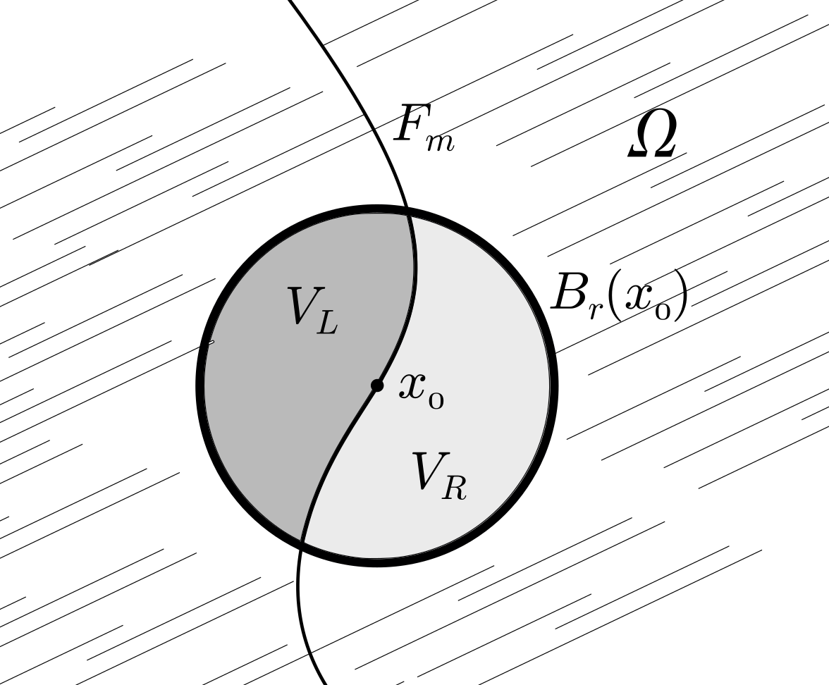
Figure 4: the elements of the proof of Lemma 8.1

Proof.

Let $x_{0}\in F_{m}$ and consider the ball, $B_{r}(x_{0})$, centered at $x_{0}$ and whose radius $r$ is small enough so that $F_{m}$ divides the ball into two regions $V_{R}:=B_{r}(x_{0})\cap\{x\,:\,m(x)>0\}$ and $V_{L}:=B_{r}(x_{0})\cap\{x\,:\,m(x)\equiv 0\}$ (see Figure 4). Furthermore, for all $x\in B_{r}(x_{0})$, define

$$\begin{split}{\mathsf{v}}_{R}(x):=\lim_{V_{R}\ni z\to x}Du(z)&;\quad m_{R}(x):=\lim_{V_{R}\ni z\to x}m(z);\\ \mathsf{v}_{L}(x):=\lim_{V_{L}\ni z\to x}Du(z)&;\quad m_{L}(x):=\lim_{V_{L}\ni z\to x}m(z)=0.\end{split}$$

Now, consider an arbitrary $\phi\in C^{\infty}(B_{r}(x_{0}))$. Then, we have the following

$$\begin{split}0&=-\int_{\Omega}\operatorname*{div}(mD_{p}H(x,Du))\phi\,dx\\ &=\int_{V_{L}}mD_{p}H(x,Du)\cdot D\phi\,dx+\int_{V_{R}}mD_{p}H(x,Du)\cdot D\phi\,dx.\end{split}$$

Notice that

$$\begin{split}\int_{V_{R}}mD_{p}H(x,Du)\cdot D\phi\,dx=-\int_{V_{R}}\operatorname*{div}(mD_{p}H(x,Du))\phi\,dx+\int_{F_{m}\cap B_{r}(x_{0})}\phi m_{R}D_{p}H(x,\mathsf{v}_{R})\cdot\nu\,ds.\end{split}$$ (8.1)

Also,

$$\begin{split}\int_{V_{L}}mD_{p}H(x,Du)\cdot D\phi\,dx=-\int_{V_{L}}\operatorname*{div}(mD_{p}H(x,Du))\phi\,dx.\end{split}$$ (8.2)

By summing the two equations, we obtain

$$\begin{split}0=\int_{F_{m}\cap B_{r}(x_{0})}\phi m_{R}D_{p}H(x,\mathsf{v}_{R})\cdot\nu\,ds.\end{split}$$

Since this is true to all $\phi\in C^{\infty}_{c}(B_{r}(x_{0}))$, we have that

$$\begin{split}m_{R}(x)D_{p}H(x,\mathsf{v}_{R}(x))\cdot\nu(x)=0\end{split}$$

for all $x\in B_{r}(x_{0})\cap F_{m}$ and $\nu$ is the outer normal to $F_{m}$. Thus, this holds true for all $x\in\Omega\cap F_{m}$. ∎

Remark 8.2.

The conclusion of this lemma, $m_{R}(x_{0})D_{p}H(x_{0},\mathsf{v}_{R}(x_{0}))\cdot\nu(x_{0})$, implies that $D_{p}H(x_{0},Du(x_{0}))$ is parallel to the free boundary, $F_{m}$, in case discontinuities appear, i.e. $m_{R}\neq 0$.

Appendix

Appendix A The Normal Trace and Neumann Boundary Condition

In this section, we discuss the Neumann boundary condition in the weak formulation of our problems, which we call the normal trace. This concept is tailored to handle the Neumann boundary condition when the gradient has low regularity, and we cannot use the classical trace theorem. The content of this section is an adaptation of the arguments in Tartar’s lecture on $H(\operatorname*{div};\Omega)$ (see [Tar07]).

A.1 Sobolev-Divergence space

For the rest of the section, we assume that $\Omega\subset\mathbb{R}^{d}$ is a bounded domain that satisfies the following segment condition on the boundary.

Definition A.1.

A set $\Omega\subset\mathbb{R}^{d}$ satisfies the segment condition on the boundary if there exist finite collections $(x_{0}^{i})_{i=1}^{N}\subset\partial\Omega$, $(r_{i})_{i=1}^{N}\subset(0,\infty)$, and $(y^{i})_{i=1}^{N}\subset\mathbb{R}^{d}$, such that

• the open balls $B_{r_{i}}(x_{0}^{i})$ cover $\partial\Omega$, and

• for every $x\in B_{r_{i}}(x_{0}^{i})\cap\overline{\Omega}$ and $t\in(0,1)$, one has

  $$\begin{split}B_{t}(x+ty^{i})\subset B_{2r_{i}}(x_{0}^{i})\cap\Omega.\end{split}$$

Remark A.2.

This condition holds when $\partial\Omega$ is $C^{1}$ or Lipschitz (possibly after some transformations).

In a divergence form problem, one would usually apply the divergence theorem with weak divergence, defined as follows.

Definition A.3.

The weak divergence or distributional divergence of function $u\in\left(L^{1}(\Omega)\right)^{d}$, denoted $\operatorname*{div}(u)$, is the linear operator that satisfies

$$\int_{\Omega}\operatorname*{div}(u)\phi=-\int_{\Omega}u\cdot D\phi$$ (A.1)

for every $\phi\in C_{c}^{\infty}(\Omega)$.

Remark A.4.

While for $u\in L^{1}$ the weak divergence is only a distribution, here, we work with functions whose weak divergence is a function. Thus, we use the integral notation in (A.1) rather than the duality pairing $\langle\cdot,\cdot\rangle$, to simplify the notation.

If $\phi$ is not compactly supported, the divergence theorem includes an extra boundary integral. This integral should be interpreted in the trace sense, which is rigorously defined in the Sobolev-divergence space, a space of functions that we examine next.

Definition A.5.

Let $\Omega\subset\mathbb{R}^{d}$ be an open subset. The weak-divergence (or Sobolev-divergence) space, $W^{\operatorname*{div},p}(\Omega)$, is the space of functions

$$\begin{split}W^{\operatorname*{div},p}(\Omega):=\{w\in(L^{p}(\Omega))^{d}\,:\,\operatorname*{div}(w)\in L^{p}(\Omega)\}.\end{split}$$

$W^{\operatorname*{div},p}(\Omega)$ is a normed space under the natural norm

$$\begin{split}||w||_{W^{\operatorname*{div},p}(\Omega)}:=\Big{(}||w||_{L^{p}(\Omega)}^{p}+||\operatorname*{div}(w)||_{L^{p}(\Omega)}^{p}\Big{)}^{1/p}.\end{split}$$

To handle limits and approximations in this space, we need two results.

Lemma A.6.

The space $W^{\operatorname*{div},p}(\Omega)$ is a Banach space.

Proof.

We only need to show that it is a complete space since the rest is trivial. So, let $\left(u_{n}\right)_{n\geq 1}$ be a Cauchy sequence in space $W^{\operatorname*{div},p}(\Omega)$. This means that $\left(\operatorname*{div}(u_{n})\right)_{n\geq 1}$ is a Cauchy sequence in $L^{p}(\Omega)$, and so is $\left(u_{n}\right)_{n\geq 1}$ in $\left(L^{p}(\Omega)\right)^{d}$. By the completeness of $L^{p}$ spaces, we have that $u_{m}\to u\in\left(L^{p}(\Omega)\right)^{d}$ and $\operatorname*{div}(u_{m})\to v\in L^{p}(\Omega)$.

We conclude the proof by showing that $\operatorname*{div}u=v$ (a.e). Take an arbitrary $\phi\in C^{\infty}_{c}(\Omega)$. Then,

$$\begin{split}\int_{\Omega}\operatorname*{div}(u)\phi=-\int_{\Omega}u\cdot D\phi=\lim_{n\to\infty}-\int_{\Omega}u_{n}\cdot D\phi=\lim_{n\to\infty}\int_{\Omega}\operatorname*{div}(u_{n})\phi=\int_{\Omega}v\phi.\end{split}$$

Therefore, $\operatorname*{div}(u)=v$ almost everywhere in $\Omega$. ∎

In the proof of the second result, we employ a slightly broader set of test functions than what is typically used. Specifically, we allow for functions that do not vanish on the boundary.

Definition A.7.

The set of test functions, $\mathfrak{D}(\overline{\Omega})$, is the set of restrictions of $C_{c}(\mathbb{R}^{d})$ on $\overline{\Omega}$.

Our goal here is to define a trace operator on $W^{\operatorname*{div},p}(\Omega)$ in a way that is consistent with the usual trace definition. We start by establishing the following result.

Proposition A.8.

Let $\Omega$ be a bounded domain in $\mathbb{R}^{d}$ that satisfies the segment condition described above. Then, $\left(\mathfrak{D}(\overline{\Omega})\right)^{d}$ is dense in $W^{\operatorname*{div},p}(\Omega)$.

Proof.

1. Let $u=(u_{1},...,u_{d})$ be an element in $W^{\operatorname*{div},p}(\Omega)$. Consider one of the open balls that cover the boundary from the segment condition; call it $B_{r}({x_{0}})$, and let $y_{0}$ be the associated vector for which $B_{t}(x+ty_{0})\subset\Omega$ for $t\in(0,1)$ and $x\in\overline{\Omega}\cap B_{r}(x_{0})$.

2. For every $t\in(0,1)$ and $x\in\overline{\Omega}\cap B_{r}(x_{0})$, define $u_{t}$ and $v_{t}$ to be the translated function $u_{t}(x)=(u_{t1},...,u_{td}):=u(x+ty_{0})$ and the mollified $v_{t}:=\eta_{t}\ast u_{t}(x)$, where $\eta_{t}(x)=c_{t}\eta(x/t)$ is the usual Sobolev mollifier.

3. Notice that

   $$\begin{split}\operatorname*{div}v_{t}(x)&=\sum_{i=1}^{d}\int_{B_{r}(x_{0})}\partial_{x_{i}}\eta_{t}(x-y)u_{ti}(y)\,dy\\ &=\sum_{i=1}^{d}\int_{B_{r}(x_{0})}-\partial_{y_{i}}\eta_{t}(x-y)u_{ti}(y)\,dy\\ &=\sum_{i=1}^{d}\int_{B_{r}(x_{0})}\eta_{t}(x-y)\partial_{y_{i}}u_{ti}(y)\,dy=(\eta_{t}\ast\operatorname*{div}u_{t})(x).\end{split}$$

   Therefore,

   $$\begin{split}&\int_{B_{r}(x_{0})}\left|\operatorname*{div}v_{t}-\operatorname*{div}u_{t}\right|^{p}\,dx=\int_{B_{r}(x_{0})}\left|\left(\eta_{t}\ast\operatorname*{div}u_{t}\right)(x)-\operatorname*{div}u_{t}(x)\right|^{p}\,dx\\ &=\int_{B_{r}(x_{0})}\left|\int_{B_{t}(0)}\frac{1}{t^{d}}\eta(z/t)(\operatorname*{div}u_{t}(x-z)-\operatorname*{div}u_{t}(x))\,dz\right|^{p}\,dx\\ &\leq C_{d}\int_{B_{r}(x_{0})}\left|\fint_{B_{t}(0)}(\operatorname*{div}u_{t}(x-z)-\operatorname*{div}u_{t}(x))\,dz\right|^{p}\,dx.\end{split}$$

   Now, we observe that

   $$\begin{split}&\int_{B_{r}(x_{0})}\left|\fint_{B_{t}(0)}(\operatorname*{div}u_{t}(x-z)-\operatorname*{div}u(x))\,dz\right|^{p}\,dx\\ &=\int_{B_{r}(x_{0})}\left|\fint_{B_{t}(0)}(\operatorname*{div}u(x+ty_{0}-z)-\operatorname*{div}u(x))\,dz\right|^{p}\,dx\\ &=\int_{B_{r}(x_{0})}\left|\fint_{B_{t}(-ty_{0})}(\operatorname*{div}u(x-z)-\operatorname*{div}u(x))\,dz\right|^{p}\,dx\end{split}$$ (A.2)

   By Corollary 5.6.3 in [Bog07] (a variant of Lebesgue’s differentiation theorem), the last line in (LABEL:eq:obs1) converges to 0 as $t\to 0$. (We remark that $B_{t}(-ty_{0})\subset B_{t+t\left|y_{0}\right|}(0)$ and that $\left|B_{t}(-ty_{0})\right|=\left(1+\left|y_{0}\right|\right)^{-d}\left|B_{t+t\left|y_{0}\right|}(0)\right|$).

∎

A.2 A lifting operator on the trace space of $W^{1,q}$

The Neuman boundary condition is often connected to integration by parts (i.e., the divergence theorem) in the following sense.

$$\begin{split}\int_{\Omega}v\,\operatorname*{div}\Phi\,\,dx=-\int_{\Omega}\Phi\cdot Dv\,\,dx+\int_{\partial\Omega}v\,\Phi\cdot\nu\,\,ds.\end{split}$$ (A.3)

The weak divergence, defined by (A.1), is, therefore, extended according to equation (A.3) to include how it acts on non-compactly supported functions. Moreover, we want to establish the boundedness of the Neuman trace $\Phi\cdot\nu$, as an element of the dual of a vector space (particularly, the dual of $W^{1-\frac{1}{q},q}(\partial\Omega)$). The desire, here, is to use equation (A.3) on functions that are (initially) defined on the boundary of $\Omega$ only. This is why we need a reasonable lifting operator that extends functions in $W^{1-\frac{1}{q},q}(\partial\Omega)$ to functions defined in the interior of $\Omega$. Such a lifting operator exists and has the correct regularity for our needs. Indeed, the following Proposition is proven in [DiB16] (Proposition 17.1c).

Proposition A.9.

Given a function $v\in W^{1-\frac{1}{q},q}(\mathbb{R}^{d-1})$, there exists an extension $\tilde{v}\in W^{1,q}(\mathbb{R}^{d}_{+})$ such that the trace of $\tilde{v}$ on the hyperplane $x_{d}=0$ is $v$. Moreover,

$$\begin{split}\left|\left|\tilde{v}(\cdot,x_{d})\right|\right|_{q,\mathbb{R}^{d-1}}&\leq\left|\left|v\right|\right|_{q,\mathbb{R}^{d-1}}\quad\quad\text{ for all }x_{d}\in(0,+\infty)\quad\text{ and}\\ \left|\left|D\tilde{v}\right|\right|_{q,\mathbb{R}^{d}_{+}}&\leq C\left|\left|v\right|\right|_{1-\frac{1}{q},q,\mathbb{R}^{d-1}}.\end{split}$$

with $C$ depending only on $q$ and $d$.

This proposition establishes the existence of a lifting operator only for the boundary of the Euclidean half-space. However, by changing variables and flattening the boundary, we can extend this Proposition to apply to a more general $C^{1}$–domain.

Theorem A.10.

Let $\Omega$ be a bounded, open, connected, $C^{1}$–domain. There exists a lifting operator $l_{0}:W^{1-\frac{1}{q},q}(\partial\Omega)\to W^{1,q}(\Omega)$ such that

$$\begin{split}\left\lVert l_{0}v\right\rVert_{W^{1,q}(\Omega)}\leq C\left\lVert v\right\rVert_{W^{1-\frac{1}{q},q}(\partial\Omega)}\end{split}$$

for every $v\in C^{\infty}(\partial\Omega)$. The constant $C$ depends only on $\Omega$ and $q$.

Proof.

By the assumptions, there is a collection of open (hyper-)cubes, $\{S_{j}\}_{j=1}^{N}$ , that covers $\partial\Omega$, such that, by rotation and rescaling, $\partial\Omega\cap S_{j}$ is the graph of a $C^{1}$ function on $[0,1]^{d-1}$. That means that, for each $j$, there is a $C^{1}$-bijection, $\Psi_{j}$, that maps $[0,1]^{d}$ to $\overline{S_{j}\cap\Omega}$ and, in a sense, flattens $\overline{\partial\Omega\cap S_{j}}$ onto $[0,1]^{d-1}$.

Now, suppose that we are given a function $v\in W^{1-\frac{1}{q},q}(\partial\Omega)$. Then the map $\overline{v}_{j}:[0,1]^{d-1}\to\mathbb{R}$ defined by $\overline{v}_{j}=v\circ\Psi_{j}$ belongs to $W^{1-\frac{1}{q},q}([0,1]^{d-1})$, which is a subsequence of the boundedness of the Jacobian of $\Psi_{j}^{-1}$ on the compact set $[0,1]^{d-1}$. The function $\overline{v}_{j}$ can be extended by a continuous extension operator from the $d-1$–dimensional cube to the entire space (see Zhou [Zho15], Theorem 1.1). Thus, we can assume that $\overline{v}_{j}\in W^{1-\frac{1}{q},q}(\mathbb{R}^{d-1})$. Whence, we can apply Proposition A.9 above, and lift $\overline{v}_{j}\in W^{1-\frac{1}{q},q}(\mathbb{R}^{d-1})$ up to $\tilde{v}_{j}\in W^{1,q}(\mathbb{R}^{d}_{+})$.

Finally, let $\{\xi_{j}\}_{j=1}^{N}$ be a smooth partition of unity subordinate to $\{S_{j}\}_{j=1}^{N}$. Then, we can define the lifting operator, $l_{0}:W^{1-\frac{1}{q},q}(\partial\Omega)\to W^{1,q}(\Omega)$, by $l_{0}v(x):=\sum_{j=1}^{N}\xi_{j}(x)\tilde{v}_{j}\circ\Psi_{j}^{-1}(x)$.

∎

A.3 The Normal Trace

Let $\gamma_{0}$ be the (usual) trace operator on the space $W^{1,q}(\Omega)$. We observe that, given a smooth $\mathbb{R}^{d}$–valued function $\Phi\in\left(\mathfrak{D}(\overline{\Omega})\right)^{d}$ and another function $v\in W^{1,q}(\Omega)$, we have

$$\begin{split}\int_{\Omega}\left[\Phi\cdot Dv+v\,\operatorname*{div}\Phi\right]\,\,dx=\int_{\partial\Omega}\Phi\cdot\nu\gamma_{0}v\,\,ds,\end{split}$$ (A.4)

where $\nu$ is the normal to $\partial\Omega$. We want to extend this identity to $\Phi\in W^{\operatorname*{div},p}(\Omega)$. For this, we need a trace operator, which is constructed in the next theorem.

Theorem A.11.

Let $\Omega$ be an open, bounded, $C^{1}$–domain. Then, there is a bounded linear operator

$$\begin{split}\gamma_{1}:W^{\operatorname*{div},p}(\Omega)\to W^{-(1-\frac{1}{p^{\prime}}),p^{\prime}}(\partial\Omega)\end{split}$$

such that the following are satisfied.

1. The operator $\gamma_{1}$ is consistent with the evaluation point-wise on the boundary for smooth function; that is, $\gamma_{1}(u)=u|_{\partial\Omega}\cdot\nu$ for all $u\in W^{\operatorname*{div},p}(\Omega)\cap\left(\mathfrak{D}(\overline{\Omega})\right)^{d}$.

2. For each $u\in W^{\operatorname*{div},p}(\Omega)$, $\gamma_{1}(u)$ is bounded as a linear operator on $W^{1-\frac{1}{p^{\prime}},p^{\prime}}(\partial\Omega)$; particularly,

   $$\left|\langle\gamma_{1}(u),v\rangle\right|\leq C(u)\left\lVert v\right\rVert_{1-\frac{1}{p^{\prime}},p^{\prime}}$$ (A.5)

Proof.

This is done using the previous density result (Proposition A.8) and the lifting operator.

1. We prove boundedness for the smooth functions first. Consider an arbitrary vector-valued function $u\in\left(\mathfrak{D}(\overline{\Omega})\right)^{d}$. Define $\gamma_{1}(u)=u|_{\partial\Omega}\cdot\nu$. We notice that, as an element of $W^{-(1-\frac{1}{p^{\prime}}),p^{\prime}}(\partial\Omega)$, the Neumann trace $\gamma_{1}(u)$ satisfies

   $$\begin{split}\left|\langle\gamma_{1}(u),v\rangle\right|=\left|\int_{\partial\Omega}\gamma_{1}(u)\,v\,ds\right|=\left|\int_{\Omega}Dl_{0}v\cdot u+l_{0}v\,\operatorname*{div}u\right|&\leq\left\lVert u\right\rVert_{W^{\operatorname*{div},p}(\Omega)}\left\lVert l_{0}v\right\rVert_{W^{1,p^{\prime}}(\Omega)}\\ &\leq C\left\lVert u\right\rVert_{W^{\operatorname*{div},p}(\Omega)}\left\lVert v\right\rVert_{1-\frac{1}{p^{\prime}},p^{\prime},\partial\Omega}.\end{split}$$ (A.6)

   Hence, $\gamma_{1}$ is a bounded operator.

   Hence, $\gamma_{1}\in W^{-(1-\frac{1}{p^{\prime}}),p^{\prime}}(\partial\Omega)$ is a bounded linear operator.

2. Because $\left(\mathfrak{D}(\overline{\Omega})\right)^{d}$ is dense in $W^{\operatorname*{div},p}(\Omega)$, we can define $\gamma_{1}(u)$ for an arbitrary $u\in W^{\operatorname*{div},p}(\Omega)$ as the limit

   $$\langle\gamma_{1}(u),v\rangle=\lim\limits_{n}\langle\gamma_{1}(u_{n}),v\rangle$$

   for any sequence $\{u_{n}\}\subset\left(\mathfrak{D}(\overline{\Omega})\right)^{d}\cap W^{\operatorname*{div},p}(\Omega)$ and every $v\in W^{-(1-\frac{1}{p^{\prime}}),p^{\prime}}(\partial\Omega)$.

∎

Remark A.12.

It is worth noting that the convergence of the sequence $\langle\gamma_{1}(u_{n}),v\rangle$ is mere convergence of scalars (reals). It doesn’t pose any technical issues as long as we can prove it is a Cauchy sequence, which comes directly from the inequality (A.6).

References

- [Ber18] Charles Bertucci. Optimal stopping in mean field games, an obstacle problem approach. Journal de Mathématiques Pures et Appliquées, 120:165–194, 2018.
- [Bog07] Vladimir Bogachev. Measure theory. Vol. I, II. Springer-Verlag, Berlin, 2007.
- [CG15] Pierre Cardaliaguet and P. Jameson Graber. Mean field games systems of first order. ESAIM: COCV, 21(3):690–722, 2015.
- [Cir15] Marco Cirant. Multi-population mean field games systems with neumann boundary conditions. Journal de Mathématiques Pures et Appliquées, 103(5):1294–1315, 2015.
- [DiB16] Emmanuele DiBenedetto. Real Analysis. Birkhäuser, 2016.
- [FGT19] Rita Ferreira, Diogo Gomes, and Teruo Tada. Existence of weak solutions to first-order stationary mean-field games with Dirichlet conditions. Proc. Amer. Math. Soc., pages 4713–4731, 2019.
- [GPV16] Diogo Gomes, Edgard Pimentel, and Vardan Voskanyan. Regularity theory for mean-field game systems. Springer Nature, 2016.
- [HCM07] Minyi Huang, Peter Caines, and Roland Malhamé. Large-population cost-coupled LQG problems with non-uniform agents: individual-mass behavior and decentralized -Nash equilibria. Automatic Control, (3):1560–1571, 2007.
- [HMC06] Minyi Huang, Roland Malhamé, and Peter Caines. Large population stochastic dynamic games: closed- loop McKean-Vlasov systems and the Nash certainty equivalence principle. Communcations in Information and Systems, (3):221–251, 2006.
- [LL06a] Jean-Michel Lasry and Pierre-Louis Lions. Jeux à champ moyen. I – le cas stationnaire. Comptes Rendus Mathematique, 343(9):619–625, 2006.
- [LL06b] Jean-Michel Lasry and Pierre-Louis Lions. Jeux à champ moyen. II – horizon fini et contrôle. Comptes Rendus Mathematique, 343(9):679–684, 2006.
- [LL07] Jean-Michel Lasry and Pierre-Louis Lions. Mean field games. Japanese Journal of Mathematics, (1):229–260, 2007.
- [MS18] Alpár Mészáros and Francisco Silva. On the variational formulation of some stationary second-order mean field games systems. SIAM Journal on Mathematical Analysis, 50(1):1255–1277, 2018.
- [Tar07] Luc Tartar. An introduction to Sobolev spaces and interpolation spaces, volume 3 of Lecture Notes of the Unione Matematica Italiana. Springer, Berlin; UMI, Bologna, 2007.
- [Zho15] Yuan Zhou. Fractional Sobolev extension and imbedding. Trans. Amer. Math. Soc., 367(2):959–979, 2015.