Learning Directed Graphical Models with Optimal Transport

Abstract

Estimating the parameters of a probabilistic directed graphical model from incomplete data is a long-standing challenge. This is because, in the presence of latent variables, both the likelihood function and posterior distribution are intractable without further assumptions about structural dependencies or model classes. While existing learning methods are fundamentally based on likelihood maximization, here we offer a new view of the parameter learning problem through the lens of optimal transport. This perspective licenses a general framework that operates on any directed graphs without making unrealistic assumptions on the posterior over the latent variables or resorting to variational approximations. We develop a theoretical framework and support it with extensive empirical evidence demonstrating the versatility and robustness of our approach. Across experiments, we show that not only can our method effectively recover the ground-truth parameters but it also performs comparably or better on downstream applications.

1 Introduction

Learning probabilistic directed graphical models (DGMs, also known as Bayesian networks) with latent variables is an ongoing challenge in machine learning and statistics. This paper focuses on parameter learning, i.e., estimating the parameters of a DGM given its known structure. Learning DGMs has a long history, dating back to classical indirect likelihood-maximization approaches such as expectation maximization (EM, Dempster et al., 1977). Despite all its success stories, EM is well-known to suffer from local optima issues. More importantly, EM becomes inapplicable when the posterior distribution is intractable, which arises fairly often in practice. Furthermore, EM is originally a batch algorithm, thereby converging slowly on large datasets (Liang & Klein, 2009). Subsequently, researchers have explored combining EM with approximate inference along with other strategies increasing efficiency (Wei & Tanner, 1990; Neal & Hinton, 1998; Delyon et al., 1999; Beal & Ghahramani, 2006; Cappé & Moulines, 2009; Liang & Klein, 2009; Neath et al., 2013). A large family of approximation algorithms based on variational inference (VI, Jordan et al., 1999; Hoffman et al., 2013) have demonstrated tremendous potential, where the evidence lower bound (ELBO) is not only used for posterior approximation but also for point estimation of the model parameters. Such an approach has proved surprisingly effective and robust to overfitting, especially when having a small number of parameters. VI has recently taken a leap forward by embracing amortized inference (Amos, 2022), which performs black-box optimization in a considerably more efficient way.

Prior to estimating the parameters, both EM and VI consist of an inference step which ultimately requires carrying out expectations of the commonly intractable posterior over the latent variables. In order to address this challenge, a large spectrum of methods have been proposed in the literature and we refer the reader to Ambrogioni et al. (2021) for an excellent discussion of these approaches. Here we characterize them between two extremes. At one extreme, restrictive assumptions about the structure (e.g., as in mean-field approximations) or the model class (e.g., using conjugate exponential families) must be made to simplify the task. At the other extreme, when no assumptions are made, most existing black-box methods exploit very little information about the structure of the known probabilistic model (e.g., in black-box and stochastic VI (Ranganath et al., 2014; Hoffman et al., 2013), hierarchical approaches (Ranganath et al., 2016) or normalizing flows (Papamakarios et al., 2021)). Section 2 summarizes the progression of VI research towards this extreme. Since the ultimate goal of VI is posterior inference, parameter estimation has been treated as a by-product of the optimization process where the model parameters are cast as global latent variables. As the complexity of the graph increases, parameter estimation in VI becomes computationally challenging.

A natural question arises as to whether one can learn the parameters of any DGMs with hidden nodes without explicitly solving inference nor assuming any structural independencies. In this work, we revisit the classic problem of learning graphical models from the viewpoint of optimal transport (OT, Villani et al., 2009), which permits a scalable and general framework that addresses the above criterion.

OT as an alternative to MLE.

Estimating the model parameters is essentially about learning a probability density from empirical data. EM and VI are fundamentally based on maximum likelihood estimation (MLE), which amounts to, asymptotically, minimizing the KL (Kullback-Leibler) divergence the true data and model distribution. We here propose to find a point estimate that minimizes the Wasserstein (WS) distance (Kantorovich, 1960) between these two distributions. The motivations of using WS distance to this problem are three-fold.

First, the measurability and consistency of the minimum Wasserstein estimators have been rigorously studied in prior research, notably in Bassetti et al. (2006); Bernton et al. (2019). Second, WS distance is a metric, thus serving as a more sensible measure of distance between two distributions, especially those that are supported on low dimensional manifolds with negligible intersection of support, where standard metrics such as the KL or JS (Jensen-Shannon) divergences are either infinite or undefined (Peyré et al., 2017; Ambrogioni et al., 2018). This property has motivated the recent surge in generative models, namely Wasserstein GANs (WGAN, Adler & Lunz, 2018; Arjovsky et al., 2017) and Wasserstein Auto-encoders (WAE, Tolstikhin et al., 2017). Underlying WAE is basically a two-node graphical model with one observed node (i.e., the data) and one latent node (i.e., often a Gaussian prior). There has also been application of OT for learning Gaussian mixture models (GMM), underlying which is also a two-node graphical model where the latent variable (i.e., the mixture weight) is categorical. Mena et al. (2020) proposes an algorithm named Sinkhorn EM using entropic OT loss which yields faster convergence rate than vanilla EM. Kolouri et al. (2018) studies the extension of the Wasserstein mean problem (Ho et al., 2017) to learn a GMM, showing that the Wasserstein energy landscape is smoother and less sensitive to the initial point than that of the negative log likelihood.

Finally, we substantiate the motivation of using OT for graphical learning with an additional experiment of learning GMM under mis-specifications. The task is to estimate the means of a mixture of two bi-variate Gaussian distributions with unit variance i.e., $\sigma_{1}=\sigma_{2}=\mathbf{I}$. The means of one Gaussian are $\mu_{11},\mu_{12}\sim{\mathcal{U}}(0,2)$ and the means of the other are $\mu_{21},\mu_{22}\sim{\mathcal{U}}(0,2)$. The mixture weight is $\pi\sim{\mathcal{U}}(0.50,0.70)$. Figure 1 illustrates the mean absolute errors when (1) the variances are mis-specified at $\varepsilon_{\sigma}\mathbf{I}$ where $\varepsilon_{\sigma}\sim{\mathcal{U}}(1,2)$; (2) the weights are mis-specified at $\varepsilon_{\pi}\sim{\mathcal{U}}(0,1)$; (3) both are mis-specified. We compare EM with our proposed method that estimates the means by the minimum Wasserstein estimators. The figures show that while EM plateaus early on, our method continues to converge over training. This reaffirms that minimum Wasserstein estimators tend to be more reliable and robust under mis-specifications (Bernton et al., 2019). Despite the above desirable properties of the WS distance, the application of OT to learning a general graphical model remains unexplored. Our work is proposed to fill in this gap.

Contributions.

In this work, we introduce OTP-DAG, an Optimal Transport framework for Parameter Learning in Directed Acyclic Graphical models. OTP-DAG is a flexible framework applicable to any type of variables and graphical structure. Our theoretical development renders a tractable formulation of the Wasserstein objective for models with latent variables, which is established as a generalization for the WAE model. We further provide empirical evidence demonstrating the versatility of our method on various graphical structures, where OTP-DAG is shown to successfully recover the ground-truth parameters and achieve comparable or better performance than competing methods across a range of downstream applications.

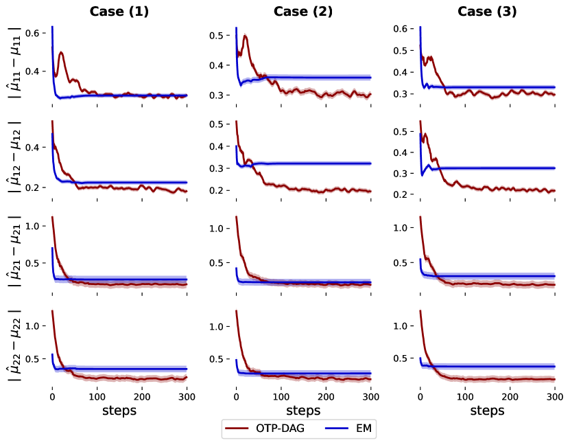
Figure 1: Visualization of mean absolute errors of the inferred means $\hat{\mu}$ and the true values $\mu$ for $300$ steps, averaged over $100$ simulations. $\mu_{ki}$ indicates the mean of the component $k$ at dimension $i$. The red line represents our method OTP-DAG. The blue line represents EM. Three mis-specified cases are studied: Case (1) mis-specified variances, Case (2) mis-specified weights and Case (3) mis-specified both variances and weights.

2 Related work

As part of parameter learning, both EM and VI entail an inference sub-process for posterior estimation. If the posteriors cannot be computed exactly, approximate inference is the go-to solution. In this section, we focus on variational algorithms and their computational challenges. Along this line, research efforts have concentrated on ensuring tractability of the ELBO via the mean-field assumption (Bishop & Nasrabadi, 2006) and its relaxation known as structured mean field (Saul & Jordan, 1995). Scalability has been one of the main challenges facing the early VI formulations since optimization is done per-sample basis. This has triggered the development of stochastic variational inference (SVI, Hoffman et al., 2013; Hoffman & Blei, 2015; Foti et al., 2014; Johnson & Willsky, 2014; Anandkumar et al., 2012, 2014) which applies stochastic optimization to solve VI objectives. Another line of work is collapsed VI that explicitly integrates out certain model parameters or latent variables in an analytic manner (Hensman et al., 2012; King & Lawrence, 2006; Teh et al., 2006; Lázaro-Gredilla et al., 2012). Without a closed form, one could resort to Markov chain Monte Carlo (Gelfand & Smith, 1990; Gilks et al., 1995; Hammersley, 2013), which however tends to be slow. More accurate variational posteriors also exist, namely, through hierarchical variational models (Ranganath et al., 2016), implicit posteriors (Titsias & Ruiz, 2019; Yin & Zhou, 2018; Molchanov et al., 2019; Titsias & Ruiz, 2019), normalizing flows (Kingma et al., 2016), or copula distribution (Tran et al., 2015). To avoid computing the ELBO analytically, one can obtain an unbiased gradient estimator using re-parameterization tricks (Ranganath et al., 2014; Xu et al., 2019). Extensions of VI to other divergence measures such as $\alpha-$divergence or $f-$divergence, also exist in Li & Turner (2016); Hernandez-Lobato et al. (2016); Wan et al. (2020). A thorough review the above approaches can be found in (Ambrogioni et al., 2021, §6).

3 Preliminaries

We first introduce the notations and basic concepts used throughout the paper. We reserve bold capital letters (i.e., ${\mathbf{G}}$) for notations related to graphs. We use calligraphic letters (i.e. ${\mathcal{X}}$) for spaces, italic capital letters (i.e. $X$) for random variables, and lower case letters (i.e. $x$) for values.

A directed graph ${\mathbf{G}}=({\mathbf{V}},{\mathbf{E}})$ consists of a set of nodes ${\mathbf{V}}$ and an edge set ${\mathbf{E}}\subseteq{\mathbf{V}}^{2}$ of ordered pairs of nodes with $(v,v)\notin{\mathbf{E}}$ for any $v\in{\mathbf{V}}$ (one without self-loops). For a pair of nodes $i,j$ with $(i,j)\in{\mathbf{E}}$, there is an arrow pointing from $i$ to $j$ and we write $i\rightarrow j$. Two nodes $i$ and $j$ are adjacent if either $(i,j)\in{\mathbf{E}}$ or $(j,i)\in{\mathbf{E}}$. If there is an arrow from $i$ to $j$ then $i$ is a parent of $j$ and $j$ is a child of $i$. A Bayesian network structure ${\mathbf{G}}=({\mathbf{V}},{\mathbf{E}})$ is a directed acyclic graph (DAG), in which the nodes represent random variables $X=[X_{i}]^{n}_{i=1}$ with index set ${\mathbf{V}}:=\{1,...,n\}$. Let $\mathrm{PA}_{X_{i}}$ denote the set of variables associated with parents of node $i$ in ${\mathbf{G}}$. In this work, we tackle the classic yet important problem of learning the parameters of a directed graph from partially observed data. Let ${\mathbf{O}}\subseteq{\mathbf{V}}$ and $X_{\mathbf{O}}=[X_{i}]_{i\in{\mathbf{O}}}$ be the set of observed nodes and ${\mathbf{H}}:={\mathbf{V}}\backslash{\mathbf{O}}$ be the set of hidden nodes. Let $P_{\theta}$ and $P_{d}$ respectively denote the distribution induced by the graphical model and the empirical one induced by the complete (yet unknown) data. Given a fixed graphical structure ${\mathbf{G}}$ and some set of i.i.d data points, we aim to find the point estimate $\theta^{*}$ that best fits the observed data $X_{{\mathbf{O}}}$. The conventional approach is to minimize the KL divergence between the model distribution and the empirical data distribution over observed data i.e., $\textrm{KL}(P_{d}(X_{{\mathbf{O}}}),P_{\theta}(X_{{\mathbf{O}}}))$, which is equivalent to maximizing the likelihood $P_{\theta}(X_{{\mathbf{O}}})$ w.r.t $\theta$. In the presence of latent variables, the marginal likelihood, given as $P_{\theta}(X_{\mathbf{O}})=\int_{X_{{\mathbf{H}}}}P_{\theta}(X)dX_{{\mathbf{H}}}$, is generally intractable.

4 Optimal Transport for Learning Directed Graphical Models

We consider a DAG ${\mathbf{G}}({\mathbf{V}},{\mathbf{E}})$ over random variables $X=[X_{i}]^{n}_{i=1}$ that represents the data generative process of an underlying system. The system consists of $X$ as the set of endogenous variables and $U=\{U_{i}\}^{n}_{i=1}$ as the set of exogenous variables representing external factors affecting the system. Associated with every $X_{i}$ is an exogenous variable $U_{i}$ whose values are sampled from a prior distribution $P(U)$ independently from the other exogenous variables. For the purpose of theoretical development, our framework operates on an extended graph consisting of both endogenous and exogenous nodes (See Figure 2). In the graph ${\mathbf{G}}$, $U_{i}$ is represented by a node with no ancestors that has an outgoing arrow towards itself. Every distribution $P_{\theta_{i}}\big{(}X_{i}|\mathrm{PA}_{X_{i}}\big{)}$ can be reparameterized into a deterministic assignment

$$X_{i}:=\psi_{i}\big{(}\mathrm{PA}_{X_{i}},U_{i}\big{)},\ \text{for }i=1,...,n.$$

The ultimate goal is to estimate $\theta=\{\theta_{i}\}_{i=1}^{n}$ as the parameters of the set of deterministic functions $\psi=\{\psi_{i}\}_{i=1}^{n}$. We will use the notation $\psi_{\theta}$ to emphasize this connection from now on. Given the empirical data distribution $P_{d}(X_{{\mathbf{O}}})$ and the model distribution $P_{\theta}(X_{{\mathbf{O}}})$ over the observed set ${\mathbf{O}}$, the optimal transport (OT) goal is to find the parameter set $\theta$ that minimizes the cost of transport between these two distributions. The Kantorovich’s formulation of the problem is given by

$$W_{c}\big{(}P_{d};P_{\theta}\big{)}:=\inf_{\Gamma\sim{\mathcal{P}}(X\sim P_{d},Y\sim P_{\theta})}\mathbb{E}_{(X,Y)\sim\Gamma}\bigl{[}c(X,Y)\bigr{]},$$ (1)

where ${\mathcal{P}}(X\sim P_{d},Y\sim P_{\theta})$ is a set of all joint distributions of $\big{(}P_{d};P_{\theta}\big{)}$; $c:{\mathcal{X}}_{{\mathbf{O}}}\times{\mathcal{X}}_{{\mathbf{O}}}\mapsto{\mathcal{R}}_{+}$ is any measurable cost function over ${\mathcal{X}}_{{\mathbf{O}}}$ (i.e., the product space of the spaces of observed variables) defined as $c(X_{\mathbf{O}},Y_{\mathbf{O}}):=\sum_{i\in{\mathbf{O}}}c_{i}(X_{i},Y_{i})$ where $c_{i}$ is a measurable cost function over a space of an observed variable.

Since $P_{\theta}$ is intractable due to the latent factor, the formulation in Eq. (1) cannot be directly optimized. We now propose our solution to this problem.

Let $P_{\theta}(\mathrm{PA}_{X_{i}},U_{i})$ denote the joint distribution of $\mathrm{PA}_{X_{i}}$ and $U_{i}$ factorized according to the graphical model. Let ${\mathcal{U}}_{i}$ denote the space over random variable $U_{i}$. The key ingredient of our theoretical development is local backward mapping. For every observed node $i\in{\mathbf{O}}$, we define a stochastic “backward” map $\phi_{i}:{\mathcal{X}}_{i}\mapsto\Pi_{k\in\mathrm{PA}_{X_{i}}}\ {\mathcal{X}}_{k}\times{\mathcal{U}}_{i}$ such that $\phi_{i}\in\mathfrak{C}(X_{i})$ where $\mathfrak{C}(X_{i})$ is the constraint set given as

$$\mathfrak{C}(X_{i}):=\bigl{\{}\phi_{i}:\phi_{i}\#P_{d}(X_{i})=P_{\theta}(\mathrm{PA}_{X_{i}},U_{i})\bigr{\}};$$

that is, every backward $\phi_{i}\#$ defines a push forward operator such that the samples from $\phi_{i}(X_{i})$ follow the marginal distribution $P_{\theta}(\mathrm{PA}_{X_{i}},U_{i})$. Let $P_{\phi_{i}}(\mathrm{PA}_{X_{i}},U_{i})=\mathbb{E}_{X_{i}}\left[\phi_{i}(\mathrm{PA}_{X_{i}},U_{i}|X_{i})\right]$ denote the marginal distribution induced by every $\phi_{i}$.

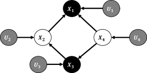
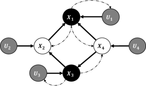
Figure 2: (Left) A DAG represents a system of $4$ endogenous variables where $X_{1},X_{3}$ are observed (black-shaded) and $X_{2},X_{4}$ are hidden variables (non-shaded). (Middle) The extended DAG includes an additional set of independent exogenous variables $U_{1},U_{2},U_{3},U_{4}$ (grey-shaded) acting on each endogenous variable. $U_{1},U_{2},U_{3},U_{4}\sim P(U)$ where $P(U)$ is a prior product distribution. (Right) Visualization of our backward-forward algorithm, where the dashed arcs represent the backward maps involved in optimization.

We will show that the optimization problem (OP) in (1) can be reduced to minimizing the reconstruction error between the observed data and the data generated from $P_{\theta}$. To understand how the reconstruction works, let us examine the right illustration in Figure 2. With a slight abuse of notations, for every $X_{i}$, we extend its parent set $\mathrm{PA}_{X_{i}}$ to include an exogenous variable and possibly some other endogenous variables. Given $X_{1}$ and $X_{3}$ as observed nodes, we first sample $X_{1}\sim P_{d}(X_{1}),X_{3}\sim P_{d}(X_{3})$ and then construct backward maps $\phi_{1},\phi_{3}$. The next step is to sample $\textrm{PA}_{X_{1}}\sim\phi_{1}(\textrm{PA}_{X_{1}}|X_{1})$ and $\textrm{PA}_{X_{3}}\sim\phi_{3}(\textrm{PA}_{X_{3}}|X_{3})$, where $\textrm{PA}_{X_{1}}=\{X_{2},X_{4},U_{1}\}$ and $\textrm{PA}_{X_{3}}=\{X_{4},U_{3}\}$, which are plugged back to the model $\psi_{\theta}$ to obtain the reconstructions $\widetilde{X_{1}}=\psi_{\theta_{1}}(\textrm{PA}_{X_{1}})$ and $\widetilde{X_{3}}=\psi_{\theta_{3}}(\textrm{PA}_{X_{3}})$. We wish to learn $\theta$ such that $X_{1}$ and $X_{3}$ are reconstructed correctly. For a general graphical model, this optimization objective is formalized as

Theorem 4.1.

For every $\phi_{i}$ as defined above and fixed $\psi_{\theta}$,

$$W_{c}\big{(}P_{d}(X_{\mathbf{O}});P_{\theta}(X_{\mathbf{O}})\big{)}=$$

$$\inf_{\bigl{[}\phi_{i}\in\mathfrak{C}(X_{i})\bigr{]}_{i\in{\mathbf{O}}}}\mathbb{E}_{X_{\mathbf{O}}\sim P_{d},\mathrm{PA}_{X_{\mathbf{O}}}\sim P_{\phi}}\bigl{[}c\bigl{(}X_{\mathbf{O}},\psi_{\theta}(\mathrm{PA}_{X_{\mathbf{O}}})\bigr{)}\bigr{]},$$ (2)

where $\mathrm{PA}_{X_{\mathbf{O}}}:=\big{[}[X_{ij}]_{j\in\mathrm{PA}_{X_{i}}}\big{]}_{i\in{\mathbf{O}}}$.

Proof.

See Appendix A.

Our OT problem seeks to find the optimal set of deterministic “forward” maps $\psi_{\theta}$ and stochastic “backward” maps $\big{\{}\phi_{i}\in\mathfrak{C}(X_{i})\big{\}}_{i\in{\mathbf{O}}}$ that minimize the cost of transporting the mass from $P_{d}$ to $P_{\theta}$ over ${\mathbf{O}}$. While Theorem 4.1 set ups a tractable form for our optimization solution, note that our OP is constrained, where every backward function $\phi_{i}$ must satisfy its push-forward condition defined by $\mathfrak{C}$. In the above example, the backward maps $\phi_{i}$ and $\phi_{3}$ must be constructed such that $\phi_{1}\#P_{d}(X_{1})=P_{\theta}(X_{2},X_{4},U_{1})$ and $\phi_{3}\#P_{d}(X_{3})=P_{\theta}(X_{4},U_{3})$. We propose to relax the constraints by adding a penalty to the above objective.

The final optimization objective is therefore given as

$$\inf_{\theta}\ \inf_{\phi}\mathbb{E}_{X_{\mathbf{O}}\sim P_{d},\mathrm{PA}_{X_{\mathbf{O}}}\sim\phi(X_{\mathbf{O}})}\bigl{[}c\bigl{(}X_{\mathbf{O}},\psi_{\theta}(\mathrm{PA}_{X_{\mathbf{O}}})\bigr{)}\bigr{]}$$

$$\quad\quad\quad\quad+\eta\ D\big{(}P_{\phi},P_{\theta}\big{)}$$ (3)

where $D$ is any arbitrary divergence measure and $\eta>0$ is a trade-off hyper-parameter. $D\big{(}P_{\phi},P_{\theta}\big{)}$ is a short-hand for divergence between all pairs of backward and forward distributions.

Remark.

Eq. (4) renders an optimization-based approach in which we leverage reparameterization and amortized inference (Amos, 2022) for solving it efficiently via stochastic gradient descent. This theoretical result provides our OTP-DAG with two interesting properties: (1) all model parameters are optimized simultaneously within a single framework whether the variables are continuous or discrete, and (2) the computational process can be automated without the need for analytic lower bounds (as in EM and traditional VI), specific graphical structures (as in mean-field VI), or priors over variational distributions on latent variables (as in hierarchical VI). The flexibility our method exhibits is akin to auto-encoding models, and OTP-DAG in fact serves as an extension of WAE for learning general directed graphical models. Our formulation thus inherits a desirable characteristic from that of WAE, which specifically helps mitigate the posterior collapse issue notoriously occurring to VAE. Appendix B explains this behavior in more detail. Particularly, in the next section, we will empirically show that OTP-DAG effectively alleviates the codebook collapse issue in discrete representation learning. Algorithm 1 provides the pseudo-code for OTP-DAG learning procedure.

Algorithm 1 OTP-DAG Algorithm

  Input: Directed graph ${\mathbf{G}}$ with observed nodes ${\mathbf{O}}$, noise distribution $P(U)$, regularization coefficient $\eta$, reconstruction cost function $c$, and divergence measure $D$.

  Output: Point estimate $\theta$.

  Initialize a set of deterministic assignments $\psi_{\theta}=\{\psi_{\theta_{i}}\}_{i\in{\mathbf{O}}}$ where $X_{i}:=\psi_{\theta_{i}}(\textrm{PA}_{X_{i}},U_{i})$ and $U_{i}\sim P(U)$;

  Initialize the stochastic maps $\phi=\{\phi_{i}(X_{i})\}_{i\in{\mathbf{O}}}$;

  while $(\phi,\theta)$ not converged do

       for $i\in{\mathbf{O}}$,

• Sample batch $X^{B}_{i}=\{x^{1}_{i},...,x^{B}_{i}\}$;

• Sample $\widetilde{\textrm{PA}}_{X^{B}_{i}}$ from $\phi_{i}(X^{B}_{i})$;

• Sampling $U_{i}$ from the prior $P(U)$;

• Evaluate $\widetilde{X}^{B}_{i}=\psi_{\theta_{i}}(\widetilde{\textrm{PA}}_{X^{B}_{i}},U_{i})$.

  Update $\phi$ and $\theta$ iteratively by descending

$$\frac{1}{B}\sum_{b=1}^{B}\sum_{i\in{\mathbf{O}}}c\big{(}x_{i}^{b},\widetilde{x}_{i}^{b}\big{)}+\eta\ D\big{[}P_{\phi_{i}}(\textrm{PA}_{X_{i}^{B}}),P_{\theta}(\textrm{PA}_{X_{i}^{B}})\big{]}$$

  end while

5 Applications

In this section, we illustrate the practical application of the OTP-DAG algorithm. We consider various directed probabilistic models with different types of latent variables (continuous and discrete) and for different types of data (texts, images, and time series). In all tables, we report the average results over $5$ random initializations and the best/second-best ones are bold/underlined. $\uparrow$, $\downarrow$ indicate higher/lower performance is better, respectively.

Baselines.

We compare OTP-DAG with two groups of parameter learning methods towards the two extremes: (1) EM and SVI where analytic derivation is required; (2) variational auto-encoding frameworks where black-box optimization is permissible. We leave the discussion of the formulation and technicalities in Appendix C.

Experimental setup.

We begin with (1) Latent Dirichlet Allocation (Blei et al., 2003), a simple and popular task of topic modeling where traditional methods like EM or SVI can solve. We then consider learning (2) Hidden Markov Model (HMM), which remains fairly challenging, with known optimization/inference algorithms (e.g., Baum-Welch algorithm) often too computationally costly to be used in practice. We conclude with a more challenging setting: (3) Discrete Representation Learning (Discrete RepL) that cannot simply be solved by EM or MAP (maximum a posteriori). It in fact invokes deep generative modeling via a pioneering development called Vector Quantization Variational Auto-Encoder (VQ-VAE, Van Den Oord et al., 2017). We attempt to apply OTP-DAG for learning discrete representations by grounding it into a parameter learning problem. Figure 3 illustrates the empirical DAG structures of $3$ applications. Unlike the standard visualization where the parameters are considered hidden nodes, our graph separates model parameters from latent variables and only illustrates random variables and their dependencies (except the special setting of Discrete RepL). We also omit the exogenous variables associated with the hidden nodes for visibility, since only those acting on the observed nodes are relevant for computation. There is also a noticeable difference between Figures 3 and 2: the empirical version does not require learning the backward maps for the exogenous variables. It is observed across our experiments that sampling the noise from an appropriate prior distribution suffices to yield accurate estimation, which is in fact beneficial in that training time can be greatly reduced.

Takeaways.

In the following, we show that in the simulated settings where the models are well-specified, OTP-DAG performs equally well as the baseline methods, while exhibits superior efficiency over EM on such a complex graph as HMM. Furthermore, OTP-DAG is shown to achieve better performance on real-world downstream tasks, which substantiates the robustness of minimum Wasserstein estimators in practical settings. Finally, throughout the experiments, we also aim to demonstrate the versatility of OTP-DAG where our method can be harnessed for a wide range of purposes in a single learning procedure.

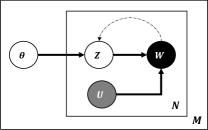
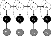
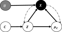
Figure 3: Empirical structures of (left) latent Dirichlet allocation model (in plate notation), (middle) standard hidden Markov model, and (right) discrete representation learning.

5.1 Latent Dirichlet Allocation

Let us consider a corpus ${\mathcal{D}}$ of $M$ independent documents where each document is a sequence of $N$ words denoted by $W=(W_{1},W_{2},\cdots,W_{N})$. Documents are represented as random mixtures over $K$ latent topics, each of which is characterized by a distribution over words. Let $V$ be the size of a vocabulary indexed by $\{1,\cdots,V\}$. Latent Dirichlet Allocation (LDA) (Blei et al., 2003) dictates the following generative process for every document in the corpus:

1. Sample $\theta\sim\textrm{Dir}(\alpha)$ with $\alpha<1$,

2. Sample $\gamma_{k}\sim\textrm{Dir}(\beta)$ where $k\in\{1,\cdots,K\}$,

3. For each of the word positions $n\in\{1,\cdots,N\}$,

   • Sample a topic $Z_{n}\sim\textrm{Multi-nominal}(\theta)$,

   • Sample a word $W_{n}\sim\textrm{Multi-nominal}(\gamma_{k})$,

where $\textrm{Dir}(.)$ is a Dirichlet distribution. $\theta$ is a $K-$dimensional vector that lies in the $(K-1)-$simplex and $\gamma_{k}$ is a $V-$dimensional vector represents the word distribution corresponding to topic $k$. In the standard model, $\alpha,\beta,K$ are hyper-parameters and $\theta,\gamma$ are learnable parameters. Throughout the experiments, the number of topics $K$ is assumed known and fixed.

Parameter Estimation.

To test whether OTP-DAG can recover the true parameters, we generate synthetic data in the setting: the word probabilities are parameterized by a $K\times V$ matrix $\gamma$ where $\gamma_{kn}:=P(W_{n}=1|Z_{n}=1)$; $\gamma$ is now a fixed quantity to be estimated. We set $\alpha=1/K$ uniformly and generate small datasets for different number of topics $K$ and sample size $N$. Following (Griffiths & Steyvers, 2004), for every topic $k$, the word distribution $\gamma_{k}$ can be represented as a square grid where each cell, corresponding to a word, is assigned an integer value of either $0$ and $1$, indicating whether a certain word is allocated to the $k^{th}$ topic or not. As a result, each topic is associated with a specific pattern. For simplicity, we represent topics using horizontal or vertical patterns (See Figure 4). According to the above generative model, we sample data w.r.t $3$ sets of configuration triplets $\{K,M,N\}$. We compare OTP-DAG with Batch EM and SVI and Prod LDA - a variational auto-encoding topic model (Srivastava & Sutton, 2017).

Table 1: Fidelity of estimates of the topic-word distribution $\gamma$ across $3$ settings. Fidelity is measured by KL divergence, Hellinger (HL) (Hellinger, 1909) and Wasserstein distance with the true $\gamma$.

Metric $\downarrow$	$K$	$M$	$N$	OTP-DAG (Ours)	Batch EM	SVI	Prod LDA
HL	10	1,000	100	2.327 $\pm$ 0.009	2.807 $\pm$ 0.189	2.712 $\pm$ 0.087	2.353 $\pm$ 0.012
KL	10	1,000	100	1.701 $\pm$ 0.005	1.634 $\pm$ 0.022	1.602 $\pm$ 0.014	1.627 $\pm$ 0.027
WS	10	1,000	100	0.027 $\pm$ 0.004	0.058 $\pm$ 0.000	0.059 $\pm$ 0.000	0.052 $\pm$ 0.001
HL	20	5,000	200	3.800 $\pm$ 0.058	4.256 $\pm$ 0.084	4.259 $\pm$ 0.096	3.700 $\pm$ 0.012
KL	20	5,000	200	2.652 $\pm$ 0.080	2.304 $\pm$ 0.004	2.305 $\pm$ 0.003	2.316 $\pm$ 0.026
WS	20	5,000	200	0.010 $\pm$ 0.001	0.022 $\pm$ 0.000	0.022 $\pm$ 0.001	0.018 $\pm$ 0.000
HL	30	10,000	300	4.740 $\pm$ 0.029	5.262 $\pm$ 0.077	5.245 $\pm$ 0.035	4.723 $\pm$ 0.017
KL	30	10,000	300	2.959 $\pm$ 0.015	2.708 $\pm$ 0.002	2.709 $\pm$ 0.001	2.746 $\pm$ 0.034
WS	30	10,000	300	0.005 $\pm$ 0.001	0.012 $\pm$ 0.000	0.012 $\pm$ 0.000	0.009 $\pm$ 0.000

Table 1 reports the fidelity of the estimation of $\gamma$. OTP-DAG consistently achieves high-quality estimates by both Hellinger and Wasserstein distances. It is straightforward that the baselines are superior by the KL metric, as it is what they implicitly minimize. While it is inconclusive from the numerical estimations, the qualitative results complete the story. Figure 4 illustrates the distributions of individual words to the topics from each method after 300 training epochs. OTP-DAG successfully recovers the true patterns and as well as EM and SVI, while Prod LDA mis-detect several patterns, despite the competitive numerical results. More qualitative examples for the other settings are presented in Figures 7 and 8 where OTP-DAG is shown to recover almost all true patterns.

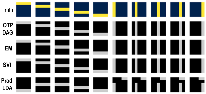
Figure 4: Topic-word distributions inferred by each method from the 1st set of synthetic data after 300 training epochs.

Topic Inference.

We now demonstrate the effectiveness of OTP-DAG on downstream applications. We here use OTP-DAG to infer the topics of $3$ real-world datasets: 20 News Group, BBC News and DBLP. We revert to the original generative process where the topic-word distribution follows a Dirichlet distribution parameterized by the concentration parameters $\beta$, instead of having $\gamma$ as a fixed quantity. $\beta$ is now initialized as a matrix of real values $\big{(}\beta\in\mathbb{R}^{K\times V}\big{)}$ representing the log concentration values.

For every topic $k$, we select top $10$ most related words according to $\gamma_{k}$ to represent it. Table 2 reports the quality of the inferred topics, which is evaluated via the diversity and coherence of the selected words. Diversity refers to the proportion of unique words, whereas Coherence is measured with normalized pointwise mutual information (Aletras & Stevenson, 2013), reflecting the extent to which the words in a topic are associated with a common theme. There exists a trade-off between Diversity and Coherence: words that are excessively diverse greatly reduce coherence, while a set of many duplicated words yields higher coherence yet harms diversity. A well-performing topic model would strike a good balance between these metrics. If we consider two metrics comprehensively, our method consistently achieves better performance across different settings. Qualitative results of the inferred topics can be found in Table 5.

Table 2: Coherence and Diversity of the inferred topics for the $3$ real-world datasets ($K=10$).

Metric (%) $\uparrow$	OTP-DAG (Ours)	Batch EM	SVI	Prod LDA
20 News Group
Coherence	10.45 $\pm$ 0.56	6.71 $\pm$ 0.16	5.90 $\pm$ 0.51	4.78 $\pm$ 2.64
Diversity	92.00 $\pm$ 2.65	72.33 $\pm$ 1.15	85.33 $\pm$ 5.51	92.67 $\pm$ 4.51
BBC News
Coherence	9.12 $\pm$ 0.81	8.67 $\pm$ 0.62	7.84 $\pm$ 0.49	2.17 $\pm$ 2.36
Diversity	86.67 $\pm$ 2.65	86.00 $\pm$ 1.00	92.33 $\pm$ 2.31	87.67 $\pm$ 3.79
DBLP
Coherence	7.66 $\pm$ 0.44	4.52 $\pm$ 0.53	1.47 $\pm$ 0.39	2.91 $\pm$ 1.70
Diversity	97.33 $\pm$ 1.53	81.33 $\pm$ 1.15	92.67 $\pm$ 2.52	98.67 $\pm$ 1.53

5.2 Hidden Markov Models

This application deals with time-series data following a Poisson hidden Markov model. Given a time series of $T$ steps, the task is to segment the data stream into 4 different states, each of which follows a Poisson distribution with rate $\lambda_{k}$ sampled from a Uniform hyper-prior. The observation at each step $t$ is given as

$$P(X_{t}|Z_{t}=k)=\mathrm{Poi}(X_{t}|\lambda_{k}),\quad\text{for}\ k=1,\cdots,4,$$

where $\lambda_{1}\sim U(10,20)$, $\lambda_{2}\sim U(30,40)$, $\lambda_{3}\sim U(50,60)$ and $\lambda_{4}\sim U(80,90)$. We further impose a uniform prior over the initial state. The Markov chain stays in the current state with probability $p$ and otherwise transitions to one of the other three states uniformly at random. The transition distribution is given as

$$Z_{1}\sim\mathrm{Cat}\bigg{(}\bigg{\{}\frac{1}{4},\frac{1}{4},\frac{1}{4},\frac{1}{4}\bigg{\}}\bigg{)},$$

$$Z_{t}|Z_{t-1}\sim\mathrm{Cat}\bigg{(}\left\{\begin{array}[]{lr}p&\text{if }Z_{t}=Z_{t-1}\\ \frac{1-p}{4-1}&\text{otherwise }\end{array}\right\}\bigg{)}$$

We randomly generate $200$ datasets of $50,000$ observations each. For each dataset, we train the models for $50$ epochs with learning rate of $0.05$ at $5$ different initializations. We would like to learn the concentration parameters $\lambda_{1:4}$ through which segmentation can be realized, assuming that the number of states is known. The other experimental configuration is reported in Appendix C.2.

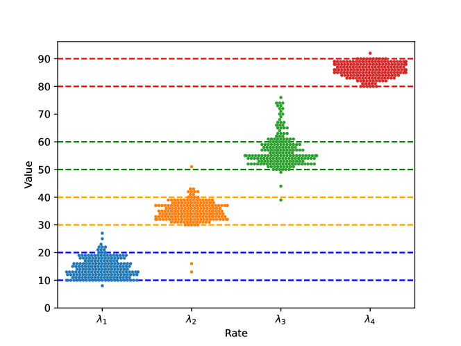
Figure 9: Distribution of the estimates of the concentration parameters $\lambda_{1:4}$ from OTP-DAG. Our estimated distribution uniformly aligns with the true generative process.

Table 3 reports mean error of the estimates of the parameters along with runtime of OTP-DAG and EM. Note that our method attempts to learn transition probability $p$ jointly with the error of $0.044\pm 0.027$ while for EM, we assume transition probability is known to increase the training time. EM thus only learns the concentration parameters, yet being much more timely expensive than OTP-DAG. Figure 9 additionally visualizes the distribution of our estimates to show the alignment with the generative uniform distributions.

Table 3: Estimates of the concentration parameters $\lambda_{1:4}$ of the Poisson HMM, measured by mean absolute error with the true values.

Method	OTP-DAG (Ours)	EM
$\lambda_{1}$	0.40 $\pm$ 1.29	0.22 $\pm$ 0.42
$\lambda_{2}$	0.80 $\pm$ 0.88	0.88 $\pm$ 1.05
$\lambda_{3}$	1.48 $\pm$ 1.19	1.47 $\pm$ 1.47
$\lambda_{4}$	0.84 $\pm$ 0.99	1.78 $\pm$ 1.40
Runtime ($50$ steps)	$\approx\mathbf{3}$ mins	$\approx 20$ mins

5.3 Learning Discrete Representations

Table 4: Quality of the image reconstructions from the vector quantized models ($K=512$).

Dataset	Method	Latent Size	SSIM $\uparrow$	PSNR $\uparrow$	LPIPS $\downarrow$	rFID $\downarrow$	Perplexity $\uparrow$
CIFAR10	VQ-VAE	8 $\times$ 8	0.70	23.14	0.35	77.3	69.8
	OTP-DAG (Ours)	8 $\times$ 8	0.80	25.40	0.23	56.5	498.6
MNIST	VQ-VAE	8 $\times$ 8	0.98	33.37	0.02	4.8	47.2
	OTP-DAG (Ours)	8 $\times$ 8	0.98	33.62	0.01	3.3	474.6
SVHN	VQ-VAE	8 $\times$ 8	0.88	26.94	0.17	38.5	114.6
	OTP-DAG (Ours)	8 $\times$ 8	0.94	32.56	0.08	25.2	462.8
CELEBA	VQ-VAE	16 $\times$ 16	0.82	27.48	0.19	19.4	48.9
	OTP-DAG (Ours)	16 $\times$ 16	0.88	29.77	0.11	13.1	487.5

Many types of data exist in discrete symbols e.g., words in texts, or pixels in images. This motivates the need to explore the latent discrete representations of the data, which can be useful for planning and symbolic reasoning tasks. Viewing discrete representation learning as a parameter learning problem, we endow it with a probabilistic generative process as illustrated in Figure 3. The problem deals with a latent space ${\mathcal{C}}\in\mathbb{R}^{K\times D}$ composed of $K$ discrete latent sub-spaces of $D$ dimensionality. The probability a data point belongs to a discrete sub-space $c\in\{1,\cdots,K\}$ follows a $K-$way categorical distribution $\pi=[\pi_{1},\cdots,\pi_{K}]$. In the language of VQ-VAE, each $c$ is referred to as a codeword and the set of codewords is called a codebook. Let $Z\in\mathbb{R}^{D}$ denote the latent variable in a sub-space. On each sub-space, we impose a Gaussian distribution parameterized by $\mu_{c},\Sigma_{c}$ where $\Sigma_{c}$ is diagonal. The generative process is as follows:

1. Sample $c\sim\textrm{Cat}(\pi)$ and $Z\sim{\mathcal{N}}(\mu_{c},\Sigma_{c})$

2. Quantize $\mu_{c}=Q(Z)$,

3. Generate $X=\psi_{\theta}(Z,\mu_{c})$,

where $\psi$ is a highly non-convex function with unknown parameters $\theta$ and often parameterized with a deep neural network. $Q$ refers to the quantization of $Z$ to $\mu_{c}$ defined as $\mu_{c}=Q(Z)$ where $c=\mathrm{argmin}_{c}\ d_{z}\big{(}Z;\mu_{c}\big{)}$ and $d_{z}=\sqrt{(Z-\mu_{c})^{T}\Sigma_{c}^{-1}(Z-\mu_{c})}$ is the Mahalanobis distance.

The goal is to learn the parameter set $\{\pi,\mu,\Sigma,\theta\}$ with $\mu=[\mu_{k}]_{k=1}^{K},\Sigma=[\Sigma_{k}]_{k=1}^{K}$ such that the learned representation captures the key properties of the data. Following VQ-VAE, our practical implementation considers $Z$ as an $M-$component latent embedding.

We experiment with images in this application and compare OTP-DAG with VQ-VAE on CIFAR10, MNIST, SVHN and CELEBA datasets. Since the true parameters are unknown, we assess how well the latent space characterizes the input data through the quality of the reconstruction of the original images. Table 4 reports our superior performance in preserving high-quality information of the input images. VQ-VAE suffers from poorer performance mainly due to codebook collapse (Yu et al., 2021) where most of latent vectors are quantized to limited discrete codewords. Meanwhile, our framework allows for control over the number of latent representations, ensuring all codewords are utilized. In Appendix C.3, we detail the formulation of our method and provide qualitative examples. We also showcase therein our competitive performance against a recent advance called SQ-VAE (Takida et al., 2022) without introducing any additional complexity.

6 Discussion and Conclusion

The key message across our experiments is that OTP-DAG is a scalable and versatile framework readily applicable to learning any directed graphs with latent variables. Similar to amortized VI, on one hand, our method employs amortized optimization and assumes one can sample from the priors or more generally, the model marginals over latent parents. OTP-DAG requires continuous relaxation through reparameterization of the underlying model distribution to ensure the gradients can be back-propagated effectively. Note that this specification is not unique to OTP-DAG: VAE also relies on reparameterization trick to compute the gradients w.r.t the variational parameters. For discrete distributions and for some continuous ones (e.g., Gamma distribution), this is not easy to attain. To this end, a proposal on Generalized Reparameterization Gradient (Ruiz et al., 2016) is a viable solution. On the other hand, different from VI, our global OT cost minimization is achieved by characterizing local densities through backward maps from the observed nodes to their parents. This localization strategy makes it easier to find a good approximation compared to VI, where the variational distribution is defined over all hidden variables and should ideally characterize the entire global dependencies in the graph. To model the backward distributions, we utilize the expressitivity of deep neural networks. Based on the universal approximation theorem (Hornik et al., 1989), the gap between the model distribution and the true conditional can be assumed to be smaller than an arbitrary constant $\epsilon$ given enough data, network complexity, and training time.

Future Research.

The proposed algorithm lays the cornerstone for an exciting paradigm shift in the realm of graphical learning and inference. Looking ahead, this fresh perspective unlocks a wealth of promising avenues for future application of OTP-DAG to large-scale inference problems or other learning tasks such as for undirected graphical models, or structural learning where edge existence and directionality can be parameterized as part of the model parameters.

Appendix A Proof

We now present the proof of Theorem 4.1 which is the key theorem in our paper.

Theorem 4.1. For every $\phi_{i}$ as defined above and fixed $\psi_{\theta}$,

$$W_{c}\big{(}P_{d}(X_{\mathbf{O}});P_{\theta}(X_{\mathbf{O}})\big{)}=\underset{\bigl{[}\phi_{i}\in\mathfrak{C}(X_{i})\bigr{]}_{i\in{\mathbf{O}}}}{\mathrm{inf}}\ \mathbb{E}_{X_{\mathbf{O}}\sim P_{d}(X_{\mathbf{O}}),\mathrm{PA}_{X_{\mathbf{O}}}\sim\phi(X_{\mathbf{O}})}\bigl{[}c\bigl{(}X_{\mathbf{O}},\psi_{\theta}(\mathrm{PA}_{X_{\mathbf{O}}})\bigr{)}\bigr{]},$$

where $\mathrm{PA}_{X_{\mathbf{O}}}:=\big{[}[X_{ij}]_{j\in\mathrm{PA}_{X_{i}}}\big{]}_{i\in{\mathbf{O}}}$.

Proof.

Let $\Gamma\in\mathcal{P}(P_{d}(X_{\mathbf{O}}),P_{\theta}(X_{\mathbf{O}}))$ be the optimal joint distribution over $P_{d}(X_{\mathbf{O}})$ and $P_{\theta}(X_{\mathbf{O}})$ of the corresponding Wasserstein distance. We consider three distributions: $P_{d}(X_{\mathbf{O}})$ over $A=\prod_{i\in\mathbf{O}}\mathcal{X}_{i}$, $P_{\theta}(X_{\mathbf{O}}))$ over $C=\prod_{i\in\mathbf{O}}\mathcal{X}_{i}$, and $P_{\theta}(\textrm{PA}_{X_{\mathbf{O}}})=P_{\theta}([\textrm{PA}_{X_{i}}]_{i\in\mathbf{O}})$ over $B=\prod_{i\in\mathbf{O}}\prod_{k\in\textrm{PA}_{X_{i}}}\mathcal{X}_{k}$. Here we note that the last distribution $P_{\theta}(\textrm{PA}_{X_{\mathbf{O}}})=P_{\theta}([\textrm{PA}_{X_{i}}]_{i\in\mathbf{O}})$ is the model distribution over the parent nodes of the observed nodes.

It is evident that $\Gamma\in\mathcal{P}(P_{d}(X_{\mathbf{O}}),P_{\theta}(X_{\mathbf{O}}))$ is a joint distribution over $P_{d}(X_{\mathbf{O}})$ and$P_{\theta}(X_{\mathbf{O}})$; let $\beta=(id,\psi_{\theta})\#P_{\theta}([\textrm{PA}_{X_{i}}]_{i\in\mathbf{O}})$ be a deterministic coupling or joint distribution over $P_{\theta}([\textrm{PA}_{X_{i}}]_{i\in\mathbf{O}})$ and $P_{\theta}(X_{\mathbf{O}})$. Using the gluing lemma (see Lemma 5.5 in (Santambrogio, 2015)), there exists a joint distribution $\alpha$ over $A\times B\times C$ such that $\alpha_{AC}=(\pi_{A},\pi_{C})\#\alpha=\Gamma$ and $\alpha_{BC}=(\pi_{B},\pi_{C})\#\alpha=\beta$ where $\pi$ is the projection operation. Let us denote $\gamma=(\pi_{A},\pi_{B})\#\alpha$ as a joint distribution over $P_{d}(X_{\mathbf{O}})$ and $P_{\theta}([\textrm{PA}_{X_{i}}]_{i\in\mathbf{O}})$.

Given $i\in\mathbf{O}$, we denote $\gamma_{i}$ as the projection of $\gamma$ over $\mathcal{X}_{i}$ and $\prod_{k\in\textrm{PA}_{X_{i}}}\mathcal{X}_{k}$. We further denote $\phi_{i}(X_{i})=\gamma_{i}(\cdot\mid X_{i})$ as a stochastic map from $\mathcal{X}_{i}$ to $\prod_{k\in\textrm{PA}_{X_{i}}}\mathcal{X}_{k}$. It is worth noting that because $\gamma_{i}$ is a joint distribution over $P_{d}(X_{i})$ and $P_{\theta}(\textrm{PA}_{X_{i}})$, $\phi_{i}\in\mathfrak{C}(X_{i})$.

$$W_{c}\left(P_{d}\left(X_{\mathbf{O}}\right),P_{\theta}\left(X_{\mathbf{O}}\right)\right) =\mathbb{E}_{\left(X_{\mathbf{O}},\tilde{X}_{\mathbf{O}}\right)\sim\Gamma}\left[c\left(X_{\mathbf{O}},\tilde{X}_{\mathbf{O}}\right)\right]=\mathbb{E}_{\left(X_{\mathbf{O}},\textrm{PA}_{X_{\mathbf{O}}},\tilde{X}_{\mathbf{O}}\right)\sim\alpha}\left[c\left(X_{\mathbf{O}},\tilde{X}_{\mathbf{O}}\right)\right]$$

$$= \mathbb{E}_{X_{\mathbf{O}}\sim P_{d},\left[\textrm{PA}_{X_{i}}\sim\gamma_{i}\left(\cdot\mid X_{i}\right)\right]_{i\in\mathbf{O}},\tilde{X}_{\mathbf{O}}\sim\alpha_{BC}\left(\cdot\mid\textrm{PA}_{X_{\mathbf{o}}}\right)}\left[c\left(X_{\mathbf{O}},\tilde{X}_{\mathbf{O}}\right)\right]$$

$$\overset{(1)}{=} \mathbb{E}_{X_{\mathbf{O}}\sim P_{d},\left[\textrm{PA}_{X_{i}}=\phi_{i}\left(X_{i}\right)\right]_{i\in\mathbf{O}},\tilde{X}_{\mathbf{O}}=\psi_{\theta}\left(\textrm{PA}_{X_{\mathbf{o}}}\right)}\left[c\left(X_{\mathbf{O}},\tilde{X}_{\mathbf{O}}\right)\right]$$

$$= \mathbb{E}_{X_{\mathbf{O}}\sim P_{d},\textrm{PA}_{X_{\mathbf{O}}}=\phi\left(X_{\mathbf{O}}\right),\tilde{X}_{\mathbf{O}}=\psi_{\theta}\left(\textrm{PA}_{X_{\mathbf{O}}}\right)}\left[c\left(X_{\mathbf{O}},\tilde{X}_{\mathbf{O}}\right)\right]$$

$$\overset{(2)}{=} \mathbb{E}_{X_{\mathbf{O}}\sim P_{d},\textrm{PA}_{X_{\mathbf{O}}}=\phi\left(X_{\mathbf{O}}\right)}\left[c\left(X_{\mathbf{O}},\psi_{\theta}\left(\textrm{PA}_{X_{\mathbf{O}}}\right)\right)\right]$$

$$\geq \inf_{\left[\phi_{i}\in\mathfrak{C}(X_{i})\right]_{i\in\mathbf{O}}}\mathbb{E}_{X_{\mathbf{O}}\sim P_{d},\textrm{PA}_{X_{\mathbf{O}}}=\phi\left(X_{\mathbf{O}}\right)}\left[c\left(X_{\mathbf{O}},\psi_{\theta}\left(\textrm{PA}_{X_{\mathbf{O}}}\right)\right)\right].$$ (4)

Here we note that we have $\overset{(1)}{=}$ because $\alpha_{BC}$ is a deterministic coupling and we have $\overset{(2)}{=}$ because the expectation is preserved through a deterministic push-forward map.

Let $[\phi_{i}\in\mathfrak{C}(X_{i})]_{i\in\mathbf{O}}$ be the optimal backward maps of the optimization problem (OP) in (A). We define the joint distribution $\gamma$ over $P_{d}\left(X_{\mathbf{O}}\right)$ and $P_{\theta}(\textrm{PA}_{X_{\mathbf{O}}})=P_{\theta}([\textrm{PA}_{X_{i}}]_{i\in\mathbf{O}})$ as follows. We first sample $X_{\mathbf{O}}\sim P_{d}(X_{\mathbf{O}})$ and for each $i\in\mathbf{O}$, we sample $\textrm{PA}_{X_{i}}\sim\phi_{i}(X_{i})$, and finally gather $(X_{\mathbf{O}},\textrm{PA}_{X_{\mathbf{O}}})\sim\gamma$ where $\textrm{PA}_{X_{\mathbf{O}}}=[\textrm{PA}_{X_{i}}]_{i\in\mathbf{O}}$. Consider the joint distribution $\gamma$ over $P_{d}\left(X_{\mathbf{O}}\right)$ , $P_{\theta}(\textrm{PA}_{X_{\mathbf{O}}})=P_{\theta}([\textrm{PA}_{X_{i}}]_{i\in\mathbf{O}})$ and the deterministic coupling or joint distribution $\beta=(id,\psi_{\theta})\#P_{\theta}([\textrm{PA}_{X_{i}}]_{i\in\mathbf{O}})$ over $P_{\theta}([\textrm{PA}_{X_{i}}]_{i\in\mathbf{O}})$ and $P_{\theta}(X_{\mathbf{O}})$, the gluing lemma indicates the existence of the joint distribution $\alpha$ over $A\times C\times B$ such that $\alpha_{AB}=(\pi_{A},\pi_{B})\#\alpha=\gamma$ and $\alpha_{BC}=(\pi_{B},\pi_{C})\#\alpha=\beta$. We further denote $\Gamma=\alpha_{AC}=(\pi_{A},\pi_{C})\#\alpha$ which is a joint distribution over $P_{d}(X_{\mathbf{O}})$ and $P_{\theta}(X_{\mathbf{O}})$. It follows that

$$\inf_{\left[\phi_{i}\in\mathfrak{C}(X_{i})\right]_{i\in\mathbf{O}}}\mathbb{E}_{X_{\mathbf{O}}\sim P_{d},\textrm{PA}_{X_{\mathbf{O}}}=\phi\left(X_{\mathbf{O}}\right)}\left[c\left(X_{\mathbf{O}},\psi_{\theta}\left(\textrm{PA}_{X_{\mathbf{O}}}\right)\right)\right]$$

$$= \mathbb{E}_{X_{\mathbf{O}}\sim P_{d},\textrm{PA}_{X_{\mathbf{O}}}=\phi\left(X_{\mathbf{O}}\right)}\left[c\left(X_{\mathbf{O}},\psi_{\theta}\left(\textrm{PA}_{X_{\mathbf{O}}}\right)\right)\right]$$

$$\overset{(1)}{=} \mathbb{E}_{X_{\mathbf{O}}\sim P_{d},\textrm{PA}_{X_{\mathbf{O}}}\sim\phi\left(X_{\mathbf{O}}\right),\tilde{X}_{\mathbf{O}}=\psi_{\theta}\left(\textrm{PA}_{X_{\mathbf{O}}}\right)}\left[c\left(X_{\mathbf{O}},\tilde{X}_{\mathbf{O}}\right)\right]$$

$$= \mathbb{E}_{X_{\mathbf{O}}\sim P_{d},\textrm{PA}_{X_{\mathbf{O}}}\sim\gamma\left(\cdot\mid X_{\mathbf{O}}\right),\tilde{X}_{\mathbf{O}}\sim\alpha_{BC}\left(\cdot\mid\textrm{PA}_{X_{\mathbf{o}}}\right)}\left[c\left(X_{\mathbf{O}},\tilde{X}_{\mathbf{O}}\right)\right]$$

$$= \mathbb{E}_{\left(X_{\mathbf{O}},\textrm{PA}_{X_{\mathbf{O}}},\tilde{X}_{\mathbf{O}}\right)\sim\alpha}\left[c\left(X_{\mathbf{O}},\tilde{X}_{\mathbf{O}}\right)\right]$$

$$= \mathbb{E}_{\left(X_{\mathbf{O}},\tilde{X}_{\mathbf{O}}\right)\sim\Gamma}\left[c\left(X_{\mathbf{O}},\tilde{X}_{\mathbf{O}}\right)\right]\geq W_{c}\left(P_{d}\left(X_{\mathbf{O}}\right),P_{\theta}\left(X_{\mathbf{O}}\right)\right).$$ (5)

Here we note that we have $\overset{(1)}{=}$ because the expectation is preserved through a deterministic push-forward map.

Finally, combining (4) and (5), we reach the conclusion. ∎

It is worth noting that according to Theorem 4.1, we need to solve the following OP:

$$\underset{\bigl{[}\phi_{i}\in\mathfrak{C}(X_{i})\bigr{]}_{i\in{\mathbf{O}}}}{\mathrm{inf}}\ \mathbb{E}_{X_{\mathbf{O}}\sim P_{d}(X_{\mathbf{O}}),\mathrm{PA}_{X_{\mathbf{O}}}\sim\phi(X_{\mathbf{O}})}\bigl{[}c\bigl{(}X_{\mathbf{O}},\psi_{\theta}(\mathrm{PA}_{X_{\mathbf{O}}})\bigr{)}\bigr{]},$$ (6)

where $\mathfrak{C}\left(X_{i}\right)=\left\{\phi_{i}:\phi_{i}\#P_{d}\left(X_{i}\right)=P_{\theta}\left(\mathrm{PA}_{X_{i}}\right)\right\},\forall i\in\mathbf{O}$.

If we make some further assumptions including: (i) the family model distributions $P_{\theta},\theta\in\Theta$ induced by the graphical model is sufficiently rich to contain the data distribution, meaning that there exist $\theta^{*}\in\Theta$ such that $P_{\theta^{*}}(X_{\mathbf{O}})=P_{d}(X_{\mathbf{O}})$ and (ii) the family of backward maps $\phi_{i},i\in\mathbf{O}$ has infinite capacity (i.e., they include all measure functions), the infimum really peaks $0$ at an optimal backward maps $\phi_{i}^{*},i\in\mathbf{O}$. We thus can replace the infimum by a minimization as

$$\underset{\bigl{[}\phi_{i}\in\mathfrak{C}(X_{i})\bigr{]}_{i\in{\mathbf{O}}}}{\mathrm{min}}\ \mathbb{E}_{X_{\mathbf{O}}\sim P_{d}(X_{\mathbf{O}}),\mathrm{PA}_{X_{\mathbf{O}}}\sim\phi(X_{\mathbf{O}})}\bigl{[}c\bigl{(}X_{\mathbf{O}},\psi_{\theta}(\mathrm{PA}_{X_{\mathbf{O}}})\bigr{)}\bigr{]}.$$ (7)

To make the OP in (7) tractable for training, we do relaxation as

$$\min_{\phi}\left\{\mathbb{E}_{X_{\mathbf{O}}\sim P_{d}(X_{\mathbf{O}}),\mathrm{PA}_{X_{\mathbf{O}}}\sim\phi(X_{\mathbf{O}})}\left[c\bigl{(}X_{\mathbf{O}},\psi_{\theta}(\mathrm{PA}_{X_{\mathbf{O}}})\bigr{)}\right]+\eta D\left(P_{\phi},P_{\theta}\left(\mathrm{PA}_{X_{\mathbf{O}}}\right)\right)\right\},$$ (8)

where $\eta>0$, $P_{\phi}$ is the distribution induced by the backward maps, and $D$ represents a general divergence. Here we note that $D\left(P_{\phi},P_{\theta}\left(\mathrm{PA}_{X_{\mathbf{O}}}\right)\right)$ can be decomposed into

$$D\left(P_{\phi},P_{\theta}\left(\mathrm{PA}_{X_{\mathbf{O}}}\right)\right)=\sum_{i\in\mathbf{O}}D_{i}\left(P_{\phi_{i}},P_{\theta}\left(\mathrm{PA}_{X_{\mathbf{i}}}\right)\right),$$

which is the sum of the divergences between the specific backward map distributions and their corresponding model distributions on the parent nodes (i.e., $P_{\phi_{i}}=\phi_{i}\#P_{d}\left(X_{i}\right)$). Additionally, in practice, using the WS distance for $D_{i}$ leads to the following OP

$$\min_{\phi}\left\{\mathbb{E}_{X_{\mathbf{O}}\sim P_{d}(X_{\mathbf{O}}),\mathrm{PA}_{X_{\mathbf{O}}}\sim\phi(X_{\mathbf{O}})}\left[c\bigl{(}X_{\mathbf{O}},\psi_{\theta}(\mathrm{PA}_{X_{\mathbf{O}}})\bigr{)}\right]+\eta\sum_{i\in\mathbf{O}}\textrm{W}_{c_{i}}\left(P_{\phi_{i}},P_{\theta}\left(\mathrm{PA}_{X_{i}}\right)\right)\right\}.$$ (9)

The following theorem characterizes the ability to search the optimal solutions for the OPs in (7), (8), and (9).

Theorem A.1.

Assume that the family model distributions $P_{\theta},\theta\in\Theta$ induced by the graphical model is sufficiently rich to contain the data distribution, meaning that there exist $\theta^{*}\in\Theta$ such that $P_{\theta^{*}}(X_{\mathbf{O}})=P_{d}(X_{\mathbf{O}})$ and the family of backward maps $\phi_{i},i\in\mathbf{O}$ has infinite capacity (i.e., they include all measure functions). The OPs in (7), (8), and (9) are equivalent and can obtain the common optimal solution.

Proof.

Let $\theta^{*}\in\Theta$ be the optimal solution such that $P_{\theta^{*}}(X_{\mathbf{O}})=P_{d}(X_{\mathbf{O}})$ and $W_{c}\left(P_{d}\left(X_{\mathbf{O}}\right),P_{\theta^{*}}\left(X_{\mathbf{O}}\right)\right)=0$. Let $\Gamma^{*}\in\mathcal{P}(P_{d}(X_{\mathbf{O}}),P_{\theta}(X_{\mathbf{O}}))$ be the optimal joint distribution over $P_{d}(X_{\mathbf{O}})$ and $P_{\theta}(X_{\mathbf{O}})$ of the corresponding Wasserstein distance, meaning that if $(X_{\mathbf{O}},\tilde{X}_{\mathbf{O}})\sim\Gamma^{*}$ then $X_{\mathbf{O}}=\tilde{X}_{\mathbf{O}}$. Using the gluing lemma as in the previous theorem, there exists a joint distribution $\alpha^{*}$ over $A\times B\times C$ such that $\alpha^{*}_{AC}=(\pi_{A},\pi_{C})\#\alpha^{*}=\Gamma^{*}$ and $\alpha^{*}_{BC}=(\pi_{B},\pi_{C})\#\alpha^{*}=\beta^{*}$ where $\beta^{*}=(id,\psi_{\theta})\#P_{\theta}^{*}([\textrm{PA}_{X_{i}}]_{i\in\mathbf{O}})$ is a deterministic coupling or joint distribution over $P_{\theta}([\textrm{PA}_{X_{i}}]_{i\in\mathbf{O}})$ and $P_{\theta}^{*}(X_{\mathbf{O}})$. This follows that $\alpha^{*}$ consists of the sample $(X_{\mathbf{O}},\mathrm{PA}_{X_{\mathbf{O}}},X_{\mathbf{O}})$ where $\psi_{\theta^{*}}(\mathrm{PA}_{X_{\mathbf{O}}})=X_{\mathbf{O}}$ with $X_{\mathbf{O}}\sim P_{d}(X_{\mathbf{O}})=P_{\theta}^{*}(X_{\mathbf{O}})$.

Let us denote $\gamma^{*}=(\pi_{A},\pi_{B})\#\alpha^{*}$ as a joint distribution over $P_{d}(X_{\mathbf{O}})$ and $P_{\theta}^{*}([\textrm{PA}_{X_{i}}]_{i\in\mathbf{O}})$. Let $\gamma_{i}^{*},i\in\mathbf{O}$ as the restriction of $\gamma^{*}$ over $P_{d}(X_{i})$ and $P_{\theta}^{*}(\textrm{PA}_{X_{i}})$. Let $\phi^{*}_{i},i\in\mathbf{O}$ be the functions in the family of the backward functions that can well-approximate $\gamma^{*}_{i},i\in\mathbf{O}$ (i.e., $\phi^{*}_{i}=\gamma^{*}_{i},i\in\mathbf{O}$). For any $X_{\mathbf{O}}\sim P_{d}(X_{\mathbf{O}})$, we have for all $i\in\mathbf{O}$, $\mathrm{PA}_{X_{i}}=\phi^{*}_{i}(X_{i})$ and $\psi_{\theta^{*}}(\mathrm{PA}_{X_{i}})=X_{i}$. These imply that (i) $\mathbb{E}_{X_{\mathbf{O}}\sim P_{d}(X_{\mathbf{O}}),\mathrm{PA}_{X_{\mathbf{O}}}\sim\phi^{*}(X_{\mathbf{O}})}\left[c\bigl{(}X_{\mathbf{O}},\psi_{\theta^{*}}(\mathrm{PA}_{X_{\mathbf{O}}})\bigr{)}\right]=0$ and (ii) $P_{\phi^{*}_{i}}=P_{\theta^{*}}\left(\mathrm{PA}_{X_{i}}\right),\forall i\in\mathbf{O}$, which further indicate that the OPs in (7), (8), and (9) are minimized at $0$ with the common optimal solution $\phi^{*}$ and $\theta^{*}$. ∎

Appendix B OTP-DAG as a generalization of WAE

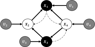
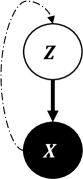
Figure 5: (Left) Algorithmic DAG. (Right) Standard Auto-encoder.

Figure 5 sheds light on an interesting connection of our method with auto-encoding models. Considering a graphical model of only two nodes: the observed node $X$ and its latent parent $Z$, we define a backward map $\phi$ over $X$ such that $\phi\#P_{d}(X)=P_{\theta}(Z)$ where $P_{\theta}(Z)$ is the prior over $Z$. The backward map can be viewed as a (stochastic) encoder approximating the prior $P_{\theta}(Z)$ with $P_{\phi}(Z):=\mathbb{E}_{X}[\phi(Z|X)]$. OTP-DAG now reduces to Wasserstein auto-encoder WAE (Tolstikhin et al., 2017), where the forward mapping $\psi$ plays the role of the decoder. OTP-DAG therefore serves as a generalization of WAE for learning a more complex structure where there is the interplay of more parameters and hidden variables. Note that WAE assumes $P(Z)$ is a Gaussian while our framework allows for the prior parameters to be optimized.

In this simplistic case, our training procedure is precisely as follows:

1. Draw $X\sim P_{d}(X)$.

2. Draw $Z\sim\phi(Z|X)$.

3. Draw $\widetilde{X}\sim P_{\theta}(X|Z)$.

4. Evaluate the costs according to Eq. 4 and update $\theta$.

Our cost function explicitly minimizes two terms: (1) the push-forward divergence $D[P_{\phi}(Z),P_{\theta}(Z)]$ where $D$ is an arbitrary divergence (we use the WS distance for $D$ in our experiments), and (2) the reconstruction loss between $X$ and $\widetilde{X}$.

Posterior Collapse.

Relaxing the push-forward constraint into the divergence term means the backward $\phi$ is forced to mimic the prior, which may lead to a situation similar to posterior collapse notoriously occurring to VAE. We here detail why VAE is prone to this issue and how the OT-based objective mitigates it.

Intuitively, our learning dynamic seeks to ensures $\phi_{\#}P_{d}(X)=P_{\phi}(Z)=P_{\theta}(Z)$ so that $Z\sim P_{\phi}(Z)$ follows the prior distribution $P_{\theta}(Z)$. However, such samples $Z\sim\phi(X)$ cannot ignore information in the input $X$ because we need $\widetilde{X}\sim P_{\theta}(X\mid Z)$ to effectively reconstruct $X\sim P_{d}(X)$, thus $\widetilde{X}$ should follow the data distribution $P_{d}(X)$.

1. The push-forward divergence

While the objectives of OTP-DAG/WAE and VAE entail the prior matching term. the two formulations are different in nature.

Let $Q$ denote the set of variational distributions. If we consider $\phi$ as an encoder, the VAE objective can be written as

$$\inf_{\phi(Z|X)\in Q}\mathbb{E}_{X\sim P(X)}[D_{\textrm{KL}}(\phi(Z|X),P_{\theta}(Z))]-\mathbb{E}_{Z\sim\phi(Z|X)}[\log P_{\theta}(X|Z)].$$ (10)

By minimizing the above KL divergence term, VAE basically tries to match the prior $P(Z)$ for all different examples drawn from $P_{d}(X)$. Under the VAE objective, it is thus easier for $\phi$ to collapse into a distribution independent of $P_{d}(X)$, where specifically latent codes are close to each other and reconstructed samples are concentrated around only few values.

For OTP-DAG/WAE, the regularizer in fact penalizes the discrepancy between $P_{\theta}(Z)$ and $P_{\phi}(Z):=\mathbb{E}_{X}[\phi(Z|X)]$, which can be optimized using GAN-based, MMD-based or Wasserstein distance. The latent codes of different examples $X\sim P_{d}(X)$ can lie far away from each other, which allows the model to maintain the dependency between the latent codes and the input. Therefore, it is more difficult for $\phi$ to mimic the prior and trivially satisfy the push-forward constraint. We refer readers to Tolstikhin et al. (2017) for extensive empirical evidence.

2. The reconstruction loss

At some point of training, there is still a possibility to land at $\phi$ that yields samples $Z$ independent of input $X$. If this occurs, $\phi\#\delta x^{(1)}_{c}=\phi\#\delta x^{(2)}_{c}=P(Z)$ for any points $x^{(1)}_{c},x^{(2)}_{c}\sim P_{d}(X)$. This means $\text{supp}(\phi(X^{1}))=\text{supp}(\phi(X^{2}))=\text{supp}(P_{\theta}(Z))$, so it would result in a very large reconstruction loss because it requires to map $\text{supp}(P_{\theta}(Z))$ to various $X^{1}$ and $X^{2}$. Thus our reconstruction term would heavily penalizes this. In other words, this term explicitly encourages the model to search for $\theta$ that reconstruct better, thus preventing the model from converging to the backward $\phi$ that produces sub-optimal ancestral samples.

Meanwhile, for VAE, if the family $Q$ contains all possible conditional distribution $\phi(Z|X)$, its objective is essentially to maximize the marginal log-likelihood $\mathbb{E}_{P(X)}[\log P_{\theta}(X)]$, or minimize the KL divergence $\text{KL}(P_{d},P_{\theta})$. It is shown in Dai et al. (2020) that under posterior collapse, VAE produces poor reconstructions yet the loss can still decrease i.e achieve low negative log-likelihood scores and still able to assign high-probability to the training data.

In summary, it is such construction and optimization of the backward that prevents OTP-DAG from posterior collapse situation. We here search for $\phi$ within a family of measurable functions and in practice approximate it with deep neural networks. It comes down to empirical decisions to select the architecture sufficiently expressive to each application.

Appendix C Experimental setup

In the following, we explain how OTP-DAG algorithm is implemented in practical applications, including how to reparameterize the model distribution, to design the backward mapping and to define the optimization objective. We also here provide the training configurations for our method and the baselines. All models are run on $4$ RTX 6000 GPU cores using Adam optimizer with a fixed learning rate of $1e-3$. Our code is anonymously published at https://anonymous.4open.science/r/OTP-7944/.

C.1 Latent Dirichlet Allocation

For completeness, let us recap the model generative process. We consider a corpus ${\mathcal{D}}$ of $M$ independent documents where each document is a sequence of $N$ words denoted by $W_{1:N}=(W_{1},W_{2},\cdots,W_{N})$. Documents are represented as random mixtures over $K$ latent topics, each of which is characterized by a distribution over words. Let $V$ be the size of a vocabulary indexed by $\{1,\cdots,V\}$. Latent Dirichlet Allocation (LDA) (Blei et al., 2003) dictates the following generative process for every document in the corpus:

1. Choose $\theta\sim\textrm{Dir}(\alpha)$,

2. Choose $\gamma_{k}\sim\textrm{Dir}(\beta)$ where $k\in\{1,\cdots,K\}$,

3. For each of the word positions $n\in\{1,\cdots,N\}$,

   • Choose a topic $z_{n}\sim\textrm{Multi-Nominal}(\theta)$,

   • Choose a word $w_{n}\sim\textrm{Multi-Nominal}(z_{n},\gamma_{k})$,

where $\textrm{Dir}(.)$ is a Dirichlet distribution, $\alpha<1$ and $\beta$ is typically sparse. $\theta$ is a $K-$dimensional vector that lies in the $(K-1)-$simplex and $\gamma_{k}$ is a $V-$dimensional vector represents the word distribution corresponding to topic $k$. Throughout the experiments, $K$ is fixed at $10$.

Parameter Estimation.

We consider the topic-word distribution $\gamma$ as a fixed quantity to be estimated. $\gamma$ is a $K\times V$ matrix where $\gamma_{kn}:=P(W_{n}=1|Z_{n}=1)$. The learnable parameters therefore consist of $\gamma$ and $\alpha$. An input document is represented with a $N\times V$ matrix where a word $W_{i}$ is represented with a one-hot $V-$vector such that the value at the index $i$ in the vocabulary is $1$ and $0$ otherwise. Given $\gamma\in[0,1]^{K\times V}$ and a selected topic $k$, the deterministic forward mapping to generate a document $W$ is defined as

$$W_{1:N}=\psi_{\gamma}(Z)=\text{Cat-Concrete}\big{(}\text{softmax}(Z^{\prime}\gamma)\big{)},$$

where $Z\in\{0,1\}^{K}$ is in the one-hot representation (i.e., $Z^{k}=1$ if state $k$ is the selected and $0$ otherwise) and $Z^{\prime}$ is its transpose. By applying the Gumbel-Softmax trick (Jang et al., 2016; Maddison et al., 2016), we re-parameterize the Categorical distribution into a function $\text{Cat-Concrete}(.)$ that takes the categorical probability vector (i.e., sum of all elements equals $1$) and output a relaxed probability vector. To be more specific, given a categorical variable of $K$ categories with probabilities $\big{[}p_{1},p_{2},...,p_{K}\big{]}$, for every the $\text{Cat-Concrete}(.)$ function is defined on each $p_{k}$ as

$$\text{Cat-Concrete}(p_{k})=\frac{\exp\big{\{}(\log p_{k}+G_{k})/\tau\big{\}}}{\sum^{K}_{k=1}\exp\big{\{}(\log p_{k}+G_{k})/\tau\big{\}}},$$

with temperature $\tau$, random noises $G_{k}$ independently drawn from Gumbel distribution $G_{t}=-\log(-\log u_{t}),\ u_{t}\sim\textrm{Uniform}(0,1)$.

We next define a backward map that outputs for a document a distribution over $K$ topics by $\phi(Z\mid W_{1:N})=\textrm{Cat}(Z).$

Given observations $W_{1:N}$, our learning procedure begins by sampling $\widetilde{Z}\sim\phi(Z|W_{1:N})$ and pass $\widetilde{Z}$ through the generative process given by $\psi$ to obtain the reconstruction. Notice here that we have a prior constraint over the distribution of $\theta$ i.e., $\theta$ follows a Dirichlet distribution parameterized by $\alpha$. This translates to a push forward constraint in order to optimize for $\alpha$. To facilitate differentiable training, we use softmax Laplace approximation (MacKay, 1998; Srivastava & Sutton, 2017) to approximate a Dirichlet distribution with a softmax Gaussian distribution. The relation between $\alpha$ and the Gaussian parameters $\big{(}\mu_{k},\Sigma_{k}\big{)}$ w.r.t a category $k$ where $\Sigma_{k}$ is a diagonal matrix is given as

$$\mu_{k}(\alpha)=\log\alpha_{k}-\frac{1}{K}\sum_{i=1}^{K}\log\alpha_{i},\quad\Sigma_{k}(\alpha)=\frac{1}{\alpha_{k}}\bigg{(}1-\frac{2}{K}\bigg{)}+\frac{1}{K^{2}}\sum_{i=1}^{K}\frac{1}{\alpha_{i}}.$$ (11)

Let us denote $P_{\alpha}:={\mathcal{N}}\big{(}\mu(\alpha),\Sigma(\alpha)\big{)}\approx\textrm{Dir}(\alpha)$ with $\mu=[\mu_{k}]_{k=1}^{K}$ and $\Sigma=[\Sigma_{k}]_{k=1}^{K}$ defined as above. We learn $\alpha,\gamma$ by minimizing the following optimization objective

$$\mathbb{E}_{W_{1:N},\widetilde{Z}}\bigg{[}c\big{(}W_{1:N},\psi_{\gamma}(\widetilde{Z})\big{)}+\eta\ D_{\textrm{WS}}\big{[}P_{\phi}(Z),P_{\alpha}\big{]}\bigg{]},$$

where $W_{1:N}\sim{\mathcal{D}}$, $\widetilde{Z}\sim\phi(Z\mid W_{1:N})$, $c$ is cross-entropy loss function and $D_{\textrm{WS}}$ is exact Wasserstein distance. The sampling process $\theta\sim P_{\alpha}$ is also relaxed using standard Gaussian reparameterization trick whereby $\theta=\mu(\alpha)+u\Sigma(\alpha)$ with $u\sim{\mathcal{N}}(0,1)$.

Remark.

Our framework in fact learns both $\alpha$ and $\gamma$ at the same time. Our estimates for $\alpha$ (averaged over $K$) are nearly $100\%$ faithful at $0.10,0.049,0.033$ (recall that the ground-truth $\alpha$ is uniform over $K$ where $K=10,20,30$ respectively). Figure 6 shows the convergence behavior of OTP-DAG during training where our model converges to the ground-truth patterns relatively quickly.

Figures 7 and 8 additionally present the topic distributions of each method for the second and third synthetic sets. We use horizontal and vertical patterns in different colors to distinguish topics from one another. Red circles indicate erroneous patterns. Note that these configurations are increasingly more complex, so it may require more training time for all methods to achieve better performance. Regardless, it is seen that although our method may exhibit some inconsistencies in recovering accurate word distributions for each topic, these discrepancies are comparatively less pronounced when compared to the baseline methods. This observation indicates a certain level of robustness in our approach.

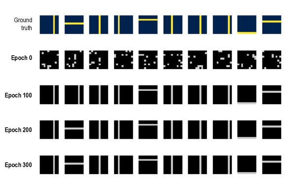
Figure 6: Converging patterns of $10$ random topics from our OTP-DAG after $100,200,300$ iterations.

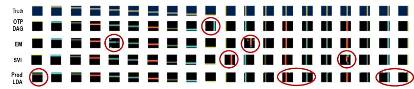
Figure 7: Topic-word distributions inferred by each method from the second set of synthetic data after 300 training epochs.

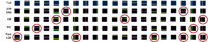
Figure 8: Topic-word distributions inferred by OTP-DAG from the third set of synthetic data after 300 training epochs.

Topic Inference.

In this experiment, we apply OTP-DAG on real-world topic modeling tasks. We here revert to the original generative process where the topic-word distribution follows a Dirichlet distribution parameterized by the concentration parameters $\beta$, instead of having $\gamma$ as a fixed quantity. In this case, $\beta$ is initialized as a matrix of real values i.e., $\beta\in\mathbb{R}^{K\times V}$ representing the log concentration values. The forward process is given as

$$W_{1:N}=\psi_{\gamma}(Z)=\text{Cat-Concrete}\big{(}\text{softmax}(Z^{\prime}\gamma)\big{)},$$

where $\gamma_{k}=\mu_{k}\big{(}\exp(\beta_{k})\big{)}+u_{k}\Sigma_{k}\big{(}\exp(\beta_{k})\big{)}$ and $u_{k}\sim{\mathcal{N}}(0,1)$ is a Gaussian noise. This is realized by using softmax Gaussian trick as in Eq. (11), then applying standard Gaussian reparameterization trick. The optimization procedure follows the previous application.

Table 5: Topics inferred for $3$ real-world datasets.

20 News Group
Topic 1	car, bike, front, engine, mile, ride, drive, owner, road, buy
Topic 2	game, play, team, player, season, fan, win, hit, year, score
Topic 3	government, public, key, clipper, security, encryption, law, agency, private, technology
Topic 4	religion, christian, belief, church, argument, faith, truth, evidence, human, life
Topic 5	window, file, program, software, application, graphic, display, user, screen, format
Topic 6	mail, sell, price, email, interested, sale, offer, reply, info, send
Topic 7	card, drive, disk, monitor, chip, video, speed, memory, system, board
Topic 8	kill, gun, government, war, child, law, country, crime, weapon, death
Topic 9	make, time, good, people, find, thing, give, work, problem, call
Topic 10	fire, day, hour, night, burn, doctor, woman, water, food, body
BBC News
Topic 1	rise, growth, market, fall, month, high, economy, expect, economic, price
Topic 2	win, play, game, player, good, back, match, team, final, side
Topic 3	user, firm, website, computer, net, information, software, internet, system, technology
Topic 4	technology, market, digital, high, video, player, company, launch, mobile, phone
Topic 5	election, government, party, labour, leader, plan, story, general, public, minister
Topic 6	film, include, star, award, good, win, show, top, play, actor
Topic 7	charge, case, face, claim, court, ban, lawyer, guilty, drug, trial
Topic 8	thing, work, part, life, find, idea, give, world, real, good
Topic 9	company, firm, deal, share, buy, business, market, executive, pay, group
Topic 10	government, law, issue, spokesman, call, minister, public, give, rule, plan
DBLP
Topic 1	learning, algorithm, time, rule, temporal, logic, framework, real, performance, function
Topic 2	efficient, classification, semantic, multiple, constraint, optimization, probabilistic, domain, process, inference
Topic 3	search, structure, pattern, large, language, web, problem, representation, support, machine
Topic 4	object, detection, application, information, method, estimation, multi, dynamic, tree, motion
Topic 5	system, database, query, knowledge, processing, management, orient, relational, expert, transaction
Topic 6	model, markov, mixture, variable, gaussian, topic, hide, latent, graphical, appearance
Topic 7	network, approach, recognition, neural, face, bayesian, belief, speech, sensor, artificial
Topic 8	base, video, content, code, coding, scalable, rate, streaming, frame, distortion
Topic 9	datum, analysis, feature, mining, cluster, selection, high, stream, dimensional, component
Topic 10	image, learn, segmentation, retrieval, color, wavelet, region, texture, transform, compression

Training Configuration.

The underlying architecture of the backward maps consists of an LSTM and one or more linear layers. We train all models for $300$ and $1,000$ epochs with batch size of $50$ respectively for the $2$ applications. We also set $\tau=1.0,2.0$ and $\eta=1e-4,1e-1$ respectively.

C.2 Hidden Markov Models

We here attempt to learn a Poisson hidden Markov model underlying a data stream. Given a time series ${\mathcal{D}}$ of $T$ steps, the task is to segment the data stream into $K$ different states, each of which is associated with a Poisson observation model with rate $\lambda_{k}$. The observation at each step $t$ is given as

$$P(X_{t}|Z_{t}=k)=\mathrm{Poi}(X_{t}|\lambda_{k}),\quad\text{for}\ k=1,\cdots,K.$$

The Markov chain stays in the current state with probability $p$ and otherwise transitions to one of the other $K-1$ states uniformly at random. The transition distribution is given as

$$Z_{1}\sim\mathrm{Cat}\bigg{(}\bigg{\{}\frac{1}{4},\frac{1}{4},\frac{1}{4},\frac{1}{4}\bigg{\}}\bigg{)},\quad Z_{t}|Z_{t-1}\sim\mathrm{Cat}\bigg{(}\left\{\begin{array}[]{lr}p&\text{if }Z_{t}=Z_{t-1}\\ \frac{1-p}{4-1}&\text{otherwise }\end{array}\right\}\bigg{)}$$

Let $P(Z_{1})$ and $P(Z_{t}|Z_{t-1})$ respectively denote these prior transition distributions. We first apply Gaussian reparameterization on each Poisson distribution, giving rise to a deterministic forward mapping

$$X_{t}=\psi_{t}(Z_{t})=Z^{\prime}_{t}\exp(\lambda)+u_{t}\sqrt{Z_{t}\exp(\lambda)},$$

where $\lambda\in\mathbb{R}^{K}$ is the learnable parameter vector representing log rates, $u_{k}\sim{\mathcal{N}}(0,1)$ is a Gaussian noise, $Z_{t}\in\{0,1\}^{K}$ is in the one-hot representation and $Z^{\prime}_{t}$ is its transpose. We define a global backward map $\phi$ that outputs the distributions for individual $Z_{t}$ as $\phi(X_{t}):=\mathrm{Cat}(Z_{t}).$

The first term in the optimization object is the reconstruction error given by a cost function $c$. The push forward constraint ensures the backward probabilities for the state variables align with the prior transition distributions. Putting everything together, we learn $\lambda_{1:K}$ by minimizing the following empirical objective

$$\mathbb{E}_{X_{1:T},\widetilde{Z}_{1:T}}\bigg{[}c\big{(}X_{1:T},\psi(\widetilde{Z}_{1:T})\big{)}+\eta\ D_{\textrm{WS}}\big{[}P_{\phi}(Z_{1}),P(Z_{1})\big{]}+\eta\ \sum_{t=2}^{T}D_{\textrm{WS}}\big{[}P_{\phi}(Z_{t}),P(Z_{t}|Z_{t-1})\big{]}\bigg{]},$$

where $X_{1:T}\sim{\mathcal{D}},\widetilde{Z}_{1:T}\sim\phi(Z_{1:T}|X_{1:T})$ and $\psi=[\psi_{t}]^{T}_{t=1}$.

In this application, $T=200$ and smooth $L_{1}$ loss (Girshick, 2015) is chosen as the cost function. $D_{\textrm{WS}}$ is exact Wasserstein distance with KL divergence as the ground cost.

Training Configuration.

The underlying architecture of the backward map is a $3-$ layer fully connected perceptron. The Poisson HMM is trained for $50$ epochs with $\eta=0.1$ and $\tau=0.1$.

C.3 Learning Discrete Representations

To understand vector quantized models, let us briefly review Quantization Variational Auto-Encoder (VQ-VAE) (Van Den Oord et al., 2017). The practical setting of VQ-VAE in fact considers a $M-$dimensional discrete latent space ${\mathcal{C}}^{M}\in\mathbb{R}^{M\times D}$ that is the $M-$ary Cartesian power of ${\mathcal{C}}$ with ${\mathcal{C}}=\{c_{k}\}_{k=1}^{K}\in\mathbb{R}^{K\times D}$ i.e., ${\mathcal{C}}$ here is the set of learnable latent embedding vectors $c_{k}$. The latent variable $Z=[Z^{m}]^{M}_{m=1}$ is an $M-$component vector where each component $Z^{m}\in{\mathcal{C}}$. VQ-VAE is an encoder-decoder, in which the encoder $f_{e}:{\mathcal{X}}\mapsto\mathbb{R}^{M\times D}$ maps the input data $X$ to the latent representation $Z$ and the decoder $f_{d}:\mathbb{R}^{M\times D}\mapsto{\mathcal{X}}$ reconstructs the input from the latent representation. However, different from standard VAE, the latent representation used for reconstruction is discrete, which is the projection of $Z$ onto ${\mathcal{C}}^{M}$ via the quantization process $Q$. Let $\bar{Z}$ denote the discrete representation. The quantization process is modeled as a deterministic categorical posterior distribution such that

$$\bar{Z}^{m}=Q(Z^{m})=c_{k},$$

where $k=\underset{k}{\textrm{argmin}}\ d\big{(}Z^{m},c_{k}\big{)}$, $Z^{m}=f^{m}_{e}(X)$ and $d$ is a metric on the latent space.

In our language, each vector $c_{k}$ can be viewed as the centroid representing each latent sub-space (or cluster). The quantization operation essentially searches for the closet cluster for every component latent representation $z^{m}$. VQ-VAE minimizes the following objective function:

$$\mathbb{E}_{x\sim{\mathcal{D}}}\bigg{[}d_{x}\big{[}f_{d}\big{(}Q(f_{e}(x))\big{)},x\big{]}+d_{z}\big{[}\textbf{sg}\big{(}f_{e}(x)\big{)},\bar{z}\big{]}+\beta d_{z}\big{[}f_{e}(x),\textbf{sg}\big{(}\bar{z}\big{)}\big{]}\bigg{]},$$

where ${\mathcal{D}}$ is the empirical data, sg is the stop gradient operation for continuous training, $d_{x},d_{z}$ are respectively the distances on the data and latent space and $\beta$ is set between $0.1$ and $2.0$ in the original proposal (Van Den Oord et al., 2017).

In our work, we explore a different model to learning discrete representations. Following VQ-VAE, we also consider $Z$ as a $M-$component latent embedding. On a $k^{th}$ sub-space (for $k\in\{1,\cdots,K\})$, we impose a Gaussian distribution parameterized by $\mu_{k},\Sigma_{k}$ where $\Sigma_{k}$ is diagonal. We also endow $M$ discrete distributions over $\mathbf{C}^{1},\dots,\mathbf{C}^{M}$, sharing a common support set as the set of sub-spaces induced by $\{(\mu_{k},\Sigma_{k})\}_{k=1}^{K}$:

$$\mathbb{P}_{k,\pi^{m}}=\sum_{k=1}^{K}\pi_{k}^{m}\delta_{\mu_{k}},\ \text{for }m=1,\dots,M.$$

with the Dirac delta function $\delta$ and the weights $\pi^{m}\in\Delta_{K-1}=\{\alpha\geq\bm{0}:\|\alpha\|_{1}=1\}$ in the $(K-1)$-simplex. The probability a data point $z^{m}$ belongs to a discrete $k^{th}$ sub-space follows a $K-$way categorical distribution $\pi^{m}=[\pi^{m}_{1},\cdots,\pi^{m}_{K}]$. In such a practical setting, the generative process is detailed as follows

1. For $m\in\{1,\cdots,M\}$,

   • Sample $k\sim\textrm{Cat}(\pi^{m})$,

   • Sample $z^{m}\sim{\mathcal{N}}(\mu_{k},\Sigma_{k})$,

   • Quantize $\mu^{m}_{k}=Q(z^{m})$,

2. $x=\psi_{\theta}([z^{m}]_{m=1}^{M},[\mu^{m}_{k}]_{m=1}^{M})$.

where $\psi$ is a highly non-convex function with unknown parameters $\theta$. $Q$ refers to the quantization of $[z^{m}]_{m=1}^{M}$ to $[\mu^{m}_{k}]_{m=1}^{M}$ defined as $\mu^{m}_{k}=Q(z^{m})$ where $k=\mathrm{argmin}_{k}\ d_{z}\big{(}z^{m};\mu_{k}\big{)}$ and $d_{z}=\sqrt{(z^{m}-\mu_{k})^{T}\Sigma_{k}^{-1}(z^{m}-\mu_{k})}$ is the Mahalanobis distance.

The backward map is defined via an encoder function $f_{e}$ and quantization process $Q$ as

$$\phi(x)=\big{[}f_{e}(x),Q(f_{e}(x))\big{]},\quad z=[z^{m}]_{m=1}^{M}=f_{e}(x),\quad[\mu^{m}_{k}]_{m=1}^{M}=Q(z).$$

The learnable parameters are $\{\pi,\mu,\Sigma,\theta\}$ with $\pi=[[\pi^{m}_{k}]_{m=1}^{M}]_{k=1}^{K},\mu=[\mu_{k}]_{k=1}^{K},\Sigma=[\Sigma_{k}]_{k=1}^{K}$.

Applying OTP-DAG to the above generative model yields the following optimization objective:

$$\underset{\pi,\mu,\Sigma,\theta}{\mathrm{min}} \quad\mathbb{E}_{X\sim{\mathcal{D}}}\bigg{[}c\big{[}X,\psi_{\theta}(Z,\mu_{k})\big{]}\bigg{]}+\frac{\eta}{M}\ \sum_{m=1}^{M}\big{[}D_{\textrm{WS}}\big{(}P_{\phi}(Z^{m}),P(\widetilde{Z}^{m})\big{)}+D_{\textrm{WS}}\big{(}P_{\phi}(Z^{m}),\mathbb{P}_{k,\pi^{m}}\big{)}\big{]}$$

$$+\eta_{r}\ \sum^{M}_{m=1}D_{\textrm{KL}}\big{(}\pi^{m},{\mathcal{U}}_{K}\big{)},$$

where $P_{\phi}(Z^{m}):=f_{e}^{m}\#P(X)$ given by the backward $\phi$, $P(\widetilde{Z}^{m})=\sum^{K}_{k=1}\pi^{m}_{k}{\mathcal{N}}(\widetilde{Z}^{m}|\mu_{k},\Sigma_{k})$ is the mixture of Gaussian distributions. The copy gradient trick (Van Den Oord et al., 2017) is applied throughout to facilitate backpropagation.

The first term is the conventional reconstruction loss where $c$ is chosen to be mean squared error. Minimizing the second term $D_{\textrm{WS}}\big{(}P_{\phi}(Z^{m}),P(\widetilde{Z}^{m})\big{)}$ forces the latent representations to follow the Gaussian distribution ${\mathcal{N}}(\mu^{m}_{k},\Sigma^{m}_{k})$. Minimizing the third term $D_{\textrm{WS}}\big{(}P_{\phi}(Z^{m}),\mathbb{P}_{k,\pi^{m}}\big{)}$ encourages every $\mu_{k}$ to become the clustering centroid of the set of latent representations $Z^{m}$ associated with it. Additionally, the number of latent representations associated with the clustering centroids are proportional to $\pi^{m}_{k},k=1,...,K$. Therefore, we use the fourth term $\sum^{M}_{m=1}D_{\textrm{KL}}\big{(}\pi^{m},{\mathcal{U}}_{K}\big{)}$ to guarantee every centroid is utilized.

Training Configuration.

We use the same experiment setting on all datasets. The models have an encoder with two convolutional layers of stride $2$ and filter size of $4\times 4$ with ReLU activation, followed by $2$ residual blocks, which contained a $3\times 3,$ stride $1$ convolutional layer with ReLU activation followed by a $1\times 1$ convolution. The decoder was similar, with two of these residual blocks followed by two de-convolutional layers. The hyperparameters are: $D=M=64,K=512,\eta=1e-3,\eta_{r}=1.0$, batch size of $32$ and $100$ training epochs.

Evaluation Metrics.

The evaluation metrics used include (1) SSIM: the patch-level structure similarity index, which evaluates the similarity between patches of the two images; (2) PSNR: the pixel-level peak signal-to-noise ratio, which measures the similarity between the original and generated image at the pixel level; (3) feature-level LPIPS (Zhang et al., 2018), which calculates the distance between the feature representations of the two images; (4) the dataset-level Fr’echlet Inception Distance (FID) (Heusel et al., 2017), which measures the difference between the distributions of real and generated images in a high-dimensional feature space; and (5) Perplexity: the degree to which the latent representations $Z$ spread uniformly over $K$ sub-spaces i.e., all $K$ regions are occupied.

Additional Experiment.

We additionally investigate a recent model called SQ-VAE (Takida et al., 2022) proposed to tackle the issue of codebook utilization. Table 6 reports the performance of SQ-VAE in comparison with our OTP-DAG. We significantly outperform SQ-VAE on Perplexity, showing that our model mitigates codebook collapse issue more effectively, while compete on par with this SOTA model across the other metrics. It is worth noting that our goal here is not to propose any SOTA model to discrete representation learning, but rather to demonstrate the applicability of OTP-DAG on various tasks, particular problems where traditional methods such as EM or mean-field VI cannot simply tackle.

Qualitative Examples.

We first present the generated samples from the CelebA dataset using Image transformer (Parmar et al., 2018) as the generative model. From Figure 10, it can be seen that the discrete representation from the our method can be effectively utilized for image generation with acceptable quality.

We additionally show the reconstructed samples from CIFAR10 dataset for qualitative evaluation. Figures 13-13 illustrate that the reconstructions from OTP-DAG have higher visual quality than VQ-VAE. The high-level semantic features of the input image and colors are better preserved with OTP-DAG than VQ-VAE from which some reconstructed images are much more blurry.

Table 6: Quality of image reconstructions

Dataset	Method	Latent Size	SSIM $\uparrow$	PSNR $\uparrow$	LPIPS $\downarrow$	rFID $\downarrow$	Perplexity $\uparrow$
CIFAR10	SQ-VAE	8 $\times$ 8	0.80	26.11	0.23	55.4	434.8
	OTP-DAG (Ours)	8 $\times$ 8	0.80	25.40	0.23	56.5	498.6
MNIST	SQ-VAE	8 $\times$ 8	0.99	36.25	0.01	3.2	301.8
	OTP-DAG (Ours)	8 $\times$ 8	0.98	33.62	0.01	3.3	474.6
SVHN	SQ-VAE	8 $\times$ 8	0.96	35.35	0.06	24.8	389.8
	OTP-DAG (Ours)	8 $\times$ 8	0.94	32.56	0.08	25.2	462.8
CELEBA	SQ-VAE	16 $\times$ 16	0.88	31.05	0.12	14.8	427.8
	OTP-DAG (Ours)	16 $\times$ 16	0.88	29.77	0.11	13.1	487.5

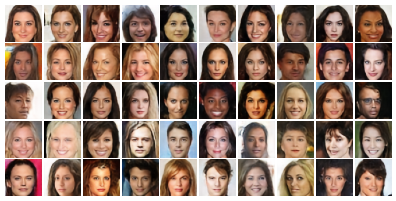
Figure 10: Generated images from the discrete representations of OTP-DAG on CelebA dataset.

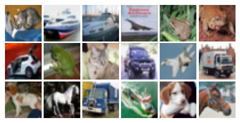
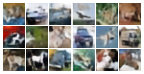
Figure 11: Original CIFAR10 images.

Figure 12: Random reconstructed images by VQ-VAE from CIFAR10 dataset.

Figure 13: Random reconstructed images by OTP-DAG from CIFAR10 dataset.

References

- Adler & Lunz (2018) Adler, J. and Lunz, S. Banach wasserstein gan. Advances in neural information processing systems, 31, 2018.
- Aletras & Stevenson (2013) Aletras, N. and Stevenson, M. Evaluating topic coherence using distributional semantics. In Proceedings of the 10th international conference on computational semantics (IWCS 2013)–Long Papers, pp. 13–22, 2013.
- Ambrogioni et al. (2018) Ambrogioni, L., Güçlü, U., Güçlütürk, Y., Hinne, M., Van Gerven, M. A., and Maris, E. Wasserstein variational inference. Advances in Neural Information Processing Systems, 2018-December(NeurIPS):2473–2482, 2018. ISSN 10495258.
- Ambrogioni et al. (2021) Ambrogioni, L., Lin, K., Fertig, E., Vikram, S., Hinne, M., Moore, D., and van Gerven, M. Automatic structured variational inference. In Banerjee, A. and Fukumizu, K. (eds.), Proceedings of The 24th International Conference on Artificial Intelligence and Statistics, volume 130 of Proceedings of Machine Learning Research, pp. 676–684. PMLR, 13–15 Apr 2021. URL https://proceedings.mlr.press/v130/ambrogioni21a.html.
- Amos (2022) Amos, B. Tutorial on amortized optimization for learning to optimize over continuous domains. arXiv preprint arXiv:2202.00665, 2022.
- Anandkumar et al. (2012) Anandkumar, A., Hsu, D., and Kakade, S. M. A method of moments for mixture models and hidden markov models. In Conference on Learning Theory, pp. 33–1. JMLR Workshop and Conference Proceedings, 2012.
- Anandkumar et al. (2014) Anandkumar, A., Ge, R., Hsu, D., Kakade, S. M., and Telgarsky, M. Tensor decompositions for learning latent variable models. Journal of machine learning research, 15:2773–2832, 2014.
- Arjovsky et al. (2017) Arjovsky, M., Chintala, S., and Bottou, L. Wasserstein generative adversarial networks. In International conference on machine learning, pp. 214–223. PMLR, 2017.
- Bassetti et al. (2006) Bassetti, F., Bodini, A., and Regazzini, E. On minimum kantorovich distance estimators. Statistics & probability letters, 76(12):1298–1302, 2006.
- Beal & Ghahramani (2006) Beal, M. J. and Ghahramani, Z. Variational bayesian learning of directed graphical models with hidden variables. 2006.
- Bernton et al. (2019) Bernton, E., Jacob, P. E., Gerber, M., and Robert, C. P. On parameter estimation with the wasserstein distance. Information and Inference: A Journal of the IMA, 8(4):657–676, 2019.
- Bishop & Nasrabadi (2006) Bishop, C. M. and Nasrabadi, N. M. Pattern recognition and machine learning, volume 4. Springer, 2006.
- Blei et al. (2003) Blei, D. M., Ng, A. Y., and Jordan, M. I. Latent dirichlet allocation. Journal of machine Learning research, 3(Jan):993–1022, 2003.
- Cappé & Moulines (2009) Cappé, O. and Moulines, E. On-line expectation–maximization algorithm for latent data models. Journal of the Royal Statistical Society: Series B (Statistical Methodology), 71(3):593–613, 2009.
- Dai et al. (2020) Dai, B., Wang, Z., and Wipf, D. The usual suspects? reassessing blame for vae posterior collapse. In International conference on machine learning, pp. 2313–2322. PMLR, 2020.
- Delyon et al. (1999) Delyon, B., Lavielle, M., and Moulines, E. Convergence of a stochastic approximation version of the em algorithm. Annals of statistics, pp. 94–128, 1999.
- Dempster et al. (1977) Dempster, A. P., Laird, N. M., and Rubin, D. B. Maximum Likelihood from Incomplete Data Via the EM Algorithm . Journal of the Royal Statistical Society: Series B (Methodological), 39(1):1–22, 1977. doi: 10.1111/j.2517-6161.1977.tb01600.x.
- Foti et al. (2014) Foti, N., Xu, J., Laird, D., and Fox, E. Stochastic variational inference for hidden markov models. Advances in neural information processing systems, 27, 2014.
- Gelfand & Smith (1990) Gelfand, A. E. and Smith, A. F. Sampling-based approaches to calculating marginal densities. Journal of the American statistical association, 85(410):398–409, 1990.
- Gilks et al. (1995) Gilks, W. R., Richardson, S., and Spiegelhalter, D. Markov chain Monte Carlo in practice. CRC press, 1995.
- Girshick (2015) Girshick, R. Fast r-cnn. In Proceedings of the IEEE international conference on computer vision, pp. 1440–1448, 2015.
- Griffiths & Steyvers (2004) Griffiths, T. L. and Steyvers, M. Finding scientific topics. Proceedings of the National academy of Sciences, 101(suppl_1):5228–5235, 2004.
- Hammersley (2013) Hammersley, J. Monte carlo methods. Springer Science & Business Media, 2013.
- Hellinger (1909) Hellinger, E. Neue begründung der theorie quadratischer formen von unendlichvielen veränderlichen. Journal für die reine und angewandte Mathematik, 1909(136):210–271, 1909.
- Hensman et al. (2012) Hensman, J., Rattray, M., and Lawrence, N. Fast variational inference in the conjugate exponential family. Advances in neural information processing systems, 25, 2012.
- Hernandez-Lobato et al. (2016) Hernandez-Lobato, J., Li, Y., Rowland, M., Bui, T., Hernández-Lobato, D., and Turner, R. Black-box alpha divergence minimization. In International conference on machine learning, pp. 1511–1520. PMLR, 2016.
- Heusel et al. (2017) Heusel, M., Ramsauer, H., Unterthiner, T., Nessler, B., and Hochreiter, S. Gans trained by a two time-scale update rule converge to a local nash equilibrium. Advances in neural information processing systems, 30, 2017.
- Ho et al. (2017) Ho, N., Nguyen, X., Yurochkin, M., Bui, H. H., Huynh, V., and Phung, D. Multilevel clustering via wasserstein means. In International conference on machine learning, pp. 1501–1509. PMLR, 2017.
- Hoffman & Blei (2015) Hoffman, M. D. and Blei, D. M. Structured stochastic variational inference. In Artificial Intelligence and Statistics, pp. 361–369, 2015.
- Hoffman et al. (2013) Hoffman, M. D., Blei, D. M., Wang, C., and Paisley, J. Stochastic variational inference. Journal of Machine Learning Research, 2013.
- Hornik et al. (1989) Hornik, K., Stinchcombe, M., and White, H. Multilayer feedforward networks are universal approximators. Neural networks, 2(5):359–366, 1989.
- Jang et al. (2016) Jang, E., Gu, S., and Poole, B. Categorical reparameterization with gumbel-softmax. arXiv preprint arXiv:1611.01144, 2016.
- Johnson & Willsky (2014) Johnson, M. and Willsky, A. Stochastic variational inference for bayesian time series models. In International Conference on Machine Learning, pp. 1854–1862. PMLR, 2014.
- Jordan et al. (1999) Jordan, M. I., Ghahramani, Z., Jaakkola, T. S., and Saul, L. K. An introduction to variational methods for graphical models. Machine learning, 37:183–233, 1999.
- Kantorovich (1960) Kantorovich, L. V. Mathematical methods of organizing and planning production. Management science, 6(4):366–422, 1960.
- King & Lawrence (2006) King, N. J. and Lawrence, N. D. Fast variational inference for gaussian process models through kl-correction. In Machine Learning: ECML 2006: 17th European Conference on Machine Learning Berlin, Germany, September 18-22, 2006 Proceedings 17, pp. 270–281. Springer, 2006.
- Kingma et al. (2016) Kingma, D. P., Salimans, T., Jozefowicz, R., Chen, X., Sutskever, I., and Welling, M. Improved variational inference with inverse autoregressive flow. Advances in neural information processing systems, 29, 2016.
- Kolouri et al. (2018) Kolouri, S., Rohde, G. K., and Hoffmann, H. Sliced wasserstein distance for learning gaussian mixture models. In Proceedings of the IEEE Conference on Computer Vision and Pattern Recognition, pp. 3427–3436, 2018.
- Lázaro-Gredilla et al. (2012) Lázaro-Gredilla, M., Van Vaerenbergh, S., and Lawrence, N. D. Overlapping mixtures of gaussian processes for the data association problem. Pattern recognition, 45(4):1386–1395, 2012.
- Li & Turner (2016) Li, Y. and Turner, R. E. Rényi divergence variational inference. Advances in neural information processing systems, 29, 2016.
- Liang & Klein (2009) Liang, P. and Klein, D. Online em for unsupervised models. In Proceedings of human language technologies: The 2009 annual conference of the North American chapter of the association for computational linguistics, pp. 611–619, 2009.
- MacKay (1998) MacKay, D. J. Choice of basis for laplace approximation. Machine learning, 33:77–86, 1998.
- Maddison et al. (2016) Maddison, C. J., Mnih, A., and Teh, Y. W. The concrete distribution: A continuous relaxation of discrete random variables. arXiv preprint arXiv:1611.00712, 2016.
- Mena et al. (2020) Mena, G., Nejatbakhsh, A., Varol, E., and Niles-Weed, J. Sinkhorn em: an expectation-maximization algorithm based on entropic optimal transport. arXiv preprint arXiv:2006.16548, 2020.
- Molchanov et al. (2019) Molchanov, D., Kharitonov, V., Sobolev, A., and Vetrov, D. Doubly semi-implicit variational inference. In The 22nd International Conference on Artificial Intelligence and Statistics, pp. 2593–2602. PMLR, 2019.
- Neal & Hinton (1998) Neal, R. M. and Hinton, G. E. A view of the em algorithm that justifies incremental, sparse, and other variants. Learning in graphical models, pp. 355–368, 1998.
- Neath et al. (2013) Neath, R. C. et al. On convergence properties of the monte carlo em algorithm. Advances in modern statistical theory and applications: a Festschrift in Honor of Morris L. Eaton, pp. 43–62, 2013.
- Papamakarios et al. (2021) Papamakarios, G., Nalisnick, E., Rezende, D. J., Mohamed, S., and Lakshminarayanan, B. Normalizing flows for probabilistic modeling and inference. Journal of Machine Learning Research, 22:1–64, 2021. ISSN 15337928.
- Parmar et al. (2018) Parmar, N., Vaswani, A., Uszkoreit, J., Kaiser, L., Shazeer, N., Ku, A., and Tran, D. Image transformer. In International conference on machine learning, pp. 4055–4064. PMLR, 2018.
- Peyré et al. (2017) Peyré, G., Cuturi, M., et al. Computational optimal transport. Center for Research in Economics and Statistics Working Papers, (2017-86), 2017.
- Ranganath et al. (2014) Ranganath, R., Gerrish, S., and Blei, D. Black box variational inference. In Artificial intelligence and statistics, pp. 814–822. PMLR, 2014.
- Ranganath et al. (2016) Ranganath, R., Tran, D., and Blei, D. Hierarchical variational models. In International conference on machine learning, pp. 324–333. PMLR, 2016.
- Ruiz et al. (2016) Ruiz, F. R., AUEB, T. R., Blei, D., et al. The generalized reparameterization gradient. Advances in neural information processing systems, 29, 2016.
- Santambrogio (2015) Santambrogio, F. Optimal transport for applied mathematicians. Birkäuser, NY, 55(58-63):94, 2015.
- Saul & Jordan (1995) Saul, L. and Jordan, M. Exploiting tractable substructures in intractable networks. Advances in neural information processing systems, 8, 1995.
- Srivastava & Sutton (2017) Srivastava, A. and Sutton, C. Autoencoding variational inference for topic models. arXiv preprint arXiv:1703.01488, 2017.
- Takida et al. (2022) Takida, Y., Shibuya, T., Liao, W., Lai, C.-H., Ohmura, J., Uesaka, T., Murata, N., Takahashi, S., Kumakura, T., and Mitsufuji, Y. Sq-vae: Variational bayes on discrete representation with self-annealed stochastic quantization. In International Conference on Machine Learning, pp. 20987–21012. PMLR, 2022.
- Teh et al. (2006) Teh, Y., Newman, D., and Welling, M. A collapsed variational bayesian inference algorithm for latent dirichlet allocation. Advances in neural information processing systems, 19, 2006.
- Titsias & Ruiz (2019) Titsias, M. K. and Ruiz, F. Unbiased implicit variational inference. In The 22nd International Conference on Artificial Intelligence and Statistics, pp. 167–176. PMLR, 2019.
- Tolstikhin et al. (2017) Tolstikhin, I., Bousquet, O., Gelly, S., and Schoelkopf, B. Wasserstein auto-encoders. arXiv preprint arXiv:1711.01558, 2017.
- Tran et al. (2015) Tran, D., Blei, D., and Airoldi, E. M. Copula variational inference. Advances in neural information processing systems, 28, 2015.
- Van Den Oord et al. (2017) Van Den Oord, A., Vinyals, O., et al. Neural discrete representation learning. Advances in neural information processing systems, 30, 2017.
- Villani et al. (2009) Villani, C. et al. Optimal transport: old and new, volume 338. Springer, 2009.
- Wan et al. (2020) Wan, N., Li, D., and Hovakimyan, N. F-divergence variational inference. Advances in neural information processing systems, 33:17370–17379, 2020.
- Wei & Tanner (1990) Wei, G. C. and Tanner, M. A. A monte carlo implementation of the em algorithm and the poor man’s data augmentation algorithms. Journal of the American statistical Association, 85(411):699–704, 1990.
- Xu et al. (2019) Xu, M., Quiroz, M., Kohn, R., and Sisson, S. A. Variance reduction properties of the reparameterization trick. In The 22nd International Conference on Artificial Intelligence and Statistics, pp. 2711–2720. PMLR, 2019.
- Yin & Zhou (2018) Yin, M. and Zhou, M. Semi-implicit variational inference. In International Conference on Machine Learning, pp. 5660–5669. PMLR, 2018.
- Yu et al. (2021) Yu, J., Li, X., Koh, J. Y., Zhang, H., Pang, R., Qin, J., Ku, A., Xu, Y., Baldridge, J., and Wu, Y. Vector-quantized image modeling with improved vqgan. arXiv preprint arXiv:2110.04627, 2021.
- Zhang et al. (2018) Zhang, R., Isola, P., Efros, A. A., Shechtman, E., and Wang, O. The unreasonable effectiveness of deep features as a perceptual metric. In Proceedings of the IEEE conference on computer vision and pattern recognition, pp. 586–595, 2018.