Double Descent of Discrepancy:
A Task-, Data-, and Model-Agnostic Phenomenon

Abstract

In this paper, we studied two identically-trained neural networks (i.e. networks with the same architecture, trained on the same dataset using the same algorithm, but with different initialization) and found that their outputs discrepancy on the training dataset exhibits a "double descent" phenomenon. We demonstrated through extensive experiments across various tasks, datasets, and network architectures that this phenomenon is prevalent. Leveraging this phenomenon, we proposed a new early stopping criterion and developed a new method for data quality assessment. Our results show that a phenomenon-driven approach can benefit deep learning research both in theoretical understanding and practical applications.

1 Introduction

The methodology of observing phenomena, formulating hypotheses, designing experiments, and drawing conclusions is fundamental to scientific progress. This phenomenon-driven paradigm has led to breakthroughs in fields ranging from physics to biology that have reshaped our understanding of the world. However, this paradigm is less observed in the field of deep learning.

Modern deep learning has achieved remarkable practical successes, yet our theoretical understanding of deep neural networks (DNNs) remains limited. As deep learning continues its rapid progress, applying a scientific, phenomenon-driven approach is crucial to gaining a deeper understanding of the field. Rather than relying solely on preconceived theories, phenomenon-driven approach allows the models to speak for themselves, revealing new insights that often yield surprises. Since phenomenon-driven discoveries originate from real observations, their results also tend to be more informative to practice.

The significance of phenomenon-driven approach is amplified as DNN models grow increasingly complex. For massive models like Large Language Models with billions of parameters, understanding from theoretical principles alone is implausible. However, by observing phenomena, formulating hypotheses, and test them through designed experiments, we can obtain some solid conclusions that can serve as the basis for future theories.

There have been some works that embody this approach. Here we introduce two notable examples: double descent and frequency principles.

Double descent. As reported in [1, 2], the "double descent" phenomenon refers to the observation that as model size increases, model generalization ability first gets worse but then gets better, contradicting the usual belief that overparameterization leads to overfitting. This phenomenon provides a new perspective on understanding the generalization ability of overparameterized DNNs [3, 4, 5, 6]. It also provides a useful guidance on how to balance data size and model size.

Frequency principles. According to [7, 8], the "frequency principle" or "spectral bias" refers to the observation that DNNs often learn target functions from low to high frequencies during training. This bias is contrary to many conventional iterative numerical schemes, where high frequencies are learned first. These findings have motivated researchers to apply Fourier analysis to deep learning [9, 10, 11] and provide justification for previous common belief of NN’s simplicity bias.

These phenomenon-driven works share the following two key characteristics. First, the phenomena they observed are prevalent across various tasks, datasets, and model architectures, indicating that they manifest general patterns, not isolated occurrences. Second, these phenomena differentiate DNNs from conventional models or schemes, highlighting the uniqueness of DNN models.

These two characteristics ensure that these phenomena are prevalent for DNNs, but DNNs alone. They point to fundamental workings of DNNs that can inform us of their strengths and limitations, facilitating more principled designs and applications of DNNs. We consider these characteristics crucial for a phenomenon-driven approach to systematically studying DNNs.

In this paper, we have discovered and reported a phenomenon with these characteristics. This phenomenon differentiates complex neural networks from linear models and is counter-intuitive. We have conducted extensive experiments to demonstrate that this phenomenon is widespread across different tasks, datasets, and network architectures. We have also found that this phenomenon is closely related to other properties in DNNs, including early stopping and network generalization ability.

Here, we give a brief description of this phenomenon, which we term the "double descent of discrepancy" phenomenon, or the $\text{D}^{3}$ phenomenon for short. Consider two identically-trained, over-parameterized networks. Eventually, they will perfectly fit the same training data, which means their discrepancy on the training set trends to zero. However, contrary to intuition, this trend towards zero is not always monotonic. For various tasks, datasets, and network architectures, there exists a double descent phenomenon, where the discrepancy between identically-trained networks first decreases, then increases, and then decreases again.

In order to better explain the $\text{D}^{3}$ phenomenon, we first define some notations used in this paper, then illustrate it with an example.

1.1 Notations

Supervised learning aims to use parameterized models to approximate a ground truth function $f_{clean}:\mathcal{X}\to\mathcal{Y}$. However, in most circumstances, only a finite set of noisy samples of $f_{clean}$ is available, which we denote as $S_{N}$:

$$S_{N}=\{(x_{i},y_{i})\ |\ y_{i}=f_{clean}(x_{i})+\epsilon_{i}\}_{i=1}^{N}.$$

We define the function that interpolates the noisy data $f_{noisy}(x_{i})=y_{i}$ on $S_{N,\mathcal{X}}=\{x_{i}\}_{i=1}^{N}$.

Let $f(x;\theta)$ be a neural network model with parameters $\theta$. Training this network involves optimizing $\theta$ with respect to a loss function $L$:

$$L(f)=\frac{1}{N}\sum_{i=1}^{N}l(f(x_{i};\theta),y_{i}).$$

In most cases, $\theta_{0}$ is randomly initialized and trained with methods such as SGD or Adam. We define identically-trained neural networks $\{f^{(j)}\}$ as multiple networks with the same architecture, trained on the same dataset with the same algorithm, but with different random initializations indexed by $j$.

Any metric $d(\cdot,\cdot)$ on $\mathcal{Y}$ can induce a new pseudo-metric $d_{N}(\cdot,\cdot)$ on the function space:

$$d_{N}(f,g)=\frac{1}{N}\sum_{i=1}^{N}d(f(x_{i}),g(x_{i})).$$

If $l(\cdot,\cdot)$ in the loss function is a metric itself, we can simply take $d=l$, which means $L(f)=d_{N}(f,f_{noisy})$. Otherwise, we can choose common metrics, such as the $l_{2}$ or $l_{\infty}$ metric.

Given two identically-trained networks $f^{(1)},f^{(2)}$, we define their discrepancy at time step $t$ as:

$$D_{t}=d_{N}(f^{(1)}_{t},f^{(2)}_{t}).$$ (1)

Note that calculating $D_{t}$ requires only $S_{N,\mathcal{X}}$ and no extra samples.

Remark. To avoid confusion, we specify the notation used here. Subscripts denote time step, usually $t$, while superscripts denote network index, usually $j$ or numbers. For example, $\theta_{t}^{(j)}$ represents parameters of network $j$ at time $t$, and $f_{t}^{(j)}=f(\cdot;\theta_{t}^{(j)})$.

1.2 The phenomenon

Gradient descent guarantees a monotonic decrease in the loss $L(f^{(j)}_{t})$. Therefore, one might expect that $D_{t}$ would also decrease monotonically. This can be easily proven for linear feature models with the form $f(x;\theta)=\sum_{i}\theta_{i}\phi_{i}(x)$. See Appendix A for the proof.

However, for more complicated neural networks and for training datasets with certain level of noises, this is not the case. Figure 1(a) provides an example of a $D_{t}$ curve, where the training dataset is CIFAR-10 with $20\%$ label corruption and the network architecture is ResNet. For more detailed experimental settings, please refer to Section 2.1. It is evident from the figure that $D_{t}$ does not follow a monotonic trend, but instead exhibits the $\text{D}^{3}$ phenomenon. This trend is so clear that it cannot be attributed to randomness in training.

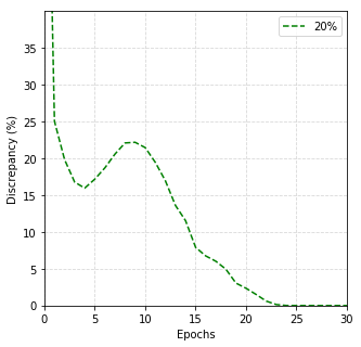
(a) $D_{t}$ curve

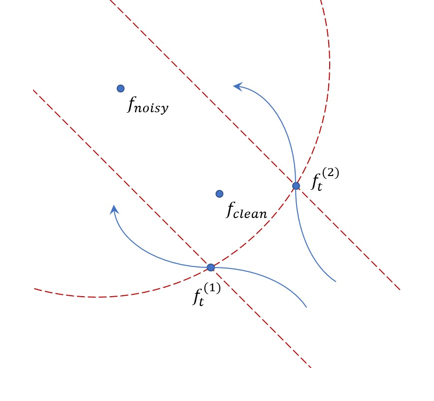
(b) Dynamics in function space

Figure 1: Double descent of discrepancy

This phenomenon is counter intuitive! What it has implied is that even though identically-trained networks are approaching the same target function $f_{noisy}$, at some point, they diverge from each other. Figure 1(b) illustrate the dynamics of $f^{(1)},f^{(2)}$ in function space. At time step $t$, their training errors still decrease, but the discrepancy between them increases. This strange dynamic means there exist fundamental non-linearity in DNNs’ training process.

Remark. While the "double descent of discrepancy" phenomenon share a similar name with the "double descent" phenomenon, the two are distinct and unrelated. The $\text{D}^{3}$ phenomenon characterizes the discrepancy between two identically-trained networks on the training dataset, where the "double descent" phenomenon focuses on the single network’s generalization ability.

1.3 Our contributions

Our main contributions in this work are:

1. We discover and report the "double descent of discrepancy" phenomenon in neural network training. We find that, if there exists a certain level of noise in the training dataset, the discrepancy between identically-trained networks will increase at some point in the training process. This counter-intuitive phenomenon provides new insights into the complex behaviors of DNNs.

2. In Section 2, we conduct extensive experiments to demonstrate the prevalence of the $\text{D}^{3}$ phenomenon. We show that it occurs across different tasks (e.g. classification, implicit neural representation), datasets (e.g. CIFAR-10, Mini-ImageNet), and network architectures (e.g. VGG, ResNet, DenseNet). These experiments empirically show that this phenomenon appears commonly in DNN training processes.

3. In Section 3, we propose an early stopping criterion based on the $\text{D}^{3}$ phenomenon. We evaluate its performance on image denoising tasks and compare with another existing early stopping criterion. We demonstrate that our criterion outperforms the other. Furthermore, we prove a theorem that describes the relationship between the early stopping time and the increase in discrepancy.

4. In Section 4, we develop a new method for data quality assessment. We empirically show that the $\text{D}^{3}$ phenomenon is related with the data quality of the training dataset, with the maximum degree of discrepancy linearly related to the noise level. Based on this insight, we propose that the degree of discrepancy can serve as an effective proxy for data quality.

In summary, this work practices the phenomenon-driven approach we introduced before. We observe a prevalent yet counter-intuitive phenomenon in DNN training. Through extensive experiments, we demonstrate that this phenomenon is widespread across different experimental settings. Based on insights gained from this phenomenon, we propose an early stopping criterion and a data quality assessment method. We believe that discovering and understanding more phenomena like this can provide fundamental insights into complex DNN models and guide the development of deep learning to a more scientific level.

2 Double descent of discrepancy

In this section, we demonstrate that the $\text{D}^{3}$ phenomenon is widespread across various tasks, datasets, and network architectures. As training progresses, $D_{t}$ first decreases, then increases, and finally decreases to zero. We also provide a brief discussion of this phenomenon at the end of the section.

2.1 Classification

Experimental setup. For classification tasks, we run experiments on CIFAR-10, CIFAR-100, and Mini-ImageNet [12]. The network architectures include Visual Geometry Group (VGG) [13], Residual Networks (ResNet) [14], Densely Connected Convolutional Networks (DenseNet) [15] and some more updated architectures such as Vision Transformer [16, 17, 18]. For each dataset, we corrupt a fraction of labels by replacing them with random labels to introduce noise. Networks are trained on these corrupted datasets with momentum SGD. The level of corruption and training hyper-parameters can also be modified. See Appendix B.1 for setting details.

Since in classification the cross-entropy loss function $l(\cdot,\cdot)$ is not symmetric, we defined the discrepancy function as $d(y_{1},y_{2})=\|y_{1}-y_{2}\|_{\infty}=\mathbb{I}_{{y_{1}=y_{2}}}$.

During training, identically-trained networks undergo exactly the same procedure. For instance, they process batches in the same order. This allows us to calculate their discrepancy by using networks’ forward propagation results, thus minimizing the computational cost.

(a) CIFAR-10, VGG

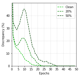
(b) CIFAR-10, ResNet

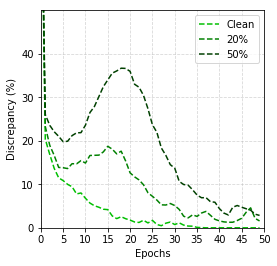
(c) CIFAR-10, DenseNet

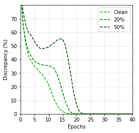
(d) Mini-ImageNet, VGG

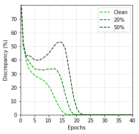
(e) Mini-ImageNet, ResNet

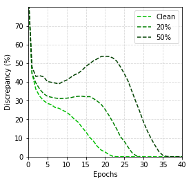
(f) Mini-ImageNet, DenseNet

Figure 2: $D_{t}$ curves, classification.

Result. Figure 2 shows some examples of $D_{t}$ curves. Due to space limitation, here we only present results for the CIFAR-10 and Mini-ImageNet datasets, and the VGG, ResNet, and DenseNet network architectures. Each dataset is corrupted by 0% (clean), 20%, and 50%. More results are provided in Appendix B.1.

In all plots, when a certain portion of the labels are corrupted, the $\text{D}^{3}$ phenomenon emerges. While the shapes of the $D_{t}$ curves differ, they exhibit the same pattern. These results demonstrate that the $\text{D}^{3}$ phenomenon is data- and model-agnostic. It can also be observed from the plots that the $\text{D}^{3}$ phenomenon becomes more pronounced as the corruption rate in the dataset increases.

2.2 Implicit neural representation

Experimental setup. For implicit neural representation tasks, we use neural networks to represent images in the classical 9-image dataset [19]. The network architectures include fully connected neural networks with periodic activations (SIREN) [20] and deep image prior (DIP) [21]. Here, we treat DIP as a special kind of neural representation architecture. We add different levels of Gaussian noise on these images to create their noisy versions. The networks are trained on noisy images using Adam. The corruption level and hyper-parameters in training are also adjustable. For more details, see Appendix B.2.

The loss function used here is the $l$-2 loss, so we simply take $d(y_{1},y_{2})=l(y_{1},y_{2})=\|y_{1}-y_{2}\|^{2}_{2}$.

Results. Figure 3 shows some examples of $D_{t}$ curves. For the same reason, here we only present SIREN and DIP trained on the "House" image corrupted by Gaussian noise with zero mean and standard deviations $\sigma=0,25,50$. More results are provided in Appendix B.2.

We can see that in neural representation tasks the $\text{D}^{3}$ phenomenon also emerges, demonstrating that it is task-agnostic. Furthermore, even though SIREN and DIP varies dramatically in network architecture, the patterns of their $D_{t}$ curves are quite similar.

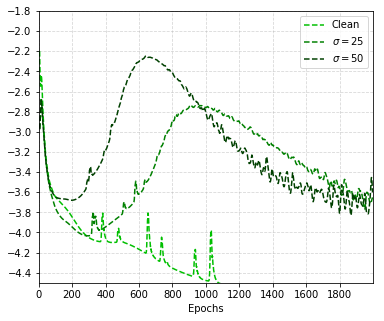
(a) SIREN

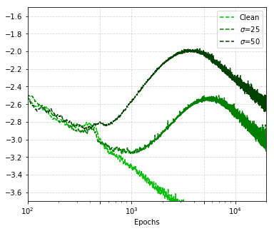
(b) DIP

Figure 3: $\log_{10}{D_{t}}$ curves, implicit neural representation.

2.3 Other tasks

We have also conducted experiments on regression tasks and graph-related tasks. Due to space limitation, we provide their results in Appendix B.3 and B.4. In all these tasks, the $\text{D}^{3}$ phenomenon emerges, further demonstrating that it is task-agnostic.

2.4 Brief discussion

Based on these experimental results, we are confident to say that the double descent of discrepancy is a prevalent phenomenon in DNN training. However, it does not appear in linear feature models or any model that exhibits linear properties during training, such as the infinite wide network discussed in neural tangent kernel (NTK) [22]. This is rigorously proved in Appendix A. This difference may help us understand how DNNs differ from conventional parametric models. Explaining this phenomenon is challenging, as it involves fundamentally non-linear behavior of DNNs during their training process. We have partly explained it in Section 3, but our understanding remains elementary.

3 Early stopping criterion

In machine learning, early stopping is a common technique used to avoid overfitting. By stopping the training process at an appropriate time, models can achieve good generalization performance even when trained on very noisy dataset [23].

The key factor in early stopping is the stopping criterion, which determines when to stop training. The most common criteria are validation-based, which involve monitoring the model’s generalization performance on a validation set and stopping training when the validation error starts increasing. However, as pointed out in [24, 25], validation-based criteria have several drawbacks: they bring extra computational costs, reduce the number of training samples, and have high variability in performance. In some cases, it may not even be possible to construct a validation set. These drawbacks have motivated researchers to develop criteria without validation sets [24, 26, 27].

In this section, we demonstrate how the $\text{D}^{3}$ phenomenon can be used to construct an early stopping criterion. We evaluate its performance on image denoising tasks and compare it with another pre-existing criterion. Furthermore, we prove a theorem that formally establishes the relationship between early stopping time and the increase in discrepancy.

3.1 Our criterion

The optimal stopping time for the $j$-th network is defined as $\tau^{(j)}=arg\min_{t}d_{N}(f^{(j)}_{t},f_{clean})$.

Our criterion stops training when $D_{t}$ begins to increase. More precisely, the stopping time $\tau_{\alpha}$ given by our criterion is:

$$\tau_{\alpha}=\inf\left\{t\ |\ \frac{d}{dt}D_{t}>\alpha\right\},$$ (2)

where $\alpha$ is a hyper-parameter.

Since the time step $t$ is discrete, $\frac{d}{dt}D_{t}$ is approximated by its discrete difference $(\tilde{D}_{t+1}-\tilde{D}_{t})/\Delta t$. To minimize fluctuations from randomness, here we use the moving average $\tilde{D}_{t}=\frac{1}{w}\sum_{i=0}^{w-1}D_{t+i}$ instead of $D_{t}$, where $w$ is the window size.

Simply setting $\alpha=0$ would give a fairly good criterion. However, with more information about the model and dataset, one could choose a better $\alpha$ that improves performance. In Section 3.3, we explain how to choose a better $\alpha$.

3.2 Image denoising

For image denoising tasks, $f_{clean}$ is the clean image we want to recover, and $f_{noisy}$ is the noisy image. Here, $x$ represents the pixel position, and $f(x)$ represents the RGB value of the corresponding position. If we stop the training at a proper time $\tau$, $f_{\tau}$ would be close to $f_{clean}$ thus filter out the noise.

Experimental setup. We use DIP as our DNN model and evaluate the performance of our criterion on the 9-image dataset. We compare our criterion with ES-WMV[28], a stopping criterion specifically designed for DIP. We adopt their experimental settings and use the PSNR gap (the difference in PSNR values between $f^{(j)}_{\tau}$ and $f^{(j)}_{\tau^{(j)}}$) to measure the criterion performance.

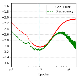
(a) House

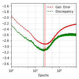
(b) Peppers

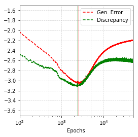
(c) F16

Figure 4: Different stopping times. Red: optimal. Green: our criterion.

Table 1: PSNR gaps, Gaussian noise, $\sigma=25$

	House	Pep.	Lena	Bab.	F16	K01	K02	K03	K12
ES-WMV	1.42	1.02	0.39	3.87	0.72	0.40	1.62	1.39	1.63
Ours	0.30	0.25	0.31	4.26	0.30	0.76	0.76	0.93	0.56

Results. Table 1 has listed the performances of ES-WMV and our criterion. Here, the noises are Gaussian noises with zero mean and standard deviation $\sigma=25$. As shown in the table, our criterion outperform ES-WMV in seven out of nine images, is not as good in one, and both perform poorly in one. Additionally, we present some examples of stopping time $\tau$ given by our criterion compare to the optimal stopping time $\tau^{(j)}$ in Figure 4. As shown in the figure, they are very close to each other. More results are provided in Appendix C. To ensure fairness, here we set $\alpha=0$ in our criterion.

It is worth pointing out that our criterion is not task-specific but rather a general criterion, yet here it works better than a specifically designed criterion. Furthermore, from its definition one can see that it is an adaptive criterion, which means it is robust to changes in network architecture or learning algorithms. We expect these performances do not represent the limit of our criterion and that better results can be achieved through hyperparameter tuning.

3.3 Mathematical explanation

In this subsection, we establish the connection between the optimal stopping time and the increase of discrepancy. For simplicity, we assume that $l(y_{1},y_{2})=d(y_{1},y_{2})=\|y_{1}-y_{2}\|^{2}$ and approximate the gradient descent by gradient flow:

$$\frac{d}{dt}\theta=-\nabla_{\theta}d_{N}(f_{t},f_{noisy}),$$

Given neural network $f(x;\theta)$, we define neural kernel as $K=\nabla_{\theta}f\otimes\nabla_{\theta}f$ and define $\langle g,h\rangle_{K}$ as the inner product induced by $K$:

$$\langle g,h\rangle_{K}=\frac{1}{N^{2}}\sum_{x_{i},x_{j}^{{}^{\prime}}\in S_{N,\mathcal{X}}}g^{T}(x_{i})K(x_{i},x_{j}^{{}^{\prime}})h(x_{j}^{{}^{\prime}})$$

Notice for $t$ near the optimal stopping time $\tau^{(j)}$, $t>\tau^{(j)}$ is equivalent with $\frac{d}{dt}d_{N}(f_{t}^{(j)},f_{clean})>0$. Meanwhile, $\frac{d}{dt}D_{t}>0$ equals with $\frac{d}{dt}d_{N}(f_{t}^{(1)},f_{t}^{(2)})>0$. The theorem bellow states the relationship between these two inequalities. It shows that under certain condition, they are almost equivalent.

Theorem. If at time step $t$, $f^{(j)}_{t}$ satisfies that $\forall j,$

$$|\langle f_{t}^{(-j)}-f_{clean},f_{t}^{(j)}-f_{clean}\rangle_{K_{t}^{(j)}}|<\delta/2,$$ (3)

$$|\langle f_{t}^{(-j)}-f_{clean},f_{noisy}-f_{clean}\rangle_{K_{t}^{(j)}}|<\epsilon/2.$$ (4)

then we have the following two results:

1. $\frac{d}{dt}d_{N}(f_{t}^{(1)},f_{t}^{(2)})>\delta+\epsilon$ implies $\exists j,\ \frac{d}{dt}d_{N}(f_{t}^{(j)},f_{clean})>0;$

2. $\forall j,\ \frac{d}{dt}d_{N}(f_{t}^{(j)},f_{clean})>0$ implies $\frac{d}{dt}d_{N}(f_{t}^{(1)},f_{t}^{(2)})>-(\delta+\epsilon)$

Here, $K_{t}^{(j)}$ represents the neural kernel of $f_{t}^{(j)}$.

Proof. See Appendix C for the proof.

For any $\delta$ and $\epsilon$, there exists a set of time steps $T_{\delta,\epsilon}=\{t\ |\ f_{t}^{(j)}\text{satisfies the condition}\}$. At these time steps, our theorem shows that these two inequalities are equivalent with a difference of $\delta+\epsilon$. The smaller the sum $\delta+\epsilon$, the tighter this equivalence. However, note that smaller $\delta$ and $\epsilon$ values lead to a condition that is harder to satisfy, thus lead to a smaller set $T_{\delta,\epsilon}$.

We argue that conditions $(\ref{cond1})$ and $(\ref{cond2})$ of the theorem are relatively mild. We demonstrate this by showing that small $\delta$ and $\epsilon$ are sufficient for $T_{\delta,\epsilon}$ to be non-empty.

Condition $(\ref{cond1})$ is automatically satisfied if $\|f_{t}^{(k)}-f_{clean}\|^{2}\lesssim{\delta/\|{K_{t}^{(j)}}\|},\ \forall j,k$. So the smallest $\delta$ for $T_{\delta,\epsilon}$ to be non-empty is $\delta^{*}\sim\|K_{\tau^{(j)}}\|\|f_{\tau^{(j)}}-f_{clean}\|^{2}$. The better the generalization performance of the early stopped model $f_{\tau^{(j)}}$, the smaller $\delta^{*}$ is. Estimation of generalization error $\|f_{\tau^{(j)}}-f_{clean}\|$ requires considering the dataset, network architecture, and training algorithm, which is far beyond the scope of this work. However, the effectiveness of early stopping method gives us confidence that a relatively small $\delta^{*}$ can be achieved.

Condition $(\ref{cond2})$ can be justified by Fourier analysis. Notice that $f_{noisy}-f_{clean}$ is pure noise, which means it primarily comprises high frequency components, while $K_{t}(f_{t}-f_{clean})$ primarily comprises low frequency components. This means that they are almost orthogonal in the function space and their inner product can be controlled by a small constant $\epsilon^{*}$.

These analyses show that $\delta^{*}+\epsilon^{*}$ is relatively small, which means the conditions of this theorem are relatively mild.

One may note that the early stopping times given by our criterion are always ahead of the optimal stopping times. This can be avoided by choosing some $\alpha>0$ in the stopping criterion. In fact, to achieve better performance, one could take $\alpha\sim\delta^{*}+\epsilon^{*}$. More discussions on setting $\alpha$ are provided in Appendix C.

4 Data quality assessment

As machine learning models rely heavily on large amounts of data to train, the quality of the datasets used is crucial. However, sometimes high-quality datasets can be expensive and difficult to obtain. As a result, cheaper or more accessible datasets are often used as an alternative [29, 30]. However, these datasets may lack guarantees on data quality and integrity, which can negatively impact model performance. It is therefore important to have methods to assess the quality of datasets in order to understand potential issues and limitations. By vetting the quality of datasets, we can produce more reliable machine learning models.

Data quality assessment include many evaluating aspects. Here, we focus on the accuracy of labels. As we have mentioned in section 2, the greater the noise level, the more pronounced the $\text{D}^{3}$ phenomenon. In this section, we quantify this relationship and show how it can be used for data quality assessment. We first clarify some definitions, then establish our method and use the CIFAR-10 dataset as an example to demonstrate it.

4.1 Definitions

We define the noise level of the training dataset as $E=d_{N}(f_{noisy},f_{clean})$. For example, in classification tasks, $E$ represents the label corruption rate.

For the $\text{D}^{3}$ phenomenon, we define the maximum discrepancy between two networks as:

$$D^{*}=\max_{t>\tau_{0}}D_{t},$$ (5)

where $\tau_{0}$ is the time step where $D_{t}$ begins to increase, as defined in (2). Intuitively, $D^{*}$ quantifies the height of the peak in a $D_{t}$ curve.

4.2 Our method

We demonstrate our method using the CIFAR-10 dataset and the ResNet model. The experimental setups are basically the same as in Section 2.1. Here we corrupt CIFAR-10 by 10%, …,90%, 100% (pure noise) and use it as our noisy datasets. We compute the values of $D^{*}$ on these datasets and plot its relationship with noise level $E$ in Figure 5. As shown in the plots, $D^{*}$ vs $E$ can be well approximated by linear functions, with $R^{2}=0.991523$. This indicates a strong correlation between the maximum discrepancy $D^{*}$ and the noise level $E$.

Such an accurate fit means we can use it to evaluate the noise level of other similar datasets. For example, if we want to evaluate a new noisy dataset that is similar to CIFAR-10, then we could compute $D^{*}$ and use Figure 5 to get a rough estimation of noise level $E$. However, we have to point out that differences in the dataset, such as size or sample distribution, may affect these linear relationships and make our estimation inaccurate. Thus, only for datasets that are very similar with the original dataset, such as a new dataset generate from the same distribution, will this estimation approach be accurate.

The underlying cause of this linear relationship remains a mystery. Our hypothesis is that, for time steps $\tau_{0}<t<\tau_{0}+\Delta t$ where networks begin overfitting to noise, different networks fit different components of the pure noise $f_{noisy}-f_{clean}$ that are nearly orthogonal. Since identically-trained networks are similar to one another near $\tau_{0}$, new orthogonal increments would cause $D_{t}$ to increase. Therefore, the maximum discrepancy $D^{*}$ is linearly related to the maximum length of the orthogonal components of pure noise $f_{noisy}-f_{clean}$, which is linearly related to the noise level $E$. This explanation is rough and lacks mathematical rigor. We aim to prove it mathematically in future works.

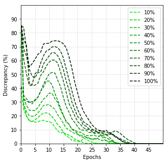
(a) $D_{t}$ curves

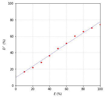
(b) $E$ vs $D^{*}$

Figure 5: Noise level vs max discrepancy. CIFAR-10, ResNet.

5 Conclusion

In this paper, we discovered a counter-intuitive phenomenon that the discrepancy of identically-trained networks does not decrease monotonically, but exhibits the $\text{D}^{3}$ phenomenon. This phenomenon differentiates simple linear models and complex DNNs. We conducted extensive experiments to demonstrate that it is task-, data-, and model-agnostic. Leveraging insights from this phenomenon, we proposed a new early stopping criterion and a new data quality assessment method.

While this paper reveals new insights into complex DNN behaviors, our understanding remains limited. There are many aspects of this phenomenon left to be discovered and explained, such as identifying the necessary conditions for this phenomenon to emerge. Additionally, many of the findings presented in this paper lack rigorous mathematical proofs and formal analyses. These are all possible directions for future works.

In summary, through observing and analyzing the $\text{D}^{3}$ phenomenon, we gain new insights into DNNs that were previously not well understood. This work showcases the power of a phenomenon-driven approach in facilitating progress in deep learning theory and practice. We believe discovering and understanding more such phenomena is crucial for developing a systematic and principled understanding of DNNs.

Appendix

Appendix A Results for linear models

In this section, we strictly state and proof that the discrepancy between identically-trained linear feature models decreases monotonically. Thus, no matter how noisy the training set is, it does not exhibit the $\text{D}^{3}$ phenomenon.

By the term "linear feature models", we refer to models with the form below:

$$f(x;\theta_{t})=\sum_{i=1}^{P}(\theta_{t})_{i}\phi_{i}(x)$$

where $\phi_{i}:\mathcal{X}\to\mathcal{Y}$ are the features.

Like what we did in Section 3, here we assume that $d(y_{1},y_{2})=l(y_{1},y_{2})=\|y_{1}-y_{2}\|^{2}$ and approximate the gradient descent by the gradient flow:

$$\frac{d}{dt}\theta_{t}=-\nabla_{\theta}d_{N}(f_{t},f_{noisy})$$

Then, we have the proposition below.

Proposition. For identically-trained linear feature models $f_{t}^{(1)}$ and $f_{t}^{(2)}$, their discrepancy on the training dataset $D_{t}=d_{N}(f_{t}^{(1)},f_{t}^{(2)})$ decreases monotonically, i.e.

$$\frac{d}{dt}D_{t}\leqslant 0,\ \forall t.$$

Proof. For linear feature models, gradient flow can be specified as:

$$\frac{d}{dt}(\theta_{t})_{i}=-2\langle f_{t}-f_{noisy},\phi_{i}\rangle,$$

where $\langle\cdot,\cdot\rangle$ represents the inner product on $S_{N,\mathcal{X}}$:

$$\langle f,g\rangle=\frac{1}{N}\sum_{i=1}^{N}f(x_{i})^{T}g(x_{i}).$$

This gives:

$$\frac{d}{dt}f^{(j)}_{t}=\sum_{i=1}^{P}\frac{d}{dt}(\theta^{(j)}_{t})_{i}\phi_{i}=-2\sum_{i=1}^{P}\langle f^{(j)}_{t}-f_{noisy},\phi_{i}\rangle\phi_{i}.$$

Notice that $df^{(j)}_{t}/dt$ depend linearly on $f^{(j)}_{t}$, which means:

$$\frac{d}{dt}(f^{(1)}_{t}-f^{(2)}_{t})=-2\sum_{i=1}^{P}\langle f^{(1)}_{t}-f^{(2)}_{t},\phi_{i}\rangle\phi_{i}.$$

Thus gives the result of the proposition:

$$\frac{d}{dt}D_{t}=2\langle f^{(1)}_{t}-f^{(2)}_{t},\frac{d}{dt}(f^{(1)}_{t}-f^{(2)}_{t})\rangle=-4\sum_{i=1}^{P}\langle f^{(1)}_{t}-f^{(2)}_{t},\phi_{i}\rangle^{2}\leqslant 0.$$

$\hfill{\square}$

Remark. It is worth noting that for any model that exhibits a linear training dynamic, the $l$-2 discrepancy between identically-trained networks decreases monotonically. By "linear training dynamic", we refer to dynamic with the form of:

$$\frac{d}{dt}f=-G(f_{t}-f{noisy})$$

where $G$ is a semi-definite linear operator.

This means that our proposition can be generated to include more network architectures, includes the infinite wide neural networks studied in NTK. However, as demonstrated in our work, complicated neural networks do not behave like this.

Appendix B Experimental settings and results

B.1 Classification

For each classification dataset, we corrupt a fraction of labels by replacing them with randomly generated labels to introduce noise. The random labels are uniformly distributed across all possible labels, including the correct label. This means that even when all labels are corrupted, some labels will remain correct due to randomness. For example, in a 100% corrupted CIFAR-10 dataset, around 10% of the labels will remain correct.

The network architectures we used include:

1. VGG-16 in [13];

2. ResNet-18 in [14];

3. DenseNet-121 in [15];

4. Deep layer aggregation (DLA-34) in [17];

5. Squeeze-and-excitation network (SENet-18) in [18];

6. Vision Transformer (ViT-B) in [16].

All networks are trained with SGD with a momentum of 0.9 and weight decay of 1E-4. Learning rate is 0.01 without decay (since we want the networks to overfit). We perform data augmentation and use a minibatch size of 100 for CIFAR-10 and CIFAR-100, and a size of 50 for Mini-ImageNet. As for noise level, CIFAR-10 is corrupted by 0%, 20%, and 50%, where CIFAR-100 and Mini-ImageNet are corrupted by 0%, 30% and 50%.

It should be pointed out that in order to maintain a consistent experimental setting, many of these networks are not trained to state-of-the-art accuracy. However, the $\text{D}^{3}$ phenomenon is not sensitive to specific training methods. Therefore, differences in training method are not a key factor for this phenomenon.

The results are presented in Figure 6, 7, and 8. In all plots, the $\text{D}^{3}$ phenomenon emerges.

(a) VGG

(b) ResNet

(c) DenseNet

(d) DLA

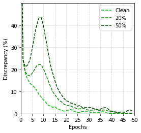
(e) SENet

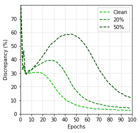
(f) ViT

Figure 6: $D_{t}$ curves, classification, CIFAR-10

(a) VGG

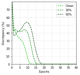
(b) ResNet

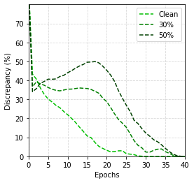
(c) DenseNet

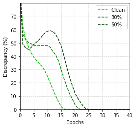
(d) DLA

(e) SENet

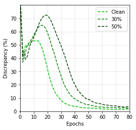
(f) ViT

Figure 7: $D_{t}$ curves, classification, CIFAR-100

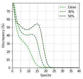
(a) VGG

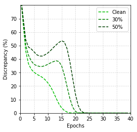
(b) ResNet

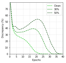
(c) DenseNet

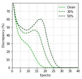
(d) DLA

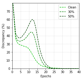
(e) SENet

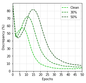
(f) ViT

Figure 8: $D_{t}$ curves, classification, Mini-ImageNet

B.2 Implicit neural representation

For each image in image-9, we add Gaussian noises with zero mean and standard deviation $\sigma=0,25,50$ to create a noisy image.

For SIREN, we use the model given in [20]’s demo, which has 3 hidden layers and 256 hidden features. For DIP, we use the model given in [21]’s demo. DIP represents images with a generative deep network, i.e. $f_{\theta}=G_{\theta}(z)$, where $z$ is an input noise. Here, we use the same $z$ between identically-trained networks. Also, following the original setup, we perturb $z$ during the training process. In Section 2.2, Section 3, and Appendix C, at each step we perturb $z$ with additive normal noise with zero mean and standard deviation $\sigma_{p}=0.05$, which follows the setting of [21]. Here, in order to better illustrate the $\text{D}^{3}$ phenomenon, we took $\sigma_{p}=0.02$.

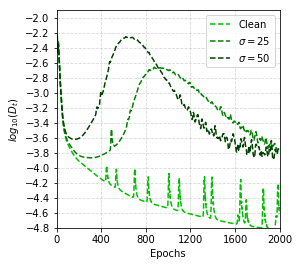
(a) Peppers

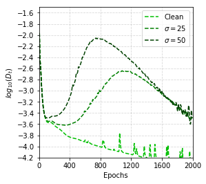
(b) F16

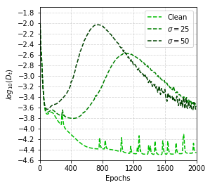
(c) Kodak12

Figure 9: $D_{t}$ curves, implicit neural representation, SIREN

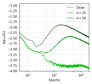
(a) Peppers

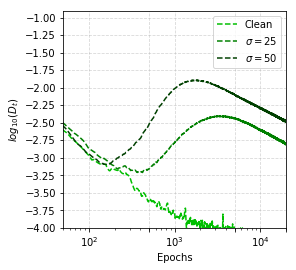
(b) F16

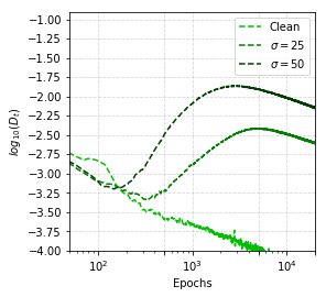
(c) Kodak12

Figure 10: $D_{t}$ curves, implicit neural representation, DIP

SIRENs and DIPs are trained with Adam. For SIREN, we use PyTorch’s default Adam hyperparameters. For DIP, we take a learning rate of 0.01 while keeping other hyperparameters unchanged.

Results for image "Peppers", "F16", and "Kodak12" are presented in Figure 9 and 10. In all plots, the $\text{D}^{3}$ phenomenon emerges.

B.3 Regression

For regression tasks, we manually construct some analytical functions to serve as $f_{clean}$. To generate the training dataset, we sample $x_{i}$ uniformly in a bound set $\Omega\subset\mathcal{X}$, and calculate $y_{i}=f_{clean}(x_{i})+\epsilon_{i}$, where $\epsilon_{i}\sim_{i.i.d.}\mathcal{N}(0,\sigma)$. More specifically, here we take $f_{clean}$ as the 1-dimensional sigmoid function $f_{clean}(x)=2/(1-e^{-x})-1$ and generate 100 samples $(x_{i},y_{i})$ where $x_{i}\sim\mathcal{U}[-2,2]$.

The network architecture we chose for this task is a 4-layer deep, 512-unit wide fully connected neural network with ReLU activation function. We train these networks with momentum GD. The hyperparameters are: learning rate 1E-3, momentum 0.9, and weight decay 1E-4.

The results for $\sigma=0,0.5,1$ are presented in Figure 11(a). Again, the $\text{D}^{3}$ phenomenon emerges. It should be noted that the $\text{D}^{3}$ phenomenon does not occur every time under this setting. Our understanding is that the 4-layer FNN we used here is simple and does not have as many parameters as the networks used in the previous two tasks.

B.4 Graph related tasks

We have also conducted experiments on the classification tasks of nodes in a graph. We use the citation network dataset Cora [31] as our basic dataset, and corrupt its labels by 0%, 30%, and 50%. The network architecture we use is a 4-layer deep, 256-unit wide graph convolution network (GCN) given in [32]. We train these networks with momentum GD. The hyperparameters are: learning rate 0.01, momentum 0.9, and weight decay 1E-4.

The results are presented in Figure 11(b). Again, the $\text{D}^{3}$ phenomenon emerges.

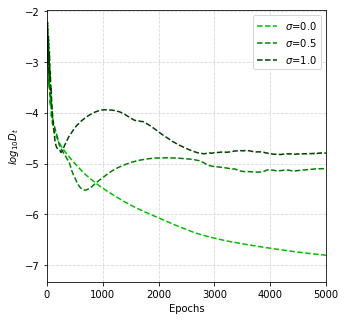
(a) Toy regression

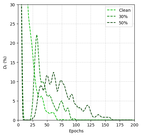
(b) Classification on graph

Figure 11: $D_{t}$ curves. Other tasks.

Appendix C Early stopping criterion

C.1 Image denoising

Here, we we adopt the same experimental setup as in Appendix B.2.

The strict definition of PSNR gap in Section 3 is:

$$\Delta\text{PSNR}=\text{PSNR}(f_{\tau^{(1)}};f_{clean})-\text{PSNR}(f_{\tau_{\alpha}};f_{clean})$$

where $\text{PSNR}(f;f_{clean})$ is the peak signal-to-noise ratio of output $f$.

We present more examples of early stopping times $\tau_{0}$ given by our criterion in Figure 12. As one can see, the problem with our criterion is that it always stops the training too early. As we discussed in the paper, this problem can be avoided by choosing an appropriate hyperparameter $\alpha$.

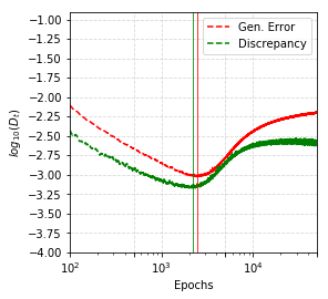
(a) Lena

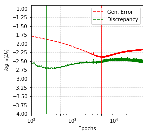
(b) Baboon

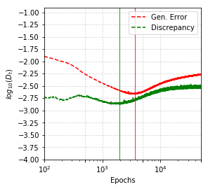
(c) Kodak01

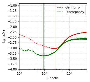
(d) Kodak02

(e) Kodak03

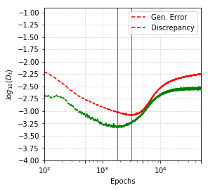
(f) Kodak12

Figure 12: Different stopping times. Red: optimal. Green: our criterion.

C.2 Theorem and proof

With the definitions given in Section 3, we have the theorem below.

Theorem. If at time step $t$, $f^{(j)}_{t}$ satisfies that $\forall j,$

$$|\langle f_{t}^{(-j)}-f_{clean},f_{t}^{(j)}-f_{clean}\rangle_{K_{t}^{(j)}}|<\delta/2,$$

$$|\langle f_{t}^{(-j)}-f_{clean},f_{noisy}-f_{clean}\rangle_{K_{t}^{(j)}}|<\epsilon/2.$$

then we have the following two results:

1. $\frac{d}{dt}d_{N}(f_{t}^{(1)},f_{t}^{(2)})>\delta+\epsilon$ implies $\exists j,\ \frac{d}{dt}d_{N}(f_{t}^{(j)},f_{clean})>0;$

2. $\forall j,\ \frac{d}{dt}d_{N}(f_{t}^{(j)},f_{clean})>0$ implies $\frac{d}{dt}d_{N}(f_{t}^{(1)},f_{t}^{(2)})>-(\delta+\epsilon)$

Here, $K_{t}^{(j)}$ represents the neural kernel of $f_{t}^{(j)}$.

Proof. Here, we only prove result 2 since the proof for these two results are quite similar.

Take the full differential of $\frac{d}{dt}d_{N}(f_{t}^{(1)},f_{t}^{(2)})$:

$$\frac{d}{dt}d_{N}(f_{t}^{(1)},f_{t}^{(2)})= \nabla_{\theta^{(1)}}d_{N}(f_{t}^{(1)},f_{t}^{(2)})\frac{d}{dt}\theta^{(1)}+\nabla_{\theta^{(2)}}d_{N}(f_{t}^{(1)},f_{t}^{(2)})\frac{d}{dt}\theta^{(2)}$$

$$= -\left(\nabla_{\theta^{(1)}}d_{N}(f_{t}^{(1)},f_{t}^{(2)})\right)^{T}\left(\nabla_{\theta^{(1)}}d_{N}(f_{t}^{(1)},f_{noisy})\right)$$

$$-\left(\nabla_{\theta^{(2)}}d_{N}(f_{t}^{(1)},f_{t}^{(2)})\right)^{T}\left(\nabla_{\theta^{(2)}}d_{N}(f_{t}^{(2)},f_{noisy})\right)$$

$$= -\langle f_{t}^{(1)}-f_{t}^{(2)},\nabla_{\theta^{(1)}}f_{t}^{(1)}\rangle^{T}\langle f_{t}^{(1)}-f_{noisy},\nabla_{\theta^{(1)}}f_{t}^{(1)}\rangle$$

$$-\langle f_{t}^{(2)}-f_{t}^{(1)},\nabla_{\theta^{(2)}}f_{t}^{(2)}\rangle^{T}\langle f_{t}^{(2)}-f_{noisy},\nabla_{\theta^{(2)}}f_{t}^{(2)}\rangle$$

$$= -\langle f_{t}^{(1)}-f_{t}^{(2)},f_{t}^{(1)}-f_{noisy}\rangle_{K_{t}^{(1)}}-\langle f_{t}^{(2)}-f_{t}^{(1)},f_{t}^{(2)}-f_{noisy}\rangle_{K_{t}^{(2)}}$$

Under theorem’s condition,

$$\langle f_{t}^{(1)}-f_{t}^{(2)},f_{t}^{(1)}-f_{noisy}\rangle_{K_{t}^{(1)}}=\ \langle f_{t}^{(1)}-f_{clean},f_{t}^{(1)}-f_{noisy}\rangle_{K_{t}^{(1)}}-\langle f_{t}^{(2)}-f_{clean},f_{t}^{(1)}-f_{noisy}\rangle_{K_{t}^{(1)}}$$

$$=\ \langle f_{t}^{(1)}-f_{clean},f_{t}^{(1)}-f_{noisy}\rangle_{K_{t}^{(1)}}$$

$$-\left(\langle f_{t}^{(2)}-f_{clean},f_{t}^{(1)}-f_{clean}\rangle_{K_{t}^{(1)}}-\langle f_{t}^{(2)}-f_{clean},f_{noisy}-f_{clean}\rangle_{K_{t}^{(1)}}\right)$$

$$<\ \langle f_{t}^{(1)}-f_{clean},f_{t}^{(1)}-f_{noisy}\rangle_{K_{t}^{(1)}}+(\delta+\epsilon)/2$$

Similarly, $\langle f_{t}^{(2)}-f_{t}^{(1)},f_{t}^{(2)}-f_{noisy}\rangle_{K_{t}^{(2)}}<\ \langle f_{t}^{(2)}-f_{clean},f_{t}^{(2)}-f_{noisy}\rangle_{K_{t}^{(2)}}+(\delta+\epsilon)/2$.

This leads to:

$$\frac{d}{dt}d_{N}(f_{t}^{(1)},f_{t}^{(2)})= -\langle f_{t}^{(1)}-f_{t}^{(2)},f_{t}^{(1)}-f_{noisy}\rangle_{K_{t}^{(1)}}-\langle f_{t}^{(2)}-f_{t}^{(1)},f_{t}^{(2)}-f_{noisy}\rangle_{K_{t}^{(2)}}$$

$$> -\langle f_{t}^{(1)}-f_{clean},f_{t}^{(1)}-f_{noisy}\rangle_{K_{t}^{(1)}}-\langle f_{t}^{(2)}-f_{clean},f_{t}^{(2)}-f_{noisy}\rangle_{K_{t}^{(2)}}-(\delta+\epsilon)$$

$$= \ \frac{d}{dt}d_{N}(f_{t}^{(1)},f_{clean})+\frac{d}{dt}d_{N}(f_{t}^{(2)},f_{clean})-(\delta+\epsilon)$$

Thus, $\forall j,\ \frac{d}{dt}d_{N}(f_{t}^{(j)},f_{clean})>0$ implies $\frac{d}{dt}d_{N}(f_{t}^{(1)},f_{t}^{(2)})>-(\delta+\epsilon).$

It is easy to see that result 1 can be proved similarly. $\hfill{\square}$

We have empirically observed that in most circumstances, for $t$ near ${\tau_{0}}$:

$$\frac{d}{dt}d_{N}(f_{t}^{(1)},f_{t}^{(2)})>\frac{d}{dt}d_{N}(f_{t}^{(1)},f_{clean})+\frac{d}{dt}d_{N}(f_{t}^{(2)},f_{clean}).$$

This means that when the discrepancy began to increase, the networks could still be heading towards $f_{clean}$, which means $\tau_{0}$ is always ahead of $\tau^{(j)}$, i.e. $\tau_{0}<\tau^{(j)}$.

The reason for this is still unclear, but we believe an important factor is that:

$$\langle f_{\tau_{0}}^{(-j)}-f_{clean},f_{\tau_{0}}^{(j)}-f_{clean}\rangle_{K_{\tau_{0}}^{(j)}}>0$$

This inequality means there exist some components of $f_{clean}$ that are difficult for all identically-trained networks to learn. Take this inequality as an assumption, it is easy to see that the condition in Result 1 can be weakened to $\frac{d}{dt}d_{N}(f_{t}^{(1)},f_{t}^{(2)})>\epsilon$.

This is also why we suggest in Section 3 that one should choose $\alpha>0$ instead of $\alpha<0$.

References

- [1] Mikhail Belkin, Daniel J. Hsu, Siyuan Ma, and Soumik Mandal. Reconciling modern machine-learning practice and the classical bias–variance trade-off. Proceedings of the National Academy of Sciences, 116:15849 – 15854, 2018.
- [2] Preetum Nakkiran, Gal Kaplun, Yamini Bansal, Tristan Yang, Boaz Barak, and Ilya Sutskever. Deep double descent: where bigger models and more data hurt. Journal of Statistical Mechanics: Theory and Experiment, 2021, 2019.
- [3] Reinhard Heckel and Fatih Yilmaz. Early stopping in deep networks: Double descent and how to eliminate it. ArXiv, abs/2007.10099, 2020.
- [4] Zitong Yang, Yaodong Yu, Chong You, Jacob Steinhardt, and Yi Ma. Rethinking bias-variance trade-off for generalization of neural networks. ArXiv, abs/2002.11328, 2020.
- [5] Stéphane d’Ascoli, Maria Refinetti, Giulio Biroli, and Florent Krzakala. Double trouble in double descent : Bias and variance(s) in the lazy regime. In International Conference on Machine Learning, 2020.
- [6] Cory Stephenson and Tyler Lee. When and how epochwise double descent happens. ArXiv, abs/2108.12006, 2021.
- [7] Zhi-Qin John Xu, Yaoyu Zhang, and Yan Xiao. Training behavior of deep neural network in frequency domain. In International Conference on Neural Information Processing, 2018.
- [8] Nasim Rahaman, Aristide Baratin, Devansh Arpit, Felix Dräxler, Min Lin, Fred A. Hamprecht, Yoshua Bengio, and Aaron C. Courville. On the spectral bias of neural networks. In International Conference on Machine Learning, 2018.
- [9] Zhi-Qin John Xu, Yaoyu Zhang, Tao Luo, Yan Xiao, and Zheng Ma. Frequency principle: Fourier analysis sheds light on deep neural networks. ArXiv, abs/1901.06523, 2019.
- [10] Ronen Basri, David W. Jacobs, Yoni Kasten, and Shira Kritchman. The convergence rate of neural networks for learned functions of different frequencies. In Neural Information Processing Systems, 2019.
- [11] Ronen Basri, Meirav Galun, Amnon Geifman, David W. Jacobs, Yoni Kasten, and Shira Kritchman. Frequency bias in neural networks for input of non-uniform density. ArXiv, abs/2003.04560, 2020.
- [12] Jia Deng, Wei Dong, Richard Socher, Li-Jia Li, K. Li, and Li Fei-Fei. Imagenet: A large-scale hierarchical image database. 2009 IEEE Conference on Computer Vision and Pattern Recognition, pages 248–255, 2009.
- [13] Karen Simonyan and Andrew Zisserman. Very deep convolutional networks for large-scale image recognition. CoRR, abs/1409.1556, 2014.
- [14] Kaiming He, X. Zhang, Shaoqing Ren, and Jian Sun. Deep residual learning for image recognition. 2016 IEEE Conference on Computer Vision and Pattern Recognition (CVPR), pages 770–778, 2015.
- [15] Gao Huang, Zhuang Liu, and Kilian Q. Weinberger. Densely connected convolutional networks. 2017 IEEE Conference on Computer Vision and Pattern Recognition (CVPR), pages 2261–2269, 2016.
- [16] Alexey Dosovitskiy, Lucas Beyer, Alexander Kolesnikov, Dirk Weissenborn, Xiaohua Zhai, Thomas Unterthiner, Mostafa Dehghani, Matthias Minderer, Georg Heigold, Sylvain Gelly, Jakob Uszkoreit, and Neil Houlsby. An image is worth 16x16 words: Transformers for image recognition at scale. ArXiv, abs/2010.11929, 2020.
- [17] Fisher Yu, Dequan Wang, and Trevor Darrell. Deep layer aggregation. 2018 IEEE/CVF Conference on Computer Vision and Pattern Recognition, pages 2403–2412, 2017.
- [18] Jie Hu, Li Shen, Samuel Albanie, Gang Sun, and Enhua Wu. Squeeze-and-excitation networks. IEEE Transactions on Pattern Analysis and Machine Intelligence, 42:2011–2023, 2017.
- [19] Kostadin Dabov, Alessandro Foi, Vladimir Katkovnik, and Karen O. Egiazarian. Image restoration by sparse 3d transform-domain collaborative filtering. In Electronic imaging, 2008.
- [20] Vincent Sitzmann, Julien N. P. Martel, Alexander W. Bergman, David B. Lindell, and Gordon Wetzstein. Implicit neural representations with periodic activation functions. ArXiv, abs/2006.09661, 2020.
- [21] Dmitry Ulyanov, Andrea Vedaldi, and Victor S. Lempitsky. Deep image prior. International Journal of Computer Vision, 128:1867–1888, 2017.
- [22] Arthur Jacot, Franck Gabriel, and Clément Hongler. Neural tangent kernel: convergence and generalization in neural networks (invited paper). Proceedings of the 53rd Annual ACM SIGACT Symposium on Theory of Computing, 2018.
- [23] Mingchen Li, Mahdi Soltanolkotabi, and Samet Oymak. Gradient descent with early stopping is provably robust to label noise for overparameterized neural networks. ArXiv, abs/1903.11680, 2019.
- [24] Maren Mahsereci, Lukas Balles, Christoph Lassner, and Philipp Hennig. Early stopping without a validation set. ArXiv, abs/1703.09580, 2017.
- [25] David Bonet, Antonio Ortega, Javier Ruiz-Hidalgo, and Sarath Shekkizhar. Channel-wise early stopping without a validation set via nnk polytope interpolation. 2021 Asia-Pacific Signal and Information Processing Association Annual Summit and Conference (APSIPA ASC), pages 351–358, 2021.
- [26] Ali Vardasbi, M. de Rijke, and Mostafa Dehghani. Intersection of parallels as an early stopping criterion. Proceedings of the 31st ACM International Conference on Information & Knowledge Management, 2022.
- [27] Mahsa Forouzesh and Patrick Thiran. Disparity between batches as a signal for early stopping. In ECML/PKDD, 2021.
- [28] Hengkang Wang, Taihui Li, Zhong Zhuang, Tiancong Chen, Hengyue Liang, and Ju Sun. Early stopping for deep image prior. ArXiv, abs/2112.06074, 2021.
- [29] Xiaohui Xie, Jiaxin Mao, Yiqun Liu, M. de Rijke, Qingyao Ai, Yufei Huang, Min Zhang, and Shaoping Ma. Improving web image search with contextual information. Proceedings of the 28th ACM International Conference on Information and Knowledge Management, 2019.
- [30] Xiyu Yu, Tongliang Liu, Mingming Gong, and Dacheng Tao. Learning with biased complementary labels. ArXiv, abs/1711.09535, 2017.
- [31] Prithviraj Sen, Galileo Namata, Mustafa Bilgic, Lise Getoor, Brian Gallagher, and Tina Eliassi-Rad. Collective classification in network data. In The AI Magazine, 2008.
- [32] Thomas Kipf and Max Welling. Semi-supervised classification with graph convolutional networks. ArXiv, abs/1609.02907, 2016.