Generative Adversarial Reduced Order Modelling

Abstract

In this work, we present GAROM, a new approach for reduced order modeling (ROM) based on generative adversarial networks (GANs). GANs have the potential to learn data distribution and generate more realistic data. While widely applied in many areas of deep learning, little research is done on their application for ROM, i.e. approximating a high-fidelity model with a simpler one. In this work, we combine the GAN and ROM framework, by introducing a data-driven generative adversarial model able to learn solutions to parametric differential equations. The latter is achieved by modelling the discriminator network as an autoencoder, extracting relevant features of the input, and applying a conditioning mechanism to the generator and discriminator networks specifying the differential equation parameters. We show how to apply our methodology for inference, provide experimental evidence of the model generalization, and perform a convergence study of the method.

1 Introduction

Partial differential equations (PDEs) are able to model complex physical processes, ranging from fluid dynamics, aerospace engineering to material science [42, 4, 26]. Nevertheless, only specific types of PDEs can be analytically solved, while the majority of them require numerical approximations such as finite difference or finite element methods. Despite their great accuracy, these numerical approaches are still extremely costly in terms of computational resources. The latter is even worse in parametric contexts, where a new simulation must be performed for each set of new parameters, making unfeasible real-time computations. To overcome this barrier, reduced order models (ROMs) have become an emerging field in computational sciences, fulfilling the demand for efficient computational tools for performing real-time simulations [17, 23, 27]. In particular, data-driven ROMs have grasped increasing attention from the scientific community, due to their ability to model systems using only a small amount of data, i.e. model agnostic. One of the most used techniques for ROM is the proper orthogonal decomposition (POD), where a low-dimensional space is employed to optimally represent the problem at hand. For parametric problems, radial basis functions (RBFs) [24] are used as a standard interpolation procedure for mapping the parameter space to the mode of variation coefficients space. While data-driven ROM using POD has been extensively used for dimensionality reduction, one of the major drawbacks is that the procedure exhibits limitations for non-linear dynamics [5].

Deep learning (DL) algorithms have recently emerged as new approaches for performing non-linear ROM by means of autoencoders [29, 12]. These architectures consist of two neural networks, namely encoder and decoder. The encoder network is used for compressing the data onto a lower-dimensional manifold, while the decoder performs the opposite transformation. The final objective is to minimize the reconstruction error between the encoded-decoded data and the original one, quantified by a specific norm. Similarly to POD, the RBF procedure can be used for mapping the parameter space to the lower-dimensional vector space. Alternatively, distinct neural networks can be used, such as long short-term memory (LSTM) networks for temporal predictions [30, 13], or feed forward neural networks in parametric problems [18].

Regardless of the great advancement achieved in terms of generalizability by neural networks with respect to POD, only discriminative models have been extensively investigated. Discriminative models, such as regression techniques, are machine learning models optimized for mapping the input around the most similar training examples, depending on some specific distances [14]. Nevertheless, these models lack a semantic understanding of the phenomenology characterizing the data [43], and quantifying the uncertainty may be challenging. On the other hand, generative models are able to capture the data (-generating) distribution, due to their probabilistic nature. Indeed, the aim of generative models is to learn the data generation process, which forces the network to learn specific patterns in the data. Latent variable models [7] are an example of generative models which have been successfully applied in many fields, see [37, 20, 31, 33] as far from an exhaustive list of possible applications.

Recently, latent variable model approaches, specifically variational autoencoder (VAE) models [22], have been applied for reduced order modeling. In particular, in [11] the authors apply VAEs to produce a near-orthogonal ROM for turbulent flows, while in [41] a ROM for fluid flow predictions based on VAEs is presented. VAEs represent a powerful subclass of latent variable models, namely prescribed models. In prescribed models, the (parametric) distributions defining the probabilistic model must be chosen upfront. Nevertheless, the quality of the model can be affected if too simplistic distributions are used [43, 35].

The implicit models — different from the above-mentioned ones — do not define any probability distribution upfront. Among the latent implicit models family, Generative Adversarial Networks (GANs) [15] have been proven to be very effective. GANs are typically composed of two networks, a generator, and a discriminator network. The generator’s objective is to produce a realistic output resembling the data distribution. Opposite, the discriminator’s goal is to differentiate between generator outputs and real data. The learning procedure, known as adversarial learning, sees thus a competition between the two networks, trained simultaneously, in which the discriminator becomes better and better in individuating the real data, while the generator improves the ability to generate new data in order to deceive the discriminator. Therefore, differently to (un-)supervised discriminative learning approaches, generative modelling final aim is to generate data resembling the true distribution. In particular in GANs, the latter is achieved by implicitly modelling the true unknown probability distribution through a generator network trained by adversarial learning.

In this work, we present GAROM, a generative adversarial reduce order model. GAROM is a novel reduced order model framework, based on a variation of conditional boundary equilibrium GAN [28]. In particular, GAROM uses adversarial learning to learn the distribution over high-fidelity data, conditioned on domain-specific conditioning. At convergence, the GAROM network is able to generate high-fidelity data given domain-specific conditioning, e.g. PDE parameters, or temporal time steps. We also present a regularized version of the latter, r-GAROM, providing extra information on the generative process as explained in the Methods section 2. The frameworks are tested in a variety of problems, comparing the prediction ability to state-of-the-art ROM methods, and analyzing the convergence robustness. Empirical results on the network’s ability to generalize to unseen data are provided, and different uncertainty quantification strategies based on statistics are presented. Finally, we provide further possible research directions to investigate this novel methodology.

2 Methods

2.1 Conditional Boundary Equilibrium GAN

Boundary equilibrium generative adversarial network (BEGAN) [6] is an autoencoder based generative adversarial network. The BEGAN model consists of a generator network $G:\mathbb{R}^{N_{z}}\rightarrow\mathbb{R}^{N_{u}}$, generating a domain-specific sample in $\mathbb{R}^{N_{u}}$ by passing random noise $\mathbf{z}\in\mathbb{R}^{N_{z}}$ following $p(\mathbf{z})$ distribution; and a discriminator network $D:\mathbb{R}^{N_{u}}\rightarrow\mathbb{R}^{N_{u}}$, which autoencode real and generated samples. The core idea of BEGAN is utilizing the autoencoder reconstruction loss distribution derived from the Wasserstein distance [3] to approximate the data distribution. Specifically, the optimization is done with respect to the Wasserstein distance between the autoencoder reconstruction losses of real and generated samples. In addition, to prevent the imbalance of $G$ and $D$, an equilibrium term is added in the objective function.

Formally, let $\mathcal{L}:\mathbb{R}^{N_{u}}\rightarrow\mathbb{R}^{+}$ the autoencoder reconstruction loss defined as:

$$\mathcal{L}(\mathbf{u})=|\mathbf{u}-D(\mathbf{u})|\quad\text{where }\mathbf{u}\in\mathbb{R}^{N_{u}},$$ (2.1.1)

with $\mathbb{R}^{N_{u}}$ the space of real data samples. Thus, the BEGAN objective is:

$$\begin{cases}\mathcal{L}_{D}=\mathcal{L}(\mathbf{u})-k_{t}\,\mathcal{L}(G(\mathbf{z}))&\quad\text{minimize for }\theta_{D}\\ \mathcal{L}_{G}=\mathcal{L}(G(\mathbf{z}))&\quad\text{minimize for }\theta_{G}\\ k_{t+1}=k_{t}+\lambda\,(\gamma\mathcal{L}(\mathbf{u})-\mathcal{L}(G(\mathbf{z})))&\quad\text{for each training step $t$},\end{cases}$$ (2.1.2)

with $\theta_{G}$ and $\theta_{D}$ the network parameters for the generator and discriminator, $k_{t}$ a control term allowing the losses balance at each step $t$, and $\lambda$ the learning rate for $k_{t}$. Finally, $\gamma\in[0,1]$ is the diversity ratio defined as the ratio between the generated and real data reconstruction loss expected value:

$$\gamma=\frac{\mathbb{E}\left[\mathcal{L}(G(\mathbf{z}))\right]}{\mathbb{E}\left[\mathcal{L}(\mathbf{u})\right]}.$$ (2.1.3)

Therefore, the discriminator has two main goals: autoencode real data, and discriminate real from generated data. The $\gamma$ ratio is used to balance the two objectives. In fact, for lower values of $\gamma$, the discriminator focuses more heavily on autoencoding real data, leading to smaller data diversity. BEGAN has been proved to be effective for generating high resolution images, but it lacks to specifically condition the network.

Conditional BEGAN (cBEGAN) [28] has been introduced to overcome this issue. The cBEGAN objective is very similar to the one presented in Equation 2.1.2, but the generator and discriminator are conditioned on conditioning variables $\mathbf{c}\in\mathbb{R}^{N_{c}}$. Hence, the cBEGAN objective becomes:

$$\begin{cases}\mathcal{L}_{D}=\mathcal{L}(\mathbf{u}\mid\mathbf{c})-k_{t}\,\mathcal{L}(G(\mathbf{z}\mid\mathbf{c}))&\quad\text{minimize for }\theta_{D},\\ \mathcal{L}_{G}=\mathcal{L}(G(\mathbf{z}\mid\mathbf{c}))&\quad\text{minimize for }\theta_{G},\\ k_{t+1}=k_{t}+\lambda\,(\gamma\mathcal{L}(\mathbf{u}\mid\mathbf{c})-\mathcal{L}(G(\mathbf{z}\mid\mathbf{c})))&\quad\text{for each training step $t$},\end{cases}$$ (2.1.4)

with the autoencoder reconstruction loss:

$$\mathcal{L}(\mathbf{u}\mid\mathbf{c})=|\mathbf{u}-D(\mathbf{u}\mid\mathbf{c})|.$$ (2.1.5)

In practice, the generator is conditioned by concatenating the random noise vector $\mathbf{z}$ with the conditioning variable $\mathbf{c}$. The concatenation of the two represents the input for $G$. On the other hand, the discriminator is conditioned by concatenating the encoder output with the conditioning variable, before passing the concatenation to the decoder.

2.2 GAROM implementation details

The final objective of GAROM is to obtain a unique neural network which can perform ROM, while maintaining high reconstruction accuracy and generalization. We follow a data-driven approach for ROM, where a sample of high fidelity results from a domain-specific simulation is collected and used for training. Let $\mathbf{u}\in\mathbb{R}^{N_{u}}$ indicating the output of the real simulation, and $\mathbf{c}\in\mathbb{R}^{N_{c}}$ the variable affecting the simulation, e.g. parameters, time steps or boundary conditions. We name the variables $\mathbf{c}$ as the conditioning variables, represented in this work by the free simulation parameters, as explained in Section 2.5.

GAROM framework is based on an implicit generative modeling approach, specifically using cBEGAN. Indeed, cBEGAN allows the discriminator to learn a latent space for the real data manifold by autoencoding, forcing the generator to learn fundamental patterns of the data. Furthermore, having defined the discriminator as an autoencoder allows to impose constrains on the latent space, e.g. orthogonality, or to change the architecture to make it more robust, e.g. utilizing denoising [45] or contractive [36] regularization. These adjustments would not be possible with a vanilla GAN [15], where the discriminator outputs a real number in $[0,1]$ only.

Formally, GAROM aims to approximate the density of the high fidelity solution data given the conditioning variables. In the present work the uniqueness of the high fidelity solutions is assumed, thus for a given parameter $\mathbf{c}$ a unique solution $\mathbf{u}$ is obtained. Following the cBEGAN framework, the GAROM objective is defined as:

$$\begin{cases}\mathcal{L}_{D}=\mathcal{L}(\mathbf{u}\mid\mathbf{c})-k_{t}\,\mathcal{L}(G(\mathbf{z}\mid\mathbf{c}))&\quad\text{minimize for }\theta_{D}\\ \mathcal{L}_{G}=\mathcal{L}(G(\mathbf{z}\mid\mathbf{c}))+\eta\,|\mathbf{u}-G(\mathbf{z}\mid\mathbf{c})|&\quad\text{minimize for }\theta_{G}\\ k_{t+1}=k_{t}+\lambda\,(\gamma\mathcal{L}(\mathbf{u}\mid\mathbf{c})-\mathcal{L}(G(\mathbf{z}\mid\mathbf{c})))&\quad\text{for each training step $t$},\end{cases}$$ (2.2.1)

where $\eta\in\{0,1\}$ ensure the absence or presence of the regularize parameter. Indeed, when $\eta=0$ the GAROM objective is the same as the cBEGAN objective, which forces the generator to learn a distribution without any information of the uniqueness of the solution. Opposite, setting $\eta=1$ forces the generator to learn a unique distribution, which results in a shrinkage of the generator’s variance, as well as better accuracy and generalization (see Section 3.2). We name the latter regularized generative adversarial reduced order model, r-GAROM. We want to highlight that, differently to many (classical or deep learning based) ROM frameworks, we do not project onto a lower dimensional space and, once the latent representation is learnt, train an interpolator. Instead, no interpolation is done since the conditioning is passed directly to the generator and discriminator. Hence, we perform only one neural network training with our methodology.

Figure 1: A schematic representation for GAROM generator and discriminator. The Generator input is the concatenation of random noise $\mathbf{z}$, and the conditioning representation $f_{\tau}(\mathbf{c})$. The Discriminator encodes the input obtaining a latent vector, which is concatenated with the conditioning representation $g_{\psi}(\mathbf{c})$ before it is passed to the decoder.

The (r-)GAROM architecture is depicted schematically in Figure 1. Notice that the conditioning variables (the PDE parameters) are not concatenated directly, as done in cBEGAN, but passed to a domain-specific decoder for the generator $f_{\tau}$, and discriminator $g_{\psi}$. This is done in order to pass more information to the generator similarly to [34], and to avoid a high mismatch in the dimension of $\mathbf{z}$ and $\mathbf{c}$. Finally, it is worth noticing that in general different conditioning variables can be applied, e.g. parameters, POD modes or coordinates information. As a consequence, a specific network is needed to encode the information into one high-dimensional vector. In the present work, only parametric problems are considered, and we leave for future works the investigation of highly effective conditioning mechanisms.

2.3 GAROM predictive distribution

Once the (r-)GAROM model is trained, a probabilistic ensemble for the output variable $\mathbf{u}(\mathbf{c})$ can be constructed leveraging $G(\mathbf{z}\mid\mathbf{c})$. Following a similar approach to [46], we can predict the mean prediction $\hat{\mathbf{u}}$ and its variance $\hat{\bm{\sigma}}^{2}$, for a new conditioning variable $\mathbf{c}^{*}$, by Monte Carlo sampling:

$$\begin{split}\hat{\mathbf{u}}&=\mathbb{E}_{p_{G}}[\mathbf{u}\mid\mathbf{z},\mathbf{c}^{*}]\approx\frac{1}{K}\sum_{k=1}^{K}G(\mathbf{z}_{k}\mid\mathbf{c}^{*}),\\ \hat{\bm{\sigma}}^{2}&=\mathbb{V}\text{ar}_{p_{G}}[\mathbf{u}\mid\mathbf{z},\mathbf{c}^{*}]\approx\frac{1}{K-1}\sum_{k=1}^{K}[\hat{\mathbf{u}}-G(\mathbf{z}_{k}\mid\mathbf{c}^{*})]^{2}.\end{split}$$ (2.3.1)

In particular, $p_{G}$ is the implicit distribution learned by the generator via adversarial optimization, $K$ is the number of Monte Carlo samples used for approximating the distribution moments, and $\mathbf{z}_{k}$ are the samples from the latent distribution $p(\mathbf{z})$.

2.4 Uncertainty quantification strategies

Quantify the uncertainty of the prediction is a common problem for data-driven reduced order models [39]. Exploiting the (r-)GAROM predictive distribution one can obtain moment estimates by Monte-Carlo sampling, as discussed in Section 2.3. These estimates can be used during inference to compute bounds in probability of the prediction error, i.e. the difference between real and average (r-)GAROM solution. As an example, employing the Markov inequality we can find the following bound for any threshold $a>0$:

$$\text{Prob}[(\mathbf{u}_{\rm{true}}(\mathbf{c})-\hat{\mathbf{u}}(\mathbf{c}))^{2}\geq a]\leq\frac{1}{a}\left\{\mathbb{E}_{\rm{Prob}}\left[\mathbb{E}_{p_{G}}[(\mathbf{u}_{\rm{true}}(\mathbf{c})-\mathbf{u}(\mathbf{c}))^{2}]-\hat{\bm{\sigma}}^{2}(\mathbf{c})\right]\right\},$$ (2.4.1)

where Prob is the probability distribution for $\mathbf{c}$, e.g. random uniform. In practice, the right hand side of Equation 2.4.1 can be estimated, with sufficient statistics, after training by Monte Carlo approximation on the training dataset, resulting in an estimate in probability for the average prediction.

A more tight bound for each parameter $\mathbf{c}$, can be obtained assuming an approximation of the distribution $p_{G}$, and apply the theory of confidence interval. As an example, assuming $p_{G}$ is well approximated using a normal distribution $\mathcal{N}(\hat{\mathbf{u}},\hat{\bm{\sigma}}^{2})$, one could estimate the prediction uncertainty in a similar approach to the one adopted by [16]. While the first bound based on Markov inequality is certain, the latter one uses an approximation of the distribution. Nonetheless, as also evidenced in [16], these kind of approximations (problem specific) can obtain very good estimates.

2.5 Datasets description

This section is dedicated to introduce the numerical benchmarks applied for testing GAROM and comparing it to the baseline models presented in Section 2.6. For notation consistency, $\mathbf{c}$ indicates the vector of free parameters while $\mathbf{u}$ the simulation solution.

Parametric Gaussian

The first test case is a simple problem representing a Gaussian function moving in a domain $\Omega=[-1,1]\times[-1,1]$. The high fidelity function $u:\Omega\rightarrow\mathbb{R}$ is defined as:

$$u(x,y)=e^{-[(x-c_{1})^{2}+(y-c_{2})^{2}]},$$ (2.5.1)

with $\mathbf{c}=[c_{1},c_{2}]$ the centers of the Gaussian. Practically, $u$ is evaluated on $900$ points uniformly randomly chosen in $\Omega$ for a fixed $\mathbf{c}$. The evaluation results are flatten (row-major order) in a one dimensional vector of size $900$, namely $\mathbf{u}$. The dataset is composed by $N=400$ instances $\mathbf{c}_{i}$ uniformly randomly chosen in $\Omega$, resulting in $N$ high fidelity solutions $\mathbf{u}_{i}$.

Graetz Problem

The second test case deals with the Graetz-Poiseuille problem, that models forced heat convection in a channel. The problem is characterized by two parameters: $c_{1}$ controlling the length of the domain, and $c_{2}$ the Péclet number, that takes into account the heat transfer in the domain. The full domain is $\Omega(c_{1})=[0,1+c_{1}]\times[0,1]$, with $\mathbf{c}=[c_{1},c_{2}]\in[0.1,10]\times[0.01,10]$. The high fidelity solution $u:\Omega(c_{1})\rightarrow\mathbb{R}$ is obtained by solving:

$$\begin{cases}\Delta u(x,y;\mathbf{c})+4c_{2}y(1-y)\frac{\partial}{\partial x}u(x,y;\mathbf{c})=0&\quad(x,y)\in\mathring{\Omega}(c_{1})\\ u(x=0,y;\mathbf{c})=0&\quad y\in[0,1]\\ u(x,y=0;\mathbf{c})=0&\quad x\in[0,1]\\ u(x,y=1;\mathbf{c})=0&\quad x\in[0,1]\\ u(x,y=0;\mathbf{c})=1&\quad x\in[1,1+c_{1}]\\ u(x,y=1;\mathbf{c})=1&\quad x\in[1,1+c_{1}]\\ \partial_{\mathbf{n}}u(x=1+c_{1},y)=0&\quad y\in[0,1]\\ \end{cases}$$ (2.5.2)

where $\Delta$ indicates the Laplacian operator, and $\partial_{\mathbf{n}}$ the normal derivative. The high fidelity solution are numerically computed by finite elements following the work [17], using a mesh of $5160$ points. Specifically, $N=200$ instances of $\mathbf{c}_{i}$ are uniformly randomly chosen in $\Omega(c_{1})$, resulting in $N$ high fidelity solutions $\mathbf{u}_{i}$ arranged as a vector (row-major order).

Lid Cavity

The last test case is the famous Lid Cavity problem, modeling isothermal, incompressible flow in a two-dimensional square domain. The domain is composed by a top wall moving along the horizontal axis, while the other three walls are stationary. At low Reynolds number (Re) the flow is laminar, but it becomes turbulent when increasing the Re. A complete mathematical formulation of the problem is found in [40]. The full domain is $\Omega=[d,d]$ with $d=1m$ the domain size. The free parameter $c$ is the magnitude of the velocity of the top wall, measured in $ms^{-1}$. The Reynolds number is given by:

$$\text{Re}=\frac{dc}{\nu},$$ (2.5.3)

with the kinematic viscosity $\nu=10^{-6}m^{2}s^{-1}$. To compute the high fidelity solution, we simulate for a time step of $5s$ using delta step $0.0001s$ keeping only the last time-step simulation. The mesh is done by hexahedral cells of $70\times 70\times 1$ number of cell points in each direction. We use a cell-center finite volume scheme. The dataset is composed by $N=300$ instances of $c\in[0.01,1]$ evenly spaced, resulting in $N$ high fidelity solutions arranged as a vector (row-major order).

2.6 Baseline models

We compared the performances of the (r-)GAROM approach against some of the more consolidated data-driven frameworks in ROM community. Such models rely on machine learning and/or linear algebra techniques, resulting on different approaches from the algorithmic perspectives. In such way, we aim for the most possible fair comparison, individuating the GAROM advantages and disadvantages with respect to the state-of-the-art in different possible operating contexts.

The baseline comparison models are:

• Proper Orthogonal Decomposition with Radial Basis Function interpolation (POD-RBF),

• Proper Orthogonal Decomposition with Artificial Neural Network interpolation (POD-NN),

• Autoencoders with Radial Basis Function interpolation (AE-RBF),

• Autoencoders with Artificial Neural Network interpolation (AE-NN).

A complete mathematical description of the methodologies can be found in [39]. In few words, these models use proper orthogonal decomposition and an autoencoder for dimensionality reduction, while radial basis function and artificial neural network for approximating the reduced parametric solution manifold. The POD is performed by truncated singular value decomposition with a variable rank (latent dimension in the manuscript), while the autoencoder is the same as the discriminator network without the conditioning concatenation. For radial basis function we employed a Gaussian Kernel with length scale equal to $1$, while the artificial neural network is composed by two linear layers of dimension $24$ and $64$, with ReLU activation function applied to all layers except the last. The weights of the artificial neural network are chosen to resemble in size the conditioning mechanism of the generator, allowing a more fair comparison. The autoencoder is trained for $1000$ epochs, while the artificial neural network for $20000$ epochs. Both the autoencoder and artificial neural network are optimized with Adam [21] using $0.001$ learning rate, minimizing the mean square error loss.

2.7 Software details

The PyTorch software [32] is used to implement the GAROM model due to its versatility and its wide used in the deep learning community. The EZyRB software [9] is used for performing the comparison between GAROM and state-of-the-art techniques in Section 3.1. Openfoam [1] and FeniCSx [2] are used for the numerical simulations. An implementation of GAROM is available at https://github.com/dario-coscia/GAROM.

2.8 Training setup and model architecture

An NVIDIA Quadro RTX 4000 GPU was used to train the GAROM models, while the GAROM comparison methods are trained on Intel CPUs. In the Graetz and Lid Cavity experiments, the GAROM and baseline models are all trained on a dataset containing $80\%$ of the total number of high fidelity simulation instances, and tested on the remaining $20\%$. Differently, for the Gaussian test case, $60\%$ of the high fidelity instances are used for training, and the remaining $40\%$ for testing. This choice is due to the higher number of instances with respect to Lid and Graetz test cases.

Table 1: GAROM model architecture. The table reports the type of layer, its weights and the activation after each layer. The input dimension is indicated as $N_{u}$, noise dimension $N_{z}$, conditioning dimension $N_{c}$, and latent dimension $N_{l}$.

Layer	Generator		Discriminator		Generator Conditioning-net		Discriminator Conditioning-net
	weights	activation	weights	activation	weights	activation	weights	activation
Linear	[$6N_{z}$, $\nicefrac{{N_{u}}}{{6}}$]	SiLU	[$N_{u}$, $\nicefrac{{N_{u}}}{{3}}$]	ReLU	[$N_{c}$, $2N_{z}$]	SiLU	[$N_{c}$, $\nicefrac{{N_{l}}}{{2}}$]	ReLU
Linear	[$\nicefrac{{N_{u}}}{{6}}$, $\nicefrac{{N_{u}}}{{3}}$]	SiLU	[$\nicefrac{{N_{u}}}{{3}}$, $\nicefrac{{N_{u}}}{{6}}$]	ReLU	[$2N_{z}$, $5N_{z}$]	Identity	[$\nicefrac{{N_{l}}}{{2}}$, $N_{l}$]	Identity
Linear	[$\nicefrac{{N_{u}}}{{3}}$, $N_{u}$]	Identity	[$\nicefrac{{N_{u}}}{{6}}$, $N_{l}$]	ReLU	-	-	-	-
Linear	-	-	[$2N_{l}$, $\nicefrac{{N_{u}}}{{6}}$]	ReLU	-	-	-	-
Linear	-	-	[$\nicefrac{{N_{u}}}{{6}}$, $\nicefrac{{N_{u}}}{{3}}$]	ReLU	-	-	-	-
Linear	-	-	[$\nicefrac{{N_{u}}}{{3}}$, $N_{u}$]	Identity	-	-	-	-

The GAROM models are all trained for $20000$ epochs, with Adam optimizer using a learning rate of $0.001$ for both the discriminator and generator. The GAROM training times for the benchmarks are approximately of $45$ minutes for the parametric Gaussian, $1$ hours and $30$ minutes for Graetz, and $2$ hours for the Lid Cavity, independently on the discriminator latent dimension. In order to fit all data in GPU we used a batch size of $8$ for all tests. The noise vector $\mathbf{z}$ are uniform random samples in $[-1,1]$ of dimension $12$ for all tests. Furthermore, the $\lambda$ and $\gamma$ parameters of Equation 2.2.1 are set to $0.001$ and $0.3$ respectively, as suggested in [6]. The generator, discriminator, generator conditional encoder, and discriminator conditional encoder networks are reported in Table 1.

3 Results

In this section, the performances of GAROM and its improved variant r-GAROM are presented. To estimate the accuracy of the presented methodology, we use the mean $l_{2}$ relative error $\epsilon$ between the high-fidelity solution $\mathbf{u}(\mathbf{c})\in\mathbb{R}^{N_{u}}$, and the generated one $\hat{\mathbf{u}}(\mathbf{c})\in\mathbb{R}^{N_{u}}$, for the parameter $\mathbf{c}\in\mathbb{R}^{N_{c}}$. It is formally defined as:

$$\epsilon=\frac{1}{N}\sum_{i=1}^{N}\frac{\|\mathbf{u}(\mathbf{c}_{i})-\hat{\mathbf{u}}(\mathbf{c}_{i})\|^{2}_{2}}{\|\mathbf{u}(\mathbf{c}_{i})\|^{2}_{2}},$$ (3.0.1)

with $N$ the number of testing parameters used for the metric evaluation.

All of our experiments are performed on three different test cases, representing benchmark problems in parametric contexts. Aiming at a complexity escalation, we take into account a Gaussian signal moving inside a square (algebraic), the Graetz-Poiseuille problem (linear PDE), and the Lid Cavity problem (nonlinear PDE). The datasets for the training are so composed of the (parameter-dependent) high-fidelity solutions, which are obtained by solving such problems with the consolidated numerical solver, as exhaustively explained in Section 2.5. Moreover, for all the test cases, different latent dimensions for the discriminator network are considered. The other architectural details for the models at hand are fully described in Section 2.8, together with the optimizer settings.

3.1 Model inference

In the first experiment, we test the GAROM capability to predict the solution for a new parameter, aka conditioning variable. A visualization of the r-GAROM prediction for a testing parameter, and its $l_{2}$ point-wise error, is reported in Figure 2. The spatial distribution of the prediction for all the test cases is almost identical to the original one, as proved also by the low error.

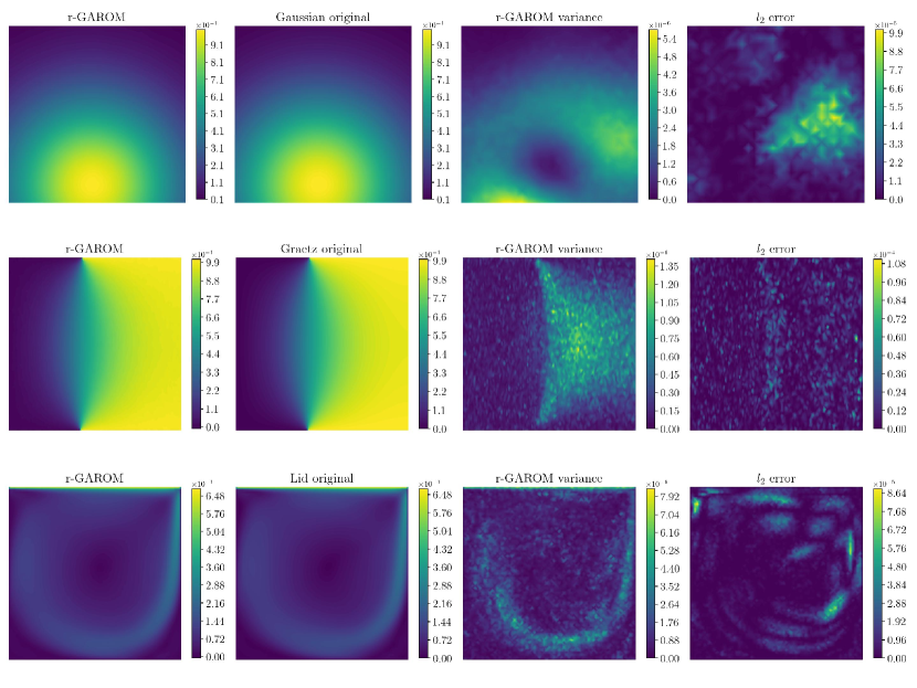
Figure 2: r-GAROM inference results. The images show the generated snapshot for a testing parameter using a latent dimension of $64$, compared to the corresponding high-fidelity solution. Top: Gaussian dataset. Center: Graetz dataset. Bottom: Lid cavity dataset.

Looking at a more precise measure for the GAROM accuracy, we calculate the mean $l_{2}$ relative error over a set of training and testing parameters, comparing it with the error obtained using the ROM baseline models — POD–RBF, POD–NN, AE–RBF, AE–NN. As we can note from Table 2, for the majority of the experiments POD–RBF is the best across all models on the training dataset (gray rows), but it fails to properly generalize to test data. Indeed, the test error for the POD (white rows) can increase drastically to more than five orders of magnitude, as in the Graetz case, showing a poor ability to correctly generalize. Differently, ML-based methodologies exhibit comparable train and test errors, due to their ability to learn complex nonlinear relationships by the data. For the test error, which is used to assess the model prediction ability, the r-GAROM model obtains very promising results for almost half of the test cases. Across the different deep learning models, r-GAROM obtains lower error for seven out of nine tests, highlighting its encouraging precision even in this preliminary contribution. It is also important to highlight that the (r-)GAROM architecture is fairly simple in all the numerical tests here pursued: both generator and discriminator are composed only of a few dense layers (details in Section 2.8). Searching for the optimal architecture is outside the scope of the work, whose aims are limited to presenting a new methodology for reduced order modeling. Because of this consideration and assuming the precision of the network is correlated to the number of hyperparameters, we suppose the accuracy can be further improved by using more powerful deep learning architectures, as in [29, 10, 25], at the cost of longer and more expensive training.

Table 2: Accuracy comparison for different test cases, methods, and latent dimensions. The table reports the mean $l_{2}$ relative error $\epsilon$ (in percent). Gray rows represent the error on training data, while white rows the error on testing data. For GAROM and r-GAROM models, also the predictive standard deviation is reported (in percent). We employ $N=240$ for Gaussian and Lid Cavity datasets, and $N=160$ for the Graetz dataset.

Method	Gaussian			Graetz			Lid Cavity
	4	16	64	16	64	120	16	64	120
GAROM	$(3.67\pm 0.47)$	$(3.52\pm 0.46)$	$(4.07\pm 0.47)$	$(0.58\pm 0.16)$	$(0.55\pm 0.14)$	$(0.51\pm 0.1)$	$(10.7\pm 0.22)$	$(9.50\pm 0.15)$	$(9.91\pm 0.17)$
r-GAROM	$\mathbf{(0.82\pm 0.15)}$	$(0.74\pm 0.13)$	$(0.74\pm 0.13)$	$\mathbf{(0.34\pm 0.05)}$	$\mathbf{(0.34\pm 0.04)}$	$\mathbf{(0.28\pm 0.04)}$	$(5.43\pm 0.08)$	$(5.04\pm 0.11)$	$(5.34\pm 0.15)$
POD–RBF	$15.4$	$\mathbf{0.41}$	$\mathbf{0.25}$	$0.48$	$0.48$	$0.49$	$\mathbf{2.98}$	$\mathbf{1.45}$	$\mathbf{1.32}$
POD–NN	$15.4$	$1.41$	$1.32$	$0.41$	$0.47$	$0.44$	$3.68$	$3.81$	$5.34$
AE–RBF	$3.10$	$2.30$	$1.82$	$1.08$	$1.42$	$1.60$	$13.9$	$8.92$	$9.32$
AE–NN	$1.76$	$1.87$	$1.84$	$1.14$	$1.56$	$2.71$	$15.5$	$9.92$	$6.21$
GAROM	$(3.64\pm 0.03)$	$(3.50\pm 0.03)$	$(3.89\pm 0.03)$	$(0.69\pm 0.01)$	$(0.62\pm 0.01)$	$(0.57\pm 0.01)$	$(13.5\pm 0.01)$	$(11.5\pm 0.01)$	$(12.6\pm 0.01)$
r-GAROM	$\mathbf{(0.78\pm 0.01)}$	$(0.74\pm 0.01)$	$(0.71\pm 0.01)$	$(0.40\pm 0.004)$	$(0.35\pm 0.004)$	$(0.25\pm 0.003)$	$(6.26\pm 0.01)$	$(5.94\pm 0.01)$	$(6.41\pm 0.01)$
POD–RBF	$15.2$	$\mathbf{0.23}$	$\mathbf{2.85\cdot 10^{-5}}$	$\mathbf{7.73\cdot 10^{-4}}$	$\mathbf{1.51\cdot 10^{-11}}$	$\mathbf{2.80\cdot 10^{-12}}$	$\mathbf{2.37}$	$\mathbf{0.29}$	$\mathbf{0.04}$
POD–NN	$15.2$	$0.82$	$1.32$	$0.36$	$0.38$	$0.40$	$3.84$	$4.16$	$6.08$
AE–RBF	$2.90$	$2.12$	$1.82$	$1.01$	$1.41$	$1.54$	$17.6$	$11.0$	$11.6$
AE–NN	$1.40$	$1.41$	$1.84$	$1.16$	$1.67$	$2.78$	$19.9$	$12.6$	$7.06$
								Training	Testing

Finally, the r-GAROM error seems to be almost independent of the latent dimension, since only a small variation of the errors is observed in training and testing for the various dimensions. In such a way, we can empirically prove the better capability to reduce the original dimension of the snapshots, since adding new reduced dimensions does not really affect the final accuracy.

3.2 Model variance

Figure 2 reports the (r-)GAROM variance obtained by a Monte Carlo approximation with different random inputs for the generator. Contrary to the ROM baseline models, GAROM can provide also an estimate of the model variance, obtained by a probabilistic ensemble (see Section 2.3). Since the solution is unique by assumption, we expect a zero variance for the generated samples given the conditioning variables. Hence, a high variance in the GAROM estimate gives an uncertain prediction of the model. This is confirmed by observing the variances for different models in Table 2, and the point-wise variance in Figure 2. Both GAROM and r-GAROM models report a small variance, with training variance always one or two orders of magnitude smaller than the testing one. This indicates that GAROM models are more uncertain in predicting testing data than training ones. This is expected since the GAROM model builds a distribution on the training data. However, it is worth noticing that the $l_{2}$ errors between training and testing in Table 2 are almost always identical across different dimensions, showing good generalizability of the model, as also reported in Section 3.3. It is evident from Table 2 that r-GAROM has a lower variance than GAROM for testing and training. This is mainly due to the regularizer term, which forces the network to converge faster, as explained in the Section 2.

The variance estimate, although very important for the aforementioned reasons, does not give a quantification of the predictive uncertainty, but only statistical information of the learnt distribution. Nevertheless, due to the probabilistic framework adopted, we can obtain bounds in probability for the reconstruction error by using the variance estimate. Indeed, as deeply explained in Section 2.4, with the variance information provided by the GAROM framework, it is possible to obtain prediction uncertainty using the Markov inequality, or the confidence interval theory. While extremely important, in this work we just show how to obtain these näive bounds. Exploring further to obtain tighter bounds, or employ the uncertainty quantification strategies for noisy data are possible new interesting research topics, which we will explore in the future.

3.3 Generalization

One fundamental aspect, especially in the context of data-driven modelling, is the ability to correctly generalize across new instances of the conditioning domain, which of course were not inside the training dataset. To empirically prove the GAROM ability to generalize over the testing parameters, we define the difference $\delta(\mathbf{c})$ as the mean difference between the truth parametric solution and the corresponding GAROM prediction, such that:

$$\delta(\mathbf{c})=\frac{1}{N_{u}}\sum_{i=1}^{N_{u}}(u_{i}(\mathbf{c})-\hat{u}_{i}(\mathbf{c})),$$ (3.3.1)

where $\mathbf{u}(\mathbf{c})=\begin{bmatrix}u_{1}(\mathbf{c})&\dots&u_{N_{u}}(\mathbf{c})\end{bmatrix}$ and $\hat{\mathbf{u}}(\mathbf{c})=\begin{bmatrix}\hat{u}_{1}(\mathbf{c})&\dots&\hat{u}_{N_{u}}(\mathbf{c})\end{bmatrix}$. We highlight that we do not consider the absolute value here in order to detect possible systematic over- and under-estimations of the proposed model.

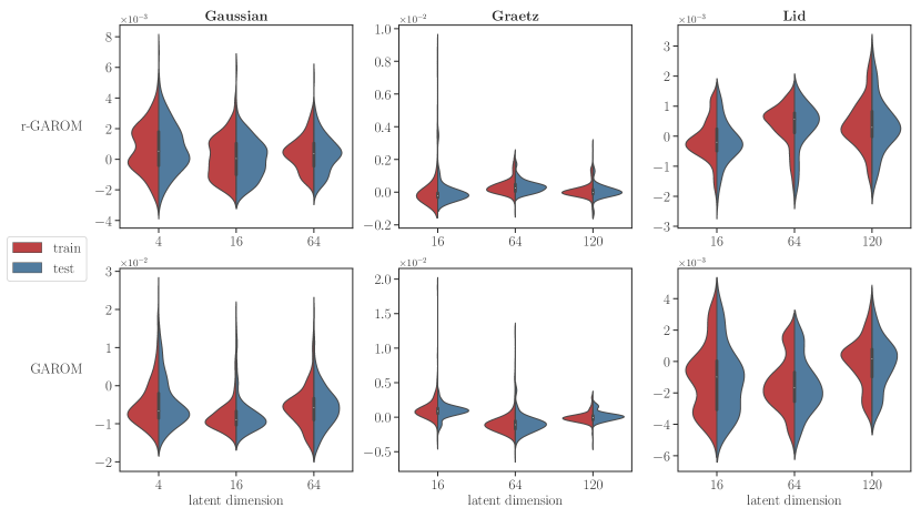
Figure 3: Distribution of the $\delta$ difference. The graph depicts, for each latent dimension, train (red) and test (blue) distribution of the $\delta$. Top: r-GAROM model. Bottom: GAROM model.

Figure 3 shows the distribution of the $\delta$ different for all latent dimensions and for all test cases. We can note that the distribution of the error computed over the training parameters is quite similar to the error distribution for the testing parameters in all the numerical investigations. Such behaviour indicates that both models can correctly generalize outside the training dataset, for the proposed problems. Furthermore, the distributions are centered around zero for both models, indicating a good high-fidelity solution reconstruction, as also shown in the previous Section. Finally, it is worth noticing that r-GAROM distributions are more closed towards zero than the not regularized counterpart, as a consequence of the regularizer term addition.

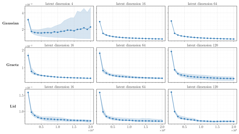
Figure 4: r-GAROM convergence graph in $l_{2}$ relative error for multiple training. The solid line indicates the average across all simulations. The shaded area represents the interval obtained by taking the maximum and minimum error across all simulations. The total number of training is $5$.

3.4 Robustness

The last investigation regards the robustness of the training. It is well established in the deep learning community that generative adversarial networks tend to be unstable during training [15]. Nevertheless, such behaviour is drastically reduced with BEGAN [6, 28]. In order to assess the convergence of the optimization procedure, we perform a statistical analysis studying the error trend during the training, using different random initialization for the weights of the network. Practically, $5$ training loops are carried out changing the seed for the random number generator. Figure 4 depicts the mean error and the interval between the minimum and the maximum error across the 5 simulations. The plot indicates a stable convergence of r-GAROM, with sporadic perturbations in the statistical campaign. The unique test case that is showing not a stable trend is the Gaussian one, but only when the latent dimension is $4$: we suppose the latent dimension is not sufficiently big to represent the original problem, leading to an aleatory optimization. However, the $l_{2}$ relative error for the maximum discrepancy is in the same order of magnitude as the average result, showing that the model has still reached a good performance.

4 Discussion

In this study, we proposed GAROM, a generative adversarial reduce order modeling approach to tackle parametric PDE problems. The presented methodology is also extended to a regularized version (r-GAROM) in case the solution for the PDE is unique. The methodology is general, and applicable to a variety of ROM problems. The latter is tested on three parametric benchmarks for different latent dimensions, showing very promising results in data-driven modeling. Among the deep learning approaches for ROM, r-GAROM outperforms in terms of accuracy in model prediction all of them in seven out of nine tests. Moreover, this approach seems to be more resilient to overfitting. The POD demonstrates again here its great robustness and applicability in ROM methods, but it emerges in these examples the high difference between train and test errors in the case the POD is not able to properly detect the latent dimension of the problem — e.g. due to nonlinearity. Differently, GAROM and its variation do not suffer from poor generalization, resulting in a more reliable model, despite the lack of precision in some tests. Surprisingly, it also shows any dependence between the $l_{2}$ relative mean error and the latent dimension we use in the discriminator, making it less sensitive to this parameter. It must be repeated that, with the GAROM approach, we are not projecting data on a reduced space, but the inner dimension is only used in the discriminator autoencoder. The adversarial approach combined with the proposed regularisation seems also helpful to stabilize the training in terms of loss trend, making such an approach practically less difficult to hyper-parameters tuning. Finally, the statistical approach allows to compute the variance learned by the generator, making it possible to quantify the uncertainty of predictions applying different statistical strategies.

We identify multiple exciting research directions for the methodology. Firstly, improving the quality of the neural networks for the generator, discriminator, and conditioning mechanisms, and applying the methodology to more complex problems. As already stated, in the work we have used very simple architectures, which limits the generation capability. As an example, the framework could be easily extended to time-dependent problems, employing LSTM [19] or transformers [44] networks for the conditioning mechanism. Alternatively, as also suggested in [6], employing different architecture for the discriminator, e.g. U-net [38], could lead to accuracy improvement. Another possibility is to enhance the conditioning set with more information, e.g. by passing POD modes, or mesh information. Another very interesting prosecution of this work would be the continuous extension of the entire architecture. With the proposed one, both the networks’ dimension scales with the number of components in the snapshots vector. To apply such approach to very finer meshes, the computational requirement to train and infer the model would be huge and sometimes unfeasible. In these cases, a spatial continuous extension can lead to a wider diffusion, especially in more complex problems. Another possibility to mitigate the difficult application to finer meshes (and so snapshots with more degree of freedom) is the employment of the architecture presented in [8] where the authors employ continuous convolutional neural networks over unstructured meshes.

In summary, the presented new methodology, combined with the different new research directions, paves the way to the application of GAROM in very complex settings, exhibiting great potential for future ROM developments in computational science.

5 Acknowledgements

This work is partially supported by European Union Funding for Research and Innovation — Horizon 2020 Program — in the framework of European Research Council Executive Agency: H2020 ERC CoG 2015 AROMA-CFD project 681447 ”Advanced Reduced Order Methods with Applications in Computational Fluid Dynamics” P.I. Professor Gianluigi Rozza, by European Union Funding for Research and Innovation — Horizon Europe Program — in the framework of European Research Council Executive Agency: ERC POC 2022 ARGOS project 101069319 “Advanced Reduced order modellinG: Online computational web server for complex parametric Systems” P.I. Professor Gianluigi Rozza, by European High-Performance Computing Joint Undertaking project Eflows4HPC GA N. 955558, by PRIN ”Numerical Analysis for Full and Reduced Order Methods for Partial Differential Equations” (NA-FROM-PDEs) project.

References

- [1] OpenFOAM. (Accessed on 07/09/2022).
- [2] G. N. W. e. a. A. Logg, K.-A. Mardal. Automated Solution of Differential Equations by the Finite Element Method. Springer, 2012.
- [3] M. Arjovsky, S. Chintala, and L. Bottou. Wasserstein generative adversarial networks. In International conference on machine learning, pages 214–223. PMLR, 2017.
- [4] P. Bauer, A. Thorpe, and G. Brunet. The quiet revolution of numerical weather prediction. Nature, 525(7567):47–55, 2015.
- [5] G. Berkooz, P. Holmes, and J. L. Lumley. The proper orthogonal decomposition in the analysis of turbulent flows. Annual review of fluid mechanics, 25(1):539–575, 1993.
- [6] D. Berthelot, T. Schumm, and L. Metz. Began: Boundary equilibrium generative adversarial networks. arXiv preprint arXiv:1703.10717, 2017.
- [7] C. M. Bishop. Latent variable models. Learning in graphical models, 371, 1998.
- [8] D. Coscia, L. Meneghetti, N. Demo, G. Stabile, and G. Rozza. A continuous convolutional trainable filter for modelling unstructured data. Computational Mechanics, pages 1–13, 2023.
- [9] N. Demo, M. Tezzele, and G. Rozza. Ezyrb: Easy reduced basis method. Journal of Open Source Software, 3(24):661, 2018.
- [10] S. Dutta, P. Rivera-Casillas, B. Styles, and M. W. Farthing. Reduced order modeling using advection-aware autoencoders. Mathematical and Computational Applications, 27(3):34, 2022.
- [11] H. Eivazi, S. Le Clainche, S. Hoyas, and R. Vinuesa. Towards extraction of orthogonal and parsimonious non-linear modes from turbulent flows. Expert Systems with Applications, 202:117038, 2022.
- [12] H. Eivazi, H. Veisi, M. H. Naderi, and V. Esfahanian. Deep neural networks for nonlinear model order reduction of unsteady flows. Physics of Fluids, 32(10):105104, 2020.
- [13] I. C. Gonnella, M. W. Hess, G. Stabile, and G. Rozza. A two stages deep learning architecture for model reduction of parametric time-dependent problems. arXiv preprint arXiv:2301.09926, 2023.
- [14] I. Goodfellow, Y. Bengio, and A. Courville. Deep learning. MIT press, 2016.
- [15] I. Goodfellow, J. Pouget-Abadie, M. Mirza, B. Xu, D. Warde-Farley, S. Ozair, A. Courville, and Y. Bengio. Generative adversarial networks. Communications of the ACM, 63(11):139–144, 2020.
- [16] K. Gundersen, A. Oleynik, N. Blaser, and G. Alendal. Semi-conditional variational auto-encoder for flow reconstruction and uncertainty quantification from limited observations. Physics of Fluids, 33(1):017119, 2021.
- [17] J. S. Hesthaven, G. Rozza, B. Stamm, et al. Certified reduced basis methods for parametrized partial differential equations, volume 590. Springer, 2016.
- [18] J. S. Hesthaven and S. Ubbiali. Non-intrusive reduced order modeling of nonlinear problems using neural networks. Journal of Computational Physics, 363:55–78, 2018.
- [19] S. Hochreiter and J. Schmidhuber. Long short-term memory. Neural computation, 9(8):1735–1780, 1997.
- [20] M. Ilse, J. M. Tomczak, C. Louizos, and M. Welling. Diva: Domain invariant variational autoencoders. In Medical Imaging with Deep Learning, pages 322–348. PMLR, 2020.
- [21] D. P. Kingma and J. Ba. Adam: A method for stochastic optimization. arXiv preprint arXiv:1412.6980, 2014.
- [22] D. P. Kingma and M. Welling. Auto-encoding variational bayes. arXiv preprint arXiv:1312.6114, 2013.
- [23] T. Lassila, A. Manzoni, A. Quarteroni, and G. Rozza. Model order reduction in fluid dynamics: challenges and perspectives. Reduced Order Methods for modeling and computational reduction, pages 235–273, 2014.
- [24] D. Lazzaro and L. B. Montefusco. Radial basis functions for the multivariate interpolation of large scattered data sets. Journal of Computational and Applied Mathematics, 140(1-2):521–536, 2002.
- [25] K. Lee and K. T. Carlberg. Model reduction of dynamical systems on nonlinear manifolds using deep convolutional autoencoders. Journal of Computational Physics, 404:108973, 2020.
- [26] H. Lomax, T. H. Pulliam, D. W. Zingg, T. H. Pulliam, and D. W. Zingg. Fundamentals of computational fluid dynamics, volume 246. Springer, 2001.
- [27] D. J. Lucia, P. S. Beran, and W. A. Silva. Reduced-order modeling: new approaches for computational physics. Progress in aerospace sciences, 40(1-2):51–117, 2004.
- [28] A. Marzouk, P. Barros, M. Eppe, and S. Wermter. The conditional boundary equilibrium generative adversarial network and its application to facial attributes. In 2019 International Joint Conference on Neural Networks (IJCNN), pages 1–7. IEEE, 2019.
- [29] R. Maulik, B. Lusch, and P. Balaprakash. Reduced-order modeling of advection-dominated systems with recurrent neural networks and convolutional autoencoders. Physics of Fluids, 33(3):037106, 2021.
- [30] A. T. Mohan and D. V. Gaitonde. A deep learning based approach to reduced order modeling for turbulent flow control using lstm neural networks. arXiv preprint arXiv:1804.09269, 2018.
- [31] A. v. d. Oord, S. Dieleman, H. Zen, K. Simonyan, O. Vinyals, A. Graves, N. Kalchbrenner, A. Senior, and K. Kavukcuoglu. Wavenet: A generative model for raw audio. arXiv preprint arXiv:1609.03499, 2016.
- [32] A. Paszke, S. Gross, F. Massa, A. Lerer, J. Bradbury, G. Chanan, T. Killeen, Z. Lin, N. Gimelshein, L. Antiga, A. Desmaison, A. Kopf, E. Yang, Z. DeVito, M. Raison, A. Tejani, S. Chilamkurthy, B. Steiner, L. Fang, J. Bai, and S. Chintala. Pytorch: An imperative style, high-performance deep learning library. Advances in neural information processing systems, 32, 2019.
- [33] A. Razavi, A. Van den Oord, and O. Vinyals. Generating diverse high-fidelity images with vq-vae-2. Advances in neural information processing systems, 32, 2019.
- [34] S. Reed, Z. Akata, X. Yan, L. Logeswaran, B. Schiele, and H. Lee. Generative adversarial text to image synthesis. In International conference on machine learning, pages 1060–1069. PMLR, 2016.
- [35] D. J. Rezende and F. Viola. Taming vaes. arXiv preprint arXiv:1810.00597, 2018.
- [36] S. Rifai, P. Vincent, X. Muller, X. Glorot, and Y. Bengio. Contractive auto-encoders: Explicit invariance during feature extraction. In Proceedings of the 28th international conference on international conference on machine learning, pages 833–840, 2011.
- [37] R. Rombach, A. Blattmann, D. Lorenz, P. Esser, and B. Ommer. High-resolution image synthesis with latent diffusion models. In Proceedings of the IEEE/CVF Conference on Computer Vision and Pattern Recognition, pages 10684–10695, 2022.
- [38] O. Ronneberger, P. Fischer, and T. Brox. U-net: Convolutional networks for biomedical image segmentation. In Medical Image Computing and Computer-Assisted Intervention–MICCAI 2015: 18th International Conference, Munich, Germany, October 5-9, 2015, Proceedings, Part III 18, pages 234–241. Springer, 2015.
- [39] G. Rozza, G. Stabile, and F. Ballarin. Advanced Reduced Order Methods and Applications in Computational Fluid Dynamics. SIAM, 2022.
- [40] R. Schreiber and H. B. Keller. Driven cavity flows by efficient numerical techniques. Journal of Computational Physics, 49(2):310–333, 1983.
- [41] A. Solera-Rico, C. S. Vila, M. Gómez, Y. Wang, A. Almashjary, S. Dawson, and R. Vinuesa. -variational autoencoders and transformers for reduced-order modelling of fluid flows. arXiv preprint arXiv:2304.03571, 2023.
- [42] W. A. Strauss. Partial differential equations: An introduction. John Wiley & Sons, 2007.
- [43] J. M. Tomczak. Deep generative modeling. Springer, 2022.
- [44] A. Vaswani, N. Shazeer, N. Parmar, J. Uszkoreit, L. Jones, A. N. Gomez, Ł. Kaiser, and I. Polosukhin. Attention is all you need. Advances in neural information processing systems, 30, 2017.
- [45] P. Vincent, H. Larochelle, Y. Bengio, and P.-A. Manzagol. Extracting and composing robust features with denoising autoencoders. In Proceedings of the 25th international conference on Machine learning, pages 1096–1103, 2008.
- [46] Y. Yang and P. Perdikaris. Adversarial uncertainty quantification in physics-informed neural networks. Journal of Computational Physics, 394:136–152, 2019.