Robust asymptotic observer of motion states with nonlinear friction

Abstract

This paper revisits the previously proposed linear asymptotic observer of the motion state variables with nonlinear friction and provides a robust design suitable for both, transient presliding and steady-state sliding phases of the relative motion. The class of motion systems with the only measurable output displacement is considered. The reduced-order Luenberger-type observer is designed based on the obtained simplified state-space representation with a time-varying system matrix. The resulted observation error dynamics proves to be robust and appropriate for all variations of the system matrix, which are due to the nonlinear spatially-varying friction. A specially designed tribological setup to accurately monitor the relative motion between two contacting friction surfaces is used to collect the experimental data of the deceleration trajectories when excited by a series of impulses. The performance of the state estimation using the proposed observer is shown based on the collected experimental data.

1 Introduction

The observation of dynamic states in the motion systems is a long-term problem within (motion) control communities. Often, only the relative displacement of an actuated system is measured by the sensing elements, such as e.g. encoders, while the relative velocity as well as some internal dynamic states of the entire system need also to be known in real time. The classical observation strategies, like Luenberger observer (see Luenberger (1964)), disturbance observer (see e.g. Ohishi et al. (1987); Shim et al. (2016)), or sliding-mode observers (see e.g. Shtessel et al. (2014) and references therein), are well known. Also a variety of related and analogous approaches have been developed over the past three decades; several more specific references are omitted here for reasons of space and too large a number published works. One of the fundamental problems related to dynamic states of relative motion and their observation is nonlinear friction, which is present in almost all driven mechanical systems. As well known, the kinetic friction can (i) lead to the undesired and long-period stick-slip cycles in case of a feedback-controlled motion (see e.g. Ruderman (2022)), (ii) affect the motion breakaway and reversals phases (see e.g. Ruderman (2017) and Ruderman and Rachinskii (2017)), and (iii) result in unacceptable steady-state control errors (see e.g. Ruderman and Iwasaki (2016)) if it is not properly compensated. Moreover, the friction forces are well known to be not directly measurable (see e.g. Harnoy et al. (2008)) and, in addition, they are mostly uncertain due various system-internal and environment-external factors (see e.g. Ruderman and Iwasaki (2015)). A robust, like discontinuity-based, compensation of nonlinear friction (see e.g. Ruderman and Fridman (2022)) can partially solve the problem, but can have a limited acceptance in several applications due to a high-frequent relay-type control action. Therefore, it is often understood that an accurate on-line estimation of friction force values can be of great benefit to the performance of motion control systems with friction, cf. e.g. Olsson et al. (1998) and Chen et al. (2000). Since the dynamics of frictional forces are far from trivial, see e.g. Al-Bender and Swevers (2008) for a detailed tutorial, designing a reliable friction observer remains a significant challenge for the motion control and its applications. Some recent experimentally confirmed scenarios revealing the nature of frictional perturbations for motion control can be found in the literature, for instance in Beerens et al. (2019); Kim et al. (2019) just to name a few applications here. An observer-based strategy for compensating the nonlinear friction was proposed in Ruderman and Iwasaki (2015), which allowed for an accurate positioning control up to the level of encoder resolution. However, a systematic analysis of the error dynamics and, hence, observer synthesis remained partially undisclosed and less explained as methodology. The aim of this paper is to close this gap and thus to approach the observer design for motion systems with nonlinear friction in a simple and systematic way.

The rest of the paper is organized as follows. In the next section, we first formalize the problem statement by introducing the class of motion systems with nonlinear friction, for which the asymptotic Luenberger-type state observer is proposed. In the main section 3, we make assumptions about the dynamic friction state and introduce the corresponding asymptotic state observer, also providing the robust design of observer gains. The developed tribological experimental setup used in this work is described in section 4. Experimental evaluation of the proposed observer is provided in section 5. Conclusions are given in section 6.

2 Problem formulation

The following observation problem is addressed in this work. Consider the dynamic motion system

$$m\ddot{x}(t)+f\bigl{(}\dot{x}(t)\bigl{)}=u(t),$$ (1)

where an inertial mass $m$ is actuated by the input $u$ and counteracted by the nonlinear kinetic friction $f(\cdot)$. Recall that the latter appears due to the normal contacts. The available input and output signals are the drive force $u(t)$ and relative displacement $x(t)$, both in the generalized coordinates of a 1DOF system, here without distinguishing between the translational and rotational motion. The inertial mass is assumed to be accurately known, while for the nonlinear friction the following can be assumed:

1. The total kinetic friction in steady-state is a superposition of the Coulomb and viscous friction forces

   $$f(t)=F_{c}+F_{v}.$$ (2)

   The superposition (2) is consistent with the established approaches to modeling friction, especially when using the Newton-Euler dynamics equations, and also considering the Stribeck weakening effects. The superposition principle can be temporary lost during the dynamic transients, particularly at the reversals of motion, where the viscous friction effects can subside and also lose their linearity.

2. The Coulomb friction force in steady-state depends on the motion direction only, i.e.

   $$F_{c}=C_{f}\,\mathrm{sign}(\dot{x}),$$ (3)

   and is parameterized by an uncertain Coulomb coefficient, for which a nominal value $C_{f}>0$ is known.

3. The viscous friction force depends linearly on the relative displacement rate only, i.e.

   $$F_{v}=\sigma\,\dot{x}.$$ (4)

   The proportional friction law constitutes the standard linear system damping and is parameterized by the (generally) uncertain viscous friction coefficient, for which the nominal value $\sigma>0$ is known.

4. The transient behavior of kinetic friction $f(t)$ is to a large extent unknown, while assuming two of its commonly stated properties. (a) The viscous friction term is subject to the so-called frictional lag during sufficiently large velocity rates, i.e. at high accelerations and decelerations. (b) The Coulomb friction during the so-called presliding, i.e. at the motion beginning, stop, and reversals, is not discontinuous (cf. with eq. (3)) and undergoes some smooth hysteresis-shaped transitions. These transitions are subject to uncertainties due to the spatially and temporally varying nature of the friction surfaces.

For the above system (1), with the nonlinear kinetic friction satisfying (i)–(iv), one wishes to design a robust asymptotic state observer so that the estimates of dynamic states $\dot{\tilde{x}}(t)\rightarrow\dot{x}(t)$, $\tilde{f}(t)\rightarrow f(t)$ as $t\rightarrow\infty$. The initial values of the real system states $(\dot{x},f)(0)$ are unknown. And the only available system measurements are $-\infty<\bigl{(}x(t),u(t)\bigr{)}<\infty$, both affected by the sensing noise.

3 State observer

3.1 Dynamic friction states

At fist, we have to consider both frictional terms in superposition, cf. eq. (2), as the dynamic friction states. This will enable their observation and corresponding integration into the observer scheme to be designed.

For the viscous friction term, one can write

$$\dot{F}_{v}=\beta^{-1}(\sigma\dot{x}-F_{v}),$$ (5)

instead of (4), thus capturing the so-called frictional lag, see e.g. Al-Bender and Swevers (2008) for details. Recall that the latter appear (but not necessarily as linear) in the relative $(\dot{x},F_{v})$ coordinates. One can recognize that if the time constant $\beta$ of the frictional lag is zero, then the dynamic equation (5) will collapse, and one will obtain the standard viscous damping relationship which is static, cf. with eq. (4). Here it is important to emphasize that the introduced time constant $\beta>0$ is relatively low and mostly uncertain all the time. This makes its proper identification to a sufficiently challenging task. If no nominal $\beta$ value is available, assigning an arbitrary $0<\beta\ll m\sigma^{-1}$ may suffice. This will ensure the time constant of the friction lag is significantly lower than the time constant of the mechanical drive, cf. with eq. (1).

The dynamics of the nonlinear Coulomb friction captures the presliding transition curves, this way leading to

$$\dot{F}_{c}=\left\{\begin{array}[]{ll}\dot{x}\cdot\partial F_{c}/\partial x\,,&\hbox{if }|F_{c}|<C_{f},\\[2.84526pt] 0,&\hbox{otherwise.}\\ \end{array}\right.$$ (6)

Recall that describing the Coulomb friction force which should include presliding and, therefore, avoid discontinuity at motion reversals, relies on a smooth multi-valued mapping $x\mapsto f$ within the presliding range. The latter means that the motion undergoes an onset or reversal, so that $|\dot{x}|$ is relatively low and the non-viscous friction mechanisms predominate. As long as a progressing $F_{c}(x)$-curve is not saturated at $\pm C_{f}$, the dynamic transitions (6) take place. Afterwards, the constant Coulomb friction force characterizes the steady-state, cf. with eq. (3).

Since both dynamic friction states (5), (6) act on the motion dynamics (1) simultaneously, i.e. in superposition (2), their proper decomposition can pose serious (probably unsolvable) challenge when observing them individually. Therefore, the overall dynamic friction state $f(\cdot)$ will be used next in the observer design, while assuming that the nominal value $\sigma$ and presliding map (6) are available and the parameter $\beta$ is sufficiently preestimated.

3.2 Asymptotic Luenbeger-type observer

For the class of motion systems given by (1), with the dynamic friction (2), we introduce the state vector $w\equiv(w_{1},w_{2},w_{3})^{T}:=(x,\dot{x},f)^{T}$ and derive the simplified dynamic state-space model as

$$\dot{w}=\underset{A}{\underbrace{\left(\begin{array}[]{ccc}0&1&0\\ 0&0&-1/m\\ 0&\bigl{(}\partial F_{c}/\partial x+\sigma/\beta\bigr{)}&0\end{array}\right)}}w+\underset{B}{\underbrace{\left(\begin{array}[]{c}0\\ 1/m\\ 0\end{array}\right)}}u.$$ (7)

The associated output coupling vector is $C=(1,0,0)$, since the relative displacement is the single available output value, i.e. $x=Cw$. One should notice that the system matrix $A$ has one time-dependent term $\partial F_{c}/\partial x$ so that one deals with $A(t)$ during the presliding. Outside the presliding range, the $\partial F_{c}/\partial x$ term becomes zero. On the contrary, $\partial F_{c}/\partial x\rightarrow\kappa$ after each reversal point $x(t_{r}^{+})\equiv x_{r}$, where $t_{r}$ is the time instant of the last motion reversal, and $\kappa\gg 0$ is a large positive constant representing the initial stiffness of the given frictional surface pair. Note that one can have $\kappa\rightarrow\infty$ at $t_{r}$, that is in line with temporary stiction during the motion reversals, cf. Ruderman and Rachinskii (2017). Also recall that at $t_{r}$ the sign of $\dot{x}$ changes, i.e. the system (1) either starts or stops to move, or it changes the direction of relative displacement. For both of the above cases, i.e. for $\partial F_{c}/\partial x=0$ and $\partial F_{c}/\partial x\gg 0$, the $(A,C)$-pair proves to be observable in the Kalman sense. This allows designing the standard Luenberger-type observer, cf. Luenberger (1964), so that an asymptotic convergence of the states estimation, i.e. $\tilde{w}(t)\rightarrow w(t)$, can be guaranteed.

In order to simplify the observer design and, moreover, to improve the convergence properties of $\tilde{w}(t)$, we transform the state-space representation (7) into the regular form

$$\left(\begin{array}[]{c}\dot{\bar{w}}\\ \dot{z}\\ \end{array}\right) = \left(\begin{array}[]{cc}A_{11}&A_{12}\\ A_{21}&A_{22}\end{array}\right)\left(\begin{array}[]{c}\bar{w}\\ z\\ \end{array}\right)+\left(\begin{array}[]{c}B_{\bar{w}}\\ B_{z}\\ \end{array}\right)\,u$$ (16)

$$x = \left(\begin{array}[]{cc}C_{\bar{w}}&C_{z}\\ \end{array}\right)\left(\begin{array}[]{c}\bar{w}\\ z\\ \end{array}\right),$$ (20)

where $\bar{w}=w_{1}$ and $z=(w_{2},w_{3})^{T}$. Then, we apply a standard reduced-order asymptotic observer, cf. Luenberger (1971). Recall that the above transformation of (7) into the regular form, with breakdown of $A$, $B$, $C$ into the matrices of an appropriate dimension in (16), (20), provides a separation into the measurable and unmeasurable states $\bar{w}$ and $z$, respectively. Subsequently, an exclusion of $\bar{w}$ from the estimated state vector reduces the order of the observer dynamics from three to two and, this way, the complexity of the associated poles assignment.

The reduced-order Luenberger observer is given by

$$\dot{\tilde{z}} = (A_{22}-LA_{12})\tilde{z}+$$

$$+ (A_{21}-LA_{11}+A_{22}L-LA_{12}L)\bar{w}+(B_{z}-LB_{\bar{w}})u,$$

where $L\equiv(L_{1},L_{2})^{T}$ is the vector of observer gains, which are the design parameters. Here $\tilde{z}$ is the estimate vector of the unmeasurable system states $z$. It is worth recalling that the state observer (3.2) provides an asymptotic convergence $\tilde{z}(t)\rightarrow z(t)$ under one and the single condition – the observer system matrix $(A_{22}-LA_{12})$ has to be Hurwitz. In order to transform back the dynamic state $\tilde{z}(t)$, which was input-output-scaled according to the right-hand-side of (3.2), the back-transformation

$$(\tilde{w}_{2},\tilde{w}_{3})^{T}=\tilde{z}+L\bar{w},$$ (22)

is subsequently required, cf. Luenberger (1971).

3.3 Presliding transitions

In order to capture the $\partial F_{c}/\partial x$ term, which is entering the system matrix $A$ in (7), one needs to map the continuous presliding friction transitions in the sense of $\bigl{(}x(t)-x_{r}\bigr{)}\mapsto F_{c}$. Note that a particular modeling approach can be of secondary importance when capturing the presliding friction force. Most important is rather to ensure that such mapping is (i) piecewise continuous on the interval between the reversal state $f_{r}\equiv F_{c}(t_{r})$ at $t_{r}$ and the saturated friction state $|F_{c}|=C_{f}$; (ii) the force-displacement curves are at least $\mathcal{C}^{1}$ smooth, (iii) the force-displacement curves follow the closed hysteresis loops between two reversal points and, then, they saturate at the $\pm C_{f}$ Coulomb friction level, cf. Fig. 1.

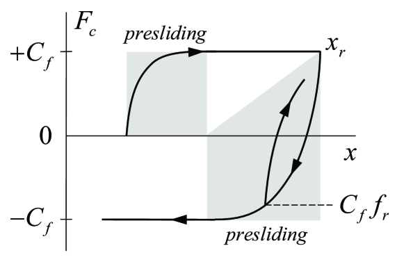
Figure 1: Presliding friction force transitions at reversals. Each change in the sign of $\dot{x}$ gives rise to a new hysteresis branch and sets the frictional system into presliding. Once the friction force saturates at $\pm C_{f}$, the hysteresis memory is erased, and the frictional system is in gross sliding.

While different fairly suitable modeling approaches (most importantly, those that have a small number of free parameters) exist, for instance the Dahl model (see Dahl (1976)) or the modified Maxwell-slip model (see Ruderman and Bertram (2011)), in this work we use an approach (see Ruderman (2017) for details) which is based on the tribological study Koizumi and Shibazaki (1984) of presliding hysteresis loops. Using the scaling factor $s>0$, which relates an after-reversal motion to the presliding distance as

$$z=s\int\limits^{t}_{t_{r}}\dot{x}\,dt,$$ (23)

and is defined on the interval $z\in[-1,\,0)\cup(0,\,1]$, one can describe the branching of friction force in presliding by

$$f_{0}(z)=z\bigl{(}1-\ln|z|\bigr{)}.$$ (24)

Recall that each motion reversal at $t_{r}$ gives rise to a new presliding transition, so that the total (normalized) presliding friction map is, cf. Ruderman (2017),

$$f_{p}(t)=\bigl{|}\mathrm{sign}(\dot{x})-f_{r}\bigr{|}\,z\bigl{(}1-\ln|z|\bigr{)}+f_{r}.$$ (25)

Note that the presliding friction dynamics memories the state of the last reversal transition, i.e. $f_{r}:=f_{p}(t_{r})$, see Fig. 1. Since the presliding mapping (25) is defined for $|z|\leq 1$ only, the entire continuous Coulomb friction law becomes, cf. with eq. (3),

$$F_{c}=\left\{\begin{array}[]{ll}C_{f}\,f_{p}(t),&\hbox{if }|z|\leq 1,\\[2.84526pt] C_{f}\,\mathrm{sign}\bigl{(}\dot{x}(t)\bigr{)},&\hbox{otherwise.}\\ \end{array}\right.$$ (26)

For the presliding distance $z$, which is linked to the output displacement by the scaling parameter $s$ and integral (23), which is reset at each $t_{r}$, one can obtain $\partial F_{c}/\partial x$ out from

$$\frac{\partial F_{c}}{\partial z}=-C_{f}\bigl{|}\mathrm{sign}(\dot{x})-f_{r}\bigr{|}\,\ln|z|.$$ (27)

3.4 Robust observer design

Recalling the time-variance of the system matrix $A$ and $A_{22}$, respectively, one can show the characteristic polynomial of the matrix $(A_{22}-LA_{12})$ to be

$$\Bigl{(}\lambda+L_{1}\Bigr{)}\lambda+\frac{1}{m}\Bigl{(}\sigma/\beta+\partial F_{c}/\partial x-L_{2}\Bigr{)}=0.$$ (28)

Obviously $\lambda$ is the complex Laplace variable so that both eigenvalues of (28) can be computed explicitly as

$$\lambda_{1,2}=\frac{1}{2}\Bigl{(}-L_{1}\pm\sqrt{L_{1}^{2}+\frac{4}{m}\bigl{(}L_{2}-\partial F_{c}/\partial x-\sigma/\beta\bigr{)}}\,\Bigr{)}.$$ (29)

Based on that, imposing the conditions

$$(\mathrm{a})\quad L_{1}>0\quad\text{ and }\quad(\mathrm{b})\quad L_{1}>2\sqrt{\frac{\kappa+\sigma/\beta-L_{2}}{m}}$$ (30)

one can ensure the observer dynamics is (i) asymptotically stable and (ii) has no complex poles, which otherwise would lead to transient oscillations. Furthermore, one can recognize that a sufficiently large $L_{1}$ will determine the most left-hand-side pole and, thus, a faster convergence of the $\tilde{w}_{2}$ estimate, which is the relative velocity. At the same time, $L_{2}$ is expected to be negative in the most cases, i.e. for $0<\sigma\ll\kappa$, so as to guarantee that (30) holds also for $\partial F_{c}/\partial x=0$. Recall that the latter characterizes the sliding phases where $F_{c}$ is already saturated. A selected ratio between the $L_{1},L_{2}$ gains, while satisfying (30), is controlling the distance between both real poles (29). This distance becomes maximal for $\partial F_{c}/\partial x=0$, and it is decreasing during the presliding as the $\partial F_{c}/\partial x$ value grows. This way, a robust observer (3.2), (22) can be realized for all phases of the nonlinear friction, also for uncertain parameters and during transient behavior of the dynamic friction, cf. sections 1 and 3.1.

4 Tribological setup

The specially designed tribological setup (see Fig. 2) consists of a linear moving platform which is placed under the mechanical frame and guides the lumped disks (from various materials). This way, an exposed disk and the linear platform have a homogenous horizontal frictional contact. The used steel disk (lacquered for a better laser reflection) with the total mass $m=52$ gram can slide over the moving platform which has an equally polished surface out of steel. The Coulomb friction coefficient is calculated as $C_{f}=\mu mg=0.2143$ N, where $g$ is the gravitational acceleration constant. The frictional coefficient $\mu$ is taken from the tribological literature for a kinetic (sliding) behavior of a clean and dry steel on steel pair. The moving platform can be actuated by a servo-drive with the stiff high-precision ball-screw, so that its linear displacement is known based on the motor encoder (not used in this work). The absolute position of the sliding disk is measured by a high-resolution laser sensor, which beam is touching the disk in its center (see Fig. 2). The diameter of the disk is only half millimeter lower than the width of the guiding slot of the frame. This way, the motion of the disk is accurately constrained from both sides, and the only one horizontal degree of freedom (i.e. denoted with the coordinate $x$) can be assumed. Lateral contacts between the disc and the walls of the frame-slot are minimized by the specially machined side-edging on the disc. Therefore, the by-effect due to the side-contact with the walls can be neglected, in comparison to the main frictional contact area of the disc which is placed on the moving platform.

Figure 2: Tribological experimental setup (laboratory view).

In this work, the decelerating trajectories of the sliding disk were used without actuating the motion platform. More specifically, a series of mechanical impulses was manually provided to the disk, while the motion platform remained non-driven. This way, the measured with the laser sensor signal $x(t)$ represents an absolute displacement of the disk, while an initial relative velocity after each new impulse is unknown. Note that the unfiltered real-time data of the disk displacement are recorded in the control board, with the sampling rate set to 2 kHz.

5 Experimental evaluation

While the overall moving mass $m$ and the Coulomb friction coefficient $C_{f}$ are assumed to be known from the available system data, cf. section 4, the residual frictional parameters $\sigma$, $\beta$, $s$ are uncertain and can only be estimated roughly, based on the (even though accurate) experimental measurements. The least-squares best fit of the modeled dynamics (1) when tuning the unknown frictional parameters in (4), (5), (23), is shown in Fig. 3.

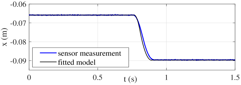
Figure 3: Measured impulse response versus the motion dynamics (1) with least-squares best fit of friction (2).

Note that the manually injected input impulse cannot be ideally executed, i.e. with a time-of-impact $\rightarrow 0$. Therefore, the measured impulse response is inherently affected by some by-effecting transient input dynamics, cf. Fig. 3, even though the impulse is also fitted in the model together with the identified parameters. Despite some visible transient discrepancy, the principal shape of the fictionally damped convergence is well captured by the modeled $f(\cdot)$, cf. later with Fig. 5 (c). This allows implementing the state-space model (7) and the asymptotic observer (3.2), (22).

The measured motion profile, shown in Fig. 4 for a sequence of manually injected mechanical impulses, is used for evaluating the designed observer.

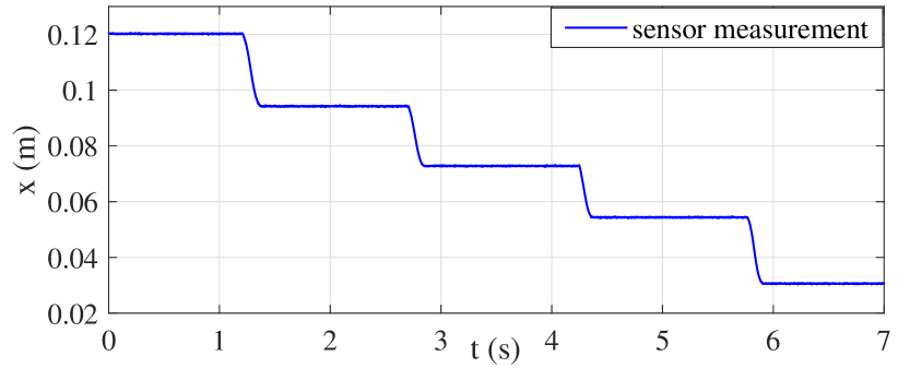
Figure 4: Relative motion of the sliding disk: measured displacement in response to the series of impulses.

Note that the applied impulses provide a series of unknown disturbing initial conditions, for which the robust observer has to converge fast enough during the relatively short periods of non-zero velocity, cf. Fig. 4. It is also important to notice that the excited motion steps are distributed over the entire length of the sliding surface of the supporting platform. This results in the varying, correspondingly uncertain, parameters of the frictional behavior, depending on spatial properties of the contact surface.

The assigned poles of the observer are $\lambda_{1,2}=(-350,-10)$. These result in the feedback gain values $L^{T}=(360,-182)$. The evaluated observer performance is demonstrated in Fig. 5. The $\tilde{w}_{3}$-estimate, which is the observed dynamic friction state, is compared with the model-predicted Coulomb friction force in the diagram (a). Note that the high-frequency pattern below the $C_{f}$-level is not discontinuous, and it constitutes a smooth pres-sliding friction behavior driven by the noisy $\bar{w}(t)$ and $\tilde{w}_{2}(t)$ values. The corresponding $\tilde{w}_{2}$-estimate of the relative velocity is shown in the diagram (b), cf. with the measured motion profile from Fig. 4. The estimated velocity peaks are clearly visible despite the noise of displacement measurement is propagated into the $\tilde{w}_{2}(t)$ signal. For a further assessment of the observer performance, the position error is compared between the nominal model, i.e.

$$e_{model}=\bar{w}-x,$$

where $x$ is predicted based on (1), and the observer-based

$$e_{obs}=\bar{w}-\int\tilde{w}_{2}\,dt,$$

where $\tilde{w}_{2}$ is the velocity estimate. Despite the integrative behavior, the $e_{obs}(t)$ is clearly superior comparing to $e_{model}(t)$, especially during the transients of non-zero velocities, as it is visible in the diagram (c). This speaks further in favor of the $(\tilde{w}_{2},\tilde{w}_{3})(t)$ estimate.

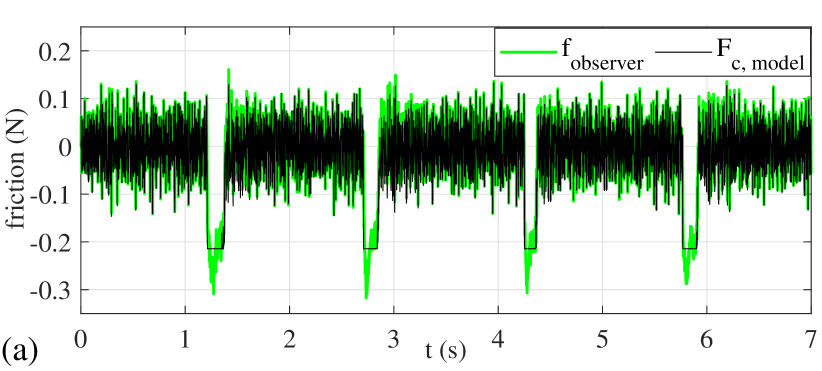
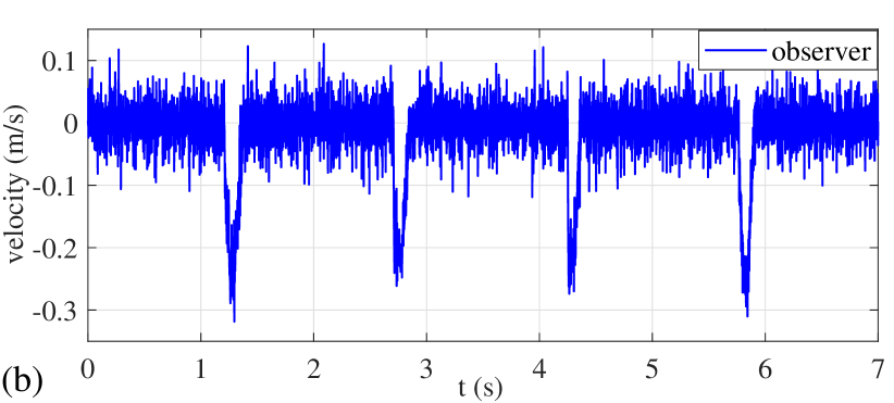
Figure 5: Observer evaluation: model-predicted $F_{c}$ versus observed $\tilde{w}_{3}$ (a), observed $\tilde{w}_{2}$ (b), model-predicted position error $e_{model}$ versus observer error $e_{obs}$ (c).

6 Conclusions

A simple and robust asymptotic observer of the nonlinear friction state is provided. Using the derived time-varying state-space notation of the motion dynamics and reduced-order Luenberger observer, it is shown that both dynamic states of the relative velocity and overall nonlinear friction force can be estimated sufficiently fast and accurately. In particular, the estimation is feasible for both, the transient presliding and sliding phases of an excited and damped relative motion. The observer provided can be parameterized by a simple and straightforward pole placement manner, which makes it well accessible for standard control engineering applications. An experimental evaluation was demonstrated on a specially designed tribological setup of moving bodies on a sliding surface. The relatively short motion instances, excited by a series of the external force-impulses, where used as a challenging scenario of relative motion in the transient phase.

References

- Al-Bender and Swevers [2008] Al-Bender, F. and Swevers, J. (2008). Characterization of friction force dynamics. IEEE Control Systems Magazine, 28(6), 64–81.
- Armstrong-Hélouvry et al. [1994] Armstrong-Hélouvry, B., Dupont, P., and De Wit, C.C. (1994). A survey of models, analysis tools and compensation methods for the control of machines with friction. Automatica, 30(7), 1083–1138.
- Beerens et al. [2019] Beerens, R., Bisoffi, A., Zaccarian, L., Heemels, W., Nijmeijer, H., and van de Wouw, N. (2019). Reset integral control for improved settling of PID-based motion systems with friction. Automatica, 107, 483–492.
- Chen et al. [2000] Chen, W.H., Ballance, D.J., Gawthrop, P.J., and O’Reilly, J. (2000). A nonlinear disturbance observer for robotic manipulators. IEEE Trans. on Industrial Electronics, 47(4), 932–938.
- Dahl [1976] Dahl, P.R. (1976). Solid friction damping of mechanical vibrations. AIAA Journal, 14(12), 1675–1682.
- Harnoy et al. [2008] Harnoy, A., Friedland, B., and Cohn, S. (2008). Modeling and measuring friction effects. IEEE Control Systems Magazine, 28(6), 82–91.
- Kim et al. [2019] Kim, M.J., Beck, F., Ott, C., and Albu-Schäffer, A. (2019). Model-free friction observers for flexible joint robots with torque measurements. IEEE Trans. on Robotics, 35(6), 1508–1515.
- Koizumi and Shibazaki [1984] Koizumi, T. and Shibazaki, H. (1984). A study of the relationships governing starting rolling friction. Wear, 93(3), 281–290.
- Luenberger [1971] Luenberger, D. (1971). An introduction to observers. IEEE Trans. on Automatic Control, 16(6), 596–602.
- Luenberger [1964] Luenberger, D.G. (1964). Observing the state of a linear system. IEEE Trans. on Military Elect., 8(2), 74–80.
- Ohishi et al. [1987] Ohishi, K., Nakao, M., Ohnishi, K., and Miyachi, K. (1987). Microprocessor-controlled dc motor for load-insensitive position servo system. IEEE Trans. on Industrial Electronics, (1), 44–49.
- Olsson et al. [1998] Olsson, H., Åström, K., de Wit, C.C., Gäfvert, M., and Lischinsky, P. (1998). Friction models and friction compensation. Eur. Journal of Control, 4(3), 176–195.
- Ruderman [2017] Ruderman, M. (2017). On break-away forces in actuated motion systems with nonlinear friction. Mechatronics, 44, 1–5.
- Ruderman [2022] Ruderman, M. (2022). Stick-slip and convergence of feedback-controlled systems with Coulomb friction. Asian Journal of Control, 24(6), 2877–2887.
- Ruderman and Bertram [2011] Ruderman, M. and Bertram, T. (2011). Modified Maxwell-slip model of presliding friction. IFAC Proceedings Volumes, 44(1), 10764–10769.
- Ruderman and Fridman [2022] Ruderman, M. and Fridman, L. (2022). Analysis of relay-based feedback compensation of Coulomb friction. In IEEE 16th International Workshop on Variable Structure Systems (VSS), 95–100.
- Ruderman and Iwasaki [2015] Ruderman, M. and Iwasaki, M. (2015). Observer of nonlinear friction dynamics for motion control. IEEE Trans. on Industrial Electronics, 62(9), 5941–5949.
- Ruderman and Iwasaki [2016] Ruderman, M. and Iwasaki, M. (2016). Analysis of linear feedback position control in presence of presliding friction. IEEJ Jour. of Ind. Applications, 5(2), 61–68.
- Ruderman and Rachinskii [2017] Ruderman, M. and Rachinskii, D. (2017). Use of Prandtl-Ishlinskii hysteresis operators for Coulomb friction modeling with presliding. In Journal of Physics: Conference Series, volume 811, 012013.
- Shim et al. [2016] Shim, H., Park, G., Joo, Y., Back, J., and Jo, N.H. (2016). Yet another tutorial of disturbance observer: robust stabilization and recovery of nominal performance. Control Theory and Technology, 14(3), 237–249.
- Shtessel et al. [2014] Shtessel, Y., Edwards, C., Fridman, L., and Levant, A. (2014). Sliding mode control and observation. Springer.