Random-anisotropy mixed-spin Ising on a triangular lattice

Abstract

We have studied the mixed spin-1/2 and 1 Ising ferrimagnetic system with a random anisotropy on a triangular lattice with three interpenetrating sublattices $A$, $B$, and $C$. The spins on the sublattices are represented by $\sigma_{A}$ (states $\pm 1/2$), $\sigma_{B}$ (states $\pm 1/2$), and $S_{C}$ (states $\pm 1$, $0$). We have performed Monte Carlo simulations to obtain the phase diagram temperature $k_{\text{B}}T/\left|J\right|$ versus the strength of the random anisotropy $D/\left|J\right|$. The phase boundary between two ferrimagnetic $FR_{1}$ and $FR_{2}$ phases at lower temperatures are always first-order for $p<0.25$ and second-order phase transition between the $FR_{1}$, $FR_{2}$ and the paramagnetic $P$ phases. On the other hand, for values of $p\gtrapprox 0.5$, the phase diagram presents only second-order phase transition lines.

Key words: random anisotropy, mixed-spin Ising system, Monte Carlo simulation

Abstract

Äîñëiäæåíî ôåððiìàãíiòíó ñèñòåìó ñóìiøi Içèíãîâèõ ñïiíiâ-1/2 òà 1 iç âèïàäêîâîþ àíiçîòðîïiєþ íà òðèêóòíié ґðàòöi ç òðüîìà âçàєìîïðîíèêàþчèìè ïiäґðàòêàìè $A$, $B$ òà $C$. Ñïiíè íà ïiäґðàòêàõ çàäàþòüñÿ ÿê $\sigma_{A}$ (ñòàíè $\pm 1/2$), $\sigma_{B}$ (ñòàíè $\pm 1/2$), òà $S_{C}$ (ñòàíè $\pm 1$, 0). Ïðîâåäåíî ìîäåëþâàííÿ Ìîíòå-Êàðëî äëÿ îòðèìàííÿ ôàçîâî¿ äiàãðàìè ‘‘òåìïåðàòóðà $k_{\text{B}}T/\left|J\right|$ – âèïàäêîâà àíiçîòðîïiÿ $D/\left|J\right|$’’. Ìåæà ðîçäiëó ìiæ äâîìà ôåððiìàãíiòíèìè ôàçàìè $FR_{1}$ òà $FR_{2}$ çà íèæчèõ òåìïåðàòóð çàâæäè âiäïîâiäàє ôàçîâîìó ïåðåõîäó ïåðøîãî (äëÿ $p<0,25$) òà äðóãîãî ðîäó (ìiæ $FR_{1}$, $FR_{2}$ òà ïàðàìàãíiòíîþ $P$ ôàçàìè). Ç iíøîãî áîêó, äëÿ çíàчåíü $p\gtrapprox 0.5$ ôàçîâà äiàãðàìà ìiñòèòü ëèøå ëiíi¿ ôàçîâèõ ïåðåõîäiâ äðóãîãî ðîäó.

Ключовi слова: âèïàäêîâà àíiçîòðîïiÿ, ñèñòåìè Içèíãà çi çìiøàíèìè ñïiíàìè, ìîäåëþâàííÿ Ìîíòå-Êàðëî

1 Introduction

Many condensed matter researchers have studied models that describe static magnetism in different materials. One of these models is the well-known mixed-spin Ising model which can describe ferrimagnetic materials [1, 2, 3]. The interest in the study of ferrimagnetic materials is due to their potential technological applications [4] which is a consequence of this material exhibiting a compensation temperature ($T_{\text{comp}}$). This phenomenon occurs when the total magnetization is zero at a temperature lower than the critical temperature ($T_{c}$).

The mixed-spin model can model the ferrimagnetic materials because they are made up of repetitions of two different atoms with spins of different magnitudes coupled antiferromagnetically each on a sublattice. Your possible ground state can be that with all spins aligned antiferromagnetically with a total magnetization greater than zero. The phase transition from the ordered (ferrimagnetic) to the disordered (paramagnetic) state occurs when the two sublattice magnetizations are zero (total magnetization is zero) at a critical temperature $T_{c}$. On the other hand, we have another interesting situation where the total magnetization can also be zero when the two sublattice magnetizations are non-zero, i.e., the sum of both is zero. This point is known as the compensation point ($T_{\text{comp}}$) and occurs at a temperature smaller than the critical temperature ($T_{\text{comp}}<T_{c}$). Kaneyoshi et al. [5, 6] and Plascak et al. [7] performed theoretical studies to understand the influence of the anisotropy on the magnetic properties and the compensation temperature in ferrimagnetic materials.

There are a lot of studies carried out with different combinations of spins, such as exact solutions [8, 9, 10, 11] for the simplest combination spin-1/2 and 1. Moreover, the mixed-spin Ising model has been studied by different approaches such as mean-field approximation [12, 13, 14, 15, 16, 17], effective-field theory [18, 19, 20, 21], re-normalization group [22], numerical Monte Carlo simulations [23, 24, 25, 26, 27].

An old controversy over the mixed-spin Ising model with anisotropy is related to the existence of a tricritical behaviour and a compensation temperature. The origin of such controversy came from the works [28, 29, 30, 31] carried out by using different approaches, where they indicated the absence of such behaviours. These studies were later confirmed, only for the two-dimensional case, by Selke and Oitmaa [32], Godoy et al. [33], and Leite et al. [34, 35]. They performed Monte Carlo simulations in square and hexagonal lattices. Therefore, these works concluded that the mixed-spin Ising model with an anisotropy, the simplest version (spin-1/2 and 1) and in two dimensions, does not exhibit tricritical behaviour. There is an exception, in a very special case as shown by Z̆ukovic̆ and Bobák [35], where the two-dimensional lattice consists of three sublattices such that a spin-1/2 is surrounded by the six spins-1 nearest neighbors. On the other hand, Selke and Oitmaa [32] showed that the model in a cubic lattice exhibits such phenomena.

Another interesting controversy in this model is related to famous magnetic frustration. Magnetic frustration is related to the fact that the spins of some antiferromagnets are incapable of performing their anti-parallel alignments simultaneously. This fact created great theoretical and experimental challenges. More specifically, a triangular lattice due to its geometry does not permit all interactions in an Ising type system to be minimized simultaneously, which gives rise to the phenomenon known as frustration. For example, consider three spins (nearest neighbors) in a triangular lattice. Two of which are anti-parallel aligned, satisfying their antiferromagnetic interactions ($J<0$), but the third will never achieve such alignment simultaneously with the two others. This phenomenon is known as magnetic frustration see [36] and their references. Furthermore, the mixed-spin Ising model on a triangular lattice, either in the ferrimagnetic or the antiferromagnetic case produces frustration and it strongly changes the critical behaviour. The interest in magnetic frustration in the lattice has grown and it is now being considered in other models [38, 39], such as the Blume-Capel antiferromagnet [40, 41]. Another focus of interest in triangular networks is the investigation of dynamic properties of the kinetic Ising model with the use of Glauber-type stochastic dynamics. In these studies, the temporal variation of the order parameter, thermal behaviour of the total magnetization dynamics, the dynamics of the phase diagram, and so on, are investigated [42, 43, 44]. In addition to these facts, the great interest in triangular lattices is due to be useful for modelling some real materials, such as Ca₃Co₂O₆, and CsCoX₃ (with X = Br or Cl) [45, 46].

Z̆ukovic̆ and Bobák [46], in another work more recently also performed Monte Carlo simulations in the mixed-spin (spin-1/2 and 1) Ising ferrimagnets model and focused only on its tricritical behaviour induced by magnetic frustrations. These spins were distributed on a triangular lattice (two-dimensional) with three sublattices $A$, $B$, and $C$, where the spins can be arranged in two different ways ($\sigma_{A}$, $\sigma_{B}$, $S_{C}$) = ($1/2,1/2,1$). In this work, they showed that the tricritical behaviour appears in a two-dimensional ferrimagnets system, but in lattices whose topology has six nearest neighbors. Thus, inspired by this work, we performed a Monte Carlo simulation focusing our special attention only on the existence of the first-order phase transition, but now the anisotropy is considered to be random.

The paper is organized as follows: in section 2, we described our system with a random anisotropy on a triangular lattice and we present some details concerning the simulation procedures. In section 3, we showed the results obtained. In section 4, we presented our conclusions.

2 The model and simulations

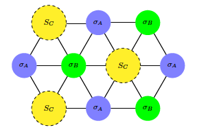
Figure 1: (Colour online) Schematic representation of the mixed spin-1/2 and 1 on a triangular lattice which consists of three interpenetrating sublattices $A$, $B$, and $C$. The small and large circles denote the spins-1/2 ($\sigma_{A}$, $\sigma_{B}$) and spin-1 ($S_{C}$) sites, respectively. The full-straight lines represent the nearest neighbor interaction $J<0$ and the dashed line denotes the existence of the random anisotropy.

In order to study the behaviour of the thermodynamic quantities of a mixed-spin Ising system on the triangular lattice with random anisotropy, we define the following Hamiltonian model,

$$\mathcal{H}=-J\Bigl{(}\sum_{i\in A,j\in B}\sigma_{i}\sigma_{j}+\sum_{i\in A,k\in C}\sigma_{i}S_{k}+\sum_{j\in B,k\in C}\sigma_{j}S_{k}\Bigr{)}-\sum_{k\in C}D_{k}S_{k}^{2},$$ (2.1)

where the spin variables assume the values $\sigma=\pm 1/2$, $S=\pm 1$ and 0, and the nearest-neighbor interaction is $J<0$. Here, there are three different antiferromagnetic interaction types between the nearest neighbor spins, such as $\sigma_{B}\leftrightarrow\sigma_{A}$, $\sigma_{B}\leftrightarrow S_{C}$ and $\sigma_{A}\leftrightarrow S_{C}$ (see figure 1). They are distributed on three interpenetrating sublattices $A$, $B$, and $C$. The random anisotropy $D_{k}$ in the last term of equation (2.1) satisfies the following probability distribution:

$$P(D_{k})=p\delta(D_{k})+(1-p)\delta(D_{k}-D),$$ (2.2)

where the term $p\delta(D_{k})$ of the equation (2.2) indicates that a percentage $p$ of spins on the sublattice $C$ is free of action of random anisotropy, whereas the term $(1-p)\delta(D_{k}-D)$ indicates a percentage ($1-p$) of spins on the sublattice $C$ under the action of a random anisotropy.

In this work, the magnetic properties of the system are studied using Monte Carlo simulations. In our simulations, we used linear lattice sizes $L$ in the range of $L=48$ ($N=2304$ sites) to 105 ($N=11025$ sites), and where $N=L^{2}$ is the number of lattice sites. These lattices consist of three interpenetrating sublattices with periodic boundary conditions. The initial states of the system were prepared randomly and updated by the Metropolis algorithm [47]. We used $10$ independent samples for any lattice size and $3.5\times 10^{6}$ MCs (Monte Carlo steps) for the calculation of average values of thermodynamic quantities of interest after discarding $1.5\times 10^{6}$ MCs for thermalization.

We calculated the sublattice magnetizations per site $m_{A}$, $m_{B}$, and $m_{C}$ defined as

$$m_{A(B)}=\frac{3}{L^{2}}\Bigl{[}\Bigl{\langle}\Bigl{|}\sum_{i\in A(B)}\sigma_{i}\Bigr{|}\Bigr{\rangle}\Bigr{]},$$ (2.3)

and

$$m_{C}=\frac{3}{L^{2}}\Bigl{[}\Bigl{\langle}\Bigl{|}\sum_{k\in C}S_{k}\Bigr{|}\Bigr{\rangle}\Bigr{]},$$ (2.4)

where $\langle\cdots\rangle$ denotes the thermal average and $[\cdots]$ denotes the average over the sample of the system. Based on the ground-state considerations (see below), for the identified ordered phases, we additionally define the following order parameters for the entire system, which take values between 0 in the fully disordered and 1 in the fully ordered phase. Thus, we need to introduce two other order parameters (staggered magnetization per site), $m_{s1}$ and $m_{s2}$, given by

$$m_{s1}=\frac{1}{L^{2}}\Bigl{[}\Bigl{\langle}\Bigl{|}\sum_{k\in C}S_{k}-2\sum_{i\in A}\sigma_{i}-2\sum_{j\in B}\sigma_{j}\Bigr{|}\Bigr{\rangle}\Bigr{]},$$ (2.5)

and

$$m_{s2}=\frac{3}{L^{2}}\Bigl{[}\Bigl{\langle}\Bigl{|}\sum_{i\in A}\sigma_{i}-\sum_{j\in B}\sigma_{j}\Bigr{|}\Bigr{\rangle}\Bigr{]}.$$ (2.6)

Further, to find all the critical points, we used the position peak of the specific heat per site, given by

$$c_{L}=\frac{[\langle E^{2}\rangle]-[\langle E\rangle]^{2}}{k_{\text{B}}T^{2}L^{2}},$$ (2.7)

where $k_{\text{B}}$ is the Boltzmann constant, $E$ is the total energy of the system and $L$ is the linear lattice size.

3 Results and discussions

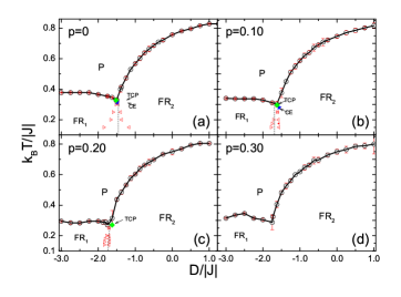
Figure 2: (Colour online) Phase diagram in the $D/\left|J\right|$ versus $k_{\text{B}}T/\left|J\right|$ plane for different values of $p$: (a) $p=0$ (special case), (b) $p=0.10$, (c) $p=0.20$, and (d) $p=0.30$. The empty circles represent the phase transition temperatures $T_{c}$ between the paramagnetic $P$ phase and the ferrimagnetic $FR_{1}$ and $FR_{2}$ phases calculated by the specific heat peaks. The empty triangles denote the hysteresis widths and the dotted lines represent an eye guide for the first-order phase transition lines. The green-diamond and blue-star dots denote the tricritical point (TCP) and the critical endpoint (CE), respectively.

Firstly, we calculated all the possible ground-states for the entire range of the anisotropy parameter $D/\left|J\right|$. We considered the lattice of the system consisting of three interpenetrating sublattices $A$, $B$, and $C$, as schematically defined in figure 1 and in the Hamiltonian, equation (2.1). Focusing on a triangular elementary unit cell consisting of the spins $\sigma_{A}$, $\sigma_{B}$, $S_{C}$, one can obtain expressions for the reduced energies per spin $E/(N\left|J\right|)$ of different spin arrangements as functions of $D/\left|J\right|$. Then, the ground-states are determined as configurations corresponding to the lowest energies for different values of $D/\left|J\right|$, the ground-state configurations and the respective energies for different ranges of the anisotropy parameter. Therefore, we defined: (i) the $FR_{1}$ phase with states ($\pm 1/2,\mp 1/2,0$) and energy $E/(N\left|J\right|)=-1/4$ for anisotropy in the range of $-\infty\leqslant D/\left|J\right|\leqslant-3/2$, (ii) the $FR_{2}$ phase with states ($\pm 1/2,\pm 1/2,\mp 1$) and energy $\frac{E}{N\left|J\right|}=-3/4-\frac{D}{3\left|J\right|}$ for anisotropy in the range of $-3/2\leqslant D/\left|J\right|\leqslant+\infty$. On the other hand, for $k_{\text{B}}T/\left|J\right|\neq 0$ besides the ordered ferrimagnetic $FR_{1}$ and $FR_{2}$ phases (similar at $k_{\text{B}}T/\left|J\right|=0$), we also have another phase, i.e., the paramagnetic $P$ phase. We can note that in the $FR_{1}$ phase, the zero means nonmagnetic states $S_{k}=0$ of spins on sublattice $C$. The critical value of the anisotropy parameter separating the respective $FR_{1}$ and $FR_{2}$ phases is given by $D_{c}/\left|J\right|=-3/2$.

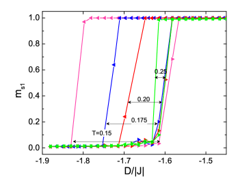
Figure 3: (Colour online) The hysteresis loops of the system, staggered magnetization $m_{s1}$ as a function of the strength of the random anisotropy $D/\left|J\right|$. The symbols $\blacktriangleright$ and $\blacktriangleleft$ indicate that $m_{S1}$ increases and decreases with strength of $D/\left|J\right|$, respectively. These loops were obtained for different values of temperatures $k_{\text{B}}T/\left|J\right|$ as indicated in the figure. Here, we used $L=66$ ($N=4356$ sites) and $p=0.10$. The error bars are within the symbol size.

Now, let us turn our attention to figure 2, where we presented the phase diagram in the $D/\left|J\right|$ versus $k_{\text{B}}T/\left|J\right|$ plane for some select values of $p\leqslant 0.3$, for instance, for $p=0$ (special case, see figure 2(a)), $p=0.10$ (figure 2(b)), $p=0.20$ (figure 2(c)), and $p=0.30$ (figure 2(d)). The results for the special case $p=0$ in figure 2(a) were obtained in a way similar to the ones obtained by Z̆ukovic̆ and Bobák [46] and we reproduced the results here. This case is related to the situation that all the spins on the sublattice $C$ are under the influence of anisotropy $D/\left|J\right|$. In this case, the topology of the phase diagram presents three different phases: the paramagnetic $P$ phase, the ferrimagnetic $FR_{1}$ phase and another ordered phase also ferrimagnetic $FR_{2}$ phase. The phase transitions between the $P-FR_{1}$ and $P-FR_{2}$ phases are continuous phase transitions (second-order phase transition). The empty circles represent the phase transition temperatures $k_{\text{B}}T_{c}/\left|J\right|$ between the phases and are estimated by the specific heat peak $c$, equation (2.7). We found $k_{\text{B}}T_{c}/\left|J\right|=0.757\pm 0.001$ for $D/\left|J\right|=0$ and it is approximately equal to the results obtained by Z̆ukovic̆. We can also observe a first-order transition line between the ordered $FR_{1}-FR_{2}$ phases at low temperature. We used the same technique that was used by Z̆ukovic̆ which consists of plotting the order parameter (in our case, the staggered magnetization $m_{s1}$, equation (2.5) increasing and decreasing as a function of $D/\left|J\right|$. Through these plots, we can observe its discontinuous character by the appearance of hysteresis loops, and when the width of the hysteresis loops increases for lower temperatures. Similar behaviour is demonstrated in figure 3 for the magnetization $m_{s1}$ and $p=0.10$, where such behaviour signals a first-order phase transition. These hysteresis loops persist for higher temperatures, but this behaviour disappears when the temperature increases and is close to the critical endpoint (CE) and the tricritical point (TCP). The highest temperatures at which we still could observe some signs of first-order phase transitions after this behaviour disappear. Thereby, we can estimate the coordinate of the CE and the TCP points. We found for the coordinate of the CE ($D_{\text{CE}}/\left|J\right|=-1.618$, $k_{\text{B}}T_{\text{CE}}/\left|J\right|=0.296$) and the TCP ($D_{\text{TCP}}/\left|J\right|=-1.520$, $k_{\text{B}}T_{\text{TCP}}/\left|J\right|=0.327$) points for the case $p=0$.

When we decrease the number of spins on the sublattice $C$ under the action of the anisotropy $D/\left|J\right|$, that is, the value of $p$ becomes greater (see figure 2(b) with $p=0.10$ (10%)), this anisotropy makes the critical temperature to decrease. Therefore, it induces the first-order transition line for smaller values of $D/\left|J\right|$ and temperature in the range of $0.3\geqslant k_{\text{B}}T/\left|J\right|\geqslant 0.2$. Here, we can see that the transition again becomes second-order for large values of $D/\left|J\right|$. In this case, the CE and the TPC points are located only in regions of lower temperatures where the coordinates are ($D_{\text{CE}}/\left|J\right|=-1.563$, $k_{\text{B}}T_{\text{CE}}/\left|J\right|=0.280$) and ($D_{\text{TCP}}/\left|J\right|=-1.625$, $k_{\text{B}}T_{\text{TCP}}/\left|J\right|=0.302$), respectively. Moreover, in figure 2(c) we can observe a decrease in the region of hysteresis loops where there is the first-order phase transition. For this case with $p=0.20$, the coordinate of the TCP is ($k_{\text{B}}D_{\text{TCP}}/\left|J\right|=-1.75$, $k_{\text{B}}T_{\text{TCP}}/\left|J\right|=0.27$). Here, due to the difficulties in the simulations, we did not obtain the coordinates of the CE point. On the other hand, for the case $p=0.30$ shown in figure 2(d), we did not find a first-order phase transition between the $FR_{1}$ and $FR_{1}$ phases using the hysteresis loop technique. We found a critical parameter $p_{c}=0.25$, where the first-order phase transition line $FR_{1}-FR_{2}$ disappears.

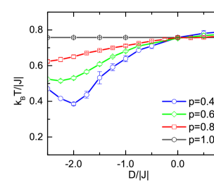
Figure 4: (Colour online) The phase diagram in the $D/\left|J\right|$ versus $k_{\text{B}}T/\left|J\right|$ plane for values of $0.4\leqslant p\leqslant 1.0$, as indicated in the figure. The full lines represent the phase transition lines between the paramagnetic $P$ and the ferrimagnetic $FR_{2}$ phases.

A behaviour hysteresis loop characteristic is shown in figure 3, where we exhibit the magnetization $m_{s1}$ as a function of an increase and decrease of the strength of the random anisotropy parameter $D/\left|J\right|$ for different values of temperatures such as $k_{\text{B}}T/\left|J\right|=0.15$, 0.175, 0.20, 0.25. When we increase the temperature, the area of the hysteresis loop decreases until the disappearance of $k_{\text{B}}T/\left|J\right|\geqslant 0.30$.

For other values of $p$ in the range of $0.40\leqslant p\leqslant 1.00$, we also illustrated in figure 4 the phase diagram in the $D/\left|J\right|$ versus $k_{\text{B}}T/\left|J\right|$ plane. The empty symbols represent the phase transition temperatures $k_{\text{B}}T_{c}/\left|J\right|$ between the paramagnetic $P$ and the ferrimagnetic $FR_{2}$ phases and they are all second-order phase transitions. All the values were estimated by the specific heat peak, equation (2.7). Another important point we want to emphasize is that for $p=1.00$ where $k_{\text{B}}T_{c}/\left|J\right|$ is independent of the anisotropy $D/\left|J\right|$.

Due to the great difficulty in simulating at low temperatures and to have a complete idea of what happens with the different phase regions in the phase diagram when we change $p$, we decided to construct a phase diagram with background colours. Thereby, we can visualize the effects of the strength of the anisotropy dilution in the phase topology of the phase diagrams. To this end, we constructed this diagram using the following definition for the parameter, $M_{d}=m_{s1}-m_{s2}$. This new parameter has a range of ($-1.0$) to (1.0) where we can assign a colour spectrum as can be shown in figure 5. When $m_{s1}\rightarrow 1.0$ and $m_{s2}\rightarrow 0$ so $M_{d}\rightarrow 1.0$, on the other hand, when $m_{s1}\rightarrow 0$ and $m_{s2}\rightarrow 1.0$ so $M_{d}\rightarrow-1.0$. Using this definition, we have presented in figure 5 an example of the phase diagram with different background colours in the $D/\left|J\right|$ versus $k_{\text{B}}T/\left|J\right|$ plane for the case $p=0$. The red colour denotes the ferrimagnetic $FR_{1}$ phase ($M_{d}\approx-1.0$), green is the ferrimagnetic $FR_{2}$ phase ($M_{d}\approx 1.0$) and blue is the paramagnetic $P$ phase ($M_{d}\approx 0$). As we can see, the dominant colours correspond to the areas of the phases as seen in figure 2(a) (case $p=0$) and which correspond to the ferrimagnetic $FR_{2}$ phase (green), the ferrimagnetic $FR_{1}$ phase (red) and the paramagnetic $P$ phase (blue). To make it clearer, we also plot the data of figure 2(a) in figure 5.

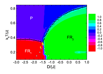
Figure 5: (Colour online) Phase diagram with different background colours in the $k_{\text{B}}T/\left|J\right|$ versus $D/\left|J\right|$ plane for the case $p=0$. The red colour is the ferrimagnetic $FR_{1}$ phase, green is the ferrimagnetic $FR_{2}$ phase, and blue is the paramagnetic $P$ phase.

Thus, in figure 6 we exhibited the phase diagram with background colours in the $k_{\text{B}}T/\left|J\right|$ versus $D/\left|J\right|$ plane for several values of $p$ in the range of $0\leqslant p\leqslant 0.35$. Here, the colours continue to be red for the ferrimagnetic $FR_{1}$ phase, green for the ferrimagnetic $FR_{2}$ phase, and blue for the paramagnetic $P$ phase. For the case $p=0$, we have the same topology as presented in figure 5 and obtained by Z̆ukovic̆ [46]. On the other hand, when $p$ increases ($p\geqslant 0.05$) we can observe that the $FR_{1}$ phase decreases more and more (see $p=0.30$ and 0.35) and then for $p\gtrapprox 0.4$ (see in figure 7) the phase diagram presents only two $P$ and $FR_{2}$ dominant phases. This case means that we have approximately $40\%$ or more spins under the influence of random anisotropy $D/\left|J\right|$.

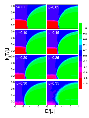
Figure 6: (Colour online) Phase diagram with different background colours in the $k_{\text{B}}T/\left|J\right|$ versus $D/\left|J\right|$ for values of $0\leqslant p\leqslant 0.35$, as indicated in the figures. The red colour is the ferrimagnetic $FR_{1}$ phase, green is the ferrimagnetic $FR_{2}$ phase, and blue is the paramagnetic $P$ phase.

Finally, in figure 7, we displayed the phase diagram which is a continuation of figure 6, but now for values of $p$ in the range of $0.4\leqslant p\leqslant 1.0$. In this case, we still have only two phases, the $P$ and $FR_{2}$ phases. When $p$ increases, the $FR_{2}$ phase grows for $D/\left|J\right|\rightarrow-\infty$. This growth starts at $p\gtrapprox 0.4$ and goes on increasing until it occupies all the region for $k_{\text{B}}T/\left|J\right|=0.757$ in the case $p=1.0$. All of these results corroborate the results shown in figure 4, i.e. We can see that the phase boundary that separates the $P$ from the $FR_{2}$ phase region coincides with the phase separation line in figure 4 for $p=1.0$.

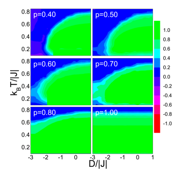
Figure 7: (Colour online) Phase diagram with different background colours in the $k_{\text{B}}T/\left|J\right|$ versus $D/\left|J\right|$ for values of $0.4\leqslant p\leqslant 1.0$, as indicated in the figures. The colour green is the ferrimagnetic $FR_{2}$ phase and blue is the paramagnetic $P$ phase.

4 Conclusions

In conclusion, we used Monte Carlo simulations to study the phase diagram of the mixed spin-1/2 and 1 Ising ferrimagnetic system with a random anisotropy on a triangular lattice with three interpenetrating sublattices $A$, $B$, and $C$. The spins on the sublattices are represented by $\sigma_{A}$, $\sigma_{B}$, $S_{C}$ with states $\pm 1/2$, $\pm 1/2$, $\pm 1$ and 0, respectively. We obtained the phase diagram at the temperature $k_{\text{B}}T/\left|J\right|$ versus the strength of the random anisotropy $D/\left|J\right|$ plane, where the anisotropy is randomly distributed on the sublattice $C$ (with spins $S_{C}$) according to the bimodal probability distribution $P(D_{k}/\left|J\right|)$. Therefore, we can conclude that the phase boundary in the phase diagram presents a topology that depends on the parameter $p$. We found a first-order transition line between the two ferrimagnetic $FR_{1}$ and $FR_{2}$ phases at lower temperatures for $p<0.25$ together with a second-order phase transition between the $FR_{1}-P$ and $FR_{2}-P$ phases. On the other hand, for $p\gtrapprox 0.4$, i.e., above $40\%$ of the sites on the sublattice $C$ are free of $D/\left|J\right|$. The phase diagram presents only second-order phase transition lines between ordered and paramagnetic $P$ phase showing that the system no longer exhibits the tricritical behaviour.

5 Acknowledgements

The authors acknowledge financial support from the Brazilian agencies CNPq and CAPES.

Ukrainian 0

[Âèïàäêîâà àíiçîòðîïiÿ ó ñèñòåìi çi çìiøàíèìè ñïiíàìè Içèíãà íà òðèêóòíié ґðàòöi] Âèïàäêîâà àíiçîòðîïiÿ ó ñèñòåìi çi çìiøàíèìè ñïiíàìè Içèíãà íà òðèêóòíié ґðàòöi [Å. Ñ. äå Ñàíòàíà, À. Ñ. äå Àððóäà, Ì. Ãîäîé] Å. Ñ. äå Ñàíòàíà, À. Ñ. äå Àððóäà, Ì. Ãîäîé

             
Iíñòèòóò ôiçèêè, Ôåäåðàëüíèé óíiâåðñèòåò Ìàòó-Ãðîñó, 78060-900, Êóÿáà, Ìàòó-Ãðîñó, Áðàçèëiÿ

References

- [1] Mallah T., Thiebaut S., Verdaguer M., Veillet P., Science, 1993, 262, 1554, doi:10.1126/science.262.5139.1554.
-
[2]
Okawa H., Matsumoto N., Tamaki H., Ohba M., Mol. Cryst. Liq. Cryst. Lett., 1993, 233, 257,
doi:10.1080/10587259308054965. - [3] Mathoniere C., Nutall C. J., Carling S. G., Day P., Inorg. Chem., 1996, 35, 1201, doi:10.1021/ic950703v.
- [4] Kahn O., Molecular Magnetism, VCH-Verlag, Weinheim, New York, 1993.
- [5] Kaneyoshi T., Nakamura Y., J. Phys.: Condens. Matter, 1998, 10, 3003, doi:10.1088/0953-8984/10/13/017.
-
[6]
Kaneyoshi T., Nakamura Y., Shin S., J. Phys.:Condens. Matter, 1998, 10, 7025,
doi:10.1088/0953-8984/10/31/018. -
[7]
Verona de Resende H. F., Sá Barreto F. C., Plascak J. A., Physica A, 1988, 149, 606,
doi:10.1016/0378-4371(88)90121-5. - [8] Goncalves L. L., Phys. Scr., 1985, 32, 248, doi:10.1088/0031-8949/32/3/012.
- [9] Lipowski A., Horiguchi T., J. Phys. A: Math. Gen., 1995, 28, L261, doi:10.1088/0305-4470/28/9/003.
- [10] Jas̆c̆ur M., Physica A, 1998, 252, 217, doi:10.1016/S0378-4371(97)00584-0.
- [11] Dakhama A., Physica A, 1998, 252, 225, doi:10.1016/S0378-4371(97)00583-9.
-
[12]
Souza I. J., de Arruda P. H. Z., Godoy M., Craco L.,
de Arruda A. S., Physica A, 2016, 444,
589, doi:10.1016/j.physa.2015.10.089. -
[13]
Da Cruz Filho J. S., Tunes T. M., Godoy M.,
de Arruda A. S., Physica A, 2016, 450, 180,
doi:10.1016/j.physa.2015.12.096. - [14] Da Cruz Filho J. S., Godoy M., de Arruda A. S., Physica A, 2013, 392, 6247, doi:10.1016/j.physa.2015.12.096.
- [15] Reyes J. A., de La Espriella N., Buendía G. M., Phys. Status Solidi B, 2015, 10, 252, doi:10.1002/pssb.201552110.
-
[16]
De La Espriella N., Mercado C. A., Madera J. C.,
J. Magn. Magn. Mater., 2016, 401, 22,
doi:10.1016/j.jmmm.2015.09.083. -
[17]
Abubrig O. F., Horváth D., Bobák A., Jas̆c̆ur M.,
Physica A, 2001, 296, 437,
doi:10.1016/S0378-4371(01)00176-5. - [18] Kaneyoshi T., Physica A, 1988, 153, 556, doi:10.1016/0378-4371(88)90240-3.
- [19] Kaneyoshi T., J. Magn. Magn. Mater., 1990, 92, 59, doi:10.1016/0304-8853(90)90679-K.
-
[20]
Benyoussef A., El Kenz A., Kaneyoshi T., J. Magn. Magn. Mater., 1994, 131, 173,
doi:10.1016/0304-8853(94)90025-6. -
[21]
Benyoussef A., El Kenz A., Kaneyoshi T., J. Magn. Magn. Mater., 1994, 131, 179,
doi:10.1016/0304-8853(94)90026-4. - [22] Quadros S. G. A., Salinas S. R., Physica A, 1994, 206, 479, doi:10.1016/0378-4371(94)90319-0.
- [23] Zhang G. M., Yang Ch. Z., Phys. Rev. B, 1993, 48, 9452, doi:10.1103/PhysRevB.48.9452.
- [24] Buendia G. M., Liendo J. A., J. Phys.: Condens. Matter, 1997, 9, 5439, doi:10.1088/0953-8984/9/25/011.
- [25] Godoy M., Figueiredo W., Phys. Rev. E, 2000, 61, 218, doi:10.1103/PhysRevE.61.218.
-
[26]
Pereira J. R. V., Tunes T. M., de Arruda A. S.,
Godoy M., Physica A, 2018, 500, 265,
doi:10.1016/j.physa.2018.02.085. -
[27]
Da Silva D. C., de Arruda A. S., Godoy M., Int.
J. Mod. Phys. C, 2020, 31, No. 9, 2050124,
doi:10.1142/S0129183120501247. - [28] Kaneyoshi T., Chen J. C., J. Magn. Magn. Mater., 1991, 98, 201, doi:10.1016/0304-8853(91)90444-F.
- [29] Kaneyoshi T., J. Phys. Soc. Jpn., 1987, 56, 2675, doi:10.1143/JPSJ.56.2675.
- [30] Bobák A., Jurc̆is̆ M., Physica A, 1997, 240, 647, doi:10.1016/S0378-4371(97)00044-7.
- [31] Oitmaa J., Enting I. G., J. Phys.: Condens. Matter, 2006, 18, 10931, doi:10.1088/0953-8984/18/48/020.
- [32] Selke W., Oitmaa J., J. Phys.: Condens. Matter, 2010, 22, 076004, doi:10.1088/0953-8984/22/7/076004.
- [33] Figueiredo W., Godoy M., Leite V. S., Braz. J. Phys., 2004, 34, No. 2A, doi:10.1590/S0103-97332004000300010.
- [34] Leite V. S., Godoy M., Figueiredo W., Phys. Rev. B, 2005, 71, 094427, doi:10.1103/PhysRevB.71.094427.
- [35] Z̆ukovic̆ M., Bobák A., Physica A, 2015, 436, 509, doi:10.1016/j.physa.2015.05.077.
-
[36]
Ertas M., Kocakaplan Y., Kantar E., J. Magn. Magn. Mater., 2015, 386, No. 1–7,
doi:10.1016/j.jmmm.2015.03.058. -
[37]
Strečka J., Rebic M., Rojas O., de Souza S. M.,
J. Magn. Magn. Mater., 2019, 469, 655,
doi:10.1016/j.physleta.2019.05.017. - [38] Zad H. A., Ananikian N., J. Phys.: Condens. Matter, 2018, 30, 165403, doi:10.1088/1361-648X/ab3136.
- [39] Z̆ukovic̆ M., Bobák A., Phys. Rev. E, 2013, 87, 032121, doi:10.1103/PhysRevE.87.032121.
- [40] Theodorakis P. E., Fytas N. G., Phys. Rev. E, 2012, 86, 011140, doi:10.1103/PhysRevE.86.011140.
- [41] Kantar E., Ertas M., Phase Transitions, 2018, 91, No. 4, 370–381, doi:10.1080/01411594.2017.1402897.
- [42] Ertas M., Kantar E., J. Supercond. Novel Magn., 2015, 28, 3037–3044, doi:10.1007/s10948-015-3134-2.
- [43] Ertas M., Kantar E., Kocakaplan Y., Keskin M., Physica A, 2016, 444, 732, doi:10.1016/j.physa.2015.10.069.
- [44] Kudasov Y. B., Phys. Rev. Lett., 2006, 96, 027212, doi:10.1103/PhysRevLett.96.027212.
-
[45]
Soto R., Martinez G., Baibich M. N., Florez J. M.,
Vargas P., Phys. Rev. B, 2009, 79, 184422,
doi:10.1103/PhysRevB.79.184422. - [46] Z̆ukovic̆ M., Bobák A., Phys. Rev. E, 2015, 91, 052138, doi:10.1103/PhysRevE.91.052138.
- [47] Metropolis N., Rosenbluth A., Rosenbluth M., Teller A., Teller E., J. Chem. Phys., 1953, 21, 1087, doi:10.1063/1.1699114.
Ukrainian \adddialect\l@ukrainian0 \l@ukrainian