Stochastic Modified Equations and Dynamics of Dropout Algorithm

Abstract

Dropout is a widely utilized regularization technique in the training of neural networks, nevertheless, its underlying mechanism and its impact on achieving good generalization abilities remain poorly understood. In this work, we derive the stochastic modified equations for analyzing the dynamics of dropout, where its discrete iteration process is approximated by a class of stochastic differential equations. In order to investigate the underlying mechanism by which dropout facilitates the identification of flatter minima, we study the noise structure of the derived stochastic modified equation for dropout. By drawing upon the structural resemblance between the Hessian and covariance through several intuitive approximations, we empirically demonstrate the universal presence of the inverse variance-flatness relation and the Hessian-variance relation, throughout the training process of dropout. These theoretical and empirical findings make a substantial contribution to our understanding of the inherent tendency of dropout to locate flatter minima.

1 Introduction

Dropout is used with gradient-descent-based algorithms for training neural networks (NNs) (Hinton et al., 2012; Srivastava et al., 2014), which obtains the state-of-the-art test performance in deep learning (Tan and Le, 2019; Helmbold and Long, 2015). The key idea behind dropout is to randomly remove a subset of neurons during the training process, specifically, the output of each neuron is multiplied with a random variable that takes the value $1/p$ with probability $p$ and zero otherwise. This random variable is independently sampled at each feedforward operation. In contrast to the widespread use and empirical success of dropout, the mechanism by which it helps generalization in deep learning remains an ongoing area of research.

The noise structure introduced by stochastic algorithms is important for understanding their training behaviors. A series of recent works reveal that the noise structure inherent in stochastic gradient descent (SGD) plays a crucial role in facilitating the exploration of flatter solutions (Keskar et al., 2016; Feng and Tu, 2021; Zhu et al., 2018). Analogously, training with dropout introduces some noise with a specific type of architecture, acting as an implicit regularizer that facilitates better generalization abilities (Hinton et al., 2012; Srivastava et al., 2014; Wei et al., 2020; Zhang and Xu, 2022; Zhu et al., 2018).

In this paper, we first employ the framework of stochastic modified equations (SMEs) (Li et al., 2017) to approximate in distribution the training dynamics of the dropout algorithm applied to two-layer NNs. By employing this approach, we are able to quantify the leading order dynamics of the dropout algorithm and its variants in a precise manner. Additionally, we calculate the covariance structure of the noise generated by the stochasticity incorporated in dropout. We then utilize the covariance structure to understand why NNs trained by dropout have the tendency to possess better generalization abilities from the perspective of flatness (Keskar et al., 2016; Neyshabur et al., 2017).

We hypothesize that the flatness-improving ability of dropout noise is attributed to its alignment with the structure of the loss landscape, based on the similarity between the explicit forms of the Hessian and the dropout covariance under intuitive approximations. To investigate this hypothesis, we conduct empirical studies using three different approaches (shown respectively in Fig. 1, Fig. 2(a, b), and Fig. 2(c, d)) to assess the similarity between the flatness of the loss landscape and the noise structure induced by dropout at the obtained minima, and all of them consistently demonstrate two important relationships: i) Inverse variance-flatness relation: The noise is larger at the sharper direction of the loss landscape; ii) Hessian-variance alignment relation: The Hessian of the loss landscape at the found minima aligns with the noise covariance matrix. These two relations are compatible with each other in that they collectively contribute to the ability of the training algorithm to effectively identify flatter minima. Our experiments are conducted on several representative datasets, i.e., MNIST (LeCun et al., 1998), CIFAR-100 (Krizhevsky et al., 2009) and Multi30k (Elliott et al., 2016), and also on distinct NN structures, i.e., fully-connected neural networks (FNNs), ResNet-20 (He et al., 2016) and transformer (Vaswani et al., 2017) to demonstrate the universality of our findings.

2 Related works

A flurry of recent works aims to shed light on the regularization effect conferred by dropout. Wager et al. (2013) show that dropout performs a form of adaptive regularization in the context of linear regression and logistic problems. McAllester (2013) propose a PAC-Bayesian bound, whereas Wan et al. (2013); Mou et al. (2018) derive some Rademacher-complexity-type error bounds specifically tailored for dropout. Mianjy and Arora (2020) demonstrate that dropout training with logistic loss achieves $\varepsilon$-suboptimality in test error within $O(1/\varepsilon)$ iterations. Finally, Zhang and Xu (2022) establish that dropout enhances the flatness of the loss landscape and facilitates condensation through an additional regularization term endowed by dropout.

Continuous formulations have been extensively utilized to study the dynamical behavior of stochastic algorithms. Li et al. (2017, 2019) present an entirely rigorous and self-contained mathematical formulation of the SME framework that applies to a wide class of stochastic algorithms. Furthermore, Feng et al. (2017) adopt a semigroup approach to investigate the dynamics of SGD and online PCA. Malladi et al. (2022) derive the SME approximations for the adaptive stochastic algorithms including RMSprop and Adam, additionally, they provide efficient experimental verification of the validity of square root scaling rules arising from the SMEs.

One noteworthy observation is the association between the flatness of minima and improved generalization ability (Li et al., 2017; Jastrzebski et al., 2017, 2018). Specifically, SGD is shown to preferentially select flat minima, especially under conditions of large learning rates and small batch sizes (Jastrzebski et al., 2017, 2018; Wu et al., 2018). Papyan (2018, 2019) attribute such enhancement of flatness by SGD to the similarity between covariance of the noise and Hessian of the loss function. Furthermore, Feng and Tu (2021) reveal an inverse variance–flatness relation within the dynamics of SGD. Additionally, Zhu et al. (2018); Wu et al. (2022) unveil the Hessian-variance alignment property of SGD noise, shedding light on the role of SGD in escaping from sharper minima and locating flatter minima.

3 Preliminary

In this section, we present the notations and definitions that are utilized in our theoretical analysis. We remark that our experimental settings are more general than the counterparts in the theoretical analysis.

3.1 Notations

We set a special vector $(1,1,1,\dots,1)^{\intercal}$ by $\bm{1}:=(1,1,1,\dots,1)^{\intercal}$ whose dimension varies. We set $n$ for the number of input samples and $m$ for the width of the NN. We let $[n]=\{1,2,\ldots,n\}$. We denote $\otimes$ as the Kronecker tensor product, and $\left<\cdot,\cdot\right>$ for standard inner product between two vectors. We denote vector $L^{2}$ norm as $\left\lVert\cdot\right\rVert_{2}$, vector or function $L_{\infty}$ norm as $\left\lVert\cdot\right\rVert_{\infty}$. Finally, we denote the set of continuous functions $f(\cdot):\mathbb{R}^{D}\to\mathbb{R}$ possessing continuous derivatives of order up to and including $r$ by $\mathcal{C}^{r}(\mathbb{R}^{D})$, the space of bounded measurable functions by $\mathcal{B}_{b}(\mathbb{R}^{D})$, and the space of bounded continuous functions by $\mathcal{C}_{b}(\mathbb{R}^{D})$.

3.2 Two-layer neural networks and loss function

We consider the empirical risk minimization problem given by the quadratic loss:

$$\min_{\bm{\theta}}R_{\mathcal{S}}(\bm{\theta})=\frac{1}{2n}\sum_{i=1}^{n}\left({f_{\bm{\theta}}(\bm{x}_{i})-y_{i}}\right)^{2},$$ (1)

where $\mathcal{S}:=\{(\bm{x}_{i},y_{i})\}_{i=1}^{n}$ is the training sample, $f_{\bm{\theta}}(\bm{x})$ is the prediction function, $\bm{\theta}$ are the parameters, and their dependence is modeled by a two-layer NN with $m$ hidden neurons

$$f_{\bm{\theta}}(\bm{x}):=\sum_{r=1}^{m}a_{r}\sigma(\bm{w}_{r}^{\intercal}\bm{x}),$$ (2)

where $\bm{x}\in\mathbb{R}^{d}$, $\bm{\theta}=\mathrm{vec}(\bm{\theta}_{a},\bm{\theta}_{\bm{w}})\in\mathbb{R}^{D}$, where $D:=m(d+1)$ throughout this paper. We remark that $\bm{\theta}$ is the set of parameters with $\bm{\theta}_{a}=\mathrm{vec}(\{a_{r}\}_{r=1}^{m})$, $\bm{\theta}_{\bm{w}}=\mathrm{vec}(\{\bm{w}_{r}\}_{r=1}^{m})$, and $\sigma(\cdot)$ is the activation function. More precisely, $\bm{\theta}=\mathrm{vec}(\{\bm{q}_{r}\}_{r=1}^{m})$, where for each $r\in[m]$, $\bm{q}_{r}:=(a_{r},\bm{w}_{r}^{\intercal})^{\intercal}$, and the bias term $b_{r}$ can be incorporated by expanding $\bm{x}$ and $\bm{w}_{r}$ to $(\bm{x}^{\intercal},1)^{\intercal}$ and $\left(\bm{w}_{r}^{\intercal},b_{r}\right)^{\intercal}$.

3.3 Dropout

Given fixed learning rate $\varepsilon>0$, then at the $N$-th iteration where $t_{N}:=N\varepsilon$, a scaling vector $\bm{\eta}_{N}\in\mathbb{R}^{m}$ is sampled with independent random coordinates: For each $k\in[m]$,

$$(\bm{\eta}_{N})_{k}=\begin{cases}\frac{1}{p}&\text{ with probability }p,\\ 0&\text{ with probability }1-p,\end{cases}$$ (3)

and we observe that $\{\bm{\eta}_{N}\}_{N\geq 1}$ is an i.i.d. Bernoulli sequence with $\mathbb{E}\bm{\eta}_{N}=\bm{1}$. With slight abuse of notations, the $\sigma$-fields $\mathcal{F}_{N}:=\left\{\sigma(\bm{\eta}_{1},\bm{\eta}_{2},\cdots\bm{\eta}_{N})\right\}$ forms a natural filtration. We then apply dropout to the two-layer NNs by computing

$$f_{\bm{\theta}}(\bm{x};\bm{\eta}):=\sum_{r=1}^{m}(\bm{\eta})_{r}a_{r}\sigma(\bm{w}_{r}^{\intercal}\bm{x}),$$ (4)

and we denote the empirical risk associated with dropout by

$$R_{S}^{\mathrm{drop}}\left(\bm{\theta};\bm{\eta}\right) :=\frac{1}{2n}\sum_{i=1}^{n}\left(f_{\bm{\theta}}(\bm{x}_{i};\bm{\eta})-y_{i}\right)^{2}=\frac{1}{2n}\sum_{i=1}^{n}\left(\sum_{r=1}^{m}(\bm{\eta})_{r}a_{r}\sigma(\bm{w}_{r}^{\intercal}\bm{x}_{i})-y_{i}\right)^{2}.$$ (5)

We observe that the parameters at the $N$-th step are updated as follows:

$$\bm{\theta}_{N}=\bm{\theta}_{N-1}-\varepsilon\nabla_{\bm{\theta}}R_{S}^{\mathrm{drop}}\left(\bm{\theta}_{N-1};\bm{\eta}_{N}\right),$$ (6)

where $\bm{\theta}_{0}:=\bm{\theta}(0)$. Finally, we denote hereafter that for all $i\in[n]$,

$$e_{i}^{N}:=e_{i}(\bm{\theta}_{N-1};\bm{\eta}_{N}):=f_{\bm{\theta}_{N-1}}(\bm{x}_{i};\bm{\eta}_{N})-y_{i}.$$

4 Stochastic modified equations for dropout

In this section, we approximate the iterative process of dropout (6) in the weak sense (Definition 1).

4.1 Modified loss

As the dropout iteration (6) can be written into

$$\bm{\theta}_{N}-\bm{\theta}_{N-1} =-\varepsilon\nabla_{\bm{\theta}}R_{S}^{\mathrm{drop}}\left(\bm{\theta}_{N-1};\bm{\eta}_{N}\right)=-\frac{\varepsilon}{n}\sum_{i=1}^{n}e_{i}^{N}\nabla_{\bm{\theta}}e_{i}^{N}.$$

Since $\bm{\theta}=\mathrm{vec}(\{\bm{q}_{r}\}_{r=1}^{m})=\mathrm{vec}\left(\{(a_{r},\bm{w}_{r})\}_{r=1}^{m}\right)$, then given $\bm{\theta}_{N-1}$, for each $k\in[m]$, the expectation of the increment restricted to $\bm{q}_{k}$ reads

$$\mathbb{E}_{\bm{\theta}_{N-1}}\left[\sum_{i=1}^{n}e_{i}^{N}\nabla_{\bm{q}_{k}}e_{i}^{N}\right]=\mathbb{E}_{\bm{\theta}_{N-1}}\left[\sum_{i=1}^{n}e_{i}^{N}(\bm{\eta}_{N})_{k}\nabla_{\bm{q}_{k}}\left(a_{k}\sigma(\bm{w}_{k}^{\intercal}\bm{x}_{i})\right)\right]$$

$$= \sum_{i=1}^{n}e_{i}\nabla_{\bm{q}_{k}}\left(a_{k}\sigma(\bm{w}_{k}^{\intercal}\bm{x}_{i})\right)+\frac{1-p}{p}\sum_{i=1}^{n}a_{k}\sigma(\bm{w}_{k}^{\intercal}\bm{x}_{i})\nabla_{\bm{q}_{k}}\left(a_{k}\sigma(\bm{w}_{k}^{\intercal}\bm{x}_{i})\right),$$

where we denote for simplicity that $e_{i}:=e_{i}(\bm{\theta}):=\sum_{r=1}^{m}a_{r}\sigma(\bm{w}_{r}^{\intercal}\bm{x}_{i})-y_{i},$ and compared with $e_{i}^{N}$, $e_{i}$ does not depend on the random variable $\bm{\eta}_{N}$. Hence, the modified loss $L_{S}(\cdot):\mathbb{R}^{D}\to\mathbb{R}$ for dropout can be defined as:

$$L_{S}(\bm{\theta}) :=\frac{1}{2n}\sum_{i=1}^{n}e_{i}^{2}+\frac{1-p}{2np}\sum_{i=1}^{n}\sum_{r=1}^{m}a_{r}^{2}\sigma(\bm{w}_{r}^{\intercal}\bm{x}_{i})^{2},$$ (7)

in that as $\bm{\theta}_{N-1}$ is given, by taking conditional expectation, its increment reads

$$\bm{\theta}_{N}-\bm{\theta}_{N-1} =-\varepsilon\mathbb{E}_{\bm{\theta}_{N-1}}\left[\nabla_{\bm{\theta}}R_{S}^{\mathrm{drop}}\left(\bm{\theta}_{N-1};\bm{\eta}_{N}\right)\right]=-\varepsilon\nabla_{\bm{\theta}}L_{S}(\bm{\theta})\big{|}_{\bm{\theta}=\bm{\theta}_{N-1}},$$

then in the sense of expectations, $\{\bm{\theta}_{N}\}_{N\geq 0}$ follows close to the gradient descent (GD) trajectory of $L_{S}(\bm{\theta})$ with fixed learning rate $\varepsilon$.

4.2 Stochastic modified equations

Firstly, from the results in Section 4.1, we observe that given $\bm{\theta}_{N-1}$,

$$\bm{\theta}_{N}-\bm{\theta}_{N-1}=-\varepsilon\nabla_{\bm{\theta}}L_{S}(\bm{\theta})\big{|}_{\bm{\theta}=\bm{\theta}_{N-1}}+\sqrt{\varepsilon}\bm{V}(\bm{\theta}_{N-1}),$$ (8)

where $L_{S}(\cdot):\mathbb{R}^{D}\to\mathbb{R}$ is the modified loss defined in (7), and $\bm{V}(\cdot):\mathbb{R}^{D}\to\mathbb{R}^{D}$ is a $D$-dimensional random vector, and when given $\bm{\theta}_{N-1}$, $\bm{V}(\bm{\theta}_{N-1})$ has mean $\bm{0}$ and covariance $\varepsilon\bm{\Sigma}(\bm{\theta}_{N-1})$, where $\bm{\Sigma}(\cdot):\mathbb{R}^{D}\to\mathbb{R}^{D\times{D}}$, whose expression is deferred to Section 5.1.

Consider the stochastic differential equation (SDE),

$$\mathrm{d}\bm{\Theta}_{t}=\bm{b}\left(\bm{\Theta}_{t}\right)\mathrm{d}t+\bm{\sigma}\left(\bm{\Theta}_{t}\right)\mathrm{d}\bm{W}_{t},\quad\bm{\Theta}_{0}=\bm{\Theta}(0),$$ (9)

where $\bm{W}_{t}$ is a standard $D$-dimensional Brownian motion, and its Euler–Maruyama discretization with step size $\varepsilon>0$ at the $N$-th step reads

$$\bm{\Theta}_{\varepsilon N}=\bm{\Theta}_{\varepsilon(N-1)}+\varepsilon\bm{b}\left(\bm{\Theta}_{\varepsilon(N-1)}\right)+\sqrt{\varepsilon}\bm{\sigma}\left(\bm{\Theta}_{\varepsilon(N-1)}\right)\bm{Z}_{N},$$

where $\bm{Z}_{N}\sim\mathcal{N}(\bm{0},\bm{I}_{D})$ and $\bm{\Theta}_{0}=\bm{\Theta}(0)$. Thus, if we set

$$\bm{b}\left(\bm{\Theta}\right) :=-\nabla_{\bm{\Theta}}L_{S}(\bm{\Theta}),$$ (10)

$$\bm{\sigma}\left(\bm{\Theta}\right) :=\sqrt{\varepsilon}\left(\bm{\Sigma}\left(\bm{\Theta}\right)\right)^{\frac{1}{2}},$$

$$\bm{\Theta}_{0} :=\bm{\theta}_{0},$$

then we would expect (9) to be a ‘good’ approximation of (8) with time identification $t=\varepsilon N$. Based on the previous work (Li et al., 2017), we use approximations in the weak sense (Kloeden and Platen, 2011, Section 9.7) since the path of dropout and the corresponding SDE are driven by noises sampled in different spaces.

To compare different discrete time approximations, we need to take the rate of weak convergence into consideration, and we also need to choose an appropriate class of functions as the space of test functions. We introduce the following set of smooth functions:

$$\mathcal{C}_{b}^{M}\left(\mathbb{R}^{D}\right)=\left\{f\in\mathcal{C}^{M}\left(\mathbb{R}^{D}\right)\Bigg{|}\left\lVert f\right\rVert_{\mathcal{C}^{M}}:=\sum_{|\beta|\leq M}\left\lVert\mathrm{D}^{\beta}f\right\rVert_{\infty}<\infty\right\},$$ (11)

where $\mathrm{D}$ is the usual differential operator. We remark that $\mathcal{C}_{b}^{M}(\mathbb{R}^{D})$ is a subset of $\mathcal{G}(\mathbb{R}^{D})$, the class of functions with polynomial growth, which is chosen to be the space of test functions in previous works (Li et al., 2017; Kloeden and Platen, 2011; Malladi et al., 2022). Before we proceed to the definition of weak approximation, to ensure the rigor and validity of our analysis, we assume that

Assumption 1.

There exists $T^{\ast}>0$, such that for any $t\in\left[0,T^{\ast}\right]$, there exists a unique $t$-continuous solution $\bm{\Theta}_{t}$ to SDE (9). Furthermore, for each $l\in[3]$, there exists $C(T^{\ast},\bm{\Theta}_{0})>0$, such that

$$\sup_{{0}\leq s\leq T^{\ast}}\mathbb{E}\left(\left\lVert\bm{\Theta}_{s}(\cdot)\right\rVert_{2}^{2l}\right)\leq C(T^{\ast},\bm{\Theta}_{0}).$$ (12)

Moreover, for the dropout iterations (6), let $0<\varepsilon<1$, $T>0$ and set $N_{T,\varepsilon}:=\lfloor\frac{T}{\varepsilon}\rfloor$. There exists $\varepsilon_{0}>0$, such that given any learning rate $\varepsilon\leq\varepsilon_{0}$, then for all $N\in[0:N_{T^{\ast},\varepsilon}]$ and for each $l\in[3]$, there exists $C(T^{\ast},\bm{\theta}_{0},\varepsilon_{0})>0$, such that

$$\sup_{{0}\leq N\leq[N_{T^{\ast},\varepsilon}]}\mathbb{E}\left(\left\lVert\bm{\theta}_{N}\right\rVert_{2}^{2l}\right)\leq C(T^{\ast},\bm{\theta}_{0},\varepsilon_{0}).$$ (13)

We remark that if $\mathcal{G}(\mathbb{R}^{D})$ is chosen to be the test functions in Li et al. (2019), then similar relations to (12) and (13) shall be imposed, except that in our cases, we only require the second, fourth and sixth moments to be uniformly bounded, while in their cases, all $2l$-moments are required for $l\geq 1$.

Definition 1.

The SDE (9) is an order $\alpha$ weak approximation to the dropout (6), if for every $g\in\mathcal{C}_{b}^{M}\left(\mathbb{R}^{D}\right)$, there exists $C>0$ and $\varepsilon_{0}>0$, such that given any $\varepsilon\leq\varepsilon_{0}$ and $T\leq T^{\ast}$, then for all $N\in[N_{T,\varepsilon}]$,

$$\left\lvert\mathbb{E}g(\bm{\Theta}_{\varepsilon N})-\mathbb{E}g(\bm{\theta}_{N})\right\rvert\leq C(T^{\ast},g,\varepsilon_{0})\varepsilon^{\alpha}.$$ (14)

We now state informally our approximation theorem.

Theorem 1*.

Fix time $T\leq T^{\ast}$ and learning rate $\varepsilon>0$, then if we choose

$$\bm{b}(\bm{\Theta}) =-\nabla_{\bm{\Theta}}L_{S}(\bm{\Theta}),$$

$$\bm{\sigma}(\bm{\Theta}) =\sqrt{\varepsilon}\left(\bm{\Sigma}\left(\bm{\Theta}\right)\right)^{\frac{1}{2}},$$

then for all $t\in[0,T]$, the stochastic processes $\bm{\Theta}_{t}$ satisfying

$$\mathrm{d}\bm{\Theta}_{t}=\bm{b}\left(\bm{\Theta}_{t}\right)\mathrm{d}t+\bm{\sigma}\left(\bm{\Theta}_{t}\right)\mathrm{d}\bm{W}_{t},$$

is an order-$1$ approximation of dropout (6). If we choose instead

$$\bm{b}(\bm{\Theta}) =-\nabla_{\bm{\Theta}}\left(L_{S}(\bm{\Theta})+\frac{\varepsilon}{4}\left\lVert\nabla_{\bm{\Theta}}L_{S}(\bm{\Theta})\right\rVert_{2}^{2}\right),$$

$$\bm{\sigma}(\bm{\Theta}) =\sqrt{\varepsilon}\left(\bm{\Sigma}\left(\bm{\Theta}\right)\right)^{\frac{1}{2}},$$

then $\bm{\Theta}_{t}$ is an order-$2$ approximation.

It is noteworthy that our findings reproduce the explicit regularization effect attributed to dropout (Wei et al., 2020; Zhang and Xu, 2022). This regularization effect modifies the expected training objective from $R_{\mathcal{S}}(\theta)$ to $L_{\mathcal{S}}(\theta)$. The regularization effect stems from the stochasticity of dropout. Unlike SGD, where the noise arises from the stochasticity involved in the selection of training samples, dropout introduces noise through the stochastic removal of parameters. In the sequel, we focus on how such stochasticity exerts an impact on our learning results.

5 The effect of the noise structure on flatness

We begin this section by examining the expression of the noise structure arising from dropout.

5.1 Explicit form of the dropout noise structure

In this subsection, we present the expression for $\bm{\Sigma}$. Once again, as $\bm{\theta}=\mathrm{vec}(\{\bm{q}_{r}\}_{r=1}^{m})=\mathrm{vec}\left(\{(a_{r},\bm{w}_{r})\}_{r=1}^{m}\right)$, then covariance of $\nabla_{\bm{\theta}}R_{S}^{\mathrm{drop}}\left(\bm{\theta}_{N-1};\bm{\eta}_{N}\right)$ equals to $\bm{\Sigma}(\bm{\theta}_{N-1})$. We denote

$$\bm{\Sigma}_{kr}(\bm{\theta}_{N-1}):=\mathrm{Cov}\left(\nabla_{\bm{q}_{k}}R_{S}^{\mathrm{drop}}\left(\bm{\theta}_{N-1};\bm{\eta}_{N}\right),\nabla_{\bm{q}_{r}}R_{S}^{\mathrm{drop}}\left(\bm{\theta}_{N-1};\bm{\eta}_{N}\right)\right),$$

then

$$\bm{\Sigma}=\left[\begin{array}[]{cccc}\bm{\Sigma}_{11}&\bm{\Sigma}_{12}&\cdots&\bm{\Sigma}_{1m}\\ \bm{\Sigma}_{21}&\bm{\Sigma}_{22}&\cdots&\bm{\Sigma}_{2m}\\ \vdots&\vdots&\vdots&\vdots\\ \bm{\Sigma}_{m1}&\bm{\Sigma}_{m2}&\cdots&\bm{\Sigma}_{mm}\end{array}\right].$$

For each $k\in[m]$, we obtain that

$$\bm{\Sigma}_{kk}(\bm{\theta}_{N-1})=\mathrm{Cov}\left(\nabla_{\bm{q}_{k}}R_{S}^{\mathrm{drop}}\left(\bm{\theta}_{N-1};\bm{\eta}_{N}\right),\nabla_{\bm{q}_{k}}R_{S}^{\mathrm{drop}}\left(\bm{\theta}_{N-1};\bm{\eta}_{N}\right)\right)$$

$$= \left(\frac{1}{p}-1\right)\left(\frac{1}{n}\sum_{i=1}^{n}\left(e_{i,\backslash k}+\frac{1}{p}a_{k}\sigma(\bm{w}_{k}^{\intercal}\bm{x}_{i})\right)\nabla_{\bm{q}_{k}}\left(a_{k}\sigma(\bm{w}_{k}^{\intercal}\bm{x}_{i})\right)\right)$$

$$~{}~{}~{}~{}~{}~{}~{}~{}~{}~{}~{}~{}~{}~{}~{}~{}~{}~{}~{}~{}~{}~{}~{}~{}~{}~{}~{}~{}~{}~{}{\otimes}\left(\frac{1}{n}\sum_{i=1}^{n}\left(e_{i,\backslash k}+\frac{1}{p}a_{k}\sigma(\bm{w}_{k}^{\intercal}\bm{x}_{i})\right)\nabla_{\bm{q}_{k}}\left(a_{k}\sigma(\bm{w}_{k}^{\intercal}\bm{x}_{i})\right)\right)$$

$$~{}+\left(\frac{1}{p^{2}}-\frac{1}{p}\right)\sum_{k^{\prime}=1,k^{\prime}\neq k}^{m}\left(\frac{1}{n}\sum_{i=1}^{n}a_{k^{\prime}}\sigma(\bm{w}_{k^{\prime}}^{\intercal}\bm{x}_{i})\nabla_{\bm{q}_{k}}\left(a_{k}\sigma(\bm{w}_{k}^{\intercal}\bm{x}_{i})\right)\right)$$

$$~{}~{}~{}~{}~{}~{}~{}~{}~{}~{}~{}~{}~{}~{}~{}~{}~{}~{}~{}~{}~{}~{}~{}~{}~{}~{}~{}~{}~{}~{}{\otimes}\left(\frac{1}{n}\sum_{i=1}^{n}a_{k^{\prime}}\sigma(\bm{w}_{k^{\prime}}^{\intercal}\bm{x}_{i})\nabla_{\bm{q}_{k}}\left(a_{k}\sigma(\bm{w}_{k}^{\intercal}\bm{x}_{i})\right)\right),$$

where $e_{i,\backslash k}:=e_{i,\backslash k}(\bm{\theta}):=\sum_{l=1,l\neq k}^{m}a_{l}\sigma(\bm{w}_{l}^{\intercal}\bm{x}_{i})-y_{i},$ and for each $k,r\in[m]$ with $k\neq r$,

$$\bm{\Sigma}_{kr}(\bm{\theta}_{N-1})= \mathrm{Cov}\left(\nabla_{\bm{q}_{k}}R_{S}^{\mathrm{drop}}\left(\bm{\theta}_{N-1};\bm{\eta}_{N}\right),\nabla_{\bm{q}_{r}}R_{S}^{\mathrm{drop}}\left(\bm{\theta}_{N-1};\bm{\eta}_{N}\right)\right)$$

$$= \left(\frac{1}{p}-1\right)\sum_{k^{\prime}=1,k^{\prime}\neq k,k^{\prime}\neq r}^{m}\left(\frac{1}{n}\sum_{i=1}^{n}a_{k^{\prime}}\sigma(\bm{w}_{k^{\prime}}^{\intercal}\bm{x}_{i})\nabla_{\bm{q}_{k}}\left(a_{k}\sigma(\bm{w}_{k}^{\intercal}\bm{x}_{i})\right)\right)$$

$$~{}~{}~{}~{}~{}~{}~{}~{}~{}~{}~{}~{}~{}~{}~{}~{}~{}~{}~{}~{}~{}~{}~{}~{}~{}~{}~{}~{}~{}~{}{\otimes}\left(\frac{1}{n}\sum_{i=1}^{n}a_{k^{\prime}}\sigma(\bm{w}_{k^{\prime}}^{\intercal}\bm{x}_{i})\nabla_{\bm{q}_{r}}\left(a_{r}\sigma(\bm{w}_{r}^{\intercal}\bm{x}_{i})\right)\right)$$

$$~{}+\left(\frac{1}{p}-1\right)\left(\frac{1}{n}\sum_{i=1}^{n}\left(e_{i,\backslash k,\backslash r}+\frac{1}{p}a_{k}\sigma(\bm{w}_{k}^{\intercal}\bm{x}_{i})+\frac{1}{p}a_{r}\sigma(\bm{w}_{r}^{\intercal}\bm{x}_{i})\right)\nabla_{\bm{q}_{k}}\left(a_{k}\sigma(\bm{w}_{k}^{\intercal}\bm{x}_{i})\right)\right)$$

$$~{}~{}~{}~{}~{}~{}~{}~{}~{}~{}~{}~{}~{}~{}~{}~{}~{}~{}~{}~{}~{}~{}~{}~{}~{}~{}~{}~{}~{}~{}{\otimes}\left(\frac{1}{n}\sum_{i=1}^{n}a_{k}\sigma(\bm{w}_{k}^{\intercal}\bm{x}_{i})\nabla_{\bm{q}_{r}}\left(a_{r}\sigma(\bm{w}_{r}^{\intercal}\bm{x}_{i})\right)\right)$$

$$~{}+\left(\frac{1}{p}-1\right)\left(\frac{1}{n}\sum_{i=1}^{n}a_{r}\sigma(\bm{w}_{r}^{\intercal}\bm{x}_{i})\nabla_{\bm{q}_{k}}\left(a_{k}\sigma(\bm{w}_{k}^{\intercal}\bm{x}_{i})\right)\right)$$

$$~{}~{}~{}~{}~{}~{}~{}~{}~{}~{}~{}~{}~{}~{}~{}~{}~{}~{}~{}~{}~{}~{}~{}~{}~{}~{}~{}~{}~{}~{}{\otimes}\left(\frac{1}{n}\sum_{i=1}^{n}\left(e_{i,\backslash k,\backslash r}+a_{k}\sigma(\bm{w}_{k}^{\intercal}\bm{x}_{i})+\frac{1}{p}a_{r}\sigma(\bm{w}_{r}^{\intercal}\bm{x}_{i})\right)\nabla_{\bm{q}_{r}}\left(a_{r}\sigma(\bm{w}_{r}^{\intercal}\bm{x}_{i})\right)\right),$$

where $e_{i,\backslash k,\backslash r}:=e_{i,\backslash k,\backslash r}(\bm{\theta}):=\sum_{l=1,l\neq k,l\neq r}^{m}a_{l}\sigma(\bm{w}_{l}^{\intercal}\bm{x}_{i})-y_{i}$. We remark that such expression is consistent in that for the extreme case where $p=1$, dropout ‘degenerates’ to GD, hence the covariance matrix degenerates to a zero matrix, i.e., $\bm{\Sigma}=\bm{0}_{D\times D}$.

5.2 Experimental results on the dropout noise structure

In this subsection, we endeavor to show the structural similarity between the covariance and the Hessian in terms of both Hessian-variance alignment relations and Inverse variance-flatness relations. Intuitively, the structural similarity between the Hessian and covariance matrix is shown below:

$$\bm{H}(\bm{\theta}) \approx\frac{1}{n}\sum_{i=1}^{n}\left[\nabla_{\bm{\theta}}f_{\bm{\theta}}\left(\bm{x}_{i}\right){\otimes}\nabla_{\bm{\theta}}f_{\bm{\theta}}\left(\bm{x}_{i}\right)+\frac{1-p}{p}\sum_{r=1}^{m}\nabla_{\bm{q}_{r}}\left(a_{r}\sigma(\bm{w}_{r}^{\intercal}\bm{x}_{i})\right){\otimes}\nabla_{\bm{q}_{r}}\left(a_{r}\sigma(\bm{w}_{r}^{\intercal}\bm{x}_{i})\right)\right],$$ (15)

$$\bm{\Sigma}(\bm{\theta}) \approx\frac{1}{n}\sum_{i=1}^{n}\left[l_{i,1}\nabla_{\bm{\theta}}f_{\bm{\theta}}(\bm{x}_{i}){\otimes}\nabla_{\bm{\theta}}f_{\bm{\theta}}(\bm{x}_{i})+l_{i,2}\frac{1-p}{p}\sum_{r=1}^{m}\nabla_{\bm{q}_{r}}\left(a_{r}\sigma(\bm{w}_{r}^{\intercal}\bm{x}_{i})\right){\otimes}\nabla_{\bm{q}_{r}}\left(a_{r}\sigma(\bm{w}_{r}^{\intercal}\bm{x}_{i})\right)\right],$$

where $\bm{H}(\bm{\theta}):=\nabla^{2}_{\bm{\theta}}L_{\mathcal{S}}(\bm{\theta})$ , and $l_{i,1}:=(e_{i})^{2}+\frac{1-p}{p}\sum_{r=1}^{m}a_{r}^{2}\sigma(\bm{w}_{r}^{\intercal}\bm{x}_{i})^{2}$, $l_{i,2}:=(e_{i})^{2}$ , and the detailed derivation for (15) is deferred to the Appendix. We remark that the expression for the covariance matrix in (15) differs from the counterpart in Section 5.1 since some certain assumptions, as outlined in Zhu et al. (2018), have been imposed. With the established structural similarity through the aforementioned intuitive approximations shown in (15), we proceed to the empirical investigation concerning the intricate relationship between the Hessian and the covariance.

5.2.1 Random data collection methods

We first introduce two types of dynamical datasets collected during dropout training to study the noise structure of dropout. These datasets are different from the training sample $\mathcal{S}$.

Random trajectory data. The training process of NNs usually consists of two phases: the fast convergence phase and the exploration phase (Shwartz-Ziv and Tishby, 2017). In the exploration phase, the network is often considered to be near a minimum, and the movement of parameters is largely affected by the noise structure. Based on the previous work (Feng and Tu, 2021), we collect parameter sets $\mathcal{D}_{\rm para}:=\{\bm{\theta}_{i}\}_{i=1}^{N}$ from $N$ consecutive training steps in the exploration phase, where $\bm{\theta}_{i}$ is the network parameter set at $i$-th sample step. This sampling method requires a large number of training steps, so model parameters often have large fluctuations during the sampling process. To improve the sampling accuracy, we propose another type of random data to characterize the noise structure of dropout as follows.

Random gradient data. We train the network until the loss is near zero and then we freeze the training process, then we sample $N$ realizations of the dropout variable to get the random gradient dataset, i.e., $\mathcal{D}_{\rm grad}:=\{\bm{g}_{i}\}_{i=1}^{N}$. The $i$-th sample point $\bm{g}_{i}$ is obtained as follows: i) Firstly, we generate a realization of the dropout variable $\bm{\eta}_{i}$ under a given dropout rate; ii) Then, we compute the gradient of the loss function with respect to the parameters, denoted by $\bm{g}_{i}(\cdot):=\nabla R_{S}^{\mathrm{drop}}\left(\cdot;\bm{\eta}_{i}\right)$. Each element in $\mathcal{D}_{\rm grad}$ represents an evolution direction of network parameters, determined by the dropout variable. Therefore, studying the structure of $\mathcal{D}_{\rm grad}$ can help us understand how the dropout noise exerts an impact throughout the training process.

5.2.2 Hessian-Variance alignment

In this subsection, we employ a metric $\operatorname{Tr}(\bm{H}_{i}\bm{\Sigma}_{i})$ established to be valuable (Zhu et al., 2018) in the assessment of the degree of alignment between the noise structure and curvature of the loss landscape, where $\operatorname{Tr}(\cdot)$ stands for the trace of a square matrix, $\bm{\Sigma}_{i}$ is the covariance matrix of $\mathcal{D}_{\rm grad}$ sampled at the $i$th-step, whose definition can be found in Section 5.2.1, and $\bm{H}_{i}$ is the Hessian of the loss function at the $i$th-step.

To investigate the Hessian-Variance alignment relation, we construct an isotropic noise termed $\bar{\bm{\Sigma}}_{i}$ by means of averaging, i.e., $\bar{\bm{\Sigma}}_{i}=\frac{\operatorname{Tr}(\bm{\Sigma}_{i})}{D}\bm{I}_{D\times D}$, where $D$ is the total number of parameters, $\bm{I}_{D\times D}$ is the identity matrix, and $\bar{\bm{\Sigma}}_{i}$ is employed for comparative purposes. As shown in Fig. 1, under different learning rates and dropout rates, $\operatorname{Tr}(\bm{H}_{i}\bm{\Sigma}_{i})$ significantly exceeds $\operatorname{Tr}(\bm{H}_{i}\bar{\bm{\Sigma}}_{i})$ throughout the whole training process, thus indicating that dropout-induced noise possesses an anisotropic structure that aligns well with the Hessian across all directions. It should be acknowledged that due to computational limitations, this experiment limits the trace calculation of $\bar{\bm{\Sigma}}_{i}$ to a subset of parameters, which can be regarded as the projection of the Hessian and the noise into some specific directions.

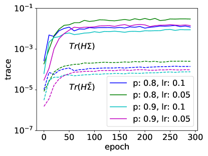
Figure 1: Comparison between $\operatorname{Tr}(\bm{H}_{i}\bm{\Sigma}_{i})$ and $\operatorname{Tr}(\bm{H}_{i}\bar{\bm{\Sigma}}_{i})$ in each training epoch $i$ for different choices of $p$ and learning rate $lr$. The FNN is trained on the MNIST dataset using the first 10000 examples as the training dataset. The solid and the dotted lines represent the value of $\operatorname{Tr}(\bm{H}_{i}\bm{\Sigma}_{i})$ and $\operatorname{Tr}(\bm{H}_{i}\bar{\bm{\Sigma}}_{i})$, respectively.

5.2.3 Inverse variance-flatness relation

The alignment relation studied above also implies the inverse variance-flatness relation, i.e., the noise variance is large along the sharp direction of the loss landscape, and small along the flat direction. In this subsection, we verify this relation by two sets of experiments. Firstly, we present two different approaches to characterize the flatness of loss landscape and the covariance of noise from the random trajectory data $\mathcal{D}_{\rm para}$ and random gradient data $\mathcal{D}_{\rm grad}$, then we numerically demonstrate the inverse variance-flatness relation. Due to space limitations, we defer the experiments on ResNet and Transformer to Appendix B. For convenience, $\mathcal{D}$ refers to either the dataset $\mathcal{D}_{\rm para}$ or the dataset $\mathcal{D}_{\rm para}$ depending on its context, so is the case for their corresponding covariance $\bm{\Sigma}$ and Hessian $\bm{H}$. We then proceed to the definitions of noise variance and interval flatness.

Definition 2 (noise variance).

For dataset $\mathcal{D}$ and its covariance $\bm{\Sigma}$, we denote $\lambda_{i}(\bm{\Sigma})$ as the $i$th eigenvalue of $\bm{\Sigma}$ and its corresponding eigen direction as $\bm{v}_{i}(\bm{\Sigma})$. Then we term $\lambda_{i}(\bm{\Sigma})$ the noise variance of $\mathcal{D}$ at the eigen direction $\bm{v}_{i}(\bm{\Sigma})$.

The interval flatness below characterizes the flatness of the landscape around a local minimum.

Definition 3 (interval flatness ).

For a a local minimum $\bm{\theta}^{*}_{0}$, the loss function profile $R_{\bm{v}}$ along direction $\bm{v}$ reads:

$$R_{\bm{v}}(\delta)\equiv R_{S}(\bm{\theta}^{*}_{0}+\delta\bm{v}),$$

where $\delta$ represents the distance moved in the $\bm{v}$ direction. The interval flatness $F_{\bm{v}}$ is then defined as the width of the region within which $R_{\bm{v}}(\delta)\leq 2R_{\bm{v}}(0)$. We determine $F_{\bm{v}}$ by finding two closest points $\theta_{\bm{v}}^{l}<0$ and $\theta_{\bm{v}}^{r}>0$ on each side of the minimum that satisfy $R_{\bm{v}}(\theta_{\bm{v}}^{l})=R_{\bm{v}}(\theta_{\bm{v}}^{r})=2R_{\bm{v}}(0)$. The interval flatness is defined as:

$$F_{\bm{v}}\equiv\theta_{\bm{v}}^{r}-\theta_{\bm{v}}^{l}.$$ (16)

Remark.

The experiments show that the result is not sensitive to the selection of the pre-factor 2. A larger value of $F_{\bm{v}}$ means a flatter landscape in the direction $\bm{v}$.

We use PCA to study the weight variations when the training accuracy is nearly $100\%$. The networks are trained with full-batch GD for different learning rates and dropout rates under the same random seed. When the loss is small enough, we sample the parameters or gradients of parameters $N$ times ($N=3000$ for this experiment) and study the relationship between $\{\lambda_{i}(\bm{\Sigma})\}_{i=1}^{N}$ and $\{F_{\bm{v}_{i}(\bm{\Sigma})}\}_{i=1}^{N}$ for both weight dataset $\mathcal{D}_{\rm para}$ and gradient dataset $\mathcal{D}_{\rm grad}$.

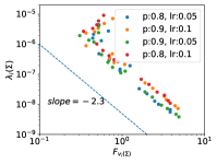
(a) FNN, $\mathcal{D}=\mathcal{D}_{\rm para}$

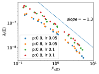
(b) FNN, $\mathcal{D}=\mathcal{D}_{\rm grad}$

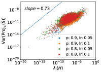
(c) FNN, $\mathcal{D}=\mathcal{D}_{\rm para}$

(d) FNN, $\mathcal{D}=\mathcal{D}_{\rm grad}$

Figure 2: (a, b)The inverse relation between the variance $\{\lambda_{i}(\bm{\Sigma})\}_{i=1}^{N}$ and the interval flatness $\{F_{\bm{v}_{i}(\bm{\Sigma})}\}_{i=1}^{N}$ for different choices of $p$ and learning rate $lr$ with different network structures. The PCA is done for different datasets $\mathcal{D}$ sampled from parameters for the top line and sampled from gradients of parameters for the bottom line. The dashed lines give the approximate slope of the scatter. (c, d)The relation between the variance $\{{\rm Var}({\rm Proj}_{\bm{v}_{i}(\bm{H})}(\mathcal{D}))\}_{i=1}^{N}$ and the eigenvalue $\{\lambda_{i}(\bm{H})\}_{i=1}^{N}$ for different choices of $p$ and learning rate $lr$ with different network structures. The projection is done for different datasets $\mathcal{D}$ sampled from parameters for the top line and sampled from gradients of parameters for the bottom line. The dashed lines give the approximate slope of the scatter. Refer to Appendix B for further experiments such as ResNet and Transformer.

For different learning rates and dropout rates, Fig. 2(a, b) reveal an inverse relationship between the interval flatness of the loss landscape denoted as $\{F_{\bm{v}_{i}(\bm{\Sigma})}\}_{i=1}^{N}$, and the noise variance represented by the PCA spectrum $\{\lambda_{i}(\bm{\Sigma})\}_{i=1}^{N}$. Notably, a power-law relationship can be established between $\{F_{\bm{v}_{i}(\bm{\Sigma})}\}_{i=1}^{N}$ and $\{\lambda_{i}(\bm{\Sigma})\}_{i=1}^{N}$. Specifically, in the low flatness region, the dropout-induced noise exhibits a large variance. As the loss landscape transitions into the high flatness regime, the linear relationship between variance and flatness becomes more evident. Overall, These findings consistently demonstrate the inverse relation between variance and flatness, as exemplified in Fig. 2(a, b). Subsequently, we delve into the definitions of Projected variance and Hessian flatness.

Definition 4 (projected variance).

For a given direction $\bm{v}\in\mathbb{R}^{D}$ and dataset $\mathcal{D}=\{\bm{\theta}_{i}\}_{i=1}^{N}$, where $\bm{\theta}_{i}\in\mathbb{R}^{D}$, the inner product of $\bm{v}$ and $\bm{\theta}_{i}$ is denoted by ${\rm Proj}_{\bm{v}}(\bm{\theta}_{i}):=\left<\bm{\theta}_{i},\bm{v}\right>$, then we can define the projected variance for $\mathcal{D}$ at the direction $\bm{v}$ as follows,

$${\rm Var}({\rm Proj}_{\bm{v}}(\mathcal{D}))=\frac{\sum_{i=1}^{N}({\rm Proj}_{\bm{v}}(\bm{\theta}_{i})-\bm{\mu})^{2}}{N},$$

where $\bm{\mu}$ is the mean value of $\{{\rm Proj}_{\bm{v}}(\bm{\theta}_{i})\}_{i=1}^{N}$.

Definition 5 (Hessian flatness).

For Hessian $\bm{H}$, as we denote $\lambda_{i}(\bm{H})$ by the $i$-th eigenvalue of $\bm{H}$ corresponding to the eigenvector $\bm{v}_{i}(\bm{H})$, we term $\lambda_{i}(\bm{H})$ the Hessian flatness along direction $\bm{v}_{i}(\bm{H})$.

The eigenvalues of the Hessian evaluated at a local minimum often serve as indicators of the flatness of the loss landscape, and larger eigenvalues correspond to sharper directions. In our investigation, we analyze the interplay between the eigenvalues of Hessian $\bm{H}$ at the final stage of the training process and the projected variance of dropout at each of the corresponding eigen directions, i.e., $\lambda_{i}(\bm{H})$ v.s. $\{{\rm Var}({\rm Proj}_{\bm{v}_{i}(\bm{H})}(\mathcal{D}))\}_{i=1}^{N}$. Specifically, we sample the parameters or gradients of parameters $N$ times ($N=1000$ for this experiment), and examine the relationship between $\{\lambda_{i}(\bm{H})\}_{i=1}^{N}$ and $\{{\rm Var}({\rm Proj}_{\bm{v}_{i}(\bm{H})}(\mathcal{D}))\}_{i=1}^{N}$ for both the parameter dataset $\mathcal{D}_{\rm para}$ and the gradient dataset $\mathcal{D}_{\rm grad}$.

Under various dropout rates and learning rates, Fig. 2(c, d) presents establishes a consistent power-law relationship between $\{\lambda_{i}(\bm{H})\}_{i=1}^{N}$ and $\{{\rm Var}({\rm Proj}_{\bm{v}_{i}(\bm{H})}(\mathcal{D}))\}_{i=1}^{N}$, and this relationship remains robust irrespective of the choice between parameter dataset $\mathcal{D}_{\rm para}$ or the gradient dataset $\mathcal{D}_{\rm grad}$. The positive correlation observed between the Hessian flatness and the projection variance provides insights into the structural characteristics of the dropout-induced noise. Specifically, these characteristics have the potential to facilitate the escape from sharp minima and enhance the generalization capabilities of NNs. Additionally, Fig. 2 highlights the distinct linear structure exhibited by gradient sampling in comparison to parameter sampling, which corroborates the discussions outlined in Section 5.2.1. For detailed experimental evidence, including our investigations involving ResNet and Transformer models, one may refer to Appendix B.

6 Conclusion

Our main contribution is twofold. First, we derive the SMEs that provide a weak approximation for the dynamics of the dropout algorithm for two-layer NNs. Second, we demonstrate that dropout exhibits the inverse variance-flatness relation and the Hessian-variance alignment relation through extensive empirical analysis, which is consistent with SGD. These relations are widely recognized to be beneficial for finding flatter minima, thus implying that dropout acts as an implicit regularizer that enhances the generalization abilities.

Given the broad applicability of the methodologies employed in our proof, we aim to extend the formulations of SMEs to an even wider class of stochastic algorithms applied to NNs with different architectures. Such an extension could help us better understand the role of stochastic algorithms in NN training. Moreover, the SME framework could offer a promising approach to the examination of the underlying mechanisms that explain the observed inverse variance-flatness relation and Hessian-variance relation and beyond.

Appendix A Experimental setups

For Fig. 1, Fig. 2, we use the FNN with size $784$-$50$-$50$-$10$ for the MNIST classification task. We train the network using GD with the first $10000$ images as the training set. We add a dropout layer behind the second layer. The dropout rate and learning rate are specified and unchanged in each experiment. We only consider the parameter matrix corresponding to the weight and the bias of the fully-connected layer between two hidden layers. Therefore, for experiments in Fig. 1, $D=2500$.

For Fig. 3(a, c, e, g), we add dropout layers after the convolutional layers, and for each dropout layer, $p=0.8$. We only consider the parameter matrix corresponding to the weight of the first convolutional layer of the first block of the ResNet-20. Models are trained using full-batch GD on the CIFAR100 classification task for $1200$ epochs. The learning rate is initialized at $0.01$. Since the Hessian calculation of ResNet takes much time, we only perform it at a specific dropout rate and learning rate.

For Fig. 3(b, d, f, h), we use transformer Vaswani et al. (2017) with $d_{\mathrm{model}}=50,d_{k}=d_{v}=20,d_{\mathrm{ff}}=256,h=4,N=3$, the meaning of the parameters is consistent with the original paper. We only consider the parameter matrix corresponding to the weight of the fully-connected layer whose output is queried in the Multi-Head Attention layer of the first block of the decoder. We apply dropout to the output of each sub-layer before it is added to the sub-layer input and normalized. In addition, we apply dropout to the sums of the embeddings and the positional encodings in both the encoder and decoder stacks. For each dropout layer, $p=0.9$. For the English-German translation problem, we use the cross-entropy loss with label smoothing trained by full-batch Adam based on the Multi30k dataset. The learning rate strategy is the same as that in Vaswani et al. (2017). The warm-up step is $4000$ epochs, the training step is $10000$ epochs. We only use the first $2048$ examples for training to compromise with the computational burden.

Appendix B Extended experiments on verifying the inverse flatness

In this section, we verify the inverse relation between the covariance matrix and the Hessian matrix of dropout through different data collection methods and projection methods on larger network structures, such as ResNet-20 and transformer, and more complex datasets, such as CIFAR-100 and Multi30k, as shown in Fig. 3.

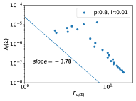
(a) ResNet-20, $D=D_{\rm para}$

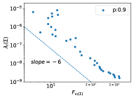
(b) Transformer, $D=D_{\rm para}$

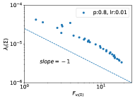
(c) ResNet-20, $D=D_{\rm grad}$

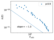
(d) Transformer, $D=D_{\rm grad}$

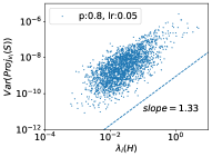
(e) ResNet-20, $D=D_{\rm para}$

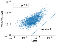
(f) Transformer, $D=D_{\rm para}$

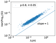
(g) ResNet-20, $D=D_{\rm grad}$

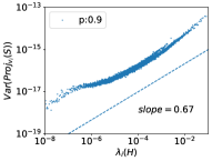
(h) Transformer, $D=D_{\rm grad}$

Figure 3: (a, b, c, d) The inverse relation between the variance $\{\lambda_{i}(\bm{\Sigma})\}_{i=1}^{N}$ and the interval flatness $\{F_{\bm{v}_{i}(\bm{\Sigma})}\}_{i=1}^{N}$ for different choices of $p$ and learning rate $lr$ with different network structures. The PCA is done for different datasets $D$ sampled from parameters for the top line and sampled from gradients of parameters for the bottom line. The dashed lines give the approximate slope of the scatter. (e, f, g, h) The relation between the variance $\{{\rm Var}({\rm Proj}_{\bm{v}_{i}(H)}(D))\}_{i=1}^{N}$ and the eigenvalue $\{\lambda_{i}(H)\}_{i=1}^{N}$ for different choices of $p$ and learning rate $lr$ with different network structures. The projection is done for different datasets $D$ sampled from parameters for the top line and sampled from gradients of parameters for the bottom line. The dashed lines give the approximate slope of the scatter.

Appendix C Preliminaries

C.1 Notations

We adhere wherever possible to the following notation. Dimensional indices are written as subscripts with a bracket to avoid confusion with other sequential indices (e.g. time, iteration number), which do not have brackets. When more than one indices are present, we separate them with a comma, e.g. $\bm{x}_{k,(i)}$ is the $i$-th coordinate of the vector $\bm{x}_{k}$, the $k^{\text{th }}$ member of a sequence.

We set a special vector $(1,1,1,\dots,1)^{\intercal}$ by $\bm{1}:=(1,1,1,\dots,1)^{\intercal}$ whose dimension varies. We set $n$ for the number of input samples, $m$ for the width of the neural network, and $D:=m(d+1)$ hereafter in this paper. We let $[n]=\{1,2,\ldots,n\}$. We set $\mathcal{N}(\bm{\mu},\bm{\Sigma})$ as the normal distribution with mean $\bm{\mu}$ and covariance $\bm{\Sigma}$. We denote $\otimes$ as the Kronecker tensor product, $\left<\cdot,\cdot\right>$ for standard inner product between two vectors, and $\bm{A}:\bm{B}$ for the Frobenius inner product between two matrices $\bm{A}$ and $\bm{B}$. We denote vector $L^{2}$ norm as $\left\lVert\cdot\right\rVert_{2}$, vector or function $L_{\infty}$ norm as $\left\lVert\cdot\right\rVert_{\infty}$, function $L_{1}$ norm as $\left\lVert\cdot\right\rVert_{1}$, matrix infinity norm as $\left\lVert\cdot\right\rVert_{\infty\to\infty}$, matrix spectral (operator) norm as $\left\lVert\cdot\right\rVert_{2\to 2}$, and matrix Frobenius norm as $\left\lVert\cdot\right\rVert_{\mathrm{F}}.$ Finally, we denote the set of continuous functions $f(\cdot):\mathbb{R}^{D}\to\mathbb{R}$ possessing continuous derivatives of order up to and including $r$ by $\mathcal{C}^{r}(\mathbb{R}^{D})$, and for a Polish space $\mathcal{X}$, we denote the space of bounded measurable functions by $\mathcal{B}_{b}(\mathcal{X})$, and the space of bounded continuous functions by $\mathcal{C}_{b}(\mathcal{X})$. In the mathematical discipline of general topology, a Polish space is a separable complete metric space.

C.2 Problem Setup

For the empirical risk minimization problem given by the quadratic loss:

$$\min_{\bm{\theta}}R_{\mathcal{S}}(\bm{\theta})=\frac{1}{2n}\sum_{i=1}^{n}\left({f_{\bm{\theta}}(\bm{x}_{i})-y_{i}}\right)^{2},$$ (17)

where $\mathcal{S}:=\{(\bm{x}_{i},y_{i})\}_{i=1}^{n}$ is the training sample, $f_{\bm{\theta}}(\bm{x})$ is the prediction function, $\bm{\theta}$ are the parameters to be optimized over, and their dependence is modeled by a two-layer neural network (NN) with $m$ hidden neurons

$$f_{\bm{\theta}}(\bm{x}):=\sum_{r=1}^{m}a_{r}\sigma(\bm{w}_{r}^{\intercal}\bm{x}),$$ (18)

where $\bm{x}\in\mathbb{R}^{d}$, $\bm{\theta}=\mathrm{vec}(\bm{\theta}_{a},\bm{\theta}_{\bm{w}})$ with $\bm{\theta}_{a}=\mathrm{vec}(\{a_{r}\}_{r=1}^{m})$, $\bm{\theta}_{\bm{w}}=\mathrm{vec}(\{\bm{w}_{r}\}_{r=1}^{m})$ is the set of parameters, $\sigma(\cdot)$ is the activation function applied coordinate-wisely to its input, and $\sigma$ is $1$-Lipschitz with $\sigma\in\mathcal{C}^{\infty}(\mathbb{R})$. More precisely, $\bm{\theta}=\mathrm{vec}(\{\bm{q}_{r}\}_{r=1}^{m})$ whereas for each $r\in[m]$, $\bm{q}_{r}:=(a_{r},\bm{w}_{r}^{\intercal})^{\intercal}$. We remark that the bias term $b_{r}$ can be incorporated by expanding $\bm{x}$ and $\bm{w}_{r}$ to $(\bm{x}^{\intercal},1)^{\intercal}$ and $\left(\bm{w}_{r}^{\intercal},b_{r}\right)^{\intercal}$.

Given fixed learning rate $\varepsilon>0$, then at the $N$-th iteration, where

$$t_{N}:=N\varepsilon,$$

and a scaling vector $\bm{\eta}_{N}\in\mathbb{R}^{m}$ is sampled with independent random coordinates: For each $k\in[m]$,

$$(\bm{\eta}_{N})_{k}=\begin{cases}\frac{1}{p}&\text{ with probability }p,\\ 0&\text{ with probability }1-p,\end{cases}$$ (19)

and we observe that $\{\bm{\eta}_{N}\}_{N\geq 1}$ is an i.i.d. Bernulli sequence with $\mathbb{E}\bm{\eta}_{1}=\bm{1}$, and naturally, with slight abuse of notations, the $\sigma$-fields $\mathcal{F}_{N}:=\left\{\sigma(\bm{\eta}_{1},\bm{\eta}_{2},\cdots\bm{\eta}_{N})\right\}$ forms a filtration.

We then apply dropout to two-layer NNs by computing

$$\bm{f}_{\bm{\theta}}(\bm{x};\bm{\eta}):=\sum_{r=1}^{m}(\bm{\eta})_{r}a_{r}\sigma(\bm{w}_{r}^{\intercal}\bm{x}),$$ (20)

and we denote the empirical risk associated with dropout by

$$R_{\mathcal{S}}^{\mathrm{drop}}\left(\bm{\theta};\bm{\eta}\right): =\frac{1}{2n}\sum_{i=1}^{n}\left(\bm{f}_{\bm{\theta}}(\bm{x}_{i};\bm{\eta})-y_{i}\right)^{2}$$ (21)

$$=\frac{1}{2n}\sum_{i=1}^{n}\left(\sum_{r=1}^{m}(\bm{\eta})_{r}a_{r}\sigma(\bm{w}_{r}^{\intercal}\bm{x}_{i})-y_{i}\right)^{2}.$$

We observe that the parameters at the $N$-th step are updated via back propagation as follows:

$$\bm{\theta}_{N}=\bm{\theta}_{N-1}-\varepsilon\nabla_{\bm{\theta}}R_{\mathcal{S}}^{\mathrm{drop}}\left(\bm{\theta}_{N-1};\bm{\eta}_{N}\right),$$ (22)

where $\bm{\theta}_{0}:=\bm{\theta}(0)$. Finally, we denote hereafter that for all $i\in[n]$,

$$e_{i}^{N}:=e_{i}(\bm{\theta}_{N-1};\bm{\eta}_{N}):=\bm{f}_{\bm{\theta}_{N-1}}(\bm{x}_{i};\bm{\eta}_{N})-y_{i},$$

hence the empirical risk associated with dropout $R_{\mathcal{S}}^{\mathrm{drop}}\left(\bm{\theta}_{N-1};\bm{\eta}_{N}\right)$ can be written into

$$R_{\mathcal{S}}^{\mathrm{drop}}\left(\bm{\theta}_{N-1};\bm{\eta}_{N}\right)=\frac{1}{2n}\sum_{i=1}^{n}\left(e_{i}^{N}\right)^{2},$$

thus the dropout iteration (22) reads

$$\bm{\theta}_{N}-\bm{\theta}_{N-1} =-\varepsilon\nabla_{\bm{\theta}}R_{\mathcal{S}}^{\mathrm{drop}}\left(\bm{\theta}_{N-1};\bm{\eta}_{N}\right)=-\frac{\varepsilon}{n}\sum_{i=1}^{n}e_{i}^{N}\nabla_{\bm{\theta}}e_{i}^{N},$$

and we may proceed to the introduction of the stochastic modified equation (SME) approximation.

Appendix D Stochastic Modified Equations for Dropout

D.1 Modified Loss

Recall that the parameters at the $N$-th step are updated as follows:

$$\bm{\theta}_{N}=\bm{\theta}_{N-1}-\frac{\varepsilon}{n}\sum_{i=1}^{n}e_{i}^{N}\nabla_{\bm{\theta}}e_{i}^{N},$$ (23)

and since $\{\bm{\eta}_{N}\}_{N\geq 1}$ is an i.i.d.  sequence, then the dropout iteration (23) updates the parameters in a recursion form of

$$\bm{\theta}_{N}=\bm{F}(\bm{\theta}_{N-1},\bm{\eta}_{N}),$$ (24)

where $\bm{F}(\cdot,\cdot):\mathbb{R}^{D}\times\mathbb{R}^{m}\to\mathbb{R}^{D}$ is a smooth ($\mathcal{C}^{\infty}$) function, and $\{\bm{\eta}_{N}\}_{N\geq 1}$ is a disturbance sequence on $\mathbb{R}^{m}$, whose marginal distribution possesses a density supported on an open subset of $\mathbb{R}^{m}$. Then, based on the results in Meyn and Tweedie (2012), the dropout iterations (23) forms a time-homogeneous Markov chain. Thus, we may misuse $\mathbb{E}[\cdot\mid\mathcal{F}_{N}]$, the conditional expectation given $\mathcal{F}_{N}$, with $\mathbb{E}_{\bm{\theta}_{N-1}}[\cdot]$, the conditional expectation given $\bm{\theta}_{N-1}$. Then, for each $k\in[m]$, the conditional expectation of the increment restricted to $\bm{q}_{k}$ reads

$$\mathbb{E}_{\bm{\theta}_{N-1}}\left[\sum_{i=1}^{n}e_{i}^{N}\nabla_{\bm{q}_{k}}e_{i}^{N}\right] =\mathbb{E}_{\bm{\theta}_{N-1}}\left[\sum_{i=1}^{n}e_{i}^{N}(\bm{\eta}_{N})_{k}\nabla_{\bm{q}_{k}}\left(a_{k}\sigma(\bm{w}_{k}^{\intercal}\bm{x}_{i})\right)\right],$$

and since

$$\mathbb{E}_{\bm{\theta}_{N-1}}\left[e_{i}^{N}(\bm{\eta}_{N})_{k}\right] =\mathbb{E}_{\bm{\theta}_{N-1}}\left[\sum_{r=1,r\neq k}^{m}(\bm{\eta}_{N})_{r}a_{r}\sigma(\bm{w}_{r}^{\intercal}\bm{x}_{i})-y_{i}\right]\mathbb{E}_{\bm{\theta}_{N-1}}\left[(\bm{\eta}_{N})_{k}\right]$$

$$~{}~{}+\mathbb{E}_{\bm{\theta}_{N-1}}\left[(\bm{\eta}_{N})_{k}^{2}\right]a_{k}\sigma(\bm{w}_{k}^{\intercal}\bm{x}_{i})$$

$$=\left(\sum_{r=1,r\neq k}^{m}a_{r}\sigma(\bm{w}_{r}^{\intercal}\bm{x}_{i})-y_{i}\right)+\frac{1}{p}a_{k}\sigma(\bm{w}_{k}^{\intercal}\bm{x}_{i})$$

$$=\left(\sum_{r=1}^{m}a_{r}\sigma(\bm{w}_{r}^{\intercal}\bm{x}_{i})-y_{i}\right)+\left(\frac{1}{p}-1\right)a_{k}\sigma(\bm{w}_{k}^{\intercal}\bm{x}_{i}).$$

For simplicity, given fixed $k\in[m]$, for any $i\in[n]$, we denote hereafter that

$$e_{i} :=e_{i}(\bm{\theta}):=\sum_{r=1}^{m}a_{r}\sigma(\bm{w}_{r}^{\intercal}\bm{x}_{i})-y_{i},$$

$$e_{i,\backslash k} :=e_{i,\backslash k}(\bm{\theta}):=\sum_{r=1,r\neq k}^{m}a_{r}\sigma(\bm{w}_{r}^{\intercal}\bm{x}_{i})-y_{i},$$

we remark that compared with $e_{i}^{N}$, $e_{i}$ and $e_{i,\backslash k}$ do not depend on the random variable $\bm{\eta}_{N}$. Then $\mathbb{E}_{\bm{\theta}_{N-1}}\left(e_{i}^{N}(\bm{\eta}_{N})_{k}\right)$ can be written in short by

$$\mathbb{E}_{\bm{\theta}_{N-1}}\left[e_{i}^{N}(\bm{\eta}_{N})_{k}\right] =e_{i,\backslash k}+\frac{1}{p}a_{k}\sigma(\bm{w}_{k}^{\intercal}\bm{x}_{i})$$ (25)

$$=e_{i}+\left(\frac{1}{p}-1\right)a_{k}\sigma(\bm{w}_{k}^{\intercal}\bm{x}_{i}).$$

Hence for each $k\in[m]$, expectation of the increment restricted to $\bm{q}_{k}$ reads

$$\mathbb{E}_{\bm{\theta}_{N-1}}\left[\sum_{i=1}^{n}e_{i}^{N}(\bm{\eta}_{N})_{k}\nabla_{\bm{q}_{k}}\left(a_{k}\sigma(\bm{w}_{k}^{\intercal}\bm{x}_{i})\right)\right]$$

$$= \sum_{i=1}^{n}e_{i}\nabla_{\bm{q}_{k}}\left(a_{k}\sigma(\bm{w}_{k}^{\intercal}\bm{x}_{i})\right)+\sum_{i=1}^{n}\left(\frac{1}{p}-1\right)a_{k}\sigma(\bm{w}_{k}^{\intercal}\bm{x}_{i})\nabla_{\bm{q}_{k}}\left(a_{k}\sigma(\bm{w}_{k}^{\intercal}\bm{x}_{i})\right),$$

then we define the modified loss $L_{\mathcal{S}}(\cdot):\mathbb{R}^{m(d+1)}\to\mathbb{R}$ for dropout:

$$L_{\mathcal{S}}(\bm{\theta}) :=\frac{1}{2n}\sum_{i=1}^{n}e_{i}^{2}+\frac{1-p}{2np}\sum_{i=1}^{n}\sum_{r=1}^{m}a_{r}^{2}\sigma(\bm{w}_{r}^{\intercal}\bm{x}_{i})^{2},$$ (26)

since as $\bm{\theta}_{N-1}$ is given, then by taking the conditional expectation, increment of the dropout iteration (23) reads

$$\bm{\theta}_{N}-\bm{\theta}_{N-1} =-\varepsilon\mathbb{E}_{\bm{\theta}_{N-1}}\left[\nabla_{\bm{\theta}}R_{\mathcal{S}}^{\mathrm{drop}}\left(\bm{\theta}_{N-1};\bm{\eta}_{N}\right)\right]=-\varepsilon\nabla_{\bm{\theta}}L_{\mathcal{S}}(\bm{\theta})\big{|}_{\bm{\theta}=\bm{\theta}_{N-1}},$$

which implies that in the sense of expectations, $\{\bm{\theta}_{N}\}_{N\geq 0}$ follows close to the gradient descent trajectory of $L_{\mathcal{S}}(\bm{\theta})$ with fixed learning rate $\varepsilon$.

D.2 Stochastic Modified Equations

We then follow the strategy of Li et al. (2017) to derive the stochastic modified equations (SME) for dropout. Firstly, from the results in Section D.1, we observe that given $\bm{\theta}_{N-1}$,

$$\bm{\theta}_{N}-\bm{\theta}_{N-1}=-\varepsilon\nabla_{\bm{\theta}}L_{\mathcal{S}}(\bm{\theta})\big{|}_{\bm{\theta}=\bm{\theta}_{N-1}}+\sqrt{\varepsilon}\bm{V}(\bm{\theta}_{N-1}),$$ (27)

where $L_{\mathcal{S}}(\cdot):\mathbb{R}^{m(d+1)}\to\mathbb{R}$ is the modified loss defined in (26), and $\bm{V}(\cdot):\mathbb{R}^{m(d+1)}\to\mathbb{R}^{m(d+1)}$ is a $m(d+1)$-dimensional random vector, and when given $\bm{\theta}_{N-1}$, $\bm{V}(\bm{\theta}_{N-1})$ has mean $\bm{0}$ and covariance $\varepsilon\bm{\Sigma}(\bm{\theta}_{N-1})$, where $\bm{\Sigma}(\cdot):\mathbb{R}^{m(d+1)}\to\mathbb{R}^{m(d+1)\times{m(d+1)}}$ is the covariance of $\nabla_{\bm{\theta}}R_{\mathcal{S}}^{\mathrm{drop}}\left(\bm{\theta}_{N-1};\bm{\eta}_{N}\right)$. Recall that $\bm{\theta}=\mathrm{vec}(\{\bm{q}_{r}\}_{r=1}^{m})=\mathrm{vec}\left(\{(a_{r},\bm{w}_{r})\}_{r=1}^{m}\right)$, and for any $k,r\in[m]$, we denote that

$$\bm{\Sigma}_{kr}(\bm{\theta}_{N-1}):=\mathrm{Cov}\left(\nabla_{\bm{q}_{k}}R_{\mathcal{S}}^{\mathrm{drop}}\left(\bm{\theta}_{N-1};\bm{\eta}_{N}\right),\nabla_{\bm{q}_{r}}R_{\mathcal{S}}^{\mathrm{drop}}\left(\bm{\theta}_{N-1};\bm{\eta}_{N}\right)\right),$$

then

$$\bm{\Sigma}=\left[\begin{array}[]{cccc}\bm{\Sigma}_{11}&\bm{\Sigma}_{12}&\cdots&\bm{\Sigma}_{1m}\\ \bm{\Sigma}_{21}&\bm{\Sigma}_{22}&\cdots&\bm{\Sigma}_{2m}\\ \vdots&\vdots&\vdots&\vdots\\ \bm{\Sigma}_{m1}&\bm{\Sigma}_{m2}&\cdots&\bm{\Sigma}_{mm}\end{array}\right].$$

For each $k\in[m]$, we obtain that

$$\bm{\Sigma}_{kk}(\bm{\theta}_{N-1})=\mathrm{Cov}\left(\nabla_{\bm{q}_{k}}R_{\mathcal{S}}^{\mathrm{drop}}\left(\bm{\theta}_{N-1};\bm{\eta}_{N}\right),\nabla_{\bm{q}_{k}}R_{\mathcal{S}}^{\mathrm{drop}}\left(\bm{\theta}_{N-1};\bm{\eta}_{N}\right)\right)$$

$$= \left(\frac{1}{p}-1\right)\left(\frac{1}{n}\sum_{i=1}^{n}\left(e_{i,\backslash k}+\frac{1}{p}a_{k}\sigma(\bm{w}_{k}^{\intercal}\bm{x}_{i})\right)\nabla_{\bm{q}_{k}}\left(a_{k}\sigma(\bm{w}_{k}^{\intercal}\bm{x}_{i})\right)\right)$$

$$~{}~{}~{}~{}~{}~{}~{}~{}~{}~{}~{}~{}~{}~{}~{}~{}~{}~{}~{}~{}~{}~{}~{}~{}~{}~{}~{}~{}~{}~{}{\otimes}\left(\frac{1}{n}\sum_{i=1}^{n}\left(e_{i,\backslash k}+\frac{1}{p}a_{k}\sigma(\bm{w}_{k}^{\intercal}\bm{x}_{i})\right)\nabla_{\bm{q}_{k}}\left(a_{k}\sigma(\bm{w}_{k}^{\intercal}\bm{x}_{i})\right)\right)$$

$$~{}+\left(\frac{1}{p^{2}}-\frac{1}{p}\right)\sum_{l=1,l\neq k}^{m}\left(\frac{1}{n}\sum_{i=1}^{n}a_{l}\sigma(\bm{w}_{l}^{\intercal}\bm{x}_{i})\nabla_{\bm{q}_{k}}\left(a_{k}\sigma(\bm{w}_{k}^{\intercal}\bm{x}_{i})\right)\right)$$

$$~{}~{}~{}~{}~{}~{}~{}~{}~{}~{}~{}~{}~{}~{}~{}~{}~{}~{}~{}~{}~{}~{}~{}~{}~{}~{}~{}~{}~{}~{}{\otimes}\left(\frac{1}{n}\sum_{i=1}^{n}a_{l}\sigma(\bm{w}_{l}^{\intercal}\bm{x}_{i})\nabla_{\bm{q}_{k}}\left(a_{k}\sigma(\bm{w}_{k}^{\intercal}\bm{x}_{i})\right)\right),$$

and for each $k,r\in[m]$ with $k\neq r$,

$$\bm{\Sigma}_{kr}(\bm{\theta}_{N-1})=\mathrm{Cov}\left(\nabla_{\bm{q}_{k}}R_{\mathcal{S}}^{\mathrm{drop}}\left(\bm{\theta}_{N-1};\bm{\eta}_{N}\right),\nabla_{\bm{q}_{r}}R_{\mathcal{S}}^{\mathrm{drop}}\left(\bm{\theta}_{N-1};\bm{\eta}_{N}\right)\right)$$

$$= \left(\frac{1}{p}-1\right)\left(\frac{1}{n}\sum_{i=1}^{n}\left(e_{i,\backslash k,\backslash r}+\frac{1}{p}a_{k}\sigma(\bm{w}_{k}^{\intercal}\bm{x}_{i})+\frac{1}{p}a_{r}\sigma(\bm{w}_{r}^{\intercal}\bm{x}_{i})\right)\nabla_{\bm{q}_{k}}\left(a_{k}\sigma(\bm{w}_{k}^{\intercal}\bm{x}_{i})\right)\right)$$

$$~{}~{}~{}~{}~{}~{}~{}~{}~{}~{}~{}~{}~{}~{}~{}~{}{\otimes}\left(\frac{1}{n}\sum_{i=1}^{n}a_{k}\sigma(\bm{w}_{k}^{\intercal}\bm{x}_{i})\nabla_{\bm{q}_{r}}\left(a_{r}\sigma(\bm{w}_{r}^{\intercal}\bm{x}_{i})\right)\right)$$

$$+\left(\frac{1}{p}-1\right)\left(\frac{1}{n}\sum_{i=1}^{n}a_{r}\sigma(\bm{w}_{r}^{\intercal}\bm{x}_{i})\nabla_{\bm{q}_{k}}\left(a_{k}\sigma(\bm{w}_{k}^{\intercal}\bm{x}_{i})\right)\right)$$

$$~{}~{}~{}~{}~{}~{}~{}~{}~{}~{}~{}~{}~{}~{}~{}~{}{\otimes}\left(\frac{1}{n}\sum_{i=1}^{n}\left(e_{i,\backslash k,\backslash r}+a_{k}\sigma(\bm{w}_{k}^{\intercal}\bm{x}_{i})+\frac{1}{p}a_{r}\sigma(\bm{w}_{r}^{\intercal}\bm{x}_{i})\right)\nabla_{\bm{q}_{r}}\left(a_{r}\sigma(\bm{w}_{r}^{\intercal}\bm{x}_{i})\right)\right),$$

where we denote hereafter that

$$e_{i,\backslash k,\backslash r}:=e_{i,\backslash k,\backslash r}(\bm{\theta}):=\sum_{l=1,l\neq k,l\neq r}^{m}a_{l}\sigma(\bm{w}_{l}^{\intercal}\bm{x}_{i})-y_{i},$$

and compared with $e_{i}^{N}$, $e_{i,\backslash k,\backslash r}$ still does not depend on the random variable $\bm{\eta}_{N}$. We remark that the expression above is consistent in that for the extreme case where $p=1$, dropout ‘degenerates’ to gradient descent (GD), hence the covariance matrix degenerates to a zero matrix, i.e., $\bm{\Sigma}=\bm{0}_{D\times D}$. We remark that details for the derivation of $\bm{\Sigma}$ is deferred to Section G.

Now, as we consider the stochastic differential equation (SDE),

$$\mathrm{d}\bm{\Theta}_{t}=\bm{b}\left(\bm{\Theta}_{t}\right)\mathrm{d}t+\bm{\sigma}\left(\bm{\Theta}_{t}\right)\mathrm{d}\bm{W}_{t},\quad\bm{\Theta}_{0}=\bm{\Theta}(0),$$ (28)

where $\bm{W}_{t}$ is a standard $m(d+1)$-dimensional standard Wiener process, whose Euler–Maruyama discretization with step size $\varepsilon>0$ at the $N$-th step reads

$$\bm{\Theta}_{\varepsilon N}=\bm{\Theta}_{\varepsilon(N-1)}+\varepsilon\bm{b}\left(\bm{\Theta}_{\varepsilon(N-1)}\right)+\sqrt{\varepsilon}\bm{\sigma}\left(\bm{\Theta}_{\varepsilon(N-1)}\right)\bm{Z}_{N},$$

where $\bm{Z}_{N}\sim\mathcal{N}(\bm{0},\bm{I}_{m(d+1)})$ and $\bm{\Theta}_{0}=\bm{\Theta}(0)$. Thus, if we set

$$\bm{b}\left(\bm{\Theta}\right) :=-\nabla_{\bm{\Theta}}L_{\mathcal{S}}(\bm{\Theta}),$$ (29)

$$\bm{\sigma}\left(\bm{\Theta}\right) :=\sqrt{\varepsilon}\left(\bm{\Sigma}\left(\bm{\Theta}\right)\right)^{\frac{1}{2}},$$

$$\bm{\Theta}_{0} :=\bm{\theta}_{0},$$

then we would expect (28) to be a ‘good’ approximation of (27) with the time identification $t=\varepsilon N$. Based on the earlier work of Li et al. (2017), since the path of dropout and the counterpart of SDE are driven by noises sampled in different spaces. Firstly, notice that the stochastic process $\left\{\bm{\theta}_{N}\right\}_{N\geq 0}$ induces a probability measure on the product space $\mathbb{R}^{D}\times\mathbb{R}^{D}\times\cdots\times\mathbb{R}^{D}\times\cdots$, whereas $\left\{\bm{\Theta}_{t}\right\}_{t\geq 0}$ induces a probability measure on $\mathcal{C}\left([0,\infty),\mathbb{R}^{D}\right)$. To compare them, one can form a piece-wise linear interpolation of the former. Alternatively, as we do in this work, we sample a discrete number of points from the latter. Secondly, the process $\left\{\bm{\theta}_{N}\right\}_{N\geq 0}$ is adapted to the filtration generated by $\mathcal{F}_{N}$ whereas the process $\left\{\bm{\Theta}_{t}\right\}_{t\geq 0}$ is adapted to an independent Wiener filtration $\mathcal{F}_{t}$. Hence, it is not appropriate to compare individual sample paths. Rather, we define below a sense of weak approximations (Kloeden and Platen, 2011, Section 9.7) by comparing the distributions of the two processes.

To compare different discrete time approximations, we need to take the rate of weak convergence into consideration, and we also need to choose an appropriate class of functions as the space of test functions. We introduce the following set of smooth functions:

$$\mathcal{C}_{b}^{M}\left(\mathbb{R}^{m(d+1)}\right)=\left\{f\in\mathcal{C}^{M}\left(\mathbb{R}^{m(d+1)}\right)\Bigg{|}\left\lVert f\right\rVert_{\mathcal{C}^{M}}:=\sum_{|\beta|\leq M}\left\lVert\mathrm{D}^{\beta}f\right\rVert_{\infty}<\infty\right\},$$

where $\mathrm{D}$ is the usual differential operator. We remark that $\mathcal{C}_{b}^{M}(\mathbb{R}^{D})$ is a subset of $\mathcal{G}(\mathbb{R}^{D})$, the class of functions with polynomial growth, which is chosen to be the space of test functions in previous works (Li et al., 2017; Kloeden and Platen, 2011; Malladi et al., 2022).

Before we proceed to the definition of weak approximation, to ensure the rigor and validity of our analysis, we shall assert an assumption regarding the existence and uniqueness of solutions to the SDE (28).

Assumption 2.

There exists $T^{\ast}>0$, such that for any time $t\in\left[0,T^{\ast}\right]$, there exists a unique $t$-continuous solution $\bm{\Theta}_{t}$ of the initial value problem:

$$\mathrm{d}\bm{\Theta}_{t}=\bm{b}\left(\bm{\Theta}_{t}\right)\mathrm{d}t+\bm{\sigma}\left(\bm{\Theta}_{t}\right)\mathrm{d}\bm{W}_{t},\quad\bm{\Theta}_{0}=\bm{\Theta}(0),$$

with the property that $\bm{\Theta}_{t}$ is adapted to the filtration $\mathcal{F}_{t}$ generated by $\bm{W}_{s}$ for all time $s\leq t$. Furthermore, for any $t\in[0,T^{\ast}]$,

$$\mathbb{E}\int_{0}^{t}\left\lVert\bm{\Theta}_{s}(\cdot)\right\rVert_{2}^{2}\mathrm{d}s<\infty.$$

Moreover, we assume that the second, fourth and sixth moments of the solution to SDE (28) are uniformly bounded with respect to time $t$, i.e., for each $l\in[3]$, there exists $C(T^{\ast},\bm{\Theta}_{0})>0$, such that

$$\sup_{{0}\leq s\leq T^{\ast}}\mathbb{E}\left\lVert\bm{\Theta}_{s}(\cdot)\right\rVert_{2}^{2l}\leq C(T^{\ast},\bm{\Theta}_{0}).$$ (30)

As for the dropout iterations (23), we assume further that the second, fourth and sixth moments of the dropout iterations (23) are uniformly bounded with respect to the number of iterations $N$, i.e., let $0<\varepsilon<1$, $T>0$ and set $N_{T,\varepsilon}:=\lfloor\frac{T}{\varepsilon}\rfloor$, then for each $l\in[3]$, there exists $T^{\ast}>0$ and $\varepsilon_{0}>0$, such that for any given learning rate $\varepsilon\leq\varepsilon_{0}$ and all $N\in[0:N_{T^{\ast},\varepsilon}]$, there exists $C(T^{\ast},\bm{\theta}_{0},\varepsilon_{0})>0$, such that

$$\sup_{{0}\leq N\leq[N_{T^{\ast},\varepsilon}]}\mathbb{E}\left\lVert\bm{\theta}_{N}\right\rVert_{2}^{2l}\leq C(T^{\ast},\bm{\theta}_{0},\varepsilon_{0}).$$ (31)

We remark that if $\mathcal{G}(\mathbb{R}^{D})$ is chosen to be the test functions in Li et al. (2019), then similar relations to (30) and (31) shall be imposed, except that in our cases, we only require the second, fourth and sixth moments to be uniformly bounded, while in their cases, all $2l$-moments are required for $l\geq 1$.Establishments of the validity of Assumption 2 regarding the existence and uniqueness of the SDE will be exhibited in Section F.

The definition of weak approximation is stated out as follows.

Definition 6.

The SDE (28) is an order $\alpha$ weak approximation to the dropout (23), if for every $g\in\mathcal{C}_{b}^{M}\left(\mathbb{R}^{m(d+1)}\right)$, there exists $C>0$ and $\varepsilon_{0}>0$, such that given any $\varepsilon\leq\varepsilon_{0}$ and $T\leq T^{\ast}$, then for all $N\in[N_{T,\varepsilon}]$,

$$\left\lvert\mathbb{E}g(\bm{\Theta}_{\varepsilon N})-\mathbb{E}g(\bm{\theta}_{N})\right\rvert\leq C(T,g,\varepsilon_{0})\varepsilon^{\alpha}.$$ (32)

Appendix E Semigroup and Proof Details for the Main Theorem

In this section, we use a semigroup approach (Feng et al., 2018) to study the time-homogeneous Markov chains (processes) formed by dropout.

E.1 Discrete and Continuous Semigroup

Definition 7.

A Markov operator over a Polish space $\mathcal{X}$ is a bounded linear operator $\mathcal{P}:\mathcal{B}_{b}(\mathcal{X})\to\mathcal{B}_{b}(\mathcal{X})$ satisfying

• $\mathcal{P}\mathbf{1}=\mathbf{1}$;

• $\mathcal{P}\varphi$ is positive whenever $\varphi$ is positive;

• If a sequence $\left\{\varphi_{n}\right\}\subset\mathcal{B}_{b}(\mathcal{X})$ converges pointwise to an element $\varphi\in\mathcal{B}_{b}(\mathcal{X})$, then $\mathcal{P}\varphi_{n}$ converges pointwise to $\mathcal{P}\varphi$;

To demonstrate further inequalities that Markov operators satisfy, we offer the following proposition

Proposition 1.

A Markov operator $\mathcal{P}:\mathcal{B}_{b}(\mathcal{X})\to\mathcal{B}_{b}(\mathcal{X})$ over a Polish space $\mathcal{X}$ satisfies

• $(\mathcal{P}f(\bm{x}))^{+}\leq\mathcal{P}f^{+}(\bm{x})$;

• $(\mathcal{P}f(\bm{x}))^{-}\leq\mathcal{P}f^{-}(\bm{x})$;

• $|\mathcal{P}f(\bm{x})|\leq\mathcal{P}|f(\bm{x})|$.

Moreover, if the Polish space $\mathcal{X}$ is equipped with a measure $\mu$, a function $f:\mathcal{X}\rightarrow\mathbb{R}$ is said to be an element of $\mathcal{L}^{1}(\mathcal{X})$ if

$$\int_{\mathcal{X}}|f|\mathrm{d}\mu<\infty.$$

Then for every $f\in\mathcal{L}^{1}(\mathcal{X})$, the following holds

• $\left\lVert\mathcal{P}f\right\rVert_{1}\leq\left\lVert f\right\rVert_{1}$.

In mathematics, the positive part of a real function is defined by the formula

$$f^{+}(\bm{x})=\max(f(\bm{x}),0)=\begin{cases}f(\bm{x})&\text{ if }f(\bm{x})>0,\\ 0&\text{ otherwise. }\end{cases}$$

Similarly, the negative part of $f$ is defined as

$$f^{-}(\bm{x})=\max(-f(\bm{x}),0)=-\min(f(\bm{x}),0)=\begin{cases}-f(\bm{x})&\text{ if }f(\bm{x})<0,\\ 0&\text{ otherwise. }\end{cases}$$

We proceed to the proof for Proposition 1

Proof.

From the definition of $f^{+}$and $f^{-}$, it follows that

$$(\mathcal{P}f)^{+}=\left(\mathcal{P}f^{+}-\mathcal{P}f^{-}\right)^{+} =\max\left(0,\mathcal{P}f^{+}-\mathcal{P}f^{-}\right)$$

$$\leq\max\left(0,\mathcal{P}f^{+}\right)=\mathcal{P}f^{+}.$$

Similarly, we obtain that

$$(\mathcal{P}f)^{-}=\left(\mathcal{P}f^{+}-\mathcal{P}f^{-}\right)^{-} =\max\left(0,\mathcal{P}f^{-}-\mathcal{P}f^{+}\right)$$

$$\leq\max\left(0,\mathcal{P}f^{-}\right)=\mathcal{P}f^{-}.$$

Hence for the last inequality

$$|\mathcal{P}f| =(\mathcal{P}f)^{+}+(\mathcal{P}f)^{-}$$

$$\leq\mathcal{P}f^{+}+\mathcal{P}f^{-}$$

$$=\mathcal{P}\left(f^{+}+f^{-}\right)=\mathcal{P}|f|.$$

Finally, by integrating the above relation over $\mathcal{X}$, we obtain that

$$\left\lVert\mathcal{P}f\right\rVert_{1} =\int_{\mathcal{X}}\left\lvert\mathcal{P}f\right\rvert\mathrm{d}\mu$$ (33)

$$\leq\int_{\mathcal{X}}\mathcal{P}\left\lvert f\right\rvert\mathrm{d}\mu=\int_{\mathcal{X}}\left\lvert f\right\rvert\mathrm{d}\mu=\left\lVert f\right\rVert_{1}.$$

∎

Inequality (33) is extremely important, and any operator $\mathcal{P}$ that satisfies it is called a contraction. This relation is known as the contractive property of $\mathcal{P}$. To illustrate its power, note that for any $f\in\mathcal{L}^{1}(\mathcal{X})$, we have

$$\left\lVert\mathcal{P}^{n}f\right\rVert_{1}=\left\lVert\mathcal{P}\circ\mathcal{P}^{n-1}f\right\rVert_{1}\leq\left\lVert\mathcal{P}^{n-1}f\right\rVert_{1}.$$

As we consider Markov processes with continuous time, it is natural to consider a family of Markov operators indexed by time. We call such a family a Markov semigroup (Hairer, 2008), provided that it satisfies the relation

$$\mathcal{P}_{t+s}=\mathcal{P}_{t}\circ\mathcal{P}_{s},\quad\text{for~{}any~{}time}~{}s,t>0.$$ (34)

And if given $A\in\mathcal{B}(\mathcal{X})$, where $\mathcal{B}(\mathcal{X})$ is the Borel $\sigma$-algebra on $\mathcal{X}$, and given any two times $s<t$, if the following holds almost surely

$$\mathbb{P}\left(\bm{X}_{t}\in A\mid\bm{X}_{s}\right)=\left(\mathcal{P}_{t-s}\mathbf{1}_{A}\right)\left(\bm{X}_{s}\right),$$

then we call $\bm{X}_{t}$ a time-homogeneous Markov process with semigroup $\left\{\mathcal{P}_{t}\right\}_{t\geq 0}$.

In our case for dropout, we set the Polish space $\mathcal{X}=\mathbb{R}^{D}$, and since $\mathcal{C}_{b}^{M}(\mathbb{R}^{D})\subset\mathcal{B}_{b}(\mathbb{R}^{D})$, then WLOG we fix $g\in\mathcal{C}_{b}^{M}(\mathbb{R}^{D})$ and define

$$\mathcal{P}_{\varepsilon}g(\tilde{\bm{\theta}}):=\mathbb{E}\left[g\left(\tilde{\bm{\theta}}-\varepsilon\nabla_{\bm{\theta}}R_{\mathcal{S}}^{\mathrm{drop}}\left(\bm{\theta};\bm{\eta}\right)\mid_{\bm{\theta}=\tilde{\bm{\theta}}}\right)\right].$$ (35)

We conclude that the dropout iterations (23) forms a time-homogeneous Markov chain with discrete Markov semigroup $\left\{\mathcal{P}_{\varepsilon}^{n}\right\}_{n\geq 0}$.

As for the SDE (28), based on Assumption 2 and combined with the results in (Hairer, 2008, Example 2.11), the Markov semigroup $\left\{\mathcal{P}_{t}\right\}_{t\geq 0}$ associated to the solutions of the SDE reads: For any $g\in\mathcal{B}_{b}(\mathbb{R}^{D})$,

$$\partial_{t}\mathcal{P}_{t}g=\mathcal{L}\mathcal{P}_{t}g,$$

where $\mathcal{L}$ is termed the generator of the diffusion process (28), which reads

$$\mathcal{L}g:=\left<\bm{b},\nabla_{\bm{\Theta}}g\right>+\frac{1}{2}\bm{\sigma}\bm{\sigma}^{\intercal}:\nabla_{\bm{\Theta}}^{2}g.$$ (36)

Moreover, for a fixed test function $g\in\mathcal{C}_{b}^{M}(\mathbb{R}^{D})$, then for any two times $s,t\geq 0$,

$$\mathcal{P}_{t}g(\bm{\Theta}_{s}):=\exp(t\mathcal{L})g(\bm{\Theta}_{s}):=\mathbb{E}_{\bm{\Theta}_{s}}\left[g(\bm{\Theta}_{t+s})\right],$$ (37)

and $\{\mathcal{P}_{t}\}_{t\geq 0}$ forms a continuous Markov semigroup for the SDE (28).

E.2 Semigroup Expansion with Accuracy of Order One

Our results are essentially based on Itô-Taylor expansions (Kloeden and Platen, 2011) or Taylor’s theorem with the Lagrange form of the remainder (Li et al., 2019, Lemma 27).

Theorem 1 (Order-$1$ accuracy).

Fix time $T\leq T^{\ast}$, if we choose

$$\bm{b}\left(\bm{\Theta}\right) :=-\nabla_{\bm{\Theta}}L_{\mathcal{S}}(\bm{\Theta}),$$

$$\bm{\sigma}\left(\bm{\Theta}\right) :=\sqrt{\varepsilon}\left(\bm{\Sigma}\left(\bm{\Theta}\right)\right)^{\frac{1}{2}},$$

then for all $t\in[0,T]$, the stochastic processes $\bm{\Theta}_{t}$ satisfying

$$\mathrm{d}\bm{\Theta}_{t}=\bm{b}\left(\bm{\Theta}_{t}\right)\mathrm{d}t+\bm{\sigma}\left(\bm{\Theta}_{t}\right)\mathrm{d}\bm{W}_{t},\quad\bm{\Theta}_{0}=\bm{\Theta}(0),$$ (38)

is an order-$1$ approximation of dropout (23), i.e., given any test function $g\in\mathcal{C}_{b}^{4}(\mathbb{R}^{D})$, there exists $\varepsilon_{0}>0$ and $C(T,\left\lVert g\right\rVert_{C^{4}},\varepsilon_{0})>0$, such that for any $\varepsilon\leq\varepsilon_{0}$ and $T\leq T^{\ast}$, and for all $N\in[N_{T,\varepsilon}]$, the following holds:

$$\left\lvert\mathbb{E}g(\bm{\theta}_{N})-\mathbb{E}g(\bm{\Theta}_{\varepsilon N})\right\rvert\leq C(T,\left\lVert g\right\rVert_{C^{4}},\bm{\theta}_{0},\varepsilon_{0})\eta,$$ (39)

where $\bm{\theta}_{0}=\bm{\Theta}_{0}$.

Proof.

By application of Taylor’s theorem with the Lagrange form of the remainder, we have that for some $\alpha\geq 1,$

$$g(\bm{\vartheta})-g(\tilde{\bm{\vartheta}}) =\sum_{s=1}^{\alpha}\frac{1}{s!}\sum_{i_{1},\ldots,i_{j}=1}^{D}\prod_{j=1}^{s}\left[\bm{\vartheta}_{\left(i_{j}\right)}-\tilde{\bm{\vartheta}}_{\left(i_{j}\right)}\right]\frac{\partial^{s}g}{\partial\bm{\vartheta}_{\left(i_{1}\right)}\ldots\partial\bm{\vartheta}_{\left(i_{j}\right)}}(\tilde{\bm{\vartheta}})$$

$$~{}~{}+\frac{1}{(\alpha+1)!}\sum_{i_{1},\ldots,i_{j}=1}^{D}\prod_{j=1}^{\alpha+1}\left[\bm{\vartheta}_{\left(i_{j}\right)}-\tilde{\bm{\vartheta}}_{\left(i_{j}\right)}\right]\frac{\partial^{\alpha+1}g}{\partial\bm{\vartheta}_{\left(i_{1}\right)}\ldots\partial\bm{\vartheta}_{\left(i_{j}\right)}}(\gamma\bm{\vartheta}+(1-\gamma)\tilde{\bm{\vartheta}}),$$

for some $\gamma\in(0,1)$. We adopt the Einstein’s summation convention, where repeated (spatial) indices are summed, i.e.,

$$\bm{x}_{(i)}\bm{x}_{(i)}:=\sum_{i=1}^{D}\bm{x}_{(i)}\bm{x}_{(i)}.$$

As we choose $\bm{\vartheta}:=\bm{\theta}_{1}$, $\tilde{\bm{\vartheta}}:=\bm{\theta}_{0}$ and $\alpha=1$, then we obtain that

$$g(\bm{\theta}_{1})-g(\bm{\theta}_{0}) =\left<\nabla_{\bm{\theta}}g(\bm{\theta}_{0}),\bm{\theta}_{1}-\bm{\theta}_{0}\right>$$

$$~{}~{}+\frac{1}{2}\nabla_{\bm{\theta}}^{2}g(\gamma\bm{\theta}_{1}+(1-\gamma)\bm{\theta}_{0}):(\bm{\theta}_{1}-\bm{\theta}_{0})\otimes(\bm{\theta}_{1}-\bm{\theta}_{0})$$

$$=\left<\nabla_{\bm{\theta}}g(\bm{\theta}_{0}),\bm{\theta}_{1}-\bm{\theta}_{0}\right>+\frac{1}{2}\nabla_{\bm{\theta}}^{2}g(\tilde{\bm{\theta}}_{0}):(\bm{\theta}_{1}-\bm{\theta}_{0})\otimes(\bm{\theta}_{1}-\bm{\theta}_{0}),$$

where $\tilde{\bm{\theta}}_{0}:=\gamma\bm{\theta}_{1}+(1-\gamma)\bm{\theta}_{0}$, and we observe that since

$$\bm{\theta}_{1}-\bm{\theta}_{0}=-\varepsilon\nabla_{\bm{\theta}}L_{\mathcal{S}}(\bm{\theta})\big{|}_{\bm{\theta}=\bm{\theta}_{0}}+\sqrt{\varepsilon}\bm{V}(\bm{\theta}_{0}),$$

then

$$\mathbb{E}g(\bm{\theta}_{1})-\mathbb{E}g(\bm{\theta}_{0}) =\left<\nabla_{\bm{\theta}}g(\bm{\theta}_{0}),\mathbb{E}\bm{\theta}_{1}-\mathbb{E}\bm{\theta}_{0}\right>+\frac{1}{2}\mathbb{E}\left[\nabla_{\bm{\theta}}^{2}g(\tilde{\bm{\theta}}_{0}):(\bm{\theta}_{1}-\bm{\theta}_{0})\otimes(\bm{\theta}_{1}-\bm{\theta}_{0})\right]$$

$$=-\varepsilon\left<\nabla_{\bm{\theta}}g(\bm{\theta}_{0}),\nabla_{\bm{\theta}}L_{\mathcal{S}}(\bm{\theta})\big{|}_{\bm{\theta}=\bm{\theta}_{0}}\right>+E_{\varepsilon}^{1}({\bm{\theta}}_{0}),$$

where the remainder term $E_{\varepsilon}^{1}(\cdot):\mathbb{R}^{D}\to\mathbb{R}$, whose expression reads

$$E_{\varepsilon}^{1}({\bm{\theta}}_{0}):=\frac{1}{2}\mathbb{E}\left[\nabla_{\bm{\theta}}^{2}g(\tilde{\bm{\theta}}_{0}):(\bm{\theta}_{1}-\bm{\theta}_{0})\otimes(\bm{\theta}_{1}-\bm{\theta}_{0})\right],$$ (40)

and we remark that $\tilde{\bm{\theta}}_{0}$ and $\bm{\theta}_{1}$ are implicitly defined by $\bm{\theta}_{0}$. Then, directly from Assumption 2, we obtain that

$$E_{\varepsilon}^{1}({\bm{\theta}}_{0}) =\frac{1}{2}\mathbb{E}\left[\nabla_{\bm{\theta}}^{2}g(\tilde{\bm{\theta}}_{0}):(\bm{\theta}_{1}-\bm{\theta}_{0})\otimes(\bm{\theta}_{1}-\bm{\theta}_{0})\right]$$

$$\leq\frac{1}{2}\left\lVert g\right\rVert_{C^{4}}\mathbb{E}\left\lVert\bm{\theta}_{1}-\bm{\theta}_{0}\right\rVert_{2}^{2}=\varepsilon^{2}\left\lVert g\right\rVert_{C^{4}}\mathbb{E}\left[\left\lVert\nabla_{\bm{\theta}}R_{\mathcal{S}}^{\mathrm{drop}}\left(\bm{\theta}_{0};\bm{\eta}_{1}\right)\right\rVert_{2}^{2}\right]$$

$$\leq\varepsilon^{2}\left\lVert g\right\rVert_{C^{4}}C(T^{\ast},\bm{\theta}_{0},\varepsilon_{0}),$$

since $\nabla_{\bm{\theta}}L_{\mathcal{S}}(\bm{\theta})$ and $\bm{\Sigma}\left(\bm{\theta}\right)$ can be bounded above by the second and fourth moments of the dropout iteration (23).

We observe that

$$\bm{\Theta}_{\varepsilon}-\bm{\Theta}_{0} =\int_{0}^{\varepsilon}\bm{b}(\bm{\Theta}_{s})\mathrm{d}s+\int_{0}^{\varepsilon}\bm{\sigma}(\bm{\Theta}_{s})\mathrm{d}\bm{W}_{s}.$$

As we choose $\bm{\vartheta}:=\bm{\Theta}_{\varepsilon}$, $\tilde{\bm{\vartheta}}:=\bm{\Theta}_{0}$ and $\alpha=1$, then we obtain that

$$g(\bm{\Theta}_{\varepsilon})-g(\bm{\Theta}_{0}) =\left<\nabla_{\bm{\Theta}}g(\bm{\Theta}_{0}),\bm{\Theta}_{\varepsilon}-\bm{\Theta}_{0}\right>$$

$$~{}~{}+\frac{1}{2}\nabla_{\bm{\Theta}}^{2}g(\widetilde{\bm{\Theta}}_{0}):(\bm{\Theta}_{\varepsilon}-\bm{\Theta}_{0})\otimes(\bm{\Theta}_{\varepsilon}-\bm{\Theta}_{0}),$$

where

$$\widetilde{\bm{\Theta}}_{0}:=\gamma\bm{\Theta}_{\varepsilon}+(1-\gamma)\bm{\Theta}_{0},$$

for some $\gamma\in(0,1)$. Then

$$\mathbb{E}g(\bm{\Theta}_{\varepsilon})-\mathbb{E}g(\bm{\Theta}_{0})$$

$$= \left<\nabla_{\bm{\Theta}}g(\bm{\Theta}_{0}),\mathbb{E}\bm{\Theta}_{\varepsilon}-\mathbb{E}\bm{\Theta}_{0}\right>+\frac{1}{2}\mathbb{E}\left[\nabla_{\bm{\Theta}}^{2}g(\widetilde{\bm{\Theta}}_{0}):(\bm{\Theta}_{\varepsilon}-\bm{\Theta}_{0})\otimes(\bm{\Theta}_{\varepsilon}-\bm{\Theta}_{0})\right]$$

$$= \left<\nabla_{\bm{\Theta}}g(\bm{\Theta}_{0}),\int_{0}^{\varepsilon}\mathbb{E}[\bm{b}(\bm{\Theta}_{s})]\mathrm{d}s\right>+\frac{1}{2}\mathbb{E}\left[\nabla_{\bm{\Theta}}^{2}g(\widetilde{\bm{\Theta}}_{0}):(\bm{\Theta}_{\varepsilon}-\bm{\Theta}_{0})\otimes(\bm{\Theta}_{\varepsilon}-\bm{\Theta}_{0})\right],$$

and since

$$\left<\nabla_{\bm{\Theta}}g(\bm{\Theta}_{0}),\mathbb{E}[\bm{b}(\bm{\Theta}_{s})]\right> =\left<\nabla_{\bm{\Theta}}g(\bm{\Theta}_{0}),\mathbb{E}[\bm{b}(\bm{\Theta}_{0})]\right>+\int_{0}^{s}\mathcal{L}\left<\nabla_{\bm{\Theta}}g(\bm{\Theta}_{0}),\bm{b}\right>(\bm{\Theta}_{v})\mathrm{d}v,$$

then we obtain that

$$\mathbb{E}g(\bm{\Theta}_{\varepsilon})-\mathbb{E}g(\bm{\Theta}_{0}) =\varepsilon\left<\nabla_{\bm{\Theta}}g(\bm{\Theta}_{0}),\mathbb{E}[\bm{b}(\bm{\Theta}_{0})]\right>+\int_{0}^{\varepsilon}\int_{0}^{s}\mathcal{L}\left<\nabla_{\bm{\Theta}}g(\bm{\Theta}_{0}),\bm{b}\right>(\bm{\Theta}_{v})\mathrm{d}v\mathrm{d}s$$

$$~{}~{}+\frac{1}{2}\mathbb{E}\left[\nabla_{\bm{\Theta}}^{2}g(\widetilde{\bm{\Theta}}_{0}):(\bm{\Theta}_{\varepsilon}-\bm{\Theta}_{0})\otimes(\bm{\Theta}_{\varepsilon}-\bm{\Theta}_{0})\right]$$

$$=\varepsilon\left<\nabla_{\bm{\Theta}}g(\bm{\Theta}_{0}),\bm{b}(\bm{\Theta}_{0})\right>+\varepsilon^{2}\bar{E}_{\varepsilon}^{1}({\bm{\Theta}}_{0}),$$

where the remainder term $\bar{E}_{\varepsilon}^{1}(\cdot):\mathbb{R}^{D}\to\mathbb{R}$, whose expression reads

$$\bar{E}_{\varepsilon}^{1}({\bm{\Theta}}_{0}) :=\int_{0}^{\varepsilon}\int_{0}^{s}\mathcal{L}\left<\nabla_{\bm{\Theta}}g(\bm{\Theta}_{0}),\bm{b}\right>(\bm{\Theta}_{v})\mathrm{d}v\mathrm{d}s$$ (41)

$$~{}~{}+\frac{1}{2}\mathbb{E}\left[\nabla_{\bm{\Theta}}^{2}g(\widetilde{\bm{\Theta}}_{0}):(\bm{\Theta}_{\varepsilon}-\bm{\Theta}_{0})\otimes(\bm{\Theta}_{\varepsilon}-\bm{\Theta}_{0})\right],$$

and we remark that $\widetilde{\bm{\Theta}}_{0}$ and $\bm{\Theta}_{\varepsilon}$ are implicitly defined by $\bm{\Theta}_{0}$. As we choose

$$\bm{b}\left(\bm{\Theta}\right) =-\nabla_{\bm{\Theta}}L_{\mathcal{S}}(\bm{\Theta}),$$

$$\bm{\sigma}\left(\bm{\Theta}\right) =\sqrt{\varepsilon}\left(\bm{\Sigma}\left(\bm{\Theta}\right)\right)^{\frac{1}{2}},$$

then we carry out the computation for $\mathcal{L}\left<\nabla_{\bm{\Theta}}g(\bm{\Theta}_{0}),\bm{b}\right>(\bm{\Theta}_{v})$,

$$\mathcal{L}\left<\nabla_{\bm{\Theta}}g(\bm{\Theta}_{0}),\bm{b}\right>(\bm{\Theta}_{v}) =\left<\nabla_{\bm{\Theta}}L_{\mathcal{S}}(\bm{\Theta}_{v}),\nabla_{\bm{\Theta}}\left<\nabla_{\bm{\Theta}}g(\bm{\Theta}_{0}),\nabla_{\bm{\Theta}}L_{\mathcal{S}}(\bm{\Theta})\right>\mid_{\bm{\Theta}=\bm{\Theta}_{v}}\right>$$

$$~{}~{}+\frac{\varepsilon}{2}\bm{\Sigma}\left(\bm{\Theta}_{v}\right):\nabla^{2}_{\bm{\Theta}}\left(\left<\nabla_{\bm{\Theta}}g(\bm{\Theta}_{0}),\nabla_{\bm{\Theta}}L_{\mathcal{S}}(\bm{\Theta})\right>\right)\mid_{\bm{\Theta}=\bm{\Theta}_{v}},$$

since $\nabla_{\bm{\Theta}}L_{\mathcal{S}}(\bm{\Theta})$, $\nabla^{2}_{\bm{\Theta}}L_{\mathcal{S}}(\bm{\Theta})$, $\nabla^{3}_{\bm{\Theta}}L_{\mathcal{S}}(\bm{\Theta})$ and $\bm{\Sigma}\left(\bm{\Theta}\right)$ can be bounded above by the second, fourth and sixth moments of the solution to SDE (28), hence we may apply the mean value theorem to (41) and obtain that

$$\left\lvert\bar{E}_{\varepsilon}^{1}({\bm{\Theta}}_{0})\right\rvert =\left\lvert\int_{0}^{\varepsilon}s\mathcal{L}\left<\nabla_{\bm{\Theta}}g(\bm{\Theta}_{0}),\bm{b}\right>({\widetilde{\bm{\Theta}}}_{s})\mathrm{d}s+\frac{1}{2}\mathbb{E}\left[\nabla_{\bm{\Theta}}^{2}g(\widetilde{\bm{\Theta}}_{0}):(\bm{\Theta}_{\varepsilon}-\bm{\Theta}_{0})\otimes(\bm{\Theta}_{\varepsilon}-\bm{\Theta}_{0})\right]\right\rvert$$

$$\leq\int_{0}^{\varepsilon}s\left\lVert g\right\rVert_{C^{4}}C(T^{\ast},\bm{\Theta}_{0})\mathrm{d}s+\frac{1}{2}\left\lVert g\right\rVert_{C^{4}}\mathbb{E}\left\lVert\bm{\Theta}_{\varepsilon}-\bm{\Theta}_{0}\right\rVert_{2}^{2}$$

$$\leq\frac{\varepsilon^{2}}{2}\left\lVert g\right\rVert_{C^{4}}C(T^{\ast},\bm{\Theta}_{0})+\left\lVert g\right\rVert_{C^{4}}\mathbb{E}\left\lVert\int_{0}^{\varepsilon}\bm{b}(\bm{\Theta}_{s})\mathrm{d}s+\int_{0}^{\varepsilon}\bm{\sigma}(\bm{\Theta}_{s})\mathrm{d}\bm{W}_{s}\right\rVert_{2}^{2}$$

$$\leq\frac{\varepsilon^{2}}{2}\left\lVert g\right\rVert_{C^{4}}C(T^{\ast},\bm{\Theta}_{0})+2\left\lVert g\right\rVert_{C^{4}}\mathbb{E}\left\lVert\int_{0}^{\varepsilon}\bm{b}(\bm{\Theta}_{s})\mathrm{d}s\right\rVert_{2}^{2}$$

$$~{}~{}+2\left\lVert g\right\rVert_{C^{4}}\mathbb{E}\left\lVert\int_{0}^{\varepsilon}\bm{\sigma}(\bm{\Theta}_{s})\mathrm{d}\bm{W}_{s}\right\rVert_{2}^{2}$$

$$\leq\frac{\varepsilon^{2}}{2}\left\lVert g\right\rVert_{C^{4}}C(T^{\ast},\bm{\Theta}_{0})+2\left\lVert g\right\rVert_{C^{4}}\varepsilon^{2}\mathbb{E}\left\lVert\nabla_{\bm{\Theta}}L_{\mathcal{S}}(\widetilde{\bm{\Theta}}_{0})\right\rVert_{2}^{2}$$

$$~{}~{}+2\left\lVert g\right\rVert_{C^{4}}\mathbb{E}\int_{0}^{\varepsilon}\left\lVert\bm{\sigma}(\bm{\Theta}_{s})\right\rVert_{\mathrm{F}}^{2}\mathrm{d}s$$

$$\leq\frac{\varepsilon^{2}}{2}\left\lVert g\right\rVert_{C^{4}}C(T^{\ast},\bm{\Theta}_{0})+2\left\lVert g\right\rVert_{C^{4}}\varepsilon^{2}\mathbb{E}\left\lVert\nabla_{\bm{\Theta}}L_{\mathcal{S}}(\widetilde{\bm{\Theta}}_{0})\right\rVert_{2}^{2}$$

$$~{}~{}+2\left\lVert g\right\rVert_{C^{4}}\varepsilon\mathbb{E}\left[\varepsilon\left\lVert\bm{\Sigma}(\widetilde{\bm{\Theta}}_{0})\right\rVert_{\mathrm{F}}\right]\leq\varepsilon^{2}\left\lVert g\right\rVert_{C^{4}}C(T^{\ast},\bm{\Theta}_{0}).$$

To sum up for now,

$$\left\lvert\mathbb{E}g(\bm{\theta}_{1})-\mathbb{E}g(\bm{\Theta}_{\varepsilon})\right\rvert =\Big{|}\mathbb{E}g(\bm{\theta}_{0})-\varepsilon\left<\nabla_{\bm{\theta}}g(\bm{\theta}_{0}),\nabla_{\bm{\theta}}L_{\mathcal{S}}(\bm{\theta})\big{|}_{\bm{\theta}=\bm{\theta}_{0}}\right>+E_{\varepsilon}^{1}({\bm{\theta}}_{0})$$

$$~{}~{}-\mathbb{E}g(\bm{\Theta}_{0})-\varepsilon\left<\nabla_{\bm{\Theta}}g(\bm{\Theta}_{0}),\bm{b}(\bm{\Theta}_{0})\right>+\bar{E}_{\varepsilon}^{1}({\bm{\Theta}}_{0})\Big{|},$$

since $\bm{\theta}_{0}=\bm{\Theta}_{0}$ and $\bm{b}\left(\bm{\Theta}_{0}\right)=-\nabla_{\bm{\Theta}}L_{\mathcal{S}}(\bm{\Theta})\big{|}_{\bm{\theta}=\bm{\theta}_{0}}$, thus

$$\left\lvert\mathcal{P}_{\varepsilon}^{1}g(\bm{\theta}_{0})-\mathcal{P}_{\varepsilon}g(\bm{\Theta}_{0})\right\rvert =\left\lvert\mathbb{E}g(\bm{\theta}_{1})-\mathbb{E}g(\bm{\Theta}_{\varepsilon})\right\rvert$$ (42)

$$\leq\left\lvert E_{\varepsilon}^{1}({\bm{\theta}}_{0})\right\rvert+\left\lvert\bar{E}_{\varepsilon}^{1}({\bm{\Theta}}_{0})\right\rvert$$

$$\leq\varepsilon^{2}\left\lVert g\right\rVert_{C^{4}}C(T^{\ast},\bm{\theta}_{0},\varepsilon_{0})+\varepsilon^{2}\left\lVert g\right\rVert_{C^{4}}C(T^{\ast},\bm{\Theta}_{0})$$

$$=\mathcal{O}(\varepsilon^{2}).$$

For the $N$-th step iteration, since

$$\left\lvert\mathbb{E}g(\bm{\theta}_{N})-\mathbb{E}g(\bm{\Theta}_{\varepsilon N})\right\rvert =\left\lvert\mathcal{P}_{\varepsilon}^{N}g(\bm{\theta}_{0})-\mathcal{P}_{\varepsilon N}g(\bm{\Theta}_{0})\right\rvert,$$

and the RHS of the above equation can be written into a telescoping sum as

$$\mathcal{P}_{\varepsilon}^{N}g(\bm{\theta}_{0})-\mathcal{P}_{\varepsilon N}g(\bm{\Theta}_{0}) =\sum_{l=1}^{N}\left(\mathcal{P}_{\varepsilon}^{N-l+1}\circ\mathcal{P}_{(l-1)\varepsilon}g(\bm{\theta}_{0})-\mathcal{P}_{\varepsilon}^{N-l}\circ\mathcal{P}_{l\varepsilon}g(\bm{\Theta}_{0})\right),$$

hence by application of Proposition 1, we obtain that

$$\left\lvert\mathbb{E}g(\bm{\theta}_{N})-\mathbb{E}g(\bm{\Theta}_{\varepsilon N})\right\rvert \leq\sum_{l=1}^{N}\left\lvert\mathcal{P}_{\varepsilon}^{N-l+1}\circ\mathcal{P}_{(l-1)\varepsilon}g(\bm{\theta}_{0})-\mathcal{P}_{\varepsilon}^{N-l}\circ\mathcal{P}_{l\varepsilon}g(\bm{\Theta}_{0})\right\rvert$$

$$\leq\sum_{l=1}^{N}\left\lvert\mathcal{P}_{\varepsilon}^{N-l}\circ\left(\mathcal{P}_{\varepsilon}^{1}\circ\mathcal{P}_{(l-1)\varepsilon}-\mathcal{P}_{\varepsilon}\circ\mathcal{P}_{(l-1)\varepsilon}\right)g(\bm{\Theta}_{0})\right\rvert,$$

since $\left(\mathcal{P}_{\varepsilon}^{1}\circ\mathcal{P}_{(l-1)\varepsilon}-\mathcal{P}_{\varepsilon}\circ\mathcal{P}_{(l-1)\varepsilon}\right)g(\bm{\Theta}_{0})$ can be regarded as $\mathcal{L}^{1}(\mathbb{R}^{D})$ if we choose measure $\mu$ to be the delta measure concentrated on $\bm{\Theta}_{0}$. i.e.,

$$\mu:=\delta_{\bm{\Theta}_{0}},$$

hence by the conctration property of Markov operators, we obtain further that

$$\left\lvert\mathbb{E}g(\bm{\theta}_{N})-\mathbb{E}g(\bm{\Theta}_{\varepsilon N})\right\rvert \leq\sum_{l=1}^{N}\left\lvert\left(\mathcal{P}_{\varepsilon}^{1}\circ\mathcal{P}_{(l-1)\varepsilon}-\mathcal{P}_{\varepsilon}\circ\mathcal{P}_{(l-1)\varepsilon}\right)g(\bm{\Theta}_{0})\right\rvert$$

$$\leq\sum_{l=1}^{N}\left\lvert\mathcal{P}_{\varepsilon}^{1}g(\bm{\Theta}_{(l-1)\varepsilon})-\mathcal{P}_{\varepsilon}g(\bm{\Theta}_{(l-1)\varepsilon})\right\rvert.$$

By taking expectation conditioned on $\bm{\Theta}_{(l-1)\varepsilon}$, then similar to the relation (42), the following holds

$$\left\lvert\mathcal{P}_{\varepsilon}^{1}g(\bm{\Theta}_{(l-1)\varepsilon})-\mathcal{P}_{\varepsilon}g(\bm{\Theta}_{(l-1)\varepsilon})\right\rvert =\mathbb{E}\left[\left[\left\lvert\mathbb{E}g(\bm{\theta}_{l})-\mathbb{E}g(\bm{\Theta}_{\varepsilon}l)\right\rvert\Big{|}\bm{\Theta}_{(l-1)\varepsilon}\right]\right]$$

$$\leq\mathbb{E}\left\lvert E_{\varepsilon}^{1}(\bm{\Theta}_{(l-1)\varepsilon})\right\rvert+\mathbb{E}\left\lvert\bar{E}_{\varepsilon}^{1}(\bm{\Theta}_{(l-1)\varepsilon})\right\rvert$$

$$\leq\varepsilon^{2}\left\lVert g\right\rVert_{C^{4}}C(T^{\ast},\bm{\theta}_{0},\varepsilon_{0})+\varepsilon^{2}\left\lVert g\right\rVert_{C^{4}}C(T^{\ast},\bm{\Theta}_{0})$$

$$=\mathcal{O}(\varepsilon^{2}).$$

We remark that the last line of the above relation is essentially based on Assumption 2, since $\mathbb{E}\left\lvert E_{\varepsilon}^{1}(\bm{\Theta}_{(l-1)\varepsilon})\right\rvert$ and $\mathbb{E}\left\lvert\bar{E}_{\varepsilon}^{1}(\bm{\Theta}_{(l-1)\varepsilon})\right\rvert$ can be bounded above by the second, fourth and sixth moments of the solution to SDE (28), hence we may apply dominated convergence theorem to obtain the last line of the above relation.

To sum up, as

$$\left\lvert\mathcal{P}_{\varepsilon}^{N}g(\bm{\theta}_{0})-\mathcal{P}_{\varepsilon N}g(\bm{\Theta}_{0})\right\rvert \leq\sum_{l=1}^{N}\left\lvert\mathcal{P}_{\varepsilon}^{N-l+1}\circ\mathcal{P}_{(l-1)\varepsilon}g(\bm{\theta}_{0})-\mathcal{P}_{\varepsilon}^{N-l}\circ\mathcal{P}_{l\varepsilon}g(\bm{\Theta}_{0})\right\rvert=N\mathcal{O}(\varepsilon^{2}),$$

hence for $N=N_{T,\varepsilon}$,

$$\left\lvert\mathcal{P}_{\varepsilon}^{N}g(\bm{\theta}_{0})-\mathcal{P}_{\varepsilon N}g(\bm{\Theta}_{0})\right\rvert=N\mathcal{O}(\varepsilon^{2})=N\varepsilon\mathcal{O}(\varepsilon)\leq T\mathcal{O}(\varepsilon)=\mathcal{O}(\varepsilon).$$

∎

E.3 Semigroup Expansion with Accuracy of Order Two

Theorem 2 (Order-$2$ accuracy).

Fix time $T\leq T^{\ast}$, if we choose

$$\bm{b}(\bm{\Theta}) =-\nabla_{\bm{\Theta}}\left(L_{\mathcal{S}}(\bm{\Theta})+\frac{\varepsilon}{4}\left\lVert\nabla_{\bm{\Theta}}L_{S}(\bm{\Theta})\right\rVert_{2}^{2}\right),$$

$$\bm{\sigma}(\bm{\Theta}) =\sqrt{\varepsilon}\left(\bm{\Sigma}\left(\bm{\Theta}\right)\right)^{\frac{1}{2}},$$

then for all $t\in[0,T]$, the stochastic processes $\bm{\Theta}_{t}$ satisfying

$$\mathrm{d}\bm{\Theta}_{t}=\bm{b}\left(\bm{\Theta}_{t}\right)\mathrm{d}t+\bm{\sigma}\left(\bm{\Theta}_{t}\right)\mathrm{d}\bm{W}_{t},\quad\bm{\Theta}_{0}=\bm{\Theta}(0),$$ (43)

is an order-$2$ approximation of dropout (23), i.e., given any test function $g\in\mathcal{C}_{b}^{6}(\mathbb{R}^{D})$, there exists $\varepsilon_{0}>0$ and $C(T,\left\lVert g\right\rVert_{C^{6}},\varepsilon_{0})>0$, such that for any $\varepsilon\leq\varepsilon_{0}$ and $T\leq T^{\ast}$, and for all $N\in[N_{T,\varepsilon}]$, the following holds:

$$\left\lvert\mathbb{E}g(\bm{\theta}_{N})-\mathbb{E}g(\bm{\Theta}_{\varepsilon N})\right\rvert\leq C(T,\left\lVert g\right\rVert_{C^{6}},\bm{\theta}_{0},\varepsilon_{0})\eta,$$ (44)

where $\bm{\theta}_{0}=\bm{\Theta}_{0}$.

Proof.

By application of Taylor’s theorem with the Lagrange form of the remainder, we have that for some $\alpha\geq 1,$

$$g(\bm{\vartheta})-g(\tilde{\bm{\vartheta}}) =\sum_{s=1}^{\alpha}\frac{1}{s!}\sum_{i_{1},\ldots,i_{j}=1}^{D}\prod_{j=1}^{s}\left[\bm{\vartheta}_{\left(i_{j}\right)}-\tilde{\bm{\vartheta}}_{\left(i_{j}\right)}\right]\frac{\partial^{s}g}{\partial\bm{\vartheta}_{\left(i_{1}\right)}\ldots\partial\bm{\vartheta}_{\left(i_{j}\right)}}(\tilde{\bm{\vartheta}})$$

$$~{}~{}+\frac{1}{(\alpha+1)!}\sum_{i_{1},\ldots,i_{j}=1}^{D}\prod_{j=1}^{\alpha+1}\left[\bm{\vartheta}_{\left(i_{j}\right)}-\tilde{\bm{\vartheta}}_{\left(i_{j}\right)}\right]\frac{\partial^{\alpha+1}g}{\partial\bm{\vartheta}_{\left(i_{1}\right)}\ldots\partial\bm{\vartheta}_{\left(i_{j}\right)}}(\gamma\bm{\vartheta}+(1-\gamma)\tilde{\bm{\vartheta}}),$$

for some $\gamma\in(0,1)$.

As we choose $\bm{\vartheta}:=\bm{\theta}_{1}$, $\tilde{\bm{\vartheta}}:=\bm{\theta}_{0}$ and $\alpha=2$, with slight misuse of the Frobenius inner product notation, we obtain that

$$g(\bm{\theta}_{1})-g(\bm{\theta}_{0}) =\left<\nabla_{\bm{\theta}}g(\bm{\theta}_{0}),\bm{\theta}_{1}-\bm{\theta}_{0}\right>+\frac{1}{2}\nabla_{\bm{\theta}}^{2}g(\bm{\theta}_{0}):(\bm{\theta}_{1}-\bm{\theta}_{0})\otimes(\bm{\theta}_{1}-\bm{\theta}_{0})$$

$$~{}~{}+\frac{1}{6}\nabla_{\bm{\theta}}^{3}g(\gamma\bm{\theta}_{1}+(1-\gamma)\bm{\theta}_{0}):(\bm{\theta}_{1}-\bm{\theta}_{0})\otimes(\bm{\theta}_{1}-\bm{\theta}_{0})\otimes(\bm{\theta}_{1}-\bm{\theta}_{0})$$

$$=\left<\nabla_{\bm{\theta}}g(\bm{\theta}_{0}),\bm{\theta}_{1}-\bm{\theta}_{0}\right>+\frac{1}{2}\nabla_{\bm{\theta}}^{2}g(\bm{\theta}_{0}):(\bm{\theta}_{1}-\bm{\theta}_{0})\otimes(\bm{\theta}_{1}-\bm{\theta}_{0})$$

$$~{}~{}+\frac{1}{6}\nabla_{\bm{\theta}}^{3}g(\tilde{\bm{\theta}}_{0}):(\bm{\theta}_{1}-\bm{\theta}_{0})\otimes(\bm{\theta}_{1}-\bm{\theta}_{0})\otimes(\bm{\theta}_{1}-\bm{\theta}_{0}),$$

where $\tilde{\bm{\theta}}_{0}:=\gamma\bm{\theta}_{1}+(1-\gamma)\bm{\theta}_{0}$, and we observe that since

$$\bm{\theta}_{1}-\bm{\theta}_{0}=-\varepsilon\nabla_{\bm{\theta}}L_{\mathcal{S}}(\bm{\theta})\big{|}_{\bm{\theta}=\bm{\theta}_{0}}+\sqrt{\varepsilon}\bm{V}(\bm{\theta}_{0}),$$

then

$$\mathbb{E}g(\bm{\theta}_{1})-\mathbb{E}g(\bm{\theta}_{0}) =\left<\nabla_{\bm{\theta}}g(\bm{\theta}_{0}),\mathbb{E}\bm{\theta}_{1}-\mathbb{E}\bm{\theta}_{0}\right>+\frac{1}{2}\nabla_{\bm{\theta}}^{2}g({\bm{\theta}}_{0}):\mathbb{E}\left[(\bm{\theta}_{1}-\bm{\theta}_{0})\otimes(\bm{\theta}_{1}-\bm{\theta}_{0})\right]$$

$$~{}~{}+\frac{1}{6}\mathbb{E}\left[\nabla_{\bm{\theta}}^{3}g(\tilde{\bm{\theta}}_{0}):(\bm{\theta}_{1}-\bm{\theta}_{0})\otimes(\bm{\theta}_{1}-\bm{\theta}_{0})\otimes(\bm{\theta}_{1}-\bm{\theta}_{0})\right]$$

$$=-\varepsilon\left<\nabla_{\bm{\theta}}g(\bm{\theta}_{0}),\nabla_{\bm{\theta}}L_{\mathcal{S}}(\bm{\theta})\big{|}_{\bm{\theta}=\bm{\theta}_{0}}\right>$$

$$~{}~{}+\frac{\varepsilon^{2}}{2}\nabla_{\bm{\theta}}^{2}g({\bm{\theta}}_{0}):\left(\nabla_{\bm{\theta}}L_{\mathcal{S}}(\bm{\theta})\big{|}_{\bm{\theta}=\bm{\theta}_{0}}\otimes\nabla_{\bm{\theta}}L_{\mathcal{S}}(\bm{\theta})\big{|}_{\bm{\theta}=\bm{\theta}_{0}}+\bm{\Sigma}(\bm{\theta}_{0})\right)$$

$$~{}~{}+E_{\varepsilon}^{2}({\bm{\theta}}_{0}),$$

where the remainder term $E_{\varepsilon}^{2}(\cdot):\mathbb{R}^{D}\to\mathbb{R}$, whose expression reads

$$E_{\varepsilon}^{2}({\bm{\theta}}_{0}):=\frac{1}{6}\mathbb{E}\left[\nabla_{\bm{\theta}}^{3}g(\tilde{\bm{\theta}}_{0}):(\bm{\theta}_{1}-\bm{\theta}_{0})\otimes(\bm{\theta}_{1}-\bm{\theta}_{0})\otimes(\bm{\theta}_{1}-\bm{\theta}_{0})\right],$$ (45)

and we remark that $\tilde{\bm{\theta}}_{0}$ and $\bm{\theta}_{1}$ are implicitly defined by $\bm{\theta}_{0}$. Then, directly from Assumption 2, we obtain that

$$E_{\varepsilon}^{2}({\bm{\theta}}_{0}) \leq\frac{1}{6}\left\lVert g\right\rVert_{C^{6}}\mathbb{E}\left\lVert\bm{\theta}_{1}-\bm{\theta}_{0}\right\rVert_{2}^{3}=\varepsilon^{3}\left\lVert g\right\rVert_{C^{6}}\mathbb{E}\left[\left\lVert\nabla_{\bm{\theta}}R_{\mathcal{S}}^{\mathrm{drop}}\left(\bm{\theta}_{0};\bm{\eta}_{1}\right)\right\rVert_{2}^{3}\right]$$

$$\leq\varepsilon^{3}\left\lVert g\right\rVert_{C^{6}}C(T^{\ast},\bm{\theta}_{0},\varepsilon_{0}),$$

since $\nabla_{\bm{\theta}}L_{\mathcal{S}}(\bm{\theta})$ and $\bm{\Sigma}\left(\bm{\theta}\right)$ can be bounded above by the second and fourth moments of the dropout iteration (23).

We observe that

$$\bm{\Theta}_{\varepsilon}-\bm{\Theta}_{0} =\int_{0}^{\varepsilon}\bm{b}(\bm{\Theta}_{s})\mathrm{d}s+\int_{0}^{\varepsilon}\bm{\sigma}(\bm{\Theta}_{s})\mathrm{d}\bm{W}_{s}.$$

As we choose $\bm{\vartheta}:=\bm{\Theta}_{\varepsilon}$, $\tilde{\bm{\vartheta}}:=\bm{\Theta}_{0}$ and $\alpha=3$, then we obtain that

$$g(\bm{\Theta}_{\varepsilon})-g(\bm{\Theta}_{0}) =\left<\nabla_{\bm{\Theta}}g(\bm{\Theta}_{0}),\bm{\Theta}_{\varepsilon}-\bm{\Theta}_{0}\right>$$

$$~{}~{}+\frac{1}{2}\nabla_{\bm{\Theta}}^{2}g({\bm{\Theta}}_{0}):(\bm{\Theta}_{\varepsilon}-\bm{\Theta}_{0})\otimes(\bm{\Theta}_{\varepsilon}-\bm{\Theta}_{0})$$

$$~{}~{}+\frac{1}{6}\nabla_{\bm{\Theta}}^{3}g({\bm{\Theta}}_{0}):(\bm{\Theta}_{\varepsilon}-\bm{\Theta}_{0})\otimes(\bm{\Theta}_{\varepsilon}-\bm{\Theta}_{0})\otimes(\bm{\Theta}_{\varepsilon}-\bm{\Theta}_{0})$$

$$~{}~{}+\frac{1}{24}\nabla_{\bm{\Theta}}^{4}g(\widetilde{\bm{\Theta}}_{0}):(\bm{\Theta}_{\varepsilon}-\bm{\Theta}_{0})\otimes(\bm{\Theta}_{\varepsilon}-\bm{\Theta}_{0})\otimes(\bm{\Theta}_{\varepsilon}-\bm{\Theta}_{0})\otimes(\bm{\Theta}_{\varepsilon}-\bm{\Theta}_{0}),$$

where

$$\widetilde{\bm{\Theta}}_{0}:=\gamma\bm{\Theta}_{\varepsilon}+(1-\gamma)\bm{\Theta}_{0},$$

for some $\gamma\in(0,1)$. Then

$$\mathbb{E}g(\bm{\Theta}_{\varepsilon})-\mathbb{E}g(\bm{\Theta}_{0})$$

$$= \left<\nabla_{\bm{\Theta}}g(\bm{\Theta}_{0}),\mathbb{E}\bm{\Theta}_{\varepsilon}-\mathbb{E}\bm{\Theta}_{0}\right>+\frac{1}{2}\nabla_{\bm{\Theta}}^{2}g({\bm{\Theta}}_{0}):\mathbb{E}\left[(\bm{\Theta}_{\varepsilon}-\bm{\Theta}_{0})\otimes(\bm{\Theta}_{\varepsilon}-\bm{\Theta}_{0})\right]$$

$$~{}~{}+\frac{1}{6}\nabla_{\bm{\Theta}}^{3}g({\bm{\Theta}}_{0}):\mathbb{E}\left[(\bm{\Theta}_{\varepsilon}-\bm{\Theta}_{0})\otimes(\bm{\Theta}_{\varepsilon}-\bm{\Theta}_{0})\otimes(\bm{\Theta}_{\varepsilon}-\bm{\Theta}_{0})\right]$$

$$~{}~{}+\frac{1}{24}\mathbb{E}\left[\nabla_{\bm{\Theta}}^{4}g(\widetilde{\bm{\Theta}}_{0}):(\bm{\Theta}_{\varepsilon}-\bm{\Theta}_{0})\otimes(\bm{\Theta}_{\varepsilon}-\bm{\Theta}_{0})\otimes(\bm{\Theta}_{\varepsilon}-\bm{\Theta}_{0})\otimes(\bm{\Theta}_{\varepsilon}-\bm{\Theta}_{0})\right]$$

$$= \left<\nabla_{\bm{\Theta}}g(\bm{\Theta}_{0}),\int_{0}^{\varepsilon}\mathbb{E}[\bm{b}(\bm{\Theta}_{s})]\mathrm{d}s\right>+\frac{1}{2}\nabla_{\bm{\Theta}}^{2}g({\bm{\Theta}}_{0}):\mathbb{E}\left[(\bm{\Theta}_{\varepsilon}-\bm{\Theta}_{0})\otimes(\bm{\Theta}_{\varepsilon}-\bm{\Theta}_{0})\right]$$

$$~{}~{}+\frac{1}{6}\nabla_{\bm{\Theta}}^{3}g({\bm{\Theta}}_{0}):\mathbb{E}\left[(\bm{\Theta}_{\varepsilon}-\bm{\Theta}_{0})\otimes(\bm{\Theta}_{\varepsilon}-\bm{\Theta}_{0})\otimes(\bm{\Theta}_{\varepsilon}-\bm{\Theta}_{0})\right]$$

$$~{}~{}+\frac{1}{24}\mathbb{E}\left[\nabla_{\bm{\Theta}}^{4}g(\widetilde{\bm{\Theta}}_{0}):(\bm{\Theta}_{\varepsilon}-\bm{\Theta}_{0})\otimes(\bm{\Theta}_{\varepsilon}-\bm{\Theta}_{0})\otimes(\bm{\Theta}_{\varepsilon}-\bm{\Theta}_{0})\otimes(\bm{\Theta}_{\varepsilon}-\bm{\Theta}_{0})\right],$$

and since

$$\left<\nabla_{\bm{\Theta}}g(\bm{\Theta}_{0}),\mathbb{E}[\bm{b}(\bm{\Theta}_{s})]\right> =\left<\nabla_{\bm{\Theta}}g(\bm{\Theta}_{0}),\mathbb{E}[\bm{b}(\bm{\Theta}_{0})]\right>+\int_{0}^{s}\mathcal{L}\left<\nabla_{\bm{\Theta}}g(\bm{\Theta}_{0}),\bm{b}\right>(\bm{\Theta}_{v})\mathrm{d}v,$$

then we obtain that

$$\mathbb{E}g(\bm{\Theta}_{\varepsilon})-\mathbb{E}g(\bm{\Theta}_{0}) =\varepsilon\left<\nabla_{\bm{\Theta}}g(\bm{\Theta}_{0}),\mathbb{E}[\bm{b}(\bm{\Theta}_{0})]\right>+\int_{0}^{\varepsilon}\int_{0}^{s}\mathcal{L}\left<\nabla_{\bm{\Theta}}g(\bm{\Theta}_{0}),\bm{b}\right>(\bm{\Theta}_{v})\mathrm{d}v\mathrm{d}s$$

$$~{}~{}+\frac{1}{2}\nabla_{\bm{\Theta}}^{2}g({\bm{\Theta}}_{0}):\mathbb{E}\left[(\bm{\Theta}_{\varepsilon}-\bm{\Theta}_{0})\otimes(\bm{\Theta}_{\varepsilon}-\bm{\Theta}_{0})\right]$$

$$~{}~{}+\frac{1}{6}\nabla_{\bm{\Theta}}^{3}g({\bm{\Theta}}_{0}):\mathbb{E}\left[(\bm{\Theta}_{\varepsilon}-\bm{\Theta}_{0})\otimes(\bm{\Theta}_{\varepsilon}-\bm{\Theta}_{0})\otimes(\bm{\Theta}_{\varepsilon}-\bm{\Theta}_{0})\right]$$

$$~{}~{}+\frac{1}{24}\mathbb{E}\left[\nabla_{\bm{\Theta}}^{4}g(\widetilde{\bm{\Theta}}_{0}):(\bm{\Theta}_{\varepsilon}-\bm{\Theta}_{0})\otimes(\bm{\Theta}_{\varepsilon}-\bm{\Theta}_{0})\otimes(\bm{\Theta}_{\varepsilon}-\bm{\Theta}_{0})\otimes(\bm{\Theta}_{\varepsilon}-\bm{\Theta}_{0})\right],$$

and once again since

$$\mathcal{L}\left<\nabla_{\bm{\Theta}}g(\bm{\Theta}_{0}),\bm{b}\right>(\bm{\Theta}_{v}) =\mathcal{L}\left<\nabla_{\bm{\Theta}}g(\bm{\Theta}_{0}),\bm{b}\right>(\bm{\Theta}_{0})+\int_{0}^{v}\mathcal{L}\left(\mathcal{L}\left<\nabla_{\bm{\Theta}}g(\bm{\Theta}_{0}),\bm{b}\right>\right)(\bm{\Theta}_{u})\mathrm{d}u,$$

then we obtain that

$$\mathbb{E}g(\bm{\Theta}_{\varepsilon})-\mathbb{E}g(\bm{\Theta}_{0}) =\varepsilon\left<\nabla_{\bm{\Theta}}g(\bm{\Theta}_{0}),\mathbb{E}[\bm{b}(\bm{\Theta}_{0})]\right>+\int_{0}^{\varepsilon}\int_{0}^{s}\mathcal{L}\left<\nabla_{\bm{\Theta}}g(\bm{\Theta}_{0}),\bm{b}\right>(\bm{\Theta}_{v})\mathrm{d}v\mathrm{d}s$$

$$~{}~{}+\frac{1}{2}\nabla_{\bm{\Theta}}^{2}g({\bm{\Theta}}_{0}):\mathbb{E}\left[(\bm{\Theta}_{\varepsilon}-\bm{\Theta}_{0})\otimes(\bm{\Theta}_{\varepsilon}-\bm{\Theta}_{0})\right]$$

$$~{}~{}+\frac{1}{6}\nabla_{\bm{\Theta}}^{3}g({\bm{\Theta}}_{0}):\mathbb{E}\left[(\bm{\Theta}_{\varepsilon}-\bm{\Theta}_{0})\otimes(\bm{\Theta}_{\varepsilon}-\bm{\Theta}_{0})\otimes(\bm{\Theta}_{\varepsilon}-\bm{\Theta}_{0})\right]$$

$$~{}~{}+\frac{1}{24}\mathbb{E}\left[\nabla_{\bm{\Theta}}^{4}g(\widetilde{\bm{\Theta}}_{0}):(\bm{\Theta}_{\varepsilon}-\bm{\Theta}_{0})\otimes(\bm{\Theta}_{\varepsilon}-\bm{\Theta}_{0})\otimes(\bm{\Theta}_{\varepsilon}-\bm{\Theta}_{0})\otimes(\bm{\Theta}_{\varepsilon}-\bm{\Theta}_{0})\right]$$

$$=\varepsilon\left<\nabla_{\bm{\Theta}}g(\bm{\Theta}_{0}),\mathbb{E}[\bm{b}(\bm{\Theta}_{0})]\right>+\int_{0}^{\varepsilon}\int_{0}^{s}\mathcal{L}\left<\nabla_{\bm{\Theta}}g(\bm{\Theta}_{0}),\bm{b}\right>(\bm{\Theta}_{0})\mathrm{d}v\mathrm{d}s$$

$$~{}~{}+\int_{0}^{\varepsilon}\int_{0}^{s}\int_{0}^{v}\mathcal{L}\left(\mathcal{L}\left<\nabla_{\bm{\Theta}}g(\bm{\Theta}_{0}),\bm{b}\right>\right)(\bm{\Theta}_{u})\mathrm{d}u\mathrm{d}v\mathrm{d}s$$

$$~{}~{}+\frac{1}{2}\nabla_{\bm{\Theta}}^{2}g({\bm{\Theta}}_{0}):\mathbb{E}\left[(\bm{\Theta}_{\varepsilon}-\bm{\Theta}_{0})\otimes(\bm{\Theta}_{\varepsilon}-\bm{\Theta}_{0})\right]$$

$$~{}~{}+\frac{1}{6}\nabla_{\bm{\Theta}}^{3}g({\bm{\Theta}}_{0}):\mathbb{E}\left[(\bm{\Theta}_{\varepsilon}-\bm{\Theta}_{0})\otimes(\bm{\Theta}_{\varepsilon}-\bm{\Theta}_{0})\otimes(\bm{\Theta}_{\varepsilon}-\bm{\Theta}_{0})\right]$$

$$~{}~{}+\frac{1}{24}\mathbb{E}\left[\nabla_{\bm{\Theta}}^{4}g(\widetilde{\bm{\Theta}}_{0}):(\bm{\Theta}_{\varepsilon}-\bm{\Theta}_{0})\otimes(\bm{\Theta}_{\varepsilon}-\bm{\Theta}_{0})\otimes(\bm{\Theta}_{\varepsilon}-\bm{\Theta}_{0})\otimes(\bm{\Theta}_{\varepsilon}-\bm{\Theta}_{0})\right]$$

$$=\varepsilon\left<\nabla_{\bm{\Theta}}g(\bm{\Theta}_{0}),\mathbb{E}[\bm{b}(\bm{\Theta}_{0})]\right>+\frac{\varepsilon^{2}}{2}\mathcal{L}\left<\nabla_{\bm{\Theta}}g(\bm{\Theta}_{0}),\bm{b}\right>(\bm{\Theta}_{0})$$

$$~{}~{}+\frac{1}{2}\nabla_{\bm{\Theta}}^{2}g({\bm{\Theta}}_{0}):\mathbb{E}\left[(\bm{\Theta}_{\varepsilon}-\bm{\Theta}_{0})\otimes(\bm{\Theta}_{\varepsilon}-\bm{\Theta}_{0})\right]+\bar{E}_{\varepsilon}^{2}(\bm{\Theta}_{0}),$$

where the remainder term $\bar{E}_{\varepsilon}^{2}(\cdot):\mathbb{R}^{D}\to\mathbb{R}$, whose expression reads

$$\bar{E}_{\varepsilon}^{2}({\bm{\Theta}}_{0}) :=\int_{0}^{\varepsilon}\int_{0}^{s}\int_{0}^{v}\mathcal{L}\left(\mathcal{L}\left<\nabla_{\bm{\Theta}}g(\bm{\Theta}_{0}),\bm{b}\right>\right)(\bm{\Theta}_{u})\mathrm{d}u\mathrm{d}v\mathrm{d}s$$ (46)

$$~{}~{}+\frac{1}{6}\nabla_{\bm{\Theta}}^{3}g({\bm{\Theta}}_{0}):\mathbb{E}\left[(\bm{\Theta}_{\varepsilon}-\bm{\Theta}_{0})\otimes(\bm{\Theta}_{\varepsilon}-\bm{\Theta}_{0})\otimes(\bm{\Theta}_{\varepsilon}-\bm{\Theta}_{0})\right]$$

$$~{}~{}+\frac{1}{24}\mathbb{E}\left[\nabla_{\bm{\Theta}}^{4}g(\widetilde{\bm{\Theta}}_{0}):(\bm{\Theta}_{\varepsilon}-\bm{\Theta}_{0})\otimes(\bm{\Theta}_{\varepsilon}-\bm{\Theta}_{0})\otimes(\bm{\Theta}_{\varepsilon}-\bm{\Theta}_{0})\otimes(\bm{\Theta}_{\varepsilon}-\bm{\Theta}_{0})\right],$$

and we remark that $\widetilde{\bm{\Theta}}_{0}$ and $\bm{\Theta}_{\varepsilon}$ are implicitly defined by $\bm{\Theta}_{0}$. As we choose

$$\bm{b}\left(\bm{\Theta}\right) =-\nabla_{\bm{\Theta}}\left(L_{\mathcal{S}}(\bm{\Theta})+\frac{\varepsilon}{4}\left\lVert\nabla_{\bm{\Theta}}L_{S}(\bm{\Theta})\right\rVert_{2}^{2}\right),$$

$$\bm{\sigma}\left(\bm{\Theta}\right) =\sqrt{\varepsilon}\left(\bm{\Sigma}\left(\bm{\Theta}\right)\right)^{\frac{1}{2}},$$

then we carry out the computation for $\mathcal{L}\left(\mathcal{L}\left<\nabla_{\bm{\Theta}}g(\bm{\Theta}_{0}),\bm{b}\right>\right)(\bm{\Theta}_{u})$,

$$\mathcal{L}\left(\mathcal{L}\left<\nabla_{\bm{\Theta}}g(\bm{\Theta}_{0}),\bm{b}\right>\right)(\bm{\Theta}_{u})$$

$$= \mathcal{L}\left(\left<\bm{b},\nabla_{\bm{\Theta}}\left(\left<\nabla_{\bm{\Theta}}g(\bm{\Theta}_{0}),\bm{b}\right>\right)\right>\right)(\bm{\Theta}_{u})+\mathcal{L}\left(\frac{\varepsilon}{2}\bm{\Sigma}:\nabla_{\bm{\Theta}}^{2}\left(\left<\nabla_{\bm{\Theta}}g(\bm{\Theta}_{0}),\bm{b}\right>\right)\right)(\bm{\Theta}_{u})$$

$$= \left<\bm{b},\nabla_{\bm{\Theta}}\left(\left<\bm{b},\nabla_{\bm{\Theta}}\left(\left<\nabla_{\bm{\Theta}}g(\bm{\Theta}_{0}),\bm{b}\right>\right)\right>\right)\right>+\frac{\varepsilon}{2}\bm{\Sigma}:\nabla_{\bm{\Theta}}\left(\left<\bm{b},\nabla_{\bm{\Theta}}^{2}\left(\left<\nabla_{\bm{\Theta}}g(\bm{\Theta}_{0}),\bm{b}\right>\right)\right>\right)$$

$$~{}+\frac{\varepsilon}{2}\left<\bm{b},\nabla_{\bm{\Theta}}\left(\bm{\Sigma}:\nabla_{\bm{\Theta}}^{2}\left(\left<\nabla_{\bm{\Theta}}g(\bm{\Theta}_{0}),\bm{b}\right>\right)\right)\right>+\frac{\varepsilon^{2}}{4}\bm{\Sigma}:\nabla^{2}_{\bm{\Theta}}\left(\bm{\Sigma}:\nabla_{\bm{\Theta}}^{2}\left(\left<\nabla_{\bm{\Theta}}g(\bm{\Theta}_{0}),\bm{b}\right>\right)\right)$$

$$= \bm{b}^{\intercal}\nabla_{\bm{\Theta}}\left(\bm{b}^{\intercal}\nabla_{\bm{\Theta}}\bm{b}\nabla_{\bm{\Theta}}g(\bm{\Theta}_{0})\right)(\bm{\Theta}_{u})+\varepsilon R_{\varepsilon}(\bm{\Theta}_{u})$$

$$= \left<\nabla_{\bm{\Theta}}L_{\mathcal{S}}(\bm{\Theta}_{u}),\nabla_{\bm{\Theta}}\left(\left<\frac{1}{2}\nabla_{\bm{\Theta}}\left(\left\lVert\nabla_{\bm{\Theta}}L_{\mathcal{S}}(\bm{\Theta}_{u})\right\rVert_{2}^{2}\right),\nabla_{\bm{\Theta}}g(\bm{\Theta}_{0})\right>\right)\right>+\varepsilon R^{\prime}_{\varepsilon}(\bm{\Theta}_{u}),$$

since $\nabla_{\bm{\Theta}}L_{\mathcal{S}}(\bm{\Theta})$, $\nabla^{2}_{\bm{\Theta}}L_{\mathcal{S}}(\bm{\Theta})$, $\nabla^{3}_{\bm{\Theta}}L_{\mathcal{S}}(\bm{\Theta})$, $\bm{\Sigma}\left(\bm{\Theta}\right)$, $R_{\varepsilon}(\bm{\Theta}_{u})$ and $R^{\prime}_{\varepsilon}(\bm{\Theta}_{u})$ can be bounded above by the second, fourth and sixth moments of the solution to SDE (28). Moreover, we observe that

$$\mathbb{E}\left[(\bm{\Theta}_{\varepsilon}-\bm{\Theta}_{0})\otimes(\bm{\Theta}_{\varepsilon}-\bm{\Theta}_{0})\otimes(\bm{\Theta}_{\varepsilon}-\bm{\Theta}_{0})\right]$$

$$= \mathbb{E}\Bigg{[}\left(\int_{0}^{\varepsilon}\bm{b}(\bm{\Theta}_{s})\mathrm{d}s+\int_{0}^{\varepsilon}\bm{\sigma}(\bm{\Theta}_{s})\mathrm{d}\bm{W}_{s}\right)\otimes\left(\int_{0}^{\varepsilon}\bm{b}(\bm{\Theta}_{s})\mathrm{d}s+\int_{0}^{\varepsilon}\bm{\sigma}(\bm{\Theta}_{s})\mathrm{d}\bm{W}_{s}\right)$$

$$~{}\otimes\left(\int_{0}^{\varepsilon}\bm{b}(\bm{\Theta}_{s})\mathrm{d}s+\int_{0}^{\varepsilon}\bm{\sigma}(\bm{\Theta}_{s})\mathrm{d}\bm{W}_{s}\right)\Bigg{]},$$

and its entry can be categorized into four types. The first one is the pure drift part, i.e.,

$$\int_{0}^{\varepsilon}\bm{b}(\bm{\Theta}_{s})\mathrm{d}s\otimes\int_{0}^{\varepsilon}\bm{b}(\bm{\Theta}_{s})\mathrm{d}s\otimes\int_{0}^{\varepsilon}\bm{b}(\bm{\Theta}_{s})\mathrm{d}s,$$

then by application of the mean value theorem and the fact that $\nabla_{\bm{\Theta}}L_{\mathcal{S}}(\bm{\Theta})$, $\nabla^{2}_{\bm{\Theta}}L_{\mathcal{S}}(\bm{\Theta})$, $\nabla^{3}_{\bm{\Theta}}L_{\mathcal{S}}(\bm{\Theta})$, and $\bm{\Sigma}\left(\bm{\Theta}\right)$ can be bounded above by the second, fourth and sixth moments of the solution to SDE (28), we obtain that

$$\mathbb{E}\int_{0}^{\varepsilon}\bm{b}(\bm{\Theta}_{s})\mathrm{d}s\otimes\int_{0}^{\varepsilon}\bm{b}(\bm{\Theta}_{s})\mathrm{d}s\otimes\int_{0}^{\varepsilon}\bm{b}(\bm{\Theta}_{s})\mathrm{d}s$$

$$= \varepsilon^{3}\mathbb{E}\bm{b}(\widetilde{\bm{\Theta}}_{s})\otimes\bm{b}(\widetilde{\bm{\Theta}}_{s})\otimes\bm{b}(\widetilde{\bm{\Theta}}_{s})=\mathcal{O}(\varepsilon^{3}).$$

The second one is the pure noise part, i.e.,

$$\left(\int_{0}^{\varepsilon}\bm{\sigma}(\bm{\Theta}_{s})\mathrm{d}\bm{W}_{s}\right)\otimes\left(\int_{0}^{\varepsilon}\bm{\sigma}(\bm{\Theta}_{s})\mathrm{d}\bm{W}_{s}\right)\otimes\left(\int_{0}^{\varepsilon}\bm{\sigma}(\bm{\Theta}_{s})\mathrm{d}\bm{W}_{s}\right),$$

and as the odd moments of zero mean Gaussian variables are zero, hence we have

$$\mathbb{E}\left[\left(\int_{0}^{\varepsilon}\bm{\sigma}(\bm{\Theta}_{s})\mathrm{d}\bm{W}_{s}\right)\otimes\left(\int_{0}^{\varepsilon}\bm{\sigma}(\bm{\Theta}_{s})\mathrm{d}\bm{W}_{s}\right)\otimes\left(\int_{0}^{\varepsilon}\bm{\sigma}(\bm{\Theta}_{s})\mathrm{d}\bm{W}_{s}\right)\right]=\bm{0},$$

the third and fourth one are both of the mixed part, for the third one

$$\int_{0}^{\varepsilon}\bm{b}(\bm{\Theta}_{s})\mathrm{d}s\otimes\int_{0}^{\varepsilon}\bm{b}(\bm{\Theta}_{s})\mathrm{d}s\otimes\left(\int_{0}^{\varepsilon}\bm{\sigma}(\bm{\Theta}_{s})\mathrm{d}\bm{W}_{s}\right),$$

whose expectation is of course zero since the drift part and the noise part is independent, and the fact the odd moments of zero mean Gaussian variables are zero, and for the fourth one

$$\int_{0}^{\varepsilon}\bm{b}(\bm{\Theta}_{s})\mathrm{d}s\otimes\left(\int_{0}^{\varepsilon}\bm{\sigma}(\bm{\Theta}_{s})\mathrm{d}\bm{W}_{s}\right)\otimes\left(\int_{0}^{\varepsilon}\bm{\sigma}(\bm{\Theta}_{s})\mathrm{d}\bm{W}_{s}\right),$$

we obtain that

$$\mathbb{E}\left[\int_{0}^{\varepsilon}\bm{b}(\bm{\Theta}_{s})\mathrm{d}s\otimes\left(\int_{0}^{\varepsilon}\bm{\sigma}(\bm{\Theta}_{s})\mathrm{d}\bm{W}_{s}\right)\otimes\left(\int_{0}^{\varepsilon}\bm{\sigma}(\bm{\Theta}_{s})\mathrm{d}\bm{W}_{s}\right)\right]$$

$$= \varepsilon\mathbb{E}\bm{b}(\widetilde{\bm{\Theta}}_{s})\otimes\mathbb{E}\left[\left(\int_{0}^{\varepsilon}\bm{\sigma}(\bm{\Theta}_{s})\mathrm{d}\bm{W}_{s}\right)\otimes\left(\int_{0}^{\varepsilon}\bm{\sigma}(\bm{\Theta}_{s})\mathrm{d}\bm{W}_{s}\right)\right]=\mathcal{O}(\varepsilon^{3}).$$

As we denote

$$\bar{R}^{3}({\bm{\Theta}}_{0}):=\mathbb{E}\left[(\bm{\Theta}_{\varepsilon}-\bm{\Theta}_{0})\otimes(\bm{\Theta}_{\varepsilon}-\bm{\Theta}_{0})\otimes(\bm{\Theta}_{\varepsilon}-\bm{\Theta}_{0})\right],$$

then we obtain that

$$\left\lVert\mathrm{vec}(\bar{R}^{3}({\bm{\Theta}}_{0}))\right\rVert_{2}\leq\varepsilon^{3}C(T^{\ast},\bm{\Theta}_{0}).$$

Hence we may apply the mean value theorem to (46) and obtain that

$$\left\lvert\bar{E}_{\varepsilon}^{2}({\bm{\Theta}}_{0})\right\rvert =\Big{|}\int_{0}^{\varepsilon}\int_{0}^{s}v\mathcal{L}\left(\mathcal{L}\left<\nabla_{\bm{\Theta}}g(\bm{\Theta}_{0}),\bm{b}\right>\right)(\widetilde{\bm{\Theta}}_{u})\mathrm{d}v\mathrm{d}s$$

$$~{}~{}+\frac{1}{6}\nabla_{\bm{\Theta}}^{3}g({\bm{\Theta}}_{0}):\mathbb{E}\left[(\bm{\Theta}_{\varepsilon}-\bm{\Theta}_{0})\otimes(\bm{\Theta}_{\varepsilon}-\bm{\Theta}_{0})\otimes(\bm{\Theta}_{\varepsilon}-\bm{\Theta}_{0})\right]$$

$$~{}~{}+\frac{1}{24}\mathbb{E}\left[\nabla_{\bm{\Theta}}^{4}g(\widetilde{\bm{\Theta}}_{0}):(\bm{\Theta}_{\varepsilon}-\bm{\Theta}_{0})\otimes(\bm{\Theta}_{\varepsilon}-\bm{\Theta}_{0})\otimes(\bm{\Theta}_{\varepsilon}-\bm{\Theta}_{0})\otimes(\bm{\Theta}_{\varepsilon}-\bm{\Theta}_{0})\right]\Big{|}$$

$$\leq\int_{0}^{\varepsilon}\int_{0}^{s}v\left\lVert g\right\rVert_{C^{6}}C(T^{\ast},\bm{\Theta}_{0})\mathrm{d}v\mathrm{d}s+\frac{1}{6}\left\lVert g\right\rVert_{C^{6}}\varepsilon^{3}C(T^{\ast},\bm{\Theta}_{0})$$

$$~{}~{}+\frac{1}{24}\left\lVert g\right\rVert_{C^{6}}\left\lVert\bm{\Theta}_{\varepsilon}-\bm{\Theta}_{0}\right\rVert_{2}^{4}$$

$$=\frac{\varepsilon^{3}}{6}\left\lVert g\right\rVert_{C^{6}}C(T^{\ast},\bm{\Theta}_{0})+\frac{1}{6}\left\lVert g\right\rVert_{C^{6}}\varepsilon^{3}C(T^{\ast},\bm{\Theta}_{0})$$

$$~{}~{}+\frac{1}{24}\left\lVert g\right\rVert_{C^{6}}\mathbb{E}\left\lVert\int_{0}^{\varepsilon}\bm{b}(\bm{\Theta}_{s})\mathrm{d}s+\int_{0}^{\varepsilon}\bm{\sigma}(\bm{\Theta}_{s})\mathrm{d}\bm{W}_{s}\right\rVert_{2}^{4}$$

$$\leq\varepsilon^{3}\left\lVert g\right\rVert_{C^{6}}C(T^{\ast},\bm{\Theta}_{0})+\frac{1}{6}\left\lVert g\right\rVert_{C^{6}}\varepsilon^{3}C(T^{\ast},\bm{\Theta}_{0})$$

$$~{}~{}+\frac{4}{24}\left\lVert g\right\rVert_{C^{6}}\varepsilon^{3}\mathbb{E}\left\lVert\nabla_{\bm{\Theta}}L_{\mathcal{S}}(\widetilde{\bm{\Theta}}_{0})\right\rVert_{2}^{2}+\frac{4}{24}\left\lVert g\right\rVert_{C^{6}}\mathbb{E}\left\lVert\int_{0}^{\varepsilon}\bm{\sigma}(\bm{\Theta}_{s})\mathrm{d}\bm{W}_{s}\right\rVert_{2}^{4}$$

$$\leq\varepsilon^{3}\left\lVert g\right\rVert_{C^{6}}C(T^{\ast},\bm{\Theta}_{0})+\frac{1}{6}\left\lVert g\right\rVert_{C^{6}}\varepsilon^{3}C(T^{\ast},\bm{\Theta}_{0})$$

$$~{}~{}+\frac{4}{24}\left\lVert g\right\rVert_{C^{6}}\varepsilon^{3}\mathbb{E}\left\lVert\nabla_{\bm{\Theta}}L_{\mathcal{S}}(\widetilde{\bm{\Theta}}_{0})\right\rVert_{2}^{2}+\frac{C}{24}\left\lVert g\right\rVert_{C^{6}}\mathbb{E}\int_{0}^{\varepsilon}\left\lVert\bm{\sigma}(\bm{\Theta}_{s})\right\rVert_{\mathrm{F}}^{4}\mathrm{d}s$$

$$\leq\varepsilon^{3}\left\lVert g\right\rVert_{C^{6}}C(T^{\ast},\bm{\Theta}_{0})+\frac{1}{6}\left\lVert g\right\rVert_{C^{6}}\varepsilon^{3}C(T^{\ast},\bm{\Theta}_{0})$$

$$~{}~{}+\varepsilon^{3}\left\lVert g\right\rVert_{C^{6}}\mathbb{E}\left\lVert\nabla_{\bm{\Theta}}L_{\mathcal{S}}(\widetilde{\bm{\Theta}}_{0})\right\rVert_{2}^{2}+C\left\lVert g\right\rVert_{C^{6}}\varepsilon\mathbb{E}\left[\varepsilon^{2}\left\lVert\bm{\Sigma}(\widetilde{\bm{\Theta}}_{0})\right\rVert_{\mathrm{F}}^{2}\right]$$

$$\leq\varepsilon^{3}\left\lVert g\right\rVert_{C^{6}}C(T^{\ast},\bm{\Theta}_{0}).$$

We remark that for the last but third line we apply the Burkholder-Davis-Gundy inequality.

To sum up for now,

$$\mathbb{E}g(\bm{\theta}_{1})-\mathbb{E}g(\bm{\theta}_{0}) =-\varepsilon\left<\nabla_{\bm{\theta}}g(\bm{\theta}_{0}),\nabla_{\bm{\theta}}L_{\mathcal{S}}(\bm{\theta})\big{|}_{\bm{\theta}=\bm{\theta}_{0}}\right>$$

$$~{}~{}+\frac{\varepsilon^{2}}{2}\nabla_{\bm{\theta}}^{2}g({\bm{\theta}}_{0}):\left(\nabla_{\bm{\theta}}L_{\mathcal{S}}(\bm{\theta})\big{|}_{\bm{\theta}=\bm{\theta}_{0}}\otimes\nabla_{\bm{\theta}}L_{\mathcal{S}}(\bm{\theta})\big{|}_{\bm{\theta}=\bm{\theta}_{0}}+\bm{\Sigma}(\bm{\theta}_{0})\right)+E_{\varepsilon}^{2}({\bm{\theta}}_{0}),$$

and

$$\mathbb{E}g(\bm{\Theta}_{\varepsilon})-\mathbb{E}g(\bm{\Theta}_{0}) =\varepsilon\left<\nabla_{\bm{\Theta}}g(\bm{\Theta}_{0}),\mathbb{E}[\bm{b}(\bm{\Theta}_{0})]\right>+\frac{\varepsilon^{2}}{2}\mathcal{L}\left<\nabla_{\bm{\Theta}}g(\bm{\Theta}_{0}),\bm{b}\right>(\bm{\Theta}_{0})$$

$$~{}~{}+\frac{1}{2}\nabla_{\bm{\Theta}}^{2}g({\bm{\Theta}}_{0}):\mathbb{E}\left[(\bm{\Theta}_{\varepsilon}-\bm{\Theta}_{0})\otimes(\bm{\Theta}_{\varepsilon}-\bm{\Theta}_{0})\right]+\bar{E}_{\varepsilon}^{2}(\bm{\Theta}_{0})$$

$$=\varepsilon\left<\nabla_{\bm{\Theta}}g(\bm{\Theta}_{0}),\mathbb{E}[\bm{b}(\bm{\Theta}_{0})]\right>+\frac{\varepsilon^{2}}{2}\mathcal{L}\left<\nabla_{\bm{\Theta}}g(\bm{\Theta}_{0}),\bm{b}\right>(\bm{\Theta}_{0})$$

$$~{}~{}+\frac{1}{2}\nabla_{\bm{\Theta}}^{2}g({\bm{\Theta}}_{0}):\mathbb{E}\Bigg{[}\left(\int_{0}^{\varepsilon}\bm{b}(\bm{\Theta}_{s})\mathrm{d}s+\int_{0}^{\varepsilon}\bm{\sigma}(\bm{\Theta}_{s})\mathrm{d}\bm{W}_{s}\right)$$

$$~{}~{}~{}~{}~{}~{}~{}~{}~{}~{}~{}~{}~{}~{}~{}~{}~{}~{}~{}~{}~{}~{}~{}~{}~{}\otimes\left(\int_{0}^{\varepsilon}\bm{b}(\bm{\Theta}_{s})\mathrm{d}s+\int_{0}^{\varepsilon}\bm{\sigma}(\bm{\Theta}_{s})\mathrm{d}\bm{W}_{s}\right)\Bigg{]}+\bar{E}_{\varepsilon}^{2}(\bm{\Theta}_{0})$$

$$=\varepsilon\left<\nabla_{\bm{\Theta}}g(\bm{\Theta}_{0}),\mathbb{E}[\bm{b}(\bm{\Theta}_{0})]\right>+\frac{\varepsilon^{2}}{2}\mathcal{L}\left<\nabla_{\bm{\Theta}}g(\bm{\Theta}_{0}),\bm{b}\right>(\bm{\Theta}_{0})$$

$$~{}~{}+\frac{1}{2}\nabla_{\bm{\Theta}}^{2}g({\bm{\Theta}}_{0}):\mathbb{E}\left[\int_{0}^{\varepsilon}\bm{b}(\bm{\Theta}_{s})\mathrm{d}s\otimes\int_{0}^{\varepsilon}\bm{b}(\bm{\Theta}_{s})\mathrm{d}s\right]$$

$$~{}~{}+\frac{1}{2}\nabla_{\bm{\Theta}}^{2}g({\bm{\Theta}}_{0}):\mathbb{E}\left[\int_{0}^{\varepsilon}\bm{\sigma}(\bm{\Theta}_{s})\mathrm{d}\bm{W}_{s}\otimes\int_{0}^{\varepsilon}\bm{\sigma}(\bm{\Theta}_{s})\mathrm{d}\bm{W}_{s}\right]+\bar{E}_{\varepsilon}^{2}(\bm{\Theta}_{0})$$

$$=\varepsilon\left<\nabla_{\bm{\Theta}}g(\bm{\Theta}_{0}),\mathbb{E}[\bm{b}(\bm{\Theta}_{0})]\right>+\frac{\varepsilon^{2}}{2}\mathcal{L}\left<\nabla_{\bm{\Theta}}g(\bm{\Theta}_{0}),\bm{b}\right>(\bm{\Theta}_{0})$$

$$~{}~{}+\frac{1}{2}\nabla_{\bm{\Theta}}^{2}g({\bm{\Theta}}_{0}):\mathbb{E}\left[\int_{0}^{\varepsilon}\int_{0}^{\varepsilon}\bm{b}(\bm{\Theta}_{s})\otimes\bm{b}(\bm{\Theta}_{u})\mathrm{d}s\mathrm{d}u\right]$$

$$~{}~{}+\frac{1}{2}\nabla_{\bm{\Theta}}^{2}g({\bm{\Theta}}_{0}):\mathbb{E}\left[\int_{0}^{\varepsilon}\bm{\sigma}(\bm{\Theta}_{s})\mathrm{d}\bm{W}_{s}\otimes\int_{0}^{\varepsilon}\bm{\sigma}(\bm{\Theta}_{s})\mathrm{d}\bm{W}_{s}\right]+\bar{E}_{\varepsilon}^{2}(\bm{\Theta}_{0}),$$

we observe that

$$\frac{1}{2}\nabla_{\bm{\Theta}}^{2}g({\bm{\Theta}}_{0}):\mathbb{E}\left[\int_{0}^{\varepsilon}\bm{\sigma}(\bm{\Theta}_{s})\mathrm{d}\bm{W}_{s}\otimes\int_{0}^{\varepsilon}\bm{\sigma}(\bm{\Theta}_{s})\mathrm{d}\bm{W}_{s}\right]$$

$$= \mathbb{E}\left[\int_{0}^{\varepsilon}\frac{1}{2}\nabla_{\bm{\Theta}}^{2}g({\bm{\Theta}}_{0}):\bm{\sigma}\bm{\sigma}^{\intercal}(\bm{\Theta}_{s})\mathrm{d}s\right]$$

$$= \frac{\varepsilon}{2}\mathbb{E}\left[\int_{0}^{\varepsilon}\nabla_{\bm{\Theta}}^{2}g({\bm{\Theta}}_{0}):\bm{\Sigma}(\bm{\Theta}_{s})\mathrm{d}s\right],$$

thus

$$\mathbb{E}g(\bm{\Theta}_{\varepsilon})-\mathbb{E}g(\bm{\Theta}_{0}) =\varepsilon\left<\nabla_{\bm{\Theta}}g(\bm{\Theta}_{0}),\mathbb{E}[\bm{b}(\bm{\Theta}_{0})]\right>+\frac{\varepsilon^{2}}{2}\mathcal{L}\left<\nabla_{\bm{\Theta}}g(\bm{\Theta}_{0}),\bm{b}\right>(\bm{\Theta}_{0})$$

$$~{}~{}+\frac{1}{2}\nabla_{\bm{\Theta}}^{2}g({\bm{\Theta}}_{0}):\mathbb{E}\left[\int_{0}^{\varepsilon}\int_{0}^{\varepsilon}\bm{b}(\bm{\Theta}_{s})\otimes\bm{b}(\bm{\Theta}_{u})\mathrm{d}s\mathrm{d}u\right]$$

$$~{}~{}+\frac{\varepsilon}{2}\mathbb{E}\left[\int_{0}^{\varepsilon}\nabla_{\bm{\Theta}}^{2}g({\bm{\Theta}}_{0}):\bm{\Sigma}(\bm{\Theta}_{s})\mathrm{d}s\right]+\bar{E}_{\varepsilon}^{2}(\bm{\Theta}_{0}).$$

Since

$$\nabla_{\bm{\Theta}}^{2}g({\bm{\Theta}}_{0}):\mathbb{E}\left[\bm{b}(\bm{\Theta}_{s})\otimes\bm{b}(\bm{\Theta}_{u})\right]$$

$$= \nabla^{2}_{\bm{\Theta}}g(\bm{\Theta}_{0}):\mathbb{E}[\bm{b}(\bm{\Theta}_{s})\otimes\bm{b}(\bm{\Theta}_{0})]+\int_{0}^{u}\mathcal{L}\left(\nabla^{2}_{\bm{\Theta}}g(\bm{\Theta}_{0}):\bm{b}(\bm{\Theta}_{s})\otimes\bm{b}(\bm{\Theta}_{v})\right)\mathrm{d}v$$

$$= \nabla^{2}_{\bm{\Theta}}g(\bm{\Theta}_{0}):\mathbb{E}[\bm{b}(\bm{\Theta}_{0})\otimes\bm{b}(\bm{\Theta}_{0})]+\int_{0}^{s}\mathcal{L}\left(\nabla^{2}_{\bm{\Theta}}g(\bm{\Theta}_{0}):\bm{b}(\bm{\Theta}_{w})\otimes\bm{b}(\bm{\Theta}_{0})\right)\mathrm{d}w$$

$$~{}+\int_{0}^{u}\mathcal{L}\left(\nabla^{2}_{\bm{\Theta}}g(\bm{\Theta}_{0}):\bm{b}(\bm{\Theta}_{s})\otimes\bm{b}(\bm{\Theta}_{v})\right)\mathrm{d}v,$$

and since

$$\nabla_{\bm{\Theta}}^{2}g({\bm{\Theta}}_{0}):\mathbb{E}\left[\bm{\Sigma}(\bm{\Theta}_{s})\right]$$

$$= \nabla^{2}_{\bm{\Theta}}g(\bm{\Theta}_{0}):\mathbb{E}\left[\bm{\Sigma}(\bm{\Theta}_{0})\right]+\int_{0}^{s}\mathcal{L}\left(\nabla^{2}_{\bm{\Theta}}g(\bm{\Theta}_{0}):\bm{\Sigma}(\bm{\Theta}_{s})\right)\mathrm{d}v,$$

we are one step away to finish our proof,

$$\mathbb{E}g(\bm{\Theta}_{\varepsilon})-\mathbb{E}g(\bm{\Theta}_{0}) =\varepsilon\left<\nabla_{\bm{\Theta}}g(\bm{\Theta}_{0}),\mathbb{E}[\bm{b}(\bm{\Theta}_{0})]\right>+\frac{\varepsilon^{2}}{2}\mathcal{L}\left<\nabla_{\bm{\Theta}}g(\bm{\Theta}_{0}),\bm{b}\right>(\bm{\Theta}_{0})$$

$$~{}~{}+\frac{1}{2}\nabla_{\bm{\Theta}}^{2}g({\bm{\Theta}}_{0}):\mathbb{E}\left[\int_{0}^{\varepsilon}\int_{0}^{\varepsilon}\bm{b}(\bm{\Theta}_{0})\otimes\bm{b}(\bm{\Theta}_{0})\mathrm{d}s\mathrm{d}u\right]$$

$$~{}~{}+\frac{\varepsilon}{2}\mathbb{E}\left[\int_{0}^{\varepsilon}\nabla_{\bm{\Theta}}^{2}g({\bm{\Theta}}_{0}):\bm{\Sigma}(\bm{\Theta}_{0})\mathrm{d}s\right]+\bar{E}_{\varepsilon}^{2}(\bm{\Theta}_{0}),$$

where we misuse our notations for $\bar{E}_{\varepsilon}^{2}(\bm{\Theta}_{0})$, and the term

$$\int_{0}^{\varepsilon}\int_{0}^{\varepsilon}\int_{0}^{s}\mathcal{L}\left(\nabla^{2}_{\bm{\Theta}}g(\bm{\Theta}_{0}):\bm{b}(\bm{\Theta}_{w})\otimes\bm{b}(\bm{\Theta}_{0})\right)\mathrm{d}w\mathrm{d}s\mathrm{d}u$$

$$~{}~{}+\int_{0}^{\varepsilon}\int_{0}^{\varepsilon}\int_{0}^{u}\mathcal{L}\left(\nabla^{2}_{\bm{\Theta}}g(\bm{\Theta}_{0}):\bm{b}(\bm{\Theta}_{s})\otimes\bm{b}(\bm{\Theta}_{v})\right)\mathrm{d}v\mathrm{d}s\mathrm{d}u$$

$$~{}~{}+\int_{0}^{\varepsilon}\int_{0}^{s}\mathcal{L}\left(\nabla^{2}_{\bm{\Theta}}g(\bm{\Theta}_{0}):\bm{\Sigma}(\bm{\Theta}_{s})\right)\mathrm{d}v\mathrm{d}s,$$

is included, and $\bar{E}_{\varepsilon}^{2}(\bm{\Theta}_{0})$ is still of order $\mathcal{O}(\varepsilon^{3})$ by similar reasoning and we omit its demonstration. Thus

$$\mathbb{E}g(\bm{\Theta}_{\varepsilon})-\mathbb{E}g(\bm{\Theta}_{0}) =\varepsilon\left<\nabla_{\bm{\Theta}}g(\bm{\Theta}_{0}),\mathbb{E}[\bm{b}(\bm{\Theta}_{0})]\right>+\frac{\varepsilon^{2}}{2}\left<\bm{b}(\bm{\Theta}_{0}),\nabla_{\bm{\Theta}}\left<\nabla_{\bm{\Theta}}g(\bm{\Theta}_{0}),\bm{b}\right>(\bm{\Theta}_{0})\right>$$

$$~{}~{}+\frac{\varepsilon^{3}}{2}\bm{\Sigma}(\bm{\Theta}_{0}):\nabla_{\bm{\Theta}}^{2}\left<\nabla_{\bm{\Theta}}g(\bm{\Theta}_{0}),\bm{b}\right>(\bm{\Theta}_{0})$$

$$~{}~{}+\frac{\varepsilon^{2}}{2}\nabla_{\bm{\Theta}}^{2}g({\bm{\Theta}}_{0}):\mathbb{E}\left[\bm{b}(\bm{\Theta}_{0})\otimes\bm{b}(\bm{\Theta}_{0})\right]$$

$$~{}~{}+\frac{\varepsilon^{2}}{2}\mathbb{E}\left[\nabla_{\bm{\Theta}}^{2}g({\bm{\Theta}}_{0}):\bm{\Sigma}(\bm{\Theta}_{0})\right]+\bar{E}_{\varepsilon}^{2}(\bm{\Theta}_{0}),$$

and recall that since we choose

$$\bm{b}\left(\bm{\Theta}\right) =-\nabla_{\bm{\Theta}}\left(L_{\mathcal{S}}(\bm{\Theta})+\frac{\varepsilon}{4}\left\lVert\nabla_{\bm{\Theta}}L_{S}(\bm{\Theta})\right\rVert_{2}^{2}\right),$$

$$\bm{\sigma}\left(\bm{\Theta}\right) =\sqrt{\varepsilon}\left(\bm{\Sigma}\left(\bm{\Theta}\right)\right)^{\frac{1}{2}},$$

then

$$\mathbb{E}g(\bm{\Theta}_{\varepsilon})-\mathbb{E}g(\bm{\Theta}_{0}) =-\varepsilon\left<\nabla_{\bm{\Theta}}g(\bm{\Theta}_{0}),\nabla_{\bm{\Theta}}\left(L_{\mathcal{S}}(\bm{\Theta})\right)\mid_{\bm{\Theta}=\bm{\Theta}_{0}}\right>$$

$$~{}~{}-\frac{\varepsilon^{2}}{4}\left<\nabla_{\bm{\Theta}}g(\bm{\Theta}_{0}),\nabla_{\bm{\Theta}}\left(\left\lVert\nabla_{\bm{\Theta}}L_{S}(\bm{\Theta})\right\rVert_{2}^{2}\right)\mid_{\bm{\Theta}=\bm{\Theta}_{0}}\right>$$

$$~{}~{}+\frac{\varepsilon^{2}}{2}\left<\nabla_{\bm{\Theta}}\left(L_{\mathcal{S}}(\bm{\Theta})\right)\mid_{\bm{\Theta}=\bm{\Theta}_{0}},\nabla_{\bm{\Theta}}\left<\nabla_{\bm{\Theta}}g(\bm{\Theta}_{0}),\nabla_{\bm{\Theta}}\left(L_{\mathcal{S}}(\bm{\Theta})\right)\right>\mid_{\bm{\Theta}=\bm{\Theta}_{0}}\right>$$

$$~{}~{}+\frac{\varepsilon^{2}}{2}\nabla_{\bm{\Theta}}^{2}g({\bm{\Theta}}_{0}):\left(\nabla_{\bm{\Theta}}\left(L_{\mathcal{S}}(\bm{\Theta})\right)\mid_{\bm{\Theta}=\bm{\Theta}_{0}})\otimes\nabla_{\bm{\Theta}}\left(L_{\mathcal{S}}(\bm{\Theta})\right)\mid_{\bm{\Theta}=\bm{\Theta}_{0}}\right)$$

$$~{}~{}+\frac{\varepsilon^{2}}{2}\nabla_{\bm{\Theta}}^{2}g({\bm{\Theta}}_{0}):\bm{\Sigma}(\bm{\Theta}_{0})+\bar{E}_{\varepsilon}^{2}(\bm{\Theta}_{0})$$

$$=-\varepsilon\left<\nabla_{\bm{\Theta}}g(\bm{\Theta}_{0}),\nabla_{\bm{\Theta}}\left(L_{\mathcal{S}}(\bm{\Theta})\right)\mid_{\bm{\Theta}=\bm{\Theta}_{0}}\right>$$

$$~{}~{}+\frac{\varepsilon^{2}}{2}\nabla_{\bm{\Theta}}^{2}g({\bm{\Theta}}_{0}):\left(\nabla_{\bm{\Theta}}\left(L_{\mathcal{S}}(\bm{\Theta})\right)\mid_{\bm{\Theta}=\bm{\Theta}_{0}})\otimes\nabla_{\bm{\Theta}}\left(L_{\mathcal{S}}(\bm{\Theta})\right)\mid_{\bm{\Theta}=\bm{\Theta}_{0}}\right)$$

$$~{}~{}+\frac{\varepsilon^{2}}{2}\nabla_{\bm{\Theta}}^{2}g({\bm{\Theta}}_{0}):\bm{\Sigma}(\bm{\Theta}_{0})+\bar{E}_{\varepsilon}^{2}(\bm{\Theta}_{0}),$$

thus, we have

$$\left\lvert\mathbb{E}g(\bm{\theta}_{1})-\mathbb{E}g(\bm{\Theta}_{\varepsilon})\right\rvert =\Big{|}\mathbb{E}g(\bm{\theta}_{0})-\varepsilon\left<\nabla_{\bm{\theta}}g(\bm{\theta}_{0}),\nabla_{\bm{\theta}}L_{\mathcal{S}}(\bm{\theta})\big{|}_{\bm{\theta}=\bm{\theta}_{0}}\right>$$

$$~{}~{}+\frac{\varepsilon^{2}}{2}\nabla_{\bm{\theta}}^{2}g({\bm{\theta}}_{0}):\left(\nabla_{\bm{\theta}}L_{\mathcal{S}}(\bm{\theta})\big{|}_{\bm{\theta}=\bm{\theta}_{0}}\otimes\nabla_{\bm{\theta}}L_{\mathcal{S}}(\bm{\theta})\big{|}_{\bm{\theta}=\bm{\theta}_{0}}+\bm{\Sigma}(\bm{\theta}_{0})\right)$$

$$~{}~{}+E_{\varepsilon}^{2}({\bm{\theta}}_{0})$$

$$~{}~{}-\mathbb{E}g(\bm{\Theta}_{0})+\varepsilon\left<\nabla_{\bm{\Theta}}g(\bm{\Theta}_{0}),\nabla_{\bm{\Theta}}\left(L_{\mathcal{S}}(\bm{\Theta})\right)\mid_{\bm{\Theta}=\bm{\Theta}_{0}}\right>$$

$$~{}~{}-\frac{\varepsilon^{2}}{2}\nabla_{\bm{\Theta}}^{2}g({\bm{\Theta}}_{0}):\left(\nabla_{\bm{\Theta}}\left(L_{\mathcal{S}}(\bm{\Theta})\right)\mid_{\bm{\Theta}=\bm{\Theta}_{0}})\otimes\nabla_{\bm{\Theta}}\left(L_{\mathcal{S}}(\bm{\Theta})\right)\mid_{\bm{\Theta}=\bm{\Theta}_{0}}\right)$$

$$~{}~{}-\frac{\varepsilon^{2}}{2}\nabla_{\bm{\Theta}}^{2}g({\bm{\Theta}}_{0}):\bm{\Sigma}(\bm{\Theta}_{0})+\bar{E}_{\varepsilon}^{2}(\bm{\Theta}_{0})\Big{|}$$

$$\leq\left\lvert E_{\varepsilon}^{2}({\bm{\theta}}_{0})\right\rvert+\left\lvert\bar{E}_{\varepsilon}^{2}(\bm{\Theta}_{0})\right\rvert$$

$$\leq\varepsilon^{3}\left\lVert g\right\rVert_{C^{6}}C(T^{\ast},\bm{\theta}_{0},\varepsilon_{0})+\varepsilon^{3}\left\lVert g\right\rVert_{C^{6}}C(T^{\ast},\bm{\Theta}_{0})$$

$$=\mathcal{O}(\varepsilon^{3}).$$

For the $N$-th step iteration, since

$$\left\lvert\mathbb{E}g(\bm{\theta}_{N})-\mathbb{E}g(\bm{\Theta}_{\varepsilon N})\right\rvert =\left\lvert\mathcal{P}_{\varepsilon}^{N}g(\bm{\theta}_{0})-\mathcal{P}_{\varepsilon N}g(\bm{\Theta}_{0})\right\rvert,$$

and the RHS of the above equation can be written into a telescoping sum as

$$\mathcal{P}_{\varepsilon}^{N}g(\bm{\theta}_{0})-\mathcal{P}_{\varepsilon N}g(\bm{\Theta}_{0}) =\sum_{l=1}^{N}\left(\mathcal{P}_{\varepsilon}^{N-l+1}\circ\mathcal{P}_{(l-1)\varepsilon}g(\bm{\theta}_{0})-\mathcal{P}_{\varepsilon}^{N-l}\circ\mathcal{P}_{l\varepsilon}g(\bm{\Theta}_{0})\right),$$

hence by application of Proposition 1, we obtain that

$$\left\lvert\mathbb{E}g(\bm{\theta}_{N})-\mathbb{E}g(\bm{\Theta}_{\varepsilon N})\right\rvert \leq\sum_{l=1}^{N}\left\lvert\mathcal{P}_{\varepsilon}^{N-l+1}\circ\mathcal{P}_{(l-1)\varepsilon}g(\bm{\theta}_{0})-\mathcal{P}_{\varepsilon}^{N-l}\circ\mathcal{P}_{l\varepsilon}g(\bm{\Theta}_{0})\right\rvert$$

$$\leq\sum_{l=1}^{N}\left\lvert\mathcal{P}_{\varepsilon}^{N-l}\circ\left(\mathcal{P}_{\varepsilon}^{1}\circ\mathcal{P}_{(l-1)\varepsilon}-\mathcal{P}_{\varepsilon}\circ\mathcal{P}_{(l-1)\varepsilon}\right)g(\bm{\Theta}_{0})\right\rvert,$$

since $\left(\mathcal{P}_{\varepsilon}^{1}\circ\mathcal{P}_{(l-1)\varepsilon}-\mathcal{P}_{\varepsilon}\circ\mathcal{P}_{(l-1)\varepsilon}\right)g(\bm{\Theta}_{0})$ can be regarded as $\mathcal{L}^{1}(\mathbb{R}^{D})$ if we choose measure $\mu$ to be the delta measure concentrated on $\bm{\Theta}_{0}$. i.e.,

$$\mu:=\delta_{\bm{\Theta}_{0}},$$

hence by the conctration property of Markov operators, we obtain further that

$$\left\lvert\mathbb{E}g(\bm{\theta}_{N})-\mathbb{E}g(\bm{\Theta}_{\varepsilon N})\right\rvert \leq\sum_{l=1}^{N}\left\lvert\left(\mathcal{P}_{\varepsilon}^{1}\circ\mathcal{P}_{(l-1)\varepsilon}-\mathcal{P}_{\varepsilon}\circ\mathcal{P}_{(l-1)\varepsilon}\right)g(\bm{\Theta}_{0})\right\rvert$$

$$\leq\sum_{l=1}^{N}\left\lvert\mathcal{P}_{\varepsilon}^{1}g(\bm{\Theta}_{(l-1)\varepsilon})-\mathcal{P}_{\varepsilon}g(\bm{\Theta}_{(l-1)\varepsilon})\right\rvert.$$

By taking expectation conditioned on $\bm{\Theta}_{(l-1)\varepsilon}$, then similar to the relation (42), the following holds

$$\left\lvert\mathcal{P}_{\varepsilon}^{1}g(\bm{\Theta}_{(l-1)\varepsilon})-\mathcal{P}_{\varepsilon}g(\bm{\Theta}_{(l-1)\varepsilon})\right\rvert =\mathbb{E}\left[\left[\left\lvert\mathbb{E}g(\bm{\theta}_{l})-\mathbb{E}g(\bm{\Theta}_{\varepsilon}l)\right\rvert\Big{|}\bm{\Theta}_{(l-1)\varepsilon}\right]\right]$$

$$\leq\mathbb{E}\left\lvert E_{\varepsilon}^{2}(\bm{\Theta}_{(l-1)\varepsilon})\right\rvert+\mathbb{E}\left\lvert\bar{E}_{\varepsilon}^{2}(\bm{\Theta}_{(l-1)\varepsilon})\right\rvert$$

$$\leq\varepsilon^{3}\left\lVert g\right\rVert_{C^{6}}C(T^{\ast},\bm{\theta}_{0},\varepsilon_{0})+\varepsilon^{3}\left\lVert g\right\rVert_{C^{6}}C(T^{\ast},\bm{\Theta}_{0})$$

$$=\mathcal{O}(\varepsilon^{3}).$$

We remark that the last line of the above relation is essentially based on Assumption 2, since $\mathbb{E}\left\lvert E_{\varepsilon}^{2}(\bm{\Theta}_{(l-1)\varepsilon})\right\rvert$ and $\mathbb{E}\left\lvert\bar{E}_{\varepsilon}^{2}(\bm{\Theta}_{(l-1)\varepsilon})\right\rvert$ can be bounded above by the second, fourth and sixth moments of the solution to SDE (28), hence we may apply dominated convergence theorem to obtain the last line of the above relation.

To sum up, as

$$\left\lvert\mathcal{P}_{\varepsilon}^{N}g(\bm{\theta}_{0})-\mathcal{P}_{\varepsilon N}g(\bm{\Theta}_{0})\right\rvert \leq\sum_{l=1}^{N}\left\lvert\mathcal{P}_{\varepsilon}^{N-l+1}\circ\mathcal{P}_{(l-1)\varepsilon}g(\bm{\theta}_{0})-\mathcal{P}_{\varepsilon}^{N-l}\circ\mathcal{P}_{l\varepsilon}g(\bm{\Theta}_{0})\right\rvert=N\mathcal{O}(\varepsilon^{3}),$$

hence for $N=N_{T,\varepsilon}$,

$$\left\lvert\mathcal{P}_{\varepsilon}^{N}g(\bm{\theta}_{0})-\mathcal{P}_{\varepsilon N}g(\bm{\Theta}_{0})\right\rvert=N\mathcal{O}(\varepsilon^{3})=N\varepsilon\mathcal{O}(\varepsilon)\leq T\mathcal{O}(\varepsilon^{2})=\mathcal{O}(\varepsilon^{2}).$$

∎

Appendix F Validation for Assumption 1

In this section, we endeavor to demonstrate the validity of Assumption 1. We begin this section by making some estimates on the modified loss $L_{\mathcal{S}}$ and covariance $\bm{\Sigma}$.

F.1 Estimates on Modified Loss and Covariance

For the modified loss, recall that $\bm{\theta}=\mathrm{vec}(\{\bm{q}_{r}\}_{r=1}^{m})=\mathrm{vec}\left(\{(a_{r},\bm{w}_{r})\}_{r=1}^{m}\right)$, as we have

$$\nabla_{\bm{q}_{k}}L_{S}(\bm{\Theta}) =\frac{1}{n}\sum_{i=1}^{n}e_{i}\nabla_{\bm{q}_{k}}\left(a_{k}\sigma(\bm{w}_{k}^{\intercal}\bm{x}_{i})\right)+\frac{1-p}{np}\sum_{i=1}^{n}a_{k}\sigma(\bm{w}_{k}^{\intercal}\bm{x}_{i})\nabla_{\bm{q}_{k}}\left(a_{k}\sigma(\bm{w}_{k}^{\intercal}\bm{x}_{i})\right),$$

and under the usual convention that for all $i\in[n]$,

$$\frac{1}{c}\leq\left\lVert\bm{x}_{i}\right\rVert_{2},\quad\left\lvert y_{i}\right\rvert\leq c,$$

where $c$ is some universal constant, and that $\sigma(0)=0$, we obtain that

$$\left\lvert e_{i}\right\rvert =\left\lvert\sum_{r=1}^{m}a_{r}\sigma(\bm{w}_{r}^{\intercal}\bm{x}_{i})-y_{i}\right\rvert$$

$$\leq 1+\sum_{r=1}^{m}\left\lvert a_{r}\right\rvert\left\lVert\bm{w}_{r}\right\rVert_{2}$$

$$\leq 1+\frac{1}{2}\sum_{r=1}^{m}\left(\left\lvert a_{r}\right\rvert^{2}+\left\lVert\bm{w}_{r}\right\rVert_{2}^{2}\right)$$

$$\leq 1+\left\lVert\bm{\Theta}\right\rVert_{2}^{2},$$

hence

$$\left\lVert\nabla_{\bm{q}_{k}}L_{S}(\bm{\Theta})\right\rVert_{2} \leq\left(1+\left\lVert\bm{\Theta}\right\rVert_{2}^{2}\right)\left\lVert\bm{q}_{k}\right\rVert_{2}+\frac{1-p}{p}\left\lVert\bm{q}_{k}\right\rVert_{2}^{3},$$

thus we have

$$\left\lVert\nabla_{\bm{\Theta}}L_{S}(\bm{\Theta})\right\rVert_{2} \leq\left(1+\left\lVert\bm{\Theta}\right\rVert_{2}^{2}\right)\left\lVert\bm{\Theta}\right\rVert_{2}+\frac{1-p}{p}\left\lVert\bm{\Theta}\right\rVert_{2}^{3}$$

$$\leq C_{p}(1+\left\lVert\bm{\Theta}\right\rVert_{2}^{3}).$$

Moreover, since

$$\nabla_{\bm{\Theta}}^{2}L_{S}(\bm{\Theta}) =\frac{1}{n}\sum_{i=1}^{n}\left(\nabla_{\bm{\Theta}}e_{i}\otimes\nabla_{\bm{\Theta}}e_{i}+e_{i}\nabla_{\bm{\Theta}}^{2}e_{i}\right)$$

$$~{}~{}+\frac{1-p}{np}\sum_{i=1}^{n}\mathrm{diag}\left\{\nabla_{\bm{q}_{k}}^{2}\left(a_{k}^{2}\sigma(\bm{w}_{k}^{\intercal}\bm{x}_{i})^{2}\right)\right\},$$

as we denote only for now $\times$ as matrix multiplication,

$$\nabla_{\bm{\Theta}}^{2}L_{S}(\bm{\Theta})\nabla_{\bm{\Theta}}L_{S}(\bm{\Theta})$$

$$= \left(\frac{1}{n}\sum_{i=1}^{n}\left(\nabla_{\bm{\Theta}}e_{i}\otimes\nabla_{\bm{\Theta}}e_{i}+e_{i}\nabla_{\bm{\Theta}}^{2}e_{i}\right)+\frac{1-p}{np}\sum_{i=1}^{n}\mathrm{diag}\left\{\nabla_{\bm{q}_{k}}^{2}\left(a_{k}^{2}\sigma(\bm{w}_{k}^{\intercal}\bm{x}_{i})^{2}\right)\right\}\right)$$

$$~{}~{}\times\left(\frac{1}{n}\sum_{i=1}^{n}e_{i}\nabla_{\bm{\Theta}}e_{i}+\frac{1-p}{np}\sum_{i=1}^{n}\nabla_{\bm{\Theta}}\left(a_{k}^{2}\sigma(\bm{w}_{k}^{\intercal}\bm{x}_{i})^{2}\right)\right),$$

then the components in $\nabla_{\bm{\Theta}}^{2}L_{S}(\bm{\Theta})\nabla_{\bm{\Theta}}L_{S}(\bm{\Theta})$ can be categorized into six different types: Firstly,

$$\left\lVert\left(\nabla_{\bm{\Theta}}e_{i}\otimes\nabla_{\bm{\Theta}}e_{i}\right)e_{j}\nabla_{\bm{\Theta}}e_{j}\right\rVert_{2}$$

$$\leq \left\lvert e_{j}\right\rvert\left\lVert\nabla_{\bm{\Theta}}e_{i}\right\rVert_{2}^{2}\left\lVert\nabla_{\bm{\Theta}}e_{j}\right\rVert_{2}$$

$$\leq \left(1+\left\lVert\bm{\Theta}\right\rVert_{2}^{2}\right)\left\lVert\bm{\Theta}\right\rVert_{2}^{3}$$

$$\leq \left(1+\left\lVert\bm{\Theta}\right\rVert_{2}^{5}\right).$$

Secondly,

$$\left\lVert\left(e_{i}\nabla_{\bm{\Theta}}^{2}e_{i}\right)e_{j}\nabla_{\bm{\Theta}}e_{j}\right\rVert_{2}$$

$$\leq \left(1+\left\lVert\bm{\Theta}\right\rVert_{2}^{2}\right)^{2}\left\lVert\nabla_{\bm{\Theta}}^{2}e_{i}\right\rVert_{2\to 2}\left\lVert\nabla_{\bm{\Theta}}e_{j}\right\rVert_{2}$$

$$\leq \left(1+\left\lVert\bm{\Theta}\right\rVert_{2}^{4}\right)\left\lVert\bm{\Theta}\right\rVert_{2}^{2}$$

$$\leq \left(1+\left\lVert\bm{\Theta}\right\rVert_{2}^{6}\right).$$

Thirdly,

$$\left\lVert\left(\mathrm{diag}\left\{\nabla_{\bm{q}_{k}}^{2}\left(a_{k}^{2}\sigma(\bm{w}_{k}^{\intercal}\bm{x}_{i})^{2}\right)\right\}\right)e_{j}\nabla_{\bm{\Theta}}e_{j}\right\rVert_{2}$$

$$\leq \left(1+\left\lVert\bm{\Theta}\right\rVert_{2}^{2}\right)\left\lVert\mathrm{diag}\left\{\nabla_{\bm{q}_{k}}^{2}\left(a_{k}^{2}\sigma(\bm{w}_{k}^{\intercal}\bm{x}_{i})^{2}\right)\right\}\right\rVert_{2\to 2}\left\lVert\bm{\Theta}\right\rVert_{2}$$

$$\leq \left(1+\left\lVert\bm{\Theta}\right\rVert_{2}^{2}\right)\left(1+\left\lVert\bm{\Theta}\right\rVert_{2}^{3}\right)\left\lVert\bm{\Theta}\right\rVert_{2}$$

$$\leq \left(1+\left\lVert\bm{\Theta}\right\rVert_{2}^{6}\right).$$

Fourthly,

$$\left\lVert\left(\nabla_{\bm{\Theta}}e_{i}\otimes\nabla_{\bm{\Theta}}e_{i}\right)\nabla_{\bm{\Theta}}\left(a_{k}^{2}\sigma(\bm{w}_{k}^{\intercal}\bm{x}_{j})^{2}\right)\right\rVert_{2}$$

$$\leq \left\lVert\nabla_{\bm{\Theta}}e_{i}\right\rVert_{2}^{2}\left\lVert\bm{\Theta}\right\rVert_{2}^{3}$$

$$\leq \left(1+\left\lVert\bm{\Theta}\right\rVert_{2}^{5}\right).$$

Fifthly,

$$\left\lVert\left(e_{i}\nabla_{\bm{\Theta}}^{2}e_{i}\right)\nabla_{\bm{\Theta}}\left(a_{k}^{2}\sigma(\bm{w}_{k}^{\intercal}\bm{x}_{j})^{2}\right)\right\rVert_{2}$$

$$\leq \left(1+\left\lVert\bm{\Theta}\right\rVert_{2}^{2}\right)\left\lVert\nabla_{\bm{\Theta}}^{2}e_{i}\right\rVert_{2\to 2}\left\lVert\bm{\Theta}\right\rVert_{2}^{3}$$

$$\leq \left(1+\left\lVert\bm{\Theta}\right\rVert_{2}^{2}\right)\left\lVert\bm{\Theta}\right\rVert_{2}^{4}$$

$$\leq \left(1+\left\lVert\bm{\Theta}\right\rVert_{2}^{6}\right).$$

Finally,

$$\left\lVert\left(\mathrm{diag}\left\{\nabla_{\bm{q}_{k}}^{2}\left(a_{k}^{2}\sigma(\bm{w}_{k}^{\intercal}\bm{x}_{i})^{2}\right)\right\}\right)\nabla_{\bm{\Theta}}\left(a_{k}^{2}\sigma(\bm{w}_{k}^{\intercal}\bm{x}_{j})^{2}\right)\right\rVert_{2}$$

$$\leq \left\lVert\mathrm{diag}\left\{\nabla_{\bm{q}_{k}}^{2}\left(a_{k}^{2}\sigma(\bm{w}_{k}^{\intercal}\bm{x}_{i})^{2}\right)\right\}\right\rVert_{2\to 2}\left\lVert\bm{\Theta}\right\rVert_{2}^{3}$$

$$\leq \left(1+\left\lVert\bm{\Theta}\right\rVert_{2}^{3}\right)\left\lVert\bm{\Theta}\right\rVert_{2}^{3}$$

$$\leq \left(1+\left\lVert\bm{\Theta}\right\rVert_{2}^{6}\right).$$

To sum up, for the drift term $\bm{b}(\bm{\Theta})$, regardless of the choice of first order or second order accuracy, we obtain that

$$\left\lVert\bm{b}(\bm{\Theta})\right\rVert_{2}\leq 1+\left\lVert\bm{\Theta}\right\rVert_{2}^{6}.$$

As for the covariance $\bm{\Sigma}$, recall that $\bm{\theta}=\mathrm{vec}(\{\bm{q}_{r}\}_{r=1}^{m})=\mathrm{vec}\left(\{(a_{r},\bm{w}_{r})\}_{r=1}^{m}\right)$, then we obtain that the covariance $\bm{\Sigma}$ reads

$$\bm{\Sigma}=\left[\begin{array}[]{cccc}\bm{\Sigma}_{11}&\bm{\Sigma}_{12}&\cdots&\bm{\Sigma}_{1m}\\ \bm{\Sigma}_{21}&\bm{\Sigma}_{22}&\cdots&\bm{\Sigma}_{2m}\\ \vdots&\vdots&\vdots&\vdots\\ \bm{\Sigma}_{m1}&\bm{\Sigma}_{m2}&\cdots&\bm{\Sigma}_{mm}\end{array}\right].$$

For each $k\in[m]$, we obtain that

$$\bm{\Sigma}_{kk}(\bm{\Theta})= \left(\frac{1}{p}-1\right)\left(\frac{1}{n}\sum_{i=1}^{n}\left(e_{i,\backslash k}+\frac{1}{p}a_{k}\sigma(\bm{w}_{k}^{\intercal}\bm{x}_{i})\right)\nabla_{\bm{q}_{k}}\left(a_{k}\sigma(\bm{w}_{k}^{\intercal}\bm{x}_{i})\right)\right)$$

$$~{}~{}~{}~{}~{}~{}~{}~{}~{}~{}~{}~{}~{}~{}~{}~{}~{}~{}~{}~{}~{}~{}~{}~{}~{}~{}~{}~{}~{}~{}{\otimes}\left(\frac{1}{n}\sum_{i=1}^{n}\left(e_{i,\backslash k}+\frac{1}{p}a_{k}\sigma(\bm{w}_{k}^{\intercal}\bm{x}_{i})\right)\nabla_{\bm{q}_{k}}\left(a_{k}\sigma(\bm{w}_{k}^{\intercal}\bm{x}_{i})\right)\right)$$

$$~{}+\left(\frac{1}{p^{2}}-\frac{1}{p}\right)\sum_{l=1,l\neq k}^{m}\left(\frac{1}{n}\sum_{i=1}^{n}a_{l}\sigma(\bm{w}_{l}^{\intercal}\bm{x}_{i})\nabla_{\bm{q}_{k}}\left(a_{k}\sigma(\bm{w}_{k}^{\intercal}\bm{x}_{i})\right)\right)$$

$$~{}~{}~{}~{}~{}~{}~{}~{}~{}~{}~{}~{}~{}~{}~{}~{}~{}~{}~{}~{}~{}~{}~{}~{}~{}~{}~{}~{}~{}~{}{\otimes}\left(\frac{1}{n}\sum_{i=1}^{n}a_{l}\sigma(\bm{w}_{l}^{\intercal}\bm{x}_{i})\nabla_{\bm{q}_{k}}\left(a_{k}\sigma(\bm{w}_{k}^{\intercal}\bm{x}_{i})\right)\right),$$

and for each $k,r\in[m]$ with $k\neq r$,

$$\bm{\Sigma}_{kr}(\bm{\Theta})= \left(\frac{1}{p}-1\right)\left(\frac{1}{n}\sum_{i=1}^{n}\left(e_{i,\backslash k,\backslash r}+\frac{1}{p}a_{k}\sigma(\bm{w}_{k}^{\intercal}\bm{x}_{i})+\frac{1}{p}a_{r}\sigma(\bm{w}_{r}^{\intercal}\bm{x}_{i})\right)\nabla_{\bm{q}_{k}}\left(a_{k}\sigma(\bm{w}_{k}^{\intercal}\bm{x}_{i})\right)\right)$$

$$~{}~{}~{}~{}~{}~{}~{}~{}~{}~{}~{}~{}~{}~{}~{}~{}{\otimes}\left(\frac{1}{n}\sum_{i=1}^{n}a_{k}\sigma(\bm{w}_{k}^{\intercal}\bm{x}_{i})\nabla_{\bm{q}_{r}}\left(a_{r}\sigma(\bm{w}_{r}^{\intercal}\bm{x}_{i})\right)\right)$$

$$+\left(\frac{1}{p}-1\right)\left(\frac{1}{n}\sum_{i=1}^{n}a_{r}\sigma(\bm{w}_{r}^{\intercal}\bm{x}_{i})\nabla_{\bm{q}_{k}}\left(a_{k}\sigma(\bm{w}_{k}^{\intercal}\bm{x}_{i})\right)\right)$$

$$~{}~{}~{}~{}~{}~{}~{}~{}~{}~{}~{}~{}~{}~{}~{}~{}{\otimes}\left(\frac{1}{n}\sum_{i=1}^{n}\left(e_{i,\backslash k,\backslash r}+a_{k}\sigma(\bm{w}_{k}^{\intercal}\bm{x}_{i})+\frac{1}{p}a_{r}\sigma(\bm{w}_{r}^{\intercal}\bm{x}_{i})\right)\nabla_{\bm{q}_{r}}\left(a_{r}\sigma(\bm{w}_{r}^{\intercal}\bm{x}_{i})\right)\right),$$

hence we obtain that

$$\left\lVert\bm{\Sigma}_{kk}(\bm{\Theta})\right\rVert_{\mathrm{F}}^{2} \leq C_{p}\left(\left\lvert e_{i,\backslash k}+\frac{1}{p}a_{k}\sigma(\bm{w}_{k}^{\intercal}\bm{x}_{i})\right\rvert^{2}+\sum_{l=1,l\neq k}^{m}a_{l}^{2}\sigma(\bm{w}_{l}^{\intercal}\bm{x}_{i})^{2}\right)\left\lVert\nabla_{\bm{\Theta}}e_{i}\right\rVert_{2}^{2}$$

$$\leq C_{p}(1+\left\lVert\bm{\Theta}\right\rVert_{2}^{2})^{2}\left\lVert\bm{\Theta}\right\rVert_{2}^{2}$$

$$\leq(1+\left\lVert\bm{\Theta}\right\rVert_{2}^{6}),$$

and by similar reasoning

$$\left\lVert\bm{\Sigma}_{kr}(\bm{\Theta})\right\rVert_{\mathrm{F}}^{2}\leq(1+\left\lVert\bm{\Theta}\right\rVert_{2}^{6}).$$

F.2 Existence, Uniqueness and Moment Estimates of the Solution to SDE

Existence of the solution to SDE (28) is proved by a truncation procedure: For each $M\geq 1$, define the truncation function

$$\bm{b}_{M}(\bm{\Theta}):=\begin{cases}\bm{b}(\bm{\Theta})&\text{ if }\left\lVert\bm{\Theta}\right\rVert_{2}\leq M,\\ \bm{b}(M\frac{\bm{\Theta}}{\left\lVert\bm{\Theta}\right\rVert_{2}})&\text{ if }\left\lVert\bm{\Theta}\right\rVert_{2}>M.\end{cases}$$

We also perform similar truncation to $\bm{\sigma}(\bm{\Theta})$ and obtain its truncation $\bm{\sigma}_{M}(\bm{\Theta})$. Then $\bm{b}_{M}$ and $\bm{\sigma}_{M}$ satisfy the Lipschitz condition and the linear growth condition, hence by application of the classical results (Oksendal, 2013, Theorem 5.2.1) in SDE, there exists a unique solution $\bm{\Theta}_{M}(\cdot)$ to the truncated SDE

$$\mathrm{d}\bm{\Theta}_{t}=\bm{b}_{M}\left(\bm{\Theta}_{t}\right)\mathrm{d}t+\bm{\sigma}_{M}\left(\bm{\Theta}_{t}\right)\mathrm{d}\bm{W}_{t},\quad\bm{\Theta}_{0}=\bm{\Theta}(0).$$ (47)

We may choose $M$ large enough, such that

$$\left\lVert\bm{\Theta}_{0}\right\rVert_{2}<M,$$

and the solution to SDE (28) coincides with the solution to SDE (47) at least for a period of time $T^{\ast}>0$ since $\left\lVert\bm{\Theta}_{0}\right\rVert_{2}<M$. We remark that $T^{\ast}$ is the desired time in Assumption 2. We also remark that not only for any time $t\in\left[0,T^{\ast}\right]$, the second, fourth and sixth moments of the solution to SDE (28) are uniformly bounded with respect to time $t$, but also that for any time $t\in\left[0,T^{\ast}\right]$, all moments of the solution to SDE (28) are uniformly bounded with respect to time $t$.

At this point, it is important to discuss that we prove is that for fixed time $T$, we can take the learning rate $\varepsilon>0$ small enough so that the SME is a good approximation of the distribution of the dropout iterates. What we did not prove is that for fixed $\varepsilon$, the approximations hold for arbitrary time $T$. In particular, it is not hard to construct systems where for fixed $\varepsilon$, both the SME and the asymptotic expansion fails when time $T$ is large enough.

F.3 Moment Estimates of the Dropout Iteration

Recall that the dropout iteration reads

$$\bm{\theta}_{N}=\bm{\theta}_{N-1}-\varepsilon\nabla_{\bm{\theta}}R_{\mathcal{S}}^{\mathrm{drop}}\left(\bm{\theta}_{N-1};\bm{\eta}_{N}\right),$$

then we obtain that

$$\mathbb{E}\left\lVert\bm{\theta}_{N}\right\rVert_{2}^{2l} =\mathbb{E}\left\lVert\bm{\theta}_{N-1}\right\rVert_{2}^{2l}-2l\varepsilon\mathbb{E}\left[\left\lVert\bm{\theta}_{N-1}\right\rVert_{2}^{2l-2}\left<\bm{\theta}_{N-1},\nabla_{\bm{\theta}}R_{\mathcal{S}}^{\mathrm{drop}}\left(\bm{\theta}_{N-1};\bm{\eta}_{N}\right)\right>\right]+\mathcal{O}(\varepsilon^{2}),$$

then for learning rate $\varepsilon$ small enough, we observe that $\{\mathbb{E}\left\lVert\bm{\theta}_{N}\right\rVert_{2}^{2l}\}_{N\geq 0}$ follows close to the trajectory of a ordinary differential equation (ODE). Moreover, from the estimates obtained in Section F.1,

$$\left\lVert\bm{\theta}_{N-1}\right\rVert_{2}^{2l-2}\left<\bm{\theta}_{N-1},\nabla_{\bm{\theta}}R_{\mathcal{S}}^{\mathrm{drop}}\left(\bm{\theta}_{N-1};\bm{\eta}_{N}\right)\right>$$

$$\leq \left\lVert\bm{\theta}_{N-1}\right\rVert_{2}^{2l-1}\left\lVert\nabla_{\bm{\theta}}R_{\mathcal{S}}^{\mathrm{drop}}\left(\bm{\theta}_{N-1};\bm{\eta}_{N}\right)\right\rVert_{2}$$

$$= \left\lVert\bm{\theta}_{N-1}\right\rVert_{2}^{2l-1}\left\lvert e_{i}^{N}\right\rvert\left\lVert\nabla_{\bm{\theta}}e_{i}^{N}\right\rVert_{2}$$

$$\leq \left\lVert\bm{\theta}_{N-1}\right\rVert_{2}^{2l-1}C_{p}(1+\left\lVert\bm{\theta}_{N-1}\right\rVert_{2}^{2})\left\lVert\bm{\theta}_{N-1}\right\rVert_{2}$$

$$\leq C_{p}(1+\left\lVert\bm{\theta}_{N-1}\right\rVert_{2}^{2l+2}),$$

we remark that as the above estimates hold almost surely, then for learning rate $\varepsilon$ small enough, we may apply Gronwall inequality to $\{\mathbb{E}\left\lVert\bm{\theta}_{N}\right\rVert_{2}^{2l}\}_{N\geq 0}$ and shows that for some $N^{\ast}$, all moments of the dropout iterations are uniformly bounded with respect to $N$, since for the ODE

$$\frac{\mathrm{d}u}{\mathrm{d}t}=1+u^{1+\lambda},\quad u_{0}:=u(0),$$ (48)

with $\lambda>0$. There exists time $T^{\ast}>0$, such that for any time $t\in\left[0,T^{\ast}\right]$, its solution $\{u_{t}\}_{t\geq 0}$ is uniformly bounded with respect to time $t$. And since for small enough learning rate, all moments of the dropout iterations $\{\mathbb{E}\left\lVert\bm{\theta}_{N}\right\rVert_{2}^{2l}\}_{N\geq 0}$ follows close to the trajectory of ODEs of (48) type, hence all these moments are also uniformly bounded with respect to $N$.

Appendix G Some Computations on the Covariance

Once again, since $\bm{\theta}=\mathrm{vec}(\{\bm{q}_{r}\}_{r=1}^{m})=\mathrm{vec}\left(\{(a_{r},\bm{w}_{r})\}_{r=1}^{m}\right)$, then the covariance of $\nabla_{\bm{\theta}}R_{S}^{\mathrm{drop}}\left(\bm{\theta}_{N-1};\bm{\eta}_{N}\right)$ equals to the matrix $\bm{\Sigma}(\bm{\theta}_{N-1})$, and as we denote for any $k,r\in[m]$,

$$\bm{\Sigma}_{kr}(\bm{\theta}_{N-1}):=\mathrm{Cov}\left(\nabla_{\bm{q}_{k}}R_{S}^{\mathrm{drop}}\left(\bm{\theta}_{N-1};\bm{\eta}_{N}\right),\nabla_{\bm{q}_{r}}R_{S}^{\mathrm{drop}}\left(\bm{\theta}_{N-1};\bm{\eta}_{N}\right)\right),$$

then

$$\bm{\Sigma}=\left[\begin{array}[]{cccc}\bm{\Sigma}_{11}&\bm{\Sigma}_{12}&\cdots&\bm{\Sigma}_{1m}\\ \bm{\Sigma}_{21}&\bm{\Sigma}_{22}&\cdots&\bm{\Sigma}_{2m}\\ \vdots&\vdots&\vdots&\vdots\\ \bm{\Sigma}_{m1}&\bm{\Sigma}_{m2}&\cdots&\bm{\Sigma}_{mm}\end{array}\right].$$

G.1 Elements on the Diagonal

In this part, we compute $\bm{\Sigma}_{kk}$ for all $k\in[m]$.

$$\bm{\Sigma}_{kk}(\bm{\theta}_{N-1}) =\mathrm{Cov}\left(\nabla_{\bm{q}_{k}}R_{S}^{\mathrm{drop}}\left(\bm{\theta}_{N-1};\bm{\eta}_{N}\right),\nabla_{\bm{q}_{k}}R_{S}^{\mathrm{drop}}\left(\bm{\theta}_{N-1};\bm{\eta}_{N}\right)\right)$$

$$=\frac{1}{n^{2}}\sum_{i,j=1}^{n}\mathrm{Cov}\left(e_{i}^{N}(\bm{\eta}_{N})_{k},e_{j}^{N}(\bm{\eta}_{N})_{k}\right)\nabla_{\bm{q}_{k}}\left(a_{k}\sigma(\bm{w}_{k}^{\intercal}\bm{x}_{i})\right)\otimes\nabla_{\bm{q}_{k}}\left(a_{k}\sigma(\bm{w}_{k}^{\intercal}\bm{x}_{j})\right),$$

in order to compute $\mathrm{Cov}\left(e_{i}^{N}(\bm{\eta}_{N})_{k},e_{j}^{N}(\bm{\eta}_{N})_{k}\right)$, we need to compute firstly $\mathbb{E}\left[e_{i}^{N}e_{j}^{N}(\bm{\eta}_{N})_{k}^{2}\right]$, and since $\mathbb{E}\left[e_{i}^{N}e_{j}^{N}(\bm{\eta}_{N})_{k}^{2}\right]$ consists of four parts, one of which is

$$\mathbb{E}\left[\left(\sum_{k^{\prime}=1,k^{\prime}\neq k}^{m}(\bm{\eta}_{N})_{k^{\prime}}a_{k^{\prime}}\sigma(\bm{w}_{k^{\prime}}^{\intercal}\bm{x}_{i})-y_{i}\right)\left(\sum_{l=1,l\neq k}^{m}(\bm{\eta}_{N})_{l}a_{l}\sigma(\bm{w}_{l}^{\intercal}\bm{x}_{j})-y_{j}\right)(\bm{\eta}_{N})_{k}^{2}\right]$$

$$= \mathbb{E}\left[\left(\sum_{k^{\prime}=1,k^{\prime}\neq k}^{m}(\bm{\eta}_{N})_{k^{\prime}}a_{k^{\prime}}\sigma(\bm{w}_{k^{\prime}}^{\intercal}\bm{x}_{i})-y_{i}\right)\left(\sum_{l=1,l\neq k}^{m}(\bm{\eta}_{N})_{l}a_{l}\sigma(\bm{w}_{l}^{\intercal}\bm{x}_{j})-y_{j}\right)\right]\mathbb{E}\left[(\bm{\eta}_{N})_{k}^{2}\right]$$

$$= \frac{1}{p}\Bigg{(}\mathbb{E}\left[\sum_{k^{\prime}=1,k^{\prime}\neq k}^{m}(\bm{\eta}_{N})_{k^{\prime}}^{2}a_{k^{\prime}}^{2}\sigma(\bm{w}_{k^{\prime}}^{\intercal}\bm{x}_{i})\sigma(\bm{w}_{k^{\prime}}^{\intercal}\bm{x}_{j})\right]+\mathbb{E}\left[\sum_{k^{\prime}\neq l,\ k^{\prime},l\neq k}(\bm{\eta}_{N})_{k^{\prime}}(\bm{\eta}_{N})_{l}a_{k^{\prime}}a_{l}\sigma(\bm{w}_{k^{\prime}}^{\intercal}\bm{x}_{i})\sigma(\bm{w}_{l}^{\intercal}\bm{x}_{j})\right]$$

$$~{}-y_{i}\mathbb{E}\left[\sum_{k^{\prime}=1,k^{\prime}\neq k}^{m}(\bm{\eta}_{N})_{k^{\prime}}a_{k^{\prime}}\sigma(\bm{w}_{k^{\prime}}^{\intercal}\bm{x}_{j})\right]-y_{j}\mathbb{E}\left[\sum_{k^{\prime}=1,k^{\prime}\neq k}^{m}(\bm{\eta}_{N})_{k^{\prime}}a_{k^{\prime}}\sigma(\bm{w}_{k^{\prime}}^{\intercal}\bm{x}_{i})\right]+y_{i}y_{j}\Bigg{)}$$

$$= \frac{1}{p^{2}}\sum_{k^{\prime}=1,k^{\prime}\neq k}^{m}a_{k^{\prime}}^{2}\sigma(\bm{w}_{k^{\prime}}^{\intercal}\bm{x}_{i})\sigma(\bm{w}_{k^{\prime}}^{\intercal}\bm{x}_{j})+\frac{1}{p}\sum_{k^{\prime}\neq l,\ k^{\prime},l\neq k}a_{k^{\prime}}a_{l}\sigma(\bm{w}_{k^{\prime}}^{\intercal}\bm{x}_{i})\sigma(\bm{w}_{l}^{\intercal}\bm{x}_{j})$$

$$~{}-\frac{y_{i}}{p}\sum_{k^{\prime}=1,k^{\prime}\neq k}^{m}a_{k^{\prime}}\sigma(\bm{w}_{k^{\prime}}^{\intercal}\bm{x}_{j})-\frac{y_{j}}{p}\sum_{k^{\prime}=1,k^{\prime}\neq k}^{m}a_{k^{\prime}}\sigma(\bm{w}_{k^{\prime}}^{\intercal}\bm{x}_{i})+\frac{y_{i}y_{j}}{p}$$

$$= \frac{1}{p}\left[\sum_{k^{\prime}=1,k^{\prime}\neq k}^{m}a_{k^{\prime}}\sigma(\bm{w}_{k^{\prime}}^{\intercal}\bm{x}_{i})-y_{i}\right]\left[\sum_{k^{\prime}=1,k^{\prime}\neq k}^{m}a_{k^{\prime}}\sigma(\bm{w}_{k^{\prime}}^{\intercal}\bm{x}_{j})-y_{j}\right]$$

$$~{}+\left(\frac{1}{p^{2}}-\frac{1}{p}\right)\left(\sum_{k^{\prime}=1,k^{\prime}\neq k}^{m}a_{k^{\prime}}^{2}\sigma(\bm{w}_{k^{\prime}}^{\intercal}\bm{x}_{i})\sigma(\bm{w}_{k^{\prime}}^{\intercal}\bm{x}_{j})\right),$$

and the second part reads

$$\mathbb{E}\left[(\bm{\eta}_{N})_{k}a_{k}\sigma(\bm{w}_{k}^{\intercal}\bm{x}_{i})\left(\sum_{l=1,l\neq k}^{m}(\bm{\eta}_{N})_{l}a_{l}\sigma(\bm{w}_{l}^{\intercal}\bm{x}_{j})-y_{j}\right)(\bm{\eta}_{N})_{k}^{2}\right]$$

$$= \frac{a_{k}\sigma(\bm{w}_{k}^{\intercal}\bm{x}_{i})}{p^{2}}\left(\sum_{k^{\prime}=1,k^{\prime}\neq k}^{m}a_{k^{\prime}}\sigma(\bm{w}_{k^{\prime}}^{\intercal}\bm{x}_{j})-y_{j}\right),$$

and by symmetry, the third part reads

$$\mathbb{E}\left[(\bm{\eta}_{N})_{k}a_{k}\sigma(\bm{w}_{k}^{\intercal}\bm{x}_{j})\left(\sum_{l=1,l\neq k}^{m}(\bm{\eta}_{N})_{l}a_{l}\sigma(\bm{w}_{l}^{\intercal}\bm{x}_{i})-y_{i}\right)(\bm{\eta}_{N})_{k}^{2}\right]$$

$$= \frac{a_{k}\sigma(\bm{w}_{k}^{\intercal}\bm{x}_{j})}{p^{2}}\left(\sum_{k^{\prime}=1,k^{\prime}\neq k}^{m}a_{k^{\prime}}\sigma(\bm{w}_{k^{\prime}}^{\intercal}\bm{x}_{i})-y_{i}\right),$$

and finally, the fourth part reads

$$\mathbb{E}\left[(\bm{\eta}_{N})_{k}a_{k}\sigma(\bm{w}_{k}^{\intercal}\bm{x}_{i})(\bm{\eta}_{N})_{k}a_{k}\sigma(\bm{w}_{k}^{\intercal}\bm{x}_{j})(\bm{\eta}_{N})_{k}^{2}\right]=\frac{1}{p^{3}}a_{k}^{2}\sigma(\bm{w}_{k}^{\intercal}\bm{x}_{i})\sigma(\bm{w}_{k}^{\intercal}\bm{x}_{j}).$$

To sum up,

$$\mathbb{E}\left[e_{i}^{N}e_{j}^{N}(\bm{\eta}_{N})_{k}^{2}\right] =\left(\frac{1}{p^{2}}-\frac{1}{p}\right)\left(\sum_{k^{\prime}=1,k^{\prime}\neq k}^{m}a_{k^{\prime}}^{2}\sigma(\bm{w}_{k^{\prime}}^{\intercal}\bm{x}_{i})\sigma(\bm{w}_{k^{\prime}}^{\intercal}\bm{x}_{j})\right)$$

$$~{}~{}+\frac{1}{p}e_{i,\backslash k}e_{j,\backslash k}+\frac{a_{k}\sigma(\bm{w}_{k}^{\intercal}\bm{x}_{j})}{p^{2}}e_{i,\backslash k}+\frac{a_{k}\sigma(\bm{w}_{k}^{\intercal}\bm{x}_{i})}{p^{2}}e_{j,\backslash k}$$

$$~{}~{}+\frac{1}{p^{3}}a_{k}^{2}\sigma(\bm{w}_{k}^{\intercal}\bm{x}_{i})\sigma(\bm{w}_{k}^{\intercal}\bm{x}_{j}),$$

and

$$\mathbb{E}\left[e_{i}^{N}(\bm{\eta}_{N})_{k}\right]\mathbb{E}\left[e_{j}^{N}(\bm{\eta}_{N})_{k}\right]$$

$$= \left(e_{i,\backslash k}+\frac{1}{p}a_{k}\sigma(\bm{w}_{k}^{\intercal}\bm{x}_{i})\right)\left(e_{j,\backslash k}+\frac{1}{p}a_{k}\sigma(\bm{w}_{k}^{\intercal}\bm{x}_{j})\right)$$

$$= e_{i,\backslash k}e_{j,\backslash k}+\frac{a_{k}\sigma(\bm{w}_{k}^{\intercal}\bm{x}_{j})}{p}e_{i,\backslash k}+\frac{a_{k}\sigma(\bm{w}_{k}^{\intercal}\bm{x}_{i})}{p}e_{j,\backslash k}+\frac{1}{p^{2}}a_{k}^{2}\sigma(\bm{w}_{k}^{\intercal}\bm{x}_{i})\sigma(\bm{w}_{k}^{\intercal}\bm{x}_{j}),$$

hence

$$\mathrm{Cov}\left(e_{i}^{N}(\bm{\eta}_{N})_{k},e_{j}^{N}(\bm{\eta}_{N})_{k}\right)$$

$$= \mathbb{E}\left[e_{i}^{N}e_{j}^{N}(\bm{\eta}_{N})_{k}^{2}\right]-\mathbb{E}\left[e_{i}^{N}(\bm{\eta}_{N})_{k}\right]\mathbb{E}\left[e_{i}^{N}(\bm{\eta}_{N})_{k}\right]$$

$$= \left(\frac{1}{p^{2}}-\frac{1}{p}\right)\left(\sum_{k^{\prime}=1,k^{\prime}\neq k}^{m}a_{k^{\prime}}^{2}\sigma(\bm{w}_{k^{\prime}}^{\intercal}\bm{x}_{i})\sigma(\bm{w}_{k^{\prime}}^{\intercal}\bm{x}_{j})\right)$$

$$~{}+\left(\frac{1}{p}-1\right)e_{i,\backslash k}e_{j,\backslash k}+\left(\frac{1}{p^{2}}-\frac{1}{p}\right){a_{k}\sigma(\bm{w}_{k}^{\intercal}\bm{x}_{i})}e_{j,\backslash k}$$

$$~{}+\left(\frac{1}{p^{2}}-\frac{1}{p}\right){a_{k}\sigma(\bm{w}_{k}^{\intercal}\bm{x}_{j})}e_{i,\backslash k}+\left(\frac{1}{p^{3}}-\frac{1}{p^{2}}\right)a_{k}^{2}\sigma(\bm{w}_{k}^{\intercal}\bm{x}_{i})\sigma(\bm{w}_{k}^{\intercal}\bm{x}_{j})$$

$$= \left(\frac{1}{p}-1\right)\mathbb{E}\left(e_{i}^{N}(\bm{\eta}_{N})_{k}\right)\mathbb{E}\left(e_{j}^{N}(\bm{\eta}_{N})_{k}\right)+\left(\frac{1}{p^{2}}-\frac{1}{p}\right)\left(\sum_{k^{\prime}=1,k^{\prime}\neq k}^{m}a_{k^{\prime}}^{2}\sigma(\bm{w}_{k^{\prime}}^{\intercal}\bm{x}_{i})\sigma(\bm{w}_{k^{\prime}}^{\intercal}\bm{x}_{j})\right),$$

by summation over the indices $i$ and $j$, for each $k\in[m]$, the covariance matrix reads:

$$\bm{\Sigma}_{kk}(\bm{\theta}_{N-1})=\mathrm{Cov}\left(\nabla_{\bm{q}_{k}}R_{\mathcal{S}}^{\mathrm{drop}}\left(\bm{\theta}_{N-1};\bm{\eta}_{N}\right),\nabla_{\bm{q}_{k}}R_{\mathcal{S}}^{\mathrm{drop}}\left(\bm{\theta}_{N-1};\bm{\eta}_{N}\right)\right)$$

$$= \left(\frac{1}{p}-1\right)\left(\frac{1}{n}\sum_{i=1}^{n}\left(e_{i,\backslash k}+\frac{1}{p}a_{k}\sigma(\bm{w}_{k}^{\intercal}\bm{x}_{i})\right)\nabla_{\bm{q}_{k}}\left(a_{k}\sigma(\bm{w}_{k}^{\intercal}\bm{x}_{i})\right)\right)$$

$$~{}~{}~{}~{}~{}~{}~{}~{}~{}~{}~{}~{}~{}~{}~{}~{}~{}~{}~{}~{}~{}~{}~{}~{}~{}~{}~{}~{}~{}~{}{\otimes}\left(\frac{1}{n}\sum_{i=1}^{n}\left(e_{i,\backslash k}+\frac{1}{p}a_{k}\sigma(\bm{w}_{k}^{\intercal}\bm{x}_{i})\right)\nabla_{\bm{q}_{k}}\left(a_{k}\sigma(\bm{w}_{k}^{\intercal}\bm{x}_{i})\right)\right)$$

$$~{}+\left(\frac{1}{p^{2}}-\frac{1}{p}\right)\sum_{l=1,l\neq k}^{m}\left(\frac{1}{n}\sum_{i=1}^{n}a_{l}\sigma(\bm{w}_{l}^{\intercal}\bm{x}_{i})\nabla_{\bm{q}_{k}}\left(a_{k}\sigma(\bm{w}_{k}^{\intercal}\bm{x}_{i})\right)\right)$$

$$~{}~{}~{}~{}~{}~{}~{}~{}~{}~{}~{}~{}~{}~{}~{}~{}~{}~{}~{}~{}~{}~{}~{}~{}~{}~{}~{}~{}~{}~{}{\otimes}\left(\frac{1}{n}\sum_{i=1}^{n}a_{l}\sigma(\bm{w}_{l}^{\intercal}\bm{x}_{i})\nabla_{\bm{q}_{k}}\left(a_{k}\sigma(\bm{w}_{k}^{\intercal}\bm{x}_{i})\right)\right).$$

G.2 Elements off the Diagonal

In this part, we compute $\bm{\Sigma}_{kr}$ for all $k,r\in[m]$, where $k\neq r$.

$$\bm{\Sigma}_{kr}(\bm{\theta}_{N-1}) =\mathrm{Cov}\left(\nabla_{\bm{q}_{k}}R_{S}^{\mathrm{drop}}\left(\bm{\theta}_{N-1};\bm{\eta}_{N}\right),\nabla_{\bm{q}_{r}}R_{S}^{\mathrm{drop}}\left(\bm{\theta}_{N-1};\bm{\eta}_{N}\right)\right)$$

$$=\frac{1}{n^{2}}\sum_{i,j=1}^{n}\mathrm{Cov}\left(e_{i}^{N}(\bm{\eta}_{N})_{k},e_{j}^{N}(\bm{\eta}_{N})_{r}\right)\nabla_{\bm{q}_{k}}\left(a_{k}\sigma(\bm{w}_{k}^{\intercal}\bm{x}_{i})\right)\otimes\nabla_{\bm{q}_{r}}\left(a_{k}\sigma(\bm{w}_{k}^{\intercal}\bm{x}_{j})\right),$$

in order to compute $\mathrm{Cov}\left(e_{i}^{N}(\bm{\eta}_{N})_{k},e_{j}^{N}(\bm{\eta}_{N})_{r}\right)$, we need to compute firstly $\mathbb{E}\left[e_{i}^{N}e_{j}^{N}(\bm{\eta}_{N})_{k}(\bm{\eta}_{N})_{r}\right]$, and since $\mathbb{E}\left[e_{i}^{N}e_{j}^{N}(\bm{\eta}_{N})_{k}(\bm{\eta}_{N})_{r}\right]$ consists of nine parts, one of which is

$$\mathbb{E}\left[\left(\sum_{k^{\prime}=1,k^{\prime}\neq k,k^{\prime}\neq r}^{m}(\bm{\eta}_{N})_{k^{\prime}}a_{k^{\prime}}\sigma(\bm{w}_{k^{\prime}}^{\intercal}\bm{x}_{i})-y_{i}\right)\left(\sum_{l=1,l\neq k,l\neq r}^{m}(\bm{\eta}_{N})_{l}a_{l}\sigma(\bm{w}_{l}^{\intercal}\bm{x}_{j})-y_{j}\right)(\bm{\eta}_{N})_{k}(\bm{\eta}_{N})_{r}\right]$$

$$= \mathbb{E}\left[\left(\sum_{k^{\prime}=1,k^{\prime}\neq k,k^{\prime}\neq r}^{m}(\bm{\eta}_{N})_{k^{\prime}}a_{k^{\prime}}\sigma(\bm{w}_{k^{\prime}}^{\intercal}\bm{x}_{i})-y_{i}\right)\left(\sum_{l=1,l\neq k,l\neq r}^{m}(\bm{\eta}_{N})_{l}a_{l}\sigma(\bm{w}_{l}^{\intercal}\bm{x}_{j})-y_{j}\right)\right]\mathbb{E}\left[(\bm{\eta}_{N})_{k}(\bm{\eta}_{N})_{r}\right]$$

$$= \frac{1}{p}\sum_{k^{\prime}=1,k^{\prime}\neq k,k^{\prime}\neq r}^{m}a_{k^{\prime}}^{2}\sigma(\bm{w}_{k^{\prime}}^{\intercal}\bm{x}_{i})\sigma(\bm{w}_{k^{\prime}}^{\intercal}\bm{x}_{j})+\sum_{k^{\prime}\neq l\ \text{and}\ k^{\prime},l\neq k,r}a_{k^{\prime}}a_{l}\sigma(\bm{w}_{k^{\prime}}^{\intercal}\bm{x}_{i})\sigma(\bm{w}_{l}^{\intercal}\bm{x}_{j})$$

$$~{}-{y_{i}}\sum_{k^{\prime}=1,k^{\prime}\neq k,k^{\prime}\neq r}^{m}a_{k^{\prime}}\sigma(\bm{w}_{k^{\prime}}^{\intercal}\bm{x}_{j})-{y_{j}}\sum_{k^{\prime}=1,k^{\prime}\neq k,k^{\prime}\neq r}^{m}a_{k^{\prime}}\sigma(\bm{w}_{k^{\prime}}^{\intercal}\bm{x}_{i})+{y_{i}y_{j}}$$

$$= \left[\sum_{k^{\prime}=1,k^{\prime}\neq k,k^{\prime}\neq r}^{m}a_{k^{\prime}}\sigma(\bm{w}_{k^{\prime}}^{\intercal}\bm{x}_{i})-y_{i}\right]\left[\sum_{k^{\prime}=1,k^{\prime}\neq k,k^{\prime}\neq r}^{m}a_{k^{\prime}}\sigma(\bm{w}_{k^{\prime}}^{\intercal}\bm{x}_{j})-y_{j}\right]$$

$$~{}+\left(\frac{1}{p}-1\right)\left(\sum_{k^{\prime}=1,k^{\prime}\neq k,k^{\prime}\neq r}^{m}a_{k^{\prime}}^{2}\sigma(\bm{w}_{k^{\prime}}^{\intercal}\bm{x}_{i})\sigma(\bm{w}_{k^{\prime}}^{\intercal}\bm{x}_{j})\right)$$

$$=e_{i,\backslash k,\backslash r}e_{j,\backslash k,\backslash r}+\left(\frac{1}{p}-1\right)\left(\sum_{k^{\prime}=1,k^{\prime}\neq k,k^{\prime}\neq r}^{m}a_{k^{\prime}}^{2}\sigma(\bm{w}_{k^{\prime}}^{\intercal}\bm{x}_{i})\sigma(\bm{w}_{k^{\prime}}^{\intercal}\bm{x}_{j})\right),$$

and the second part reads

$$\mathbb{E}\left[\left(\sum_{k^{\prime}=1,k^{\prime}\neq k,k^{\prime}\neq r}^{m}(\bm{\eta}_{N})_{k^{\prime}}a_{k^{\prime}}\sigma(\bm{w}_{k^{\prime}}^{\intercal}\bm{x}_{i})-y_{i}\right)(\bm{\eta}_{N})_{k}a_{k}\sigma(\bm{w}_{k}^{\intercal}\bm{x}_{j})(\bm{\eta}_{N})_{k}(\bm{\eta}_{N})_{r}\right]$$

$$= \mathbb{E}\left[\sum_{k^{\prime}=1,k^{\prime}\neq k,k^{\prime}\neq r}^{m}(\bm{\eta}_{N})_{k^{\prime}}a_{k^{\prime}}\sigma(\bm{w}_{k^{\prime}}^{\intercal}\bm{x}_{i})-y_{i}\right]a_{k}\sigma(\bm{w}_{k}^{\intercal}\bm{x}_{j})\mathbb{E}\left[(\bm{\eta}_{N})_{k}^{2}(\bm{\eta}_{N})_{r}\right]=\frac{a_{k}\sigma(\bm{w}_{k}^{\intercal}\bm{x}_{j})}{p}e_{i,\backslash k,\backslash r},$$

by similar reasoning and symmetry, the third part reads

$$\mathbb{E}\left[\left(\sum_{k^{\prime}=1,k^{\prime}\neq k,k^{\prime}\neq r}^{m}(\bm{\eta}_{N})_{k^{\prime}}a_{k^{\prime}}\sigma(\bm{w}_{k^{\prime}}^{\intercal}\bm{x}_{i})-y_{i}\right)(\bm{\eta}_{N})_{r}a_{r}\sigma(\bm{w}_{r}^{\intercal}\bm{x}_{j})(\bm{\eta}_{N})_{k}(\bm{\eta}_{N})_{r}\right]$$

$$= \mathbb{E}\left[\sum_{k^{\prime}=1,k^{\prime}\neq k,k^{\prime}\neq r}^{m}(\bm{\eta}_{N})_{k^{\prime}}a_{k^{\prime}}\sigma(\bm{w}_{k^{\prime}}^{\intercal}\bm{x}_{i})-y_{i}\right]a_{r}\sigma(\bm{w}_{r}^{\intercal}\bm{x}_{j})\mathbb{E}\left[(\bm{\eta}_{N})_{k}(\bm{\eta}_{N})_{r}^{2}\right]=\frac{a_{r}\sigma(\bm{w}_{r}^{\intercal}\bm{x}_{j})}{p}e_{i,\backslash k,\backslash r},$$

also by similar reasoning and symmetry, the fourth part reads

$$\mathbb{E}\left[\left(\sum_{k^{\prime}=1,k^{\prime}\neq k,k^{\prime}\neq r}^{m}(\bm{\eta}_{N})_{k^{\prime}}a_{k^{\prime}}\sigma(\bm{w}_{k^{\prime}}^{\intercal}\bm{x}_{j})-y_{j}\right)(\bm{\eta}_{N})_{k}a_{k}\sigma(\bm{w}_{k}^{\intercal}\bm{x}_{i})(\bm{\eta}_{N})_{k}(\bm{\eta}_{N})_{r}\right]$$

$$= \mathbb{E}\left[\sum_{k^{\prime}=1,k^{\prime}\neq k,k^{\prime}\neq r}^{m}(\bm{\eta}_{N})_{k^{\prime}}a_{k^{\prime}}\sigma(\bm{w}_{k^{\prime}}^{\intercal}\bm{x}_{j})-y_{j}\right]a_{k}\sigma(\bm{w}_{k}^{\intercal}\bm{x}_{i})\mathbb{E}\left[(\bm{\eta}_{N})_{k}^{2}(\bm{\eta}_{N})_{r}\right]=\frac{a_{k}\sigma(\bm{w}_{k}^{\intercal}\bm{x}_{i})}{p}e_{j,\backslash k,\backslash r},$$

and the fifth part reads

$$\mathbb{E}\left[(\bm{\eta}_{N})_{k}a_{k}\sigma(\bm{w}_{k}^{\intercal}\bm{x}_{i})(\bm{\eta}_{N})_{k}a_{k}\sigma(\bm{w}_{k}^{\intercal}\bm{x}_{j})(\bm{\eta}_{N})_{k}(\bm{\eta}_{N})_{r}\right] =\mathbb{E}\left[(\bm{\eta}_{N})_{k}^{3}(\bm{\eta}_{N})_{r}a_{k}^{2}\sigma(\bm{w}_{k}^{\intercal}\bm{x}_{i})\sigma(\bm{w}_{k}^{\intercal}\bm{x}_{j})\right]$$

$$=\frac{1}{p^{2}}a_{k}^{2}\sigma(\bm{w}_{k}^{\intercal}\bm{x}_{i})\sigma(\bm{w}_{k}^{\intercal}\bm{x}_{j}),$$

and the sixth part reads

$$\mathbb{E}\left[(\bm{\eta}_{N})_{k}a_{k}\sigma(\bm{w}_{k}^{\intercal}\bm{x}_{i})(\bm{\eta}_{N})_{r}a_{r}\sigma(\bm{w}_{r}^{\intercal}\bm{x}_{j})(\bm{\eta}_{N})_{k}(\bm{\eta}_{N})_{r}\right]$$

$$= \mathbb{E}\left[(\bm{\eta}_{N})_{k}^{2}(\bm{\eta}_{N})_{r}^{2}a_{k}a_{r}\sigma(\bm{w}_{k}^{\intercal}\bm{x}_{i})\sigma(\bm{w}_{r}^{\intercal}\bm{x}_{j})\right]=\frac{1}{p^{2}}a_{k}a_{r}\sigma(\bm{w}_{k}^{\intercal}\bm{x}_{i})\sigma(\bm{w}_{r}^{\intercal}\bm{x}_{j}),$$

also by similar reasoning and symmetry, the seventh part reads

$$\mathbb{E}\left[\left(\sum_{k^{\prime}=1,k^{\prime}\neq k,k^{\prime}\neq r}^{m}(\bm{\eta}_{N})_{k^{\prime}}a_{k^{\prime}}\sigma(\bm{w}_{k^{\prime}}^{\intercal}\bm{x}_{j})-y_{j}\right)(\bm{\eta}_{N})_{r}a_{r}\sigma(\bm{w}_{r}^{\intercal}\bm{x}_{i})(\bm{\eta}_{N})_{k}(\bm{\eta}_{N})_{r}\right]$$

$$= \mathbb{E}\left[\sum_{k^{\prime}=1,k^{\prime}\neq k,k^{\prime}\neq r}^{m}(\bm{\eta}_{N})_{k^{\prime}}a_{k^{\prime}}\sigma(\bm{w}_{k^{\prime}}^{\intercal}\bm{x}_{j})-y_{j}\right]a_{r}\sigma(\bm{w}_{r}^{\intercal}\bm{x}_{i})\mathbb{E}\left[(\bm{\eta}_{N})_{k}(\bm{\eta}_{N})_{r}^{2}\right]=\frac{a_{r}\sigma(\bm{w}_{r}^{\intercal}\bm{x}_{i})}{p}e_{j,\backslash k,\backslash r},$$

and the eighth part reads

$$\mathbb{E}\left[(\bm{\eta}_{N})_{r}a_{r}\sigma(\bm{w}_{r}^{\intercal}\bm{x}_{i})(\bm{\eta}_{N})_{k}a_{k}\sigma(\bm{w}_{k}^{\intercal}\bm{x}_{j})(\bm{\eta}_{N})_{k}(\bm{\eta}_{N})_{r}\right] =\mathbb{E}\left[(\bm{\eta}_{N})_{k}^{2}(\bm{\eta}_{N})_{r}^{2}a_{k}a_{r}\sigma(\bm{w}_{k}^{\intercal}\bm{x}_{i})\sigma(\bm{w}_{r}^{\intercal}\bm{x}_{j})\right]$$

$$=\frac{1}{p^{2}}a_{k}a_{r}\sigma(\bm{w}_{k}^{\intercal}\bm{x}_{i})\sigma(\bm{w}_{r}^{\intercal}\bm{x}_{j}),$$

and the ninth part reads

$$\mathbb{E}\left[(\bm{\eta}_{N})_{r}a_{r}\sigma(\bm{w}_{r}^{\intercal}\bm{x}_{i})(\bm{\eta}_{N})_{r}a_{r}\sigma(\bm{w}_{r}^{\intercal}\bm{x}_{j})(\bm{\eta}_{N})_{k}(\bm{\eta}_{N})_{r}\right]$$

$$= \mathbb{E}\left[(\bm{\eta}_{N})_{k}(\bm{\eta}_{N})_{r}^{3}a_{r}^{2}\sigma(\bm{w}_{r}^{\intercal}\bm{x}_{i})\sigma(\bm{w}_{r}^{\intercal}\bm{x}_{j})\right]=\frac{1}{p^{2}}a_{r}^{2}\sigma(\bm{w}_{r}^{\intercal}\bm{x}_{i})\sigma(\bm{w}_{r}^{\intercal}\bm{x}_{j}).$$

To sum up,

$$\mathbb{E}\left[e_{i}^{N}e_{j}^{N}(\bm{\eta}_{N})_{k}(\bm{\eta}_{N})_{r}\right]$$

$$= e_{i,\backslash k,\backslash r}e_{j,\backslash k,\backslash r}+\left(\frac{1}{p}-1\right)\left(\sum_{k^{\prime}=1,k^{\prime}\neq k,k^{\prime}\neq r}^{m}a_{k^{\prime}}^{2}\sigma(\bm{w}_{k^{\prime}}^{\intercal}\bm{x}_{i})\sigma(\bm{w}_{k^{\prime}}^{\intercal}\bm{x}_{j})\right)+\frac{a_{k}\sigma(\bm{w}_{k}^{\intercal}\bm{x}_{j})}{p}e_{i,\backslash k,\backslash r}$$

$$~{}+\frac{a_{r}\sigma(\bm{w}_{r}^{\intercal}\bm{x}_{j})}{p}e_{i,\backslash k,\backslash r}+\frac{a_{k}\sigma(\bm{w}_{k}^{\intercal}\bm{x}_{i})}{p}e_{j,\backslash k,\backslash r}+\frac{1}{p^{2}}a_{k}^{2}\sigma(\bm{w}_{k}^{\intercal}\bm{x}_{i})\sigma(\bm{w}_{k}^{\intercal}\bm{x}_{j})$$

$$~{}+\frac{1}{p^{2}}a_{k}a_{r}\sigma(\bm{w}_{k}^{\intercal}\bm{x}_{i})\sigma(\bm{w}_{r}^{\intercal}\bm{x}_{j})+\frac{a_{r}\sigma(\bm{w}_{r}^{\intercal}\bm{x}_{i})}{p}e_{j,\backslash k,\backslash r}$$

$$~{}+\frac{1}{p^{2}}a_{k}a_{r}\sigma(\bm{w}_{k}^{\intercal}\bm{x}_{i})\sigma(\bm{w}_{r}^{\intercal}\bm{x}_{j})+\frac{1}{p^{2}}a_{r}^{2}\sigma(\bm{w}_{r}^{\intercal}\bm{x}_{i})\sigma(\bm{w}_{r}^{\intercal}\bm{x}_{j}),$$

and

$$\mathbb{E}\left[e_{i}^{N}(\bm{\eta}_{N})_{k}\right]\mathbb{E}\left[e_{j}^{N}(\bm{\eta}_{N})_{r}\right]$$

$$= \left(e_{i,\backslash k,\backslash r}+a_{r}\sigma(\bm{w}_{r}^{\intercal}\bm{x}_{i})+\frac{1}{p}a_{k}\sigma(\bm{w}_{k}^{\intercal}\bm{x}_{i})\right)\left(e_{j,\backslash k,\backslash r}+a_{k}\sigma(\bm{w}_{k}^{\intercal}\bm{x}_{j})+\frac{1}{p}a_{r}\sigma(\bm{w}_{r}^{\intercal}\bm{x}_{j})\right)$$

$$= e_{i,\backslash k,\backslash r}e_{j,\backslash k,\backslash r}+e_{i,\backslash k,\backslash r}a_{k}\sigma(\bm{w}_{k}^{\intercal}\bm{x}_{j})+\frac{1}{p}e_{i,\backslash k,\backslash r}a_{r}\sigma(\bm{w}_{r}^{\intercal}\bm{x}_{j})+a_{r}\sigma(\bm{w}_{r}^{\intercal}\bm{x}_{i})e_{j,\backslash k,\backslash r}$$

$$~{}+a_{r}a_{k}\sigma(\bm{w}_{r}^{\intercal}\bm{x}_{i})\sigma(\bm{w}_{k}^{\intercal}\bm{x}_{j})+\frac{1}{p}a_{r}^{2}\sigma(\bm{w}_{r}^{\intercal}\bm{x}_{i})\sigma(\bm{w}_{r}^{\intercal}\bm{x}_{j})+\frac{1}{p}a_{k}\sigma(\bm{w}_{k}^{\intercal}\bm{x}_{i})e_{j,\backslash k,\backslash r}$$

$$~{}+\frac{1}{p}a_{k}^{2}\sigma(\bm{w}_{k}^{\intercal}\bm{x}_{i})\sigma(\bm{w}_{k}^{\intercal}\bm{x}_{j})+\frac{1}{p^{2}}a_{r}a_{k}\sigma(\bm{w}_{k}^{\intercal}\bm{x}_{i})\sigma(\bm{w}_{r}^{\intercal}\bm{x}_{j}),$$

hence

$$\mathrm{Cov}\left(e_{i}^{N}(\bm{\eta}_{N})_{k},e_{j}^{N}(\bm{\eta}_{N})_{r}\right)$$

$$= \mathbb{E}\left[e_{i}^{N}e_{j}^{N}(\bm{\eta}_{N})_{k}(\bm{\eta}_{N})_{r}\right]-\mathbb{E}\left[e_{i}^{N}(\bm{\eta}_{N})_{k}\right]\mathbb{E}\left[e_{i}^{N}(\bm{\eta}_{N})_{r}\right]$$

$$= \left(\frac{1}{p}-1\right)\left(\sum_{k^{\prime}=1,k^{\prime}\neq k,k^{\prime}\neq r}^{m}a_{k^{\prime}}^{2}\sigma(\bm{w}_{k^{\prime}}^{\intercal}\bm{x}_{i})\sigma(\bm{w}_{k^{\prime}}^{\intercal}\bm{x}_{j})\right)+\left(\frac{1}{p}-1\right)a_{k}\sigma(\bm{w}_{k}^{\intercal}\bm{x}_{j})e_{i,\backslash k,\backslash r}$$

$$~{}+\left(\frac{1}{p}-1\right)a_{r}\sigma(\bm{w}_{r}^{\intercal}\bm{x}_{i})e_{j,\backslash k,\backslash r}+\left(\frac{1}{p^{2}}-\frac{1}{p}\right)a_{r}^{2}\sigma(\bm{w}_{r}^{\intercal}\bm{x}_{i})\sigma(\bm{w}_{r}^{\intercal}\bm{x}_{j})$$

$$~{}+\left(\frac{1}{p^{2}}-\frac{1}{p}\right)a_{k}^{2}\sigma(\bm{w}_{k}^{\intercal}\bm{x}_{i})\sigma(\bm{w}_{k}^{\intercal}\bm{x}_{j})+\left(\frac{1}{p^{2}}-1\right)a_{r}a_{k}\sigma(\bm{w}_{r}^{\intercal}\bm{x}_{i})\sigma(\bm{w}_{k}^{\intercal}\bm{x}_{j}),$$

by summation over the indices $i$ and $j$, the covariance matrix reads

$$\bm{\Sigma}_{kr}(\bm{\theta}_{N-1})=\mathrm{Cov}\left(\nabla_{\bm{q}_{k}}R_{\mathcal{S}}^{\mathrm{drop}}\left(\bm{\theta}_{N-1};\bm{\eta}_{N}\right),\nabla_{\bm{q}_{r}}R_{\mathcal{S}}^{\mathrm{drop}}\left(\bm{\theta}_{N-1};\bm{\eta}_{N}\right)\right)$$

$$= \left(\frac{1}{p}-1\right)\left(\frac{1}{n}\sum_{i=1}^{n}\left(e_{i,\backslash k,\backslash r}+\frac{1}{p}a_{k}\sigma(\bm{w}_{k}^{\intercal}\bm{x}_{i})+\frac{1}{p}a_{r}\sigma(\bm{w}_{r}^{\intercal}\bm{x}_{i})\right)\nabla_{\bm{q}_{k}}\left(a_{k}\sigma(\bm{w}_{k}^{\intercal}\bm{x}_{i})\right)\right)$$

$$~{}~{}~{}~{}~{}~{}~{}~{}~{}~{}~{}~{}~{}~{}~{}~{}{\otimes}\left(\frac{1}{n}\sum_{i=1}^{n}a_{k}\sigma(\bm{w}_{k}^{\intercal}\bm{x}_{i})\nabla_{\bm{q}_{r}}\left(a_{r}\sigma(\bm{w}_{r}^{\intercal}\bm{x}_{i})\right)\right)$$

$$+\left(\frac{1}{p}-1\right)\left(\frac{1}{n}\sum_{i=1}^{n}a_{r}\sigma(\bm{w}_{r}^{\intercal}\bm{x}_{i})\nabla_{\bm{q}_{k}}\left(a_{k}\sigma(\bm{w}_{k}^{\intercal}\bm{x}_{i})\right)\right)$$

$$~{}~{}~{}~{}~{}~{}~{}~{}~{}~{}~{}~{}~{}~{}~{}~{}{\otimes}\left(\frac{1}{n}\sum_{i=1}^{n}\left(e_{i,\backslash k,\backslash r}+a_{k}\sigma(\bm{w}_{k}^{\intercal}\bm{x}_{i})+\frac{1}{p}a_{r}\sigma(\bm{w}_{r}^{\intercal}\bm{x}_{i})\right)\nabla_{\bm{q}_{r}}\left(a_{r}\sigma(\bm{w}_{r}^{\intercal}\bm{x}_{i})\right)\right),$$

Appendix H The structural similarity between Hessian and covariance

We can derive the Hessian of the loss landscape in the expectation sense with respect to the dropout noise $\bm{\eta}$ and the covariance matrix of dropout noise under intuitive approximations. We first show our assumptions as follows:

Assumption 1.

The NN piece-wise linear activation.

Assumption 2.

The parameters of NN’s output layer are fixed during training.

Assumption 3.

We study the loss landscape after training reaches a stable stage, i.e., the loss function in the sense of expectation is small enough,

$$\mathbb{E}_{\bm{\eta}}\nabla_{\bm{\theta}}R_{S}^{\mathrm{drop}}(\bm{\theta};\bm{\eta})\approx\bm{0}.$$

Hessian matrix with dropout regularization Based on the Assumption 1, 2, the Hessian matrix of the loss function with respect to $f_{\bm{\theta},\bm{\eta}}^{\mathrm{drop}}(\bm{x})$ can be written in the mean sense as:

$$\bm{H}(\bm{\theta})\approx\frac{1}{n}\sum_{i=1}^{n}\left[\nabla_{\bm{\theta}}f_{\bm{\theta}}\left(\bm{x}_{i}\right){\otimes}\nabla_{\bm{\theta}}f_{\bm{\theta}}\left(\bm{x}_{i}\right)+\frac{1-p}{p}\sum_{r=1}^{m}\nabla_{\bm{q}_{r}}\left(a_{r}\sigma(\bm{w}_{r}^{\intercal}\bm{x}_{i})\right){\otimes}\nabla_{\bm{q}_{r}}\left(a_{r}\sigma(\bm{w}_{r}^{\intercal}\bm{x}_{i})\right)\right],$$

where $\bm{H}(\bm{\theta}):=\nabla^{2}_{\bm{\theta}}L_{\mathcal{S}}(\bm{\theta})$.

Proof.

We first compute the Hessian matrix after taking expectations with respect to the dropout variable,

$$\nabla^{2}_{\bm{\theta}}L_{\mathcal{S}}(\bm{\theta})=\nabla_{\bm{\theta}}^{2}R_{S}(\bm{\theta})+\frac{1-p}{2np}\sum_{i=1}^{n}\sum_{r=1}^{m}\nabla_{\bm{q}_{r}}^{2}\left(a_{r}\sigma(\bm{w}_{r}^{\intercal}\bm{x}_{i})\right)^{2}.$$ (49)

The first and second terms on the RHS of the Eq. (49) are as follows,

$$\nabla_{\bm{\theta}}^{2}R_{S}(\bm{\theta})=\frac{1}{n}\sum_{i=1}^{n}\left(\nabla_{\bm{\theta}}f_{\bm{\theta}}\left(\bm{x}_{i}\right)\otimes\nabla_{\bm{\theta}}f_{\bm{\theta}}\left(\bm{x}_{i}\right)+(f_{\bm{\theta}}\left(\bm{x}_{i}\right)-y_{i})\cdot\nabla_{\bm{\theta}}^{2}f_{\bm{\theta}}\left(\bm{x}_{i}\right)\right)$$

$$\frac{1-p}{2np}\sum_{i=1}^{n}\sum_{r=1}^{m}\nabla_{\bm{q}_{r}}^{2}\left(a_{r}\sigma(\bm{w}_{r}^{\intercal}\bm{x}_{i})\right)^{2}$$

$$=\frac{1-p}{np}\sum_{i=1}^{n}\sum_{r=1}^{m}\left(\nabla_{\bm{q}_{r}}\left(a_{r}\sigma(\bm{w}_{r}^{\intercal}\bm{x}_{i})\right)\otimes\nabla_{\bm{q}_{r}}\left(a_{r}\sigma(\bm{w}_{r}^{\intercal}\bm{x}_{i})\right)+\left(a_{r}\sigma(\bm{w}_{r}^{\intercal}\bm{x}_{i})\right)\cdot\nabla_{\bm{q}_{r}}^{2}\left(a_{r}\sigma(\bm{w}_{r}^{\intercal}\bm{x}_{i})\right)^{2}\right).$$

Note that for linear activate function, $\nabla_{\bm{\theta}}^{2}f_{\bm{\theta}}\left(\bm{x}_{i}\right)=\nabla_{\bm{q}_{r}}^{2}\left(a_{r}\sigma(\bm{w}_{r}^{\intercal}\bm{x}_{i})\right)^{2}=\bm{0},\ a.e.\ \forall i\in[n],\forall r\in[m]$, we have

$$\nabla_{\bm{\theta}}^{2}R_{S}(\bm{\theta})=\frac{1}{n}\sum_{i=1}^{n}\nabla_{\bm{\theta}}f_{\bm{\theta}}\left(\bm{x}_{i}\right)\otimes\nabla_{\bm{\theta}}f_{\bm{\theta}}\left(\bm{x}_{i}\right)$$

$$\frac{1-p}{2np}\sum_{i=1}^{n}\sum_{r=1}^{m}\nabla_{\bm{q}_{r}}^{2}\left(a_{r}\sigma(\bm{w}_{r}^{\intercal}\bm{x}_{i})\right)^{2}=\frac{1-p}{np}\sum_{i=1}^{n}\sum_{r=1}^{m}\nabla_{\bm{q}_{r}}\left(a_{r}\sigma(\bm{w}_{r}^{\intercal}\bm{x}_{i})\right)\otimes\nabla_{\bm{q}_{r}}\left(a_{r}\sigma(\bm{w}_{r}^{\intercal}\bm{x}_{i})\right).$$

Thus the Eq. (49) can be rewritten as

$$\bm{H}(\bm{\theta})=\frac{1}{n}\sum_{i=1}^{n}\left(\nabla_{\bm{\theta}}f_{\bm{\theta}}\left(\bm{x}_{i}\right)\otimes\nabla_{\bm{\theta}}f_{\bm{\theta}}\left(\bm{x}_{i}\right)+\frac{1-p}{p}\sum_{r=1}^{m}\nabla_{\bm{q}_{r}}\left(a_{r}\sigma(\bm{w}_{r}^{\intercal}\bm{x}_{i})\right)\otimes\nabla_{\bm{q}_{r}}\left(a_{r}\sigma(\bm{w}_{r}^{\intercal}\bm{x}_{i})\right)\right).$$

∎

Covariance matrix with dropout regularization Based on the Assumption 3, the covariance matrix of the loss function under the randomness of dropout variable $\bm{\eta}$ and data $\bm{x}$ can be written as:

$$\bm{\Sigma}(\bm{\theta}) \approx\frac{1}{n}\sum_{i=1}^{n}\left[l_{i,1}\nabla_{\bm{\theta}}f_{\bm{\theta}}(\bm{x}_{i}){\otimes}\nabla_{\bm{\theta}}f_{\bm{\theta}}(\bm{x}_{i})+l_{i,2}\frac{1-p}{p}\sum_{r=1}^{m}\nabla_{\bm{q}_{r}}\left(a_{r}\sigma(\bm{w}_{r}^{\intercal}\bm{x}_{i})\right){\otimes}\nabla_{\bm{q}_{r}}\left(a_{r}\sigma(\bm{w}_{r}^{\intercal}\bm{x}_{i})\right)\right],$$

where $l_{i,1}:=(e_{i})^{2}+\frac{1-p}{p}\sum_{r=1}^{m}a_{r}^{2}\sigma(\bm{w}_{r}^{\intercal}\bm{x}_{i})^{2}$, $l_{i,2}:=(e_{i})^{2}$ .

Proof.

For simplicity, we approximate the loss function through Taylor expansion, which is also used in Wei et al. (2020),

$$\ell(f_{\bm{\theta}}(\bm{x}_{i};\bm{\eta}),y_{i})\approx\ell(f_{\bm{\theta}}(\bm{x}_{i}),y_{i})+(f_{\bm{\theta}}(\bm{x}_{i})-y_{i})\sum_{r=1}^{m}a_{r}(\bm{\eta}-\bm{1})_{r}\sigma(\bm{w}_{r}^{\intercal}\bm{x}_{i}),$$

where $\ell(f_{\bm{\theta}}(\bm{x}_{i};\bm{\eta}),y_{i})=\frac{1}{2}\left(f_{\bm{\theta}}(\bm{x}_{i};\bm{\eta})-y_{i}\right)^{2}$, $\ell(f_{\bm{\theta}}(\bm{x}_{i}),y_{i})=\frac{1}{2}\left(f_{\bm{\theta}}(\bm{x}_{i})-y_{i}\right)^{2}$. The covariance matrix under dropout regularization is

$$\bm{\Sigma}(\bm{\theta}) \approx\frac{1}{n}\sum_{i=1}^{n}\mathbb{E}_{\bm{\eta}}\left(\nabla_{\bm{\theta}}\ell(f_{\bm{\theta}}(\bm{x}_{i};\bm{\eta}),y_{i})\otimes\nabla_{\bm{\theta}}\ell(f_{\bm{\theta}}(\bm{x}_{i};\bm{\eta}),y_{i})\right)-\nabla_{\bm{\theta}}\mathbb{E}_{\bm{\eta}}R_{S}^{\mathrm{drop}}(\bm{\theta};\bm{\eta})\otimes\nabla_{\bm{\theta}}\mathbb{E}_{\bm{\eta}}R_{S}^{\mathrm{drop}}(\bm{\theta};\bm{\eta})$$

$$\approx\frac{1}{n}\sum_{i=1}^{n}\mathbb{E}_{\bm{\eta}}\left(\nabla_{\bm{\theta}}\ell(f_{\bm{\theta}}(\bm{x}_{i};\bm{\eta}),y_{i})\otimes\nabla_{\bm{\theta}}\ell(f_{\bm{\theta}}(\bm{x}_{i};\bm{\eta}),y_{i})\right).$$

Combining the properties of the dropout variable $\bm{\eta}$, we have,

$$\bm{\Sigma}(\bm{\theta}) \approx\frac{1}{n}\sum_{i=1}^{n}\nabla_{\bm{\theta}}\ell(f_{\bm{\theta}}(\bm{x}_{i}),y_{i})\otimes\nabla_{\bm{\theta}}\ell(f_{\bm{\theta}}(\bm{x}_{i}),y_{i})$$ (50)

$$+\frac{1}{n}\sum_{i=1}^{n}\mathbb{E}_{\bm{\eta}}\left(\sum_{r=1}^{m}(\bm{\eta}-\bm{1})_{r}\nabla_{\bm{q}_{r}}(a_{r}\sigma(\bm{w}_{r}^{\intercal}\bm{x}_{i})e_{i})\otimes\sum_{r=1}^{m}(\bm{\eta}-\bm{1})_{r}\nabla_{\bm{q}_{r}}(a_{r}\sigma(\bm{w}_{r}^{\intercal}\bm{x}_{i})e_{i})\right)$$

$$=\frac{1}{n}\sum_{i=1}^{n}\left(\nabla_{\bm{\theta}}\ell(f_{\bm{\theta}}(\bm{x}_{i}),y_{i})\otimes\nabla_{\bm{\theta}}\ell(f_{\bm{\theta}}(\bm{x}_{i}),y_{i})+\frac{1-p}{p}\sum_{r=1}^{m}\nabla_{\bm{q}_{r}}(a_{r}\sigma(\bm{w}_{r}^{\intercal}\bm{x}_{i})e_{i})\otimes\nabla_{\bm{q}_{r}}(a_{r}\sigma(\bm{w}_{r}^{\intercal}\bm{x}_{i})e_{i})\right)$$

$$:=\frac{1}{n}\sum_{i=1}^{n}\left(\bm{\Sigma}_{1}(\bm{x}_{i},y_{i})+\frac{1-p}{p}\bm{\Sigma}_{2}(\bm{x}_{i},y_{i})\right).$$

We calculate the two terms on the RHS of the Eq. (50) separately:

$$\bm{\Sigma}_{1}(\bm{x}_{i},y_{i})=(e_{i})^{2}\cdot\nabla_{\bm{\theta}}f_{\bm{\theta}}(\bm{x}_{i})\otimes\nabla_{\bm{\theta}}f_{\bm{\theta}}(\bm{x}_{i}),$$

$$\bm{\Sigma}_{2}(\bm{x}_{i},y_{i}) =(e_{i})^{2}\sum_{r=1}^{m}\nabla_{\bm{q}_{r}}(a_{r}\sigma(\bm{w}_{r}^{\intercal}\bm{x}_{i}))\otimes\nabla_{\bm{q}_{r}}(a_{r}\sigma(\bm{w}_{r}^{\intercal}\bm{x}_{i}))+\nabla_{\bm{\theta}}f_{\bm{\theta}}(\bm{x}_{i})\otimes\nabla_{\bm{\theta}}f_{\bm{\theta}}(\bm{x}_{i})\sum_{r=1}^{m}(a_{r}\sigma(\bm{w}_{r}^{\intercal}\bm{x}_{i}))^{2}$$

$$+2\sum_{r=1}^{m}e_{i}a_{r}\sigma(\bm{w}_{r}^{\intercal}\bm{x}_{i})\cdot\nabla_{\bm{\theta}}e_{i}\otimes\nabla_{\bm{q}_{r}}(a_{r}\sigma(\bm{w}_{r}^{\intercal}\bm{x}_{i}))$$

$$=(e_{i})^{2}\sum_{r=1}^{m}\nabla_{\bm{q}_{r}}(a_{r}\sigma(\bm{w}_{r}^{\intercal}\bm{x}_{i}))\otimes\nabla_{\bm{q}_{r}}(a_{r}\sigma(\bm{w}_{r}^{\intercal}\bm{x}_{i}))+\nabla_{\bm{\theta}}f_{\bm{\theta}}(\bm{x}_{i})\otimes\nabla_{\bm{\theta}}f_{\bm{\theta}}(\bm{x}_{i})\sum_{r=1}^{m}(a_{r}\sigma(\bm{w}_{r}^{\intercal}\bm{x}_{i}))^{2}$$

$$+\frac{1}{2}\sum_{r=1}^{m}\nabla_{\bm{\theta}}(e_{i})^{2}\otimes\nabla_{\bm{q}_{r}}(a_{r}\sigma(\bm{w}_{r}^{\intercal}\bm{x}_{i}))^{2}.$$

Under the assumption that $\nabla_{\bm{\theta}}(e_{i})^{2}=2\cdot\nabla_{\bm{\theta}}\ell(f_{\bm{\theta}}(\bm{x}_{i}),y_{i})=\bm{0}$, $\forall i\in[n]$, we have

$$\bm{\Sigma}_{2}(\bm{x}_{i},y_{i})=(e_{i})^{2}\sum_{r=1}^{m}\nabla_{\bm{q}_{r}}(a_{r}\sigma(\bm{w}_{r}^{\intercal}\bm{x}_{i}))\otimes\nabla_{\bm{q}_{r}}(a_{r}\sigma(\bm{w}_{r}^{\intercal}\bm{x}_{i}))+\nabla_{\bm{\theta}}f_{\bm{\theta}}(\bm{x}_{i})\otimes\nabla_{\bm{\theta}}f_{\bm{\theta}}(\bm{x}_{i})\sum_{r=1}^{m}(a_{r}\sigma(\bm{w}_{r}^{\intercal}\bm{x}_{i}))^{2}.$$

Thus the Eq. (50) can be rewritten as

$$\bm{\Sigma}(\bm{\theta}) =\frac{1}{n}\sum_{i=1}^{n}\nabla_{\bm{\theta}}f_{\bm{\theta}}(\bm{x}_{i})\otimes\nabla_{\bm{\theta}}f_{\bm{\theta}}(\bm{x}_{i})\left((e_{i})^{2}+\frac{1-p}{p}\sum_{r=1}^{m}(a_{r}\sigma(\bm{w}_{r}^{\intercal}\bm{x}_{i}))^{2}\right)$$

$$+\frac{1-p}{np}\sum_{i=1}^{n}\sum_{r=1}^{m}(e_{i})^{2}\cdot\nabla_{\bm{q}_{r}}(a_{r}\sigma(\bm{w}_{r}^{\intercal}\bm{x}_{i}))\otimes\nabla_{\bm{q}_{r}}(a_{r}\sigma(\bm{w}_{r}^{\intercal}\bm{x}_{i})).$$

Note that

$$(e_{i})^{2}+\frac{1-p}{p}\sum_{r=1}^{m}(a_{r}\sigma(\bm{w}_{r}^{\intercal}\bm{x}_{i}))^{2}=\mathbb{E}_{\bm{\eta}}2\ell(f_{\bm{\theta}}(\bm{x}_{i};\bm{\eta}),y_{i}),$$

we have

$$\bm{\Sigma}(\bm{\theta}) =\frac{2}{n}\sum_{i=1}^{n}\mathbb{E}_{\bm{\eta}}\ell(f_{\bm{\theta}}(\bm{x}_{i};\bm{\eta}),y_{i})\cdot\nabla_{\bm{\theta}}f_{\bm{\theta}}(\bm{x}_{i})\otimes\nabla_{\bm{\theta}}f_{\bm{\theta}}(\bm{x}_{i})$$

$$+\frac{2(1-p)}{np}\sum_{i=1}^{n}\sum_{r=1}^{m}(\ell(f_{\bm{\theta}}(\bm{x}_{i}),y_{i}))\cdot\nabla_{\bm{q}_{r}}(a_{r}\sigma(\bm{w}_{r}^{\intercal}\bm{x}_{i}))\otimes\nabla_{\bm{q}_{r}}(a_{r}\sigma(\bm{w}_{r}^{\intercal}\bm{x}_{i})).$$

∎

References

- Hinton et al. (2012) G. E. Hinton, N. Srivastava, A. Krizhevsky, I. Sutskever, R. R. Salakhutdinov, Improving neural networks by preventing co-adaptation of feature detectors, arXiv preprint arXiv:1207.0580 (2012).
- Srivastava et al. (2014) N. Srivastava, G. Hinton, A. Krizhevsky, I. Sutskever, R. Salakhutdinov, Dropout: a simple way to prevent neural networks from overfitting, The journal of machine learning research 15 (2014) 1929–1958.
- Tan and Le (2019) M. Tan, Q. Le, Efficientnet: Rethinking model scaling for convolutional neural networks, in: International conference on machine learning, PMLR, 2019, pp. 6105–6114.
- Helmbold and Long (2015) D. P. Helmbold, P. M. Long, On the inductive bias of dropout, The Journal of Machine Learning Research 16 (2015) 3403–3454.
- Keskar et al. (2016) N. S. Keskar, D. Mudigere, J. Nocedal, M. Smelyanskiy, P. T. P. Tang, On large-batch training for deep learning: Generalization gap and sharp minima, arXiv preprint arXiv:1609.04836 (2016).
- Feng and Tu (2021) Y. Feng, Y. Tu, The inverse variance–flatness relation in stochastic gradient descent is critical for finding flat minima, Proceedings of the National Academy of Sciences 118 (2021).
- Zhu et al. (2018) Z. Zhu, J. Wu, B. Yu, L. Wu, J. Ma, The anisotropic noise in stochastic gradient descent: Its behavior of escaping from sharp minima and regularization effects, arXiv preprint arXiv:1803.00195 (2018).
- Wei et al. (2020) C. Wei, S. Kakade, T. Ma, The implicit and explicit regularization effects of dropout, in: International Conference on Machine Learning, PMLR, 2020, pp. 10181–10192.
- Zhang and Xu (2022) Z. Zhang, Z.-Q. J. Xu, Implicit regularization of dropout, arXiv preprint arXiv:2207.05952 (2022).
- Li et al. (2017) Q. Li, C. Tai, E. Weinan, Stochastic modified equations and adaptive stochastic gradient algorithms, in: International Conference on Machine Learning, PMLR, 2017, pp. 2101–2110.
- Neyshabur et al. (2017) B. Neyshabur, S. Bhojanapalli, D. McAllester, N. Srebro, Exploring generalization in deep learning, arXiv preprint arXiv:1706.08947 (2017).
- LeCun et al. (1998) Y. LeCun, L. Bottou, Y. Bengio, P. Haffner, Gradient-based learning applied to document recognition, Proceedings of the IEEE 86 (1998) 2278–2324.
- Krizhevsky et al. (2009) A. Krizhevsky, et al., Learning multiple layers of features from tiny images (2009).
- Elliott et al. (2016) D. Elliott, S. Frank, K. Sima’an, L. Specia, Multi30k: Multilingual english-german image descriptions, in: 5th Workshop on Vision and Language, Association for Computational Linguistics (ACL), 2016, pp. 70–74.
- He et al. (2016) K. He, X. Zhang, S. Ren, J. Sun, Deep residual learning for image recognition, in: Proceedings of the IEEE conference on computer vision and pattern recognition, 2016, pp. 770–778.
- Vaswani et al. (2017) A. Vaswani, N. Shazeer, N. Parmar, J. Uszkoreit, L. Jones, A. N. Gomez, Ł. Kaiser, I. Polosukhin, Attention is all you need, in: Advances in neural information processing systems, 2017, pp. 5998–6008.
- Wager et al. (2013) S. Wager, S. Wang, P. S. Liang, Dropout training as adaptive regularization, Advances in neural information processing systems 26 (2013) 351–359.
- McAllester (2013) D. McAllester, A pac-bayesian tutorial with a dropout bound, arXiv preprint arXiv:1307.2118 (2013).
- Wan et al. (2013) L. Wan, M. Zeiler, S. Zhang, Y. Lecun, R. Fergus, Regularization of neural networks using dropconnect, in: In Proceedings of the International Conference on Machine learning, Citeseer, 2013.
- Mou et al. (2018) W. Mou, Y. Zhou, J. Gao, L. Wang, Dropout training, data-dependent regularization, and generalization bounds, in: International conference on machine learning, PMLR, 2018, pp. 3645–3653.
- Mianjy and Arora (2020) P. Mianjy, R. Arora, On convergence and generalization of dropout training, Advances in Neural Information Processing Systems 33 (2020).
- Li et al. (2019) Q. Li, C. Tai, E. Weinan, Stochastic modified equations and dynamics of stochastic gradient algorithms i: Mathematical foundations, The Journal of Machine Learning Research 20 (2019) 1474–1520.
- Feng et al. (2017) Y. Feng, L. Li, J.-G. Liu, Semi-groups of stochastic gradient descent and online principal component analysis: properties and diffusion approximations, arXiv preprint arXiv:1712.06509 (2017).
- Malladi et al. (2022) S. Malladi, K. Lyu, A. Panigrahi, S. Arora, On the SDEs and scaling rules for adaptive gradient algorithms, in: A. H. Oh, A. Agarwal, D. Belgrave, K. Cho (Eds.), Advances in Neural Information Processing Systems, 2022. URL: https://openreview.net/forum?id=F2mhzjHkQP.
- Li et al. (2017) H. Li, Z. Xu, G. Taylor, C. Studer, T. Goldstein, Visualizing the loss landscape of neural nets, arXiv preprint arXiv:1712.09913 (2017).
- Jastrzebski et al. (2017) S. Jastrzebski, Z. Kenton, D. Arpit, N. Ballas, A. Fischer, Y. Bengio, A. Storkey, Three factors influencing minima in sgd, arXiv preprint arXiv:1711.04623 (2017).
- Jastrzebski et al. (2018) S. Jastrzebski, Z. Kenton, N. Ballas, A. Fischer, Y. Bengio, A. Storkey, On the relation between the sharpest directions of dnn loss and the sgd step length, arXiv preprint arXiv:1807.05031 (2018).
- Wu et al. (2018) L. Wu, C. Ma, W. E, How sgd selects the global minima in over-parameterized learning: A dynamical stability perspective, Advances in Neural Information Processing Systems 31 (2018).
- Papyan (2018) V. Papyan, The full spectrum of deepnet hessians at scale: Dynamics with sgd training and sample size, arXiv preprint arXiv:1811.07062 (2018).
- Papyan (2019) V. Papyan, Measurements of three-level hierarchical structure in the outliers in the spectrum of deepnet hessians, arXiv preprint arXiv:1901.08244 (2019).
- Wu et al. (2022) L. Wu, M. Wang, W. Su, The alignment property of sgd noise and how it helps select flat minima: A stability analysis, Advances in Neural Information Processing Systems 35 (2022) 4680–4693.
- Kloeden and Platen (2011) P. Kloeden, E. Platen, Numerical Solution of Stochastic Differential Equations, Stochastic Modelling and Applied Probability, Springer Berlin Heidelberg, 2011. URL: https://books.google.com.hk/books?id=BCvtssom1CMC.
- Shwartz-Ziv and Tishby (2017) R. Shwartz-Ziv, N. Tishby, Opening the black box of deep neural networks via information, arXiv preprint arXiv:1703.00810 (2017).
- Meyn and Tweedie (2012) S. P. Meyn, R. L. Tweedie, Markov chains and stochastic stability, Springer Science & Business Media, 2012.
- Feng et al. (2018) Y. Feng, L. Li, J.-G. Liu, Semigroups of stochastic gradient descent and online principal component analysis: properties and diffusion approximations, Communications in Mathematical Sciences 16 (2018) 777–789.
- Hairer (2008) M. Hairer, Ergodic theory for stochastic pdes, preprint (2008).
- Oksendal (2013) B. Oksendal, Stochastic differential equations: an introduction with applications, Springer Science & Business Media, 2013.