Timing the X-ray pulsating companion of the hot-subdwarf HD 49798 with NICER

Abstract

HD 49798 is a hot subdwarf of O spectral type in a 1.55 day orbit with the X-ray source RX J0648.0$-$4418, a compact object with spin period of $13.2\,$s. We use recent data from the  instrument, joined with archival data from XMM-Newton and ROSAT, to obtain a phase-connected timing solution spanning $\sim$ 30 years. Contrary to previous works, that relied on parameters determined through optical observations, the new timing solution could be derived using only X-ray data. We confirm that the compact object is steadily spinning up with $\dot{P}=-$2.28(2)\text{\times}{10}^{-15}$\,$s s^-1 and obtain a refined measure of the projected semi-major axis of the compact object $a_{\rm X}\sin i=9.60(5)$ lightsec. This allows us to determine the inclination and masses of the system as $i=84.5(7)\,$deg, $M_{\rm X}=1.220(8)$ $\rm{M}_{\odot}$ and $M_{\rm opt}=1.41(2)\,$$\rm{M}_{\odot}$. We also study possible long term ($\sim$ year) and orbital variations of the soft X-ray pulsed flux, without finding evidence for variability. In the light of the new findings, we discuss the nature of the compact object, concluding that the possibility of a neutron star in the subsonic propeller regime is unlikely, while accretion of the subdwarf wind onto a massive white dwarf can explain the observed luminosity and spin-up rate for a wind velocity of $\sim$ 800 km s^-1.

1 Introduction

HD 49798/RX J0648.0$-$4418 is a binary system composed of a pulsating X-ray source with mass $\approx 1.2\,$$\rm{M}_{\odot}$, consistent with either a massive white dwarf (WD) or a neutron star (NS) and a hot subdwarf star of O spectral type and mass $\approx 1.4\,$$\rm{M}_{\odot}$ (Mereghetti et al., 2009). This makes it peculiar, since it is the only known X-ray binary with a hot subdwarf mass donor, despite evolutionary models predict the existence of similar systems (Iben & Tutukov, 1985, 1994; Yungelson & Tutukov, 2005; Wang et al., 2014; Brooks et al., 2017). The orbital period was determined to be $\approx$1.55\text{\,}\mathrm{d}$$ in early spectroscopic studies in the optical band (Thackeray, 1970). The distance of $(521\pm 14)\,$pc has been measured via parallax by Gaia EDR3 (Gaia Collaboration et al., 2021).

The spin period of the compact object (13.2 s, Israel et al. 1997) is decreasing at a steady rate of $|\dot{P}|\approx$2\text{\times}{10}^{-15}\text{\,}\mathrm{s}\text{\,}{\mathrm{s}}^{-1}$$ (Mereghetti et al., 2021). Such a rapid spin-up cannot be explained with accretion torques, given the low mass transfer rate ongoing in this binary (Mereghetti et al., 2016). A possible solution has been proposed by Popov et al. (2018), who showed that the observed spin-up is fully consistent with that expected from the contraction of a few million years old WD.

The pulsating X-ray source shows soft thermal emission, well described by a blackbody with temperature $kT\simeq 30$ eV and emission radius $R\simeq 40$ km, and a power-law tail with photon index $\sim$ 1.8 which dominates the emission above $\sim$ 0.5 keV. The total X-ray luminosity of $\approx${10}^{32}\text{\,}\mathrm{erg}\text{\,}{\mathrm{s}}^{-1}$$ has not been seen to change appreciably in the $\sim$ 30 years of monitoring (Mereghetti et al., 2021).

In this work, we report on observations of RX J0648.0$-$4418 carried out with the Neutron Star Interior Composition Explorer () experiment (Gendreau et al., 2016) on board the International Space Station (ISS). These data provide, for the first time, a coverage of the whole orbit of the system, thus allowing us to derive the orbital parameters based only on X-ray data. In Section 3.1 we use the new  data together with the previous XMM-Newton and ROSAT observations to update the phase-connected timing solution. In Section 3.2 we study the variation of the pulsed flux as a function of time and orbital phase; we then discuss our findings and the nature of the compact object in Section 4.

2 Observations and data reduction

We base our analysis on an observation campaign conducted by  in October 2019, December 2020, and February 2021 (Table 1). In each of the three epochs either one or two orbits of the system were covered. The sampling of the source was dense, but not continuous owing to the constraints posed by the $\sim$ 90 min orbit time of the ISS. The observations provided a total exposure of $\sim$ 99 ks. The event files were processed using the nicerl2 routine of the HEASoft 6.31.1 package (NICERDAS V010a), using the recommended parameters for selecting satisfactory good time intervals ($\texttt{ang\_dist}=0.015$, $\texttt{elv}=15$, $\texttt{br\_earth}=30$) and the latest calibration files available.

OBSID	Start time (TDB)	Exposure (s)
ROSAT
300226N00	1992-11-11T18:07:11	5 305
XMM-Newton
0112450301	2002-05-03T11:40:40	17 561
0112450401	2002-05-04T00:02:51	17 636
0555460201	2008-05-10T21:30:36	43 821
0721050101	2013-11-09T19:32:13	39 657
0740280101	2014-10-18T09:24:27	29 645
0820220101	2018-11-08T11:04:28	41 725
0841270101	2020-02-27T07:26:26	46 326
2200890101	2019-10-04T21:45:10	11 999
2200890102	2019-10-05T02:23:28	19 026
2200890103	2019-10-06T01:37:56	15 058
3561010101	2020-12-02T17:35:54	14 678
3561010103	2020-12-04T00:34:43	13 568
3561010104	2020-12-04T23:55:44	15 186
3561010102	2020-12-02T23:47:21	16 394
3561010105	2021-02-14T16:30:42	12 280
3561010106	2021-02-15T00:06:58	17 247
3561010107	2021-02-16T00:29:15	14 892

Table 1: Summary of the data used in this work.

For the phase-connected timing analysis, we used also archival data obtained with the ROSAT PSPC and XMM-Newton EPIC-pn instruments (Table 1), which we analysed as described in Mereghetti et al. (2016).

The  and XMM-Newton arrival times were barycentered with respect to the solar system using the nominal source position (R.A.$=6^{\text{h}}48^{\text{m}}4^{\text{s}}\!\!.6$, Dec.$=-$$\!\!\!.\,4$) and the DE405 ephemerides. For ROSAT we used the DE200 ephemerides, as the newer ones are not available in a format compatible with the ROSAT analysis routines. We checked that this results in time differences of order $\approx$1\text{\,}\mathrm{ms}$$ (e.g. Deng & Jin, 2022) that, given the long spin period of the source, $P\simeq$13.2\text{\,}\mathrm{s}$$, are well within our errors in the determination of the phase.

3 Results

3.1 Timing analysis

Similarly to our previous works (Mereghetti et al., 2016, 2021), we derived the timing parameters of RX J0648.0$-$4418 through the method of phase connection. To this end, we derived the phases corresponding to the maximum of the pulse profile in the ${[0.2-0.55]\,}$keV energy range and fitted them with a function composed by a polynomial describing the secular evolution of the spin plus a sinusoidal modulation to account for the orbital motion,

$$\phi(t)=\nu\,\bar{t}+\frac{1}{2\,}\dot{\nu}\,{\bar{t}}\,^{2}+A\,\sin\left(\frac{2\pi}{P_{\rm orb}}(\bar{t}-t^{*})\right)$$ (1)

where $\bar{t}=t-t_{0}$ is the time shifted by a reference instant $t_{0}$, ${A=a_{\rm X}\sin i\cdot\nu/c}$ is the projected semi-major axis expressed in terms of the spin phase, and $t^{*}$ is chosen in a such a way that the mid eclipse time corresponds to the orbital phase $\Phi_{\rm orb}=0.75$. Note that, in the case at hand, the relative variation of $\nu$ is small enough throughout the considered time-span that $A$ can be treated effectively as a constant within its error. The maxima of the pulse profiles were determined by fitting them with a sinusoidal curve, which is a very good approximation of the observed profile in the considered energy band.

We begin the phase connection procedure starting from the  data of 2020, dividing them into ISS orbits (excluding those containing the pulsar eclipse). The other  data were then gradually included in the fit as the errors of the best fit parameters allowed to maintain phase connection. Thanks to the complete coverage of several orbits of the system, the  data allowed us to constrain well the orbital parameters in the sinusoidal term of equation 1. This had not been possible in previous works, where the phase connected timing solution had been obtained fixing $P_{\rm orb}$ to the value derived from the optical data.

We then proceed to connect to this solution the archival XMM-Newton data, that cover a longer timespan. This allows us to constrain the spin frequency derivative $\dot{\nu}$, which is too small to be measured with the  observations only. Therefore, we divided the XMM-Newton data in chunks containing a comparable statistics ($\approx 500$ counts) and applied the aforementioned fitting procedure to determine the pulse phase. Finally, we added in the same fashion the data from ROSAT, thus bringing our baseline to more than $30$ years. The final fit of all the data is shown in Figures 1 and 2, and the best fit parameters are given in Table 2.

Quantity	Value	Unit
$\chi_{\nu}^{2}$	1.03 for 139 dof
$t^{*}$	59186.406(1)	MJD (TDB)
$a_{\rm X}\,\sin i$	9.60(5)	lightsec
$P_{\rm orb}$	1.547666(6)	d
$t_{0}$	59187.60882	MJD (TDB)
$\nu$	0.07584809567(4)	$\mathrm{Hz}$
$\dot{\nu}$	$1.31(1)\text{\times}{10}^{-17}$	$\mathrm{Hz}\text{\,}{\mathrm{s}}^{-1}$
$P$	13.184246634(7)	$\mathrm{s}$
$\dot{P}$	$-2.28(2)\text{\times}{10}^{-15}$	$\mathrm{s}\text{\,}{\mathrm{s}}^{-1}$
$i$	$84.5(7)$	deg
$M_{\rm X\hphantom{x}}$	$1.220(8)$	$\rm{M}_{\odot}$
$M_{\rm opt}$	$1.41(2)$	$\rm{M}_{\odot}$

Table 2: Best fit parameters of the phase-coherent timing solution (see Figure 1) and updated orbital parameters (see Section 4).

Figure 1: Residuals of the phase connection fit according to equation 1 (red solid curve). The green dashed curve is the quadratic part of the fit (i.e. the one describing the spin-up), with the corresponding shaded area indicating the 95% confidence level uncertainty.

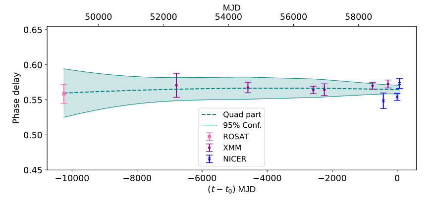
Figure 2: Residuals of the phase connection fit with the sinusoidal term removed. Each point corresponds to the average of the points in one of the panels in Figure 1.

3.2 Flux stability

The extensive coverage provided by the  observations offers, in principle, the possibility to constrain the variability of the X-ray emission along the orbit, as well as over long timescales. However, given the non-imaging nature of this instrument, this is complicated by two hindrances: the uncertainty in the background estimate and the presence of another variable source in the field of view. In fact, for this very soft source, most of the flux is at energies close to the lower limit of the  band, where the variable and high instrumental background (in our case even dominant with respect to the source) is difficult to model. Thus, the systematic uncertainties in the background hamper a precise measurement of the flux of our target. Moreover, the X-ray source 3XMM J064759.5$-$441941, is located at $\sim$ 1 arcmin from HD 49798, well within the field of view of . This is a main sequence M star with magnitude $G=12.88$, showing chromospheric activity (Martí et al., 2020). At energies above $\approx$0.4\text{\,}\mathrm{keV}$$ its flux is higher than that of our target. These concerns do not apply if we limit our study to the pulsed flux from RX J0648.0$-$4418. The total flux can then be inferred under the sole assumption that the pulsed fraction remains constant, as found in all the previous observations obtained with imaging X-ray instruments.

To this end, we corrected the times of arrival barycentering them with respect to the centre of the HD 49798/RX J0648.0$-$4418 system (in addition to the solar system) using the timing solution obtained in the previous section. We then took the counts in the $[0.2-0.55]\,$\mathrm{keV}$$ band and divided them in $9$ bins per orbit, so to have a sufficient statistics in each portion. We folded the resulting chunks of data with the parameters of Table 2 and fitted the pulse profiles with a constant plus a sinusoid. The amplitude of the sine then yields the pulsed fluxes shown in the upper panel of Figure 3 as a function of orbital phase. The lower panel shows the average value obtained by using all the NICER observations folded in 9 orbital bins.

Aside from the bin containing the eclipse at $\Phi_{\rm orb}=0.75$ (where the value of the pulsed flux is not shown because the pulsations are barely detectable or not visible at all), there is no conclusive evidence of a variation of the pulsed flux along the orbit, nor between the three time periods at hand. In fact, the fit of all data-points with a constant yields a pulsed flux of $0.141(3)\,$cts s^-1 with reduced $\chi^{2}=0.97$ and, in much the same way, the averaged pulsed fluxes in the three observation periods are compatible with a constant value.

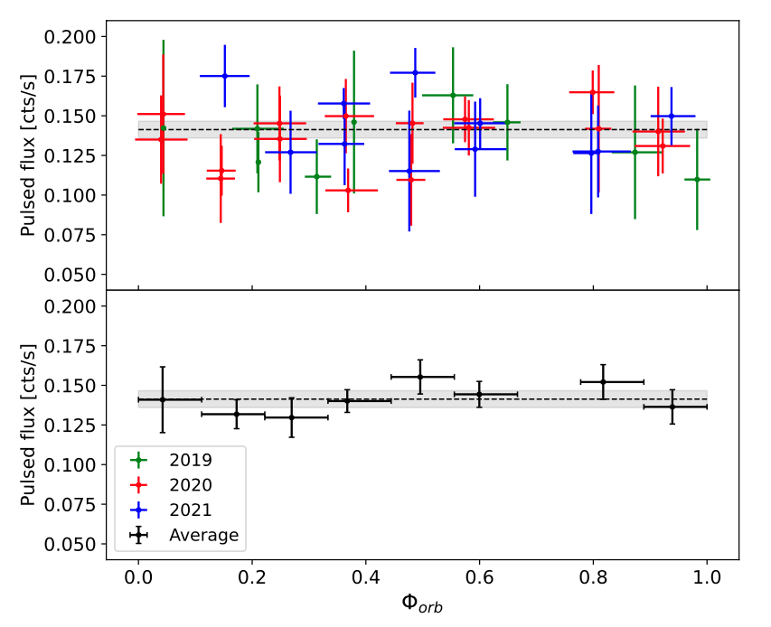
Figure 3: (Top panel): Pulsed flux in the 0.2–0.55 keV band as a function of the orbital phase, excluding the bins containing the eclipse at $\Phi_{\rm orb}=0.75$. Different colours denote the three observations (green: 2019, red: 2020, blue: 2021). (Bottom panel): Same, but averaging all the data in bins of 1/9th of orbital period. The dotted line is the fit with a constant value, with its $1\sigma$ uncertainty shaded in grey.

4 Discussion

The phase-connected timing solution derived in Section 3.1 indicates that RX J0648.0$-$4418 has continued to steadily spin-up also in the most recent years. The new value of $\dot{P}$ is $\sim$ 5% higher than the one reported in previous works (the difference is due to a mistake in the conversion of ROSAT times to TDB); at any rate, this does not affect the conclusion that such a high spin-up rate cannot be easily explained by accretion torques (Mereghetti et al., 2016). We found values of orbital parameters ($P_{\rm orb}$ and $t^{*}$) which are fully compatible with the more precise ones determined through optical observations (Schaffenroth et al., in preparation). In addition, thanks to the complete coverage of all orbital phases provided for the first time by the  data, we could refine the value of the projected semiaxis $a_{\rm X}\sin i=(9.60\pm 0.05)\,$lightsec. This, coupled with $a_{\rm opt}\sin i=(8.336\pm 0.009)$ lightsec (Schaffenroth, private communication), implies a mass ratio $q=M_{\rm opt}/M_{\rm X}=1.153\pm 0.006$.

Mereghetti et al. (2013) measured the duration of the X-ray eclipse as $(4311\pm 52$) s; the inclination of the system can be calculated from this value knowing the radius of HD 49798, $R_{\rm opt}$. Previous estimates used $R_{\rm opt}=(1.45\pm 0.25)\,$$\rm{R}_{\odot}$ (Kudritzki & Simon, 1978) and yielded an inclination in the range 79–84 deg. The downward revision of the distance (521 pc instead of 650 pc) and a more recent analysis of the optical/UV spectra, indicate instead $R_{\rm opt}=(1.08\pm 0.06)\,$$\rm{R}_{\odot}$ (Krtička et al., 2019). This implies an inclination $i=(84.5\pm 0.7)\,$deg. Finally, using the optical and X-ray mass functions, we can derive updated masses for the two components: $M_{\rm X}=(1.220\pm 0.008)$ $\rm{M}_{\odot}$ and $M_{\rm opt}=(1.41\pm 0.02)$ $\rm{M}_{\odot}$.

Under the assumption that the pulsed fraction of the X-ray emission is not changing over time, our results do not indicate a variation in the flux over the orbit nor between different observations. Note that our analysis, limited to the pulsed flux below 0.5 keV, is insensitive to possible variations in the subdominant power-law component, similar to that seen between the 2014 and 2020 XMM-Newton observations (Mereghetti et al., 2021).

4.1 On the nature of RX J0648.0$-$4418

Given the orbital parameters of the system, the Roche-lobe of HD 49798 has a radius of $\simeq$ 3 $\rm{R}_{\odot}$ (Eggleton, 1983), significantly larger than that of the hot subdwarf itself. Therefore, accretion cannot proceed through Roche-lobe overflow. Nevertheless, given the evidence that HD 49798 has a stellar wind with mass loss $\dot{M}_{\rm w}\simeq$2.1\text{\times}{10}^{-9}$\,$$\rm{M}_{\odot}$ yr^-1 and terminal velocity $v_{\infty}=1570$ km s^-1(Hamann et al., 1981; Krtička et al., 2019), it is natural to interpret the observed X-ray flux as the result of wind accretion, whereby only a small fraction, $\epsilon$, of the mass lost by the hot subdwarf is gravitationally captured by the compact object, without the formation of an accretion disk. In a simple Bondi-Hoyle accretion scenario (e.g. Shapiro & Teukolsky, 1986) $\epsilon$ can be estimated as

$$\epsilon=\left(\frac{R_{\rm A}}{2a}\right)^{2}$$ (2)

where $a$ is the orbital separation, $R_{\rm A}=2GM_{\rm X}/v^{2}$ is the accretion radius, and $v=(v_{\rm w}^{2}+v_{\rm orb}^{2})^{1/2}$ is the relative velocity between the wind and the compact object. For our system, $v_{\rm orb}\simeq 255$ km s^-1, thus we can take $v\sim v_{\rm w}$. Since the derived mass does not allow us to discriminate between a NS and a massive WD, in the following we discuss the evidences in favour or against each case.

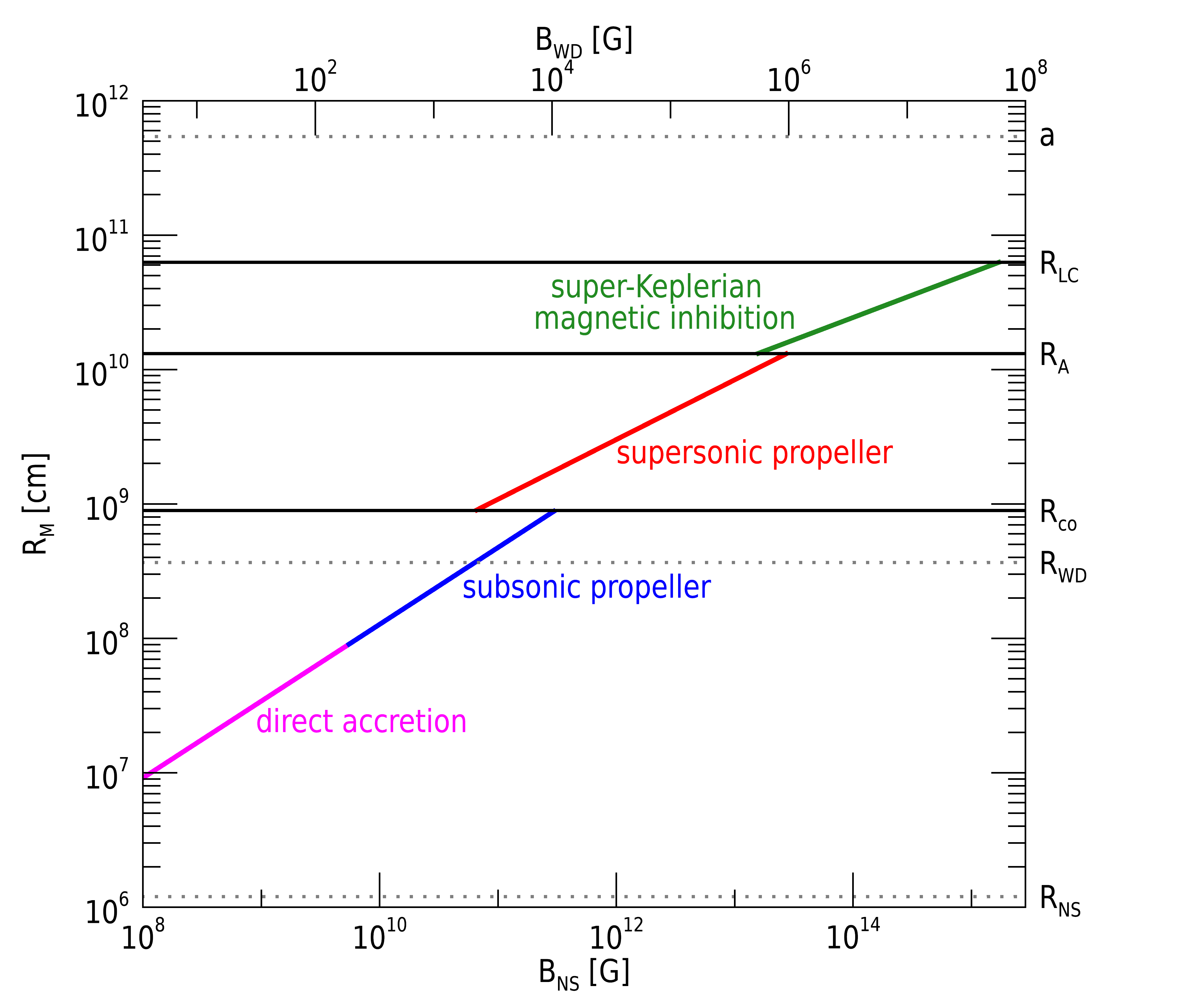
(a)

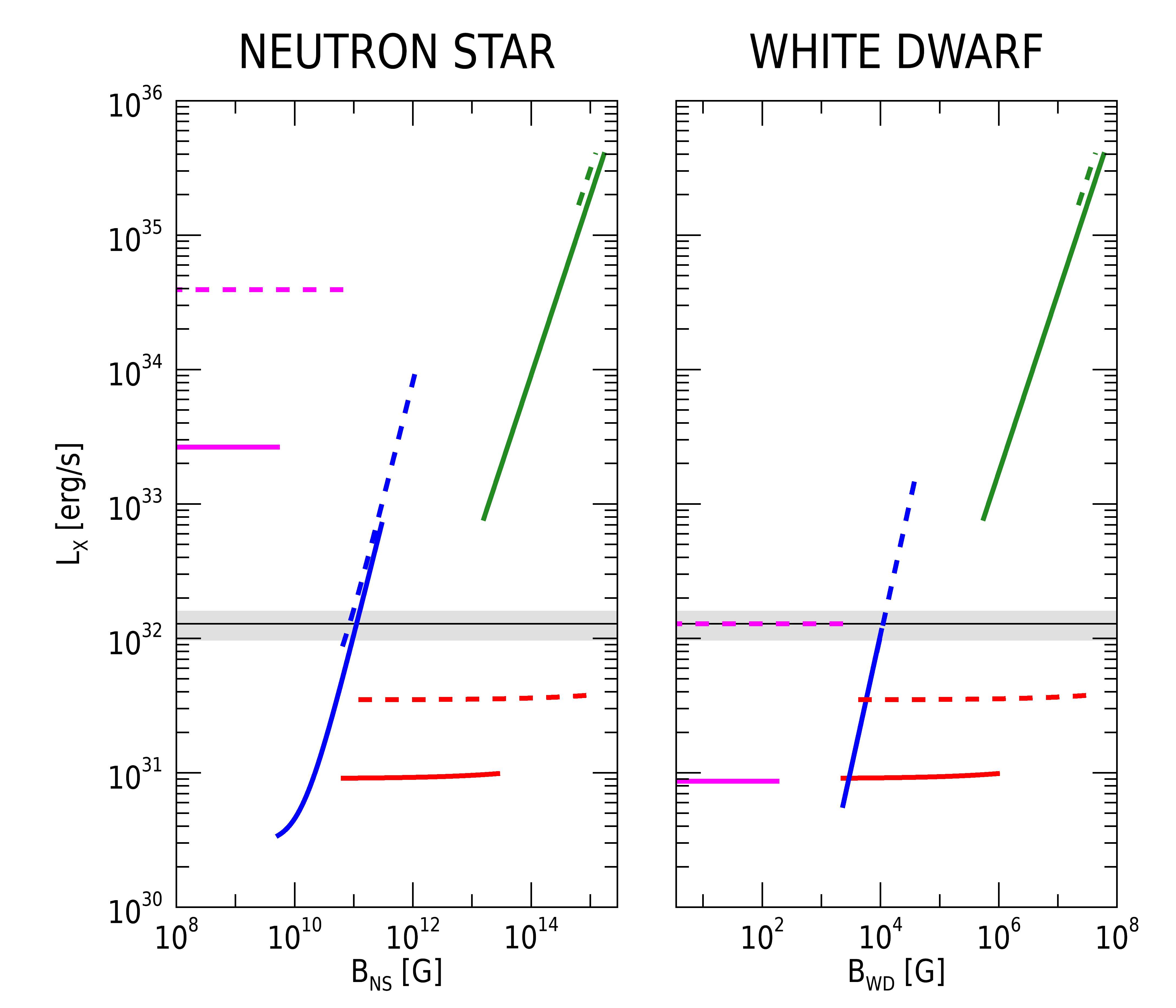
(b)

Figure 4: (a): Magnetospheric radius as a function of magnetic field for a NS (bottom scale) or a WD (top scale). The colors indicate the different regimes: super-Keplerian magnetic inhibition (green), supersonic propeller (red), subsonic propeller (blue), direct accretion (magenta). Other characteristic radii of the system are indicated by solid black lines: the light-cylinder radius $R_{\rm LC}=cP/2\pi\simeq 6.3\times 10^{10}$ cm, the accretion radius $R_{\rm A}=2GM_{\rm X}/v^{2}\simeq 1.3\times 10^{10}$ cm (for $v=1570$ km s^-1), and the corotation radius $R_{\rm co}=(GM_{\rm X}P^{2}/4\pi^{2})^{1/3}\simeq 9.0\times 10^{8}$ cm. The grey dotted lines indicate the orbital separation $a\simeq 5.4\times 10^{11}$ cm, the WD radius $R_{\rm WD}=3580$ km and the NS radius $R_{\rm NS}=12$ km. (b): The X-ray luminosities expected in the different regimes in the NS (left) and WD (right) cases (colours as in panel (a)) are compared to the observed value $L_{\rm X}=(1.3\pm 0.3)\times 10^{32}\,$erg s^-1 (solid black line, error as the grey horizontal band). Solid lines refer to $v=1570$ km s^-1, while the dashed lines to $v=800$ km s^-1 (see text).

4.1.1 Neutron star

In the aforementioned Bondi-Hoyle scenario, the expected luminosity for accretion onto the surface of a NS with radius $12$ km is

$$\begin{split}L_{\rm X}^{\rm NS}&=\frac{GM_{\rm X}}{R_{\rm NS}}\,\epsilon\dot{M}_{\rm w}\\ &\simeq$3\text{\times}{10}^{33}$\!\left(\frac{\dot{M}_{\rm w}}{2\times 10^{-9}\,\rm{M}_{\odot}/{\rm yr}}\right)\!\left(\frac{v_{\rm w}\vphantom{\dot{M}}}{1500~{}{\rm km/s}\vphantom{0^{9}}}\right)^{-4}\,{\rm erg\,s^{-1}},\end{split}$$ (3)

which is substantially larger than the observed value, ${L_{\rm X}=(1.3\pm 0.3)\times 10^{32}\,(d/521\text{\,}{\rm pc})^{2}}$ erg s^-1 (Mereghetti et al., 2016).

However, the accretion flow that reaches the surface of a NS can be drastically reduced by the effects related to the presence of the rotating magnetosphere. In particular, different regimes are determined by the relative position of four critical radii: the accretion radius $R_{\rm A}$, the corotation radius $R_{\rm co}=(GM_{\rm X}P^{2}/4\pi^{2})^{1/3}$, the light-cylinder radius $R_{\rm LC}=cP/2\pi$ and the magnetospheric radius $R_{\rm M}$ (see, e.g., Lipunov, 1992). The value of $R_{\rm M}$ itself acquires a different functional dependence on the parameters of the system in the different regimes (e.g. Campana et al., 1998; Bozzo et al., 2008). Figure 4(a) displays the behaviour of $R_{\rm M}$ as a function of the magnetic field strength for the parameters of our system, in the accretion regimes that are compatible with them. In Figure 4(b) we compare the luminosity expected in the different regimes with the observed value (solid black line, error as the grey horizontal band). The magnetic fields have been computed assuming a dipolar configuration; solid lines refer to the terminal wind velocity $v=1570$ km s^-1, while the dashed lines to $v=800$ km s^-1.

For NS magnetic fields above $\sim$ $10^{13}$ G, the magnetospheric radius is larger than $R_{\rm A}$, resulting in a super-Keplerian magnetic inhibition of the accretion. The wind is thus shocked at $R_{\rm M}$, where the magnetosphere is locally super-Keplerian and supersonic, and the gas kinetic energy is converted into thermal energy. The interaction between the NS magnetic field and matter at $R_{\rm M}$ results in the dissipation of rotational energy and NS spin-down, contrary to what is observed. Furthermore, the corresponding luminosity (green solid line in Figure 4(b)) would be much higher than the observed value.

For lower fields, $5\times 10^{9}\,\text{G}\lesssim B_{\rm NS}\lesssim 10^{13}$ G, $R_{\rm M}$ becomes smaller than $R_{\rm A}$, and the gravitationally captured matter is expected to form a nearly spherically symmetric and stationary configuration between these two radii (Davies & Pringle, 1981). If $R_{\rm M}>R_{\rm co}$ (supersonic propeller, red solid lines) a spin-down is still expected, while if $R_{\rm M}<R_{\rm co}$ (subsonic propeller, blue solid lines) a fraction of the inflowing matter can accrete onto the NS, due to the Kelvin-Helmoltz instability (Burnard et al., 1983). Using equations 7 and 21 of Bozzo et al. (2008) a lower limit on this mass inflow rate can be given as

$$\dot{M}_{\rm KH}\simeq 1.1\times 10^{-14}\!\left(\frac{\epsilon\dot{M}_{\rm w}}{3.1\times 10^{-13}\,\rm{M}_{\odot}/{\rm yr}}\right)^{1/7}\!\left(\frac{B_{\rm NS}\vphantom{\dot{M}}}{10^{11}\,{\rm G}\vphantom{0^{9}}}\right)^{12/7}\,{\rm\rm{M}_{\odot}/yr}.$$ (4)

With this reduced accretion rate, equation LABEL:eq:LNS yields a luminosity that is consistent with the observed one for $B\sim 10^{11}$ G. In this scenario, however, the observed spin-up rate can be barely explained. In fact, under the most optimistic assumption for the accreted angular momentum, i.e. that of matter in a Keplerian orbit at $R_{\rm M}$, the expected spin-up rate would be $\simeq 3\times 10^{-17}$ Hz s^-1 (for the above $B$ value and a moment of inertia $I_{\rm NS}=${10}^{45}$\,$g cm²). Nevertheless, the hypothesis of Keplerian rotation at $R_{\rm M}$ is unrealistic, since the angular momentum of the wind matter captured at $R_{\rm A}$, of the order of $\pi R_{\rm A}^{2}/2P_{\rm orb}$ (Frank et al., 2002), implies a circularization radius much smaller than $R_{M}$ for any reasonable wind velocity; therefore, the actual $\dot{\nu}$ is expected to be significantly lower.

For even lower magnetic fields, $\lesssim 5\times 10^{9}\,$G, the system would be in the regime described by equation LABEL:eq:LNS, which, as discussed above, predicts a luminosity much larger than the observed one (magenta solid lines in Figure 4).

In conclusion, even considering the interaction between the stellar wind of HD 49798 and the magnetic field of RX J0648.0$-$4418 under different regimes, it is quite difficult to explain the observed X-ray luminosity and spin-up rate.

At any rate, another element disfavouring the NS hypothesis is that the thermally emitting component has a very large emitting area, radius $\sim$ 40 km in the case of a blackbody model. This value can only increase by a factor 4–9 when more realistic magnetised atmosphere emission models are applied (see e.g. Ho et al., 2008). These dimensions are clearly not compatible with the size of a NS, nor with the idea that the emitting area is located at the edge of the magnetosphere, as this would not account for the large pulsed fraction ($\sim$ 60% below 0.5 keV).

4.1.2 White dwarf

As the luminosity from equation LABEL:eq:LNS depends on the radius of the compact object, in case RX J0648.0$-$4418 is a WD we are faced with the opposite problem. In fact, for $R_{\rm WD}=$3580\text{\,}\mathrm{km}$$, computed with the analytic mass-radius relation by Nauenberg (1972), the luminosity $L_{\rm X}^{\rm WD}\simeq$1\text{\times}{10}^{31}\text{\,}\mathrm{erg}\text{\,}{\mathrm{s}}^{-1}$$ is one order of magnitude below the observed one.

However, the luminosity has quite a strong dependence on the wind velocity, $L_{\rm X}\propto v_{\rm w}^{-4}$. Therefore, a comparatively small reduction of $v_{\rm w}$ can increase significantly the rate of accreted matter and hence the total luminosity; in our case, a wind velocity of about 800 km s^-1 would be required in order to reproduce the observed luminosity (magenta dashed line in the right panel of Figure 4(b)). Indeed, a viable mechanism that could reduce the wind velocity is its photo-ionisation by the X-rays emitted from the WD (Krtička et al., 2018). This mechanism is at work in luminous X-ray sources accreting from the strong winds of massive stars (e.g. Stevens, 1991, and references therein). It would be interesting to explore this possibility with a self-consistent model, taking into account the peculiar composition of the wind from HD 49798 and the way it is influenced by the X-ray emission from RX J0648.0$-$4418.

Even though a mass of $M_{\rm X}=(1.220\pm 0.008)$ $\rm{M}_{\odot}$ is quite high within the known population of WDs (e.g. McCleery et al., 2020), this value, coupled with the fast spin, is coherent with WD structure theory. In fact, for the period at hand, the mass lower limit imposed by the centrifugal mass-shredding condition is $M\gtrsim 1\,\rm{M}_{\odot}$ (see, e.g., fig. 2 of Otoniel et al., 2021). The high WD mass has also interesting implications for the future evolution of this system which might lead to a type Ia supernova (Wang & Han, 2010) or to the formation of a NS through accretion-induced collapse (Brooks et al., 2017).

5 Conclusions

Our new  observations of HD 49798/RX J0648.0$-$4418 indicate that the compact object in this unique binary has continued its steady spin-up without evidence for long term and/or orbital variations in the X-ray flux. We also derived new and more accurate values for the system inclination and for the masses of the two components (Table 2), which supersede those first reported in Mereghetti et al. (2009).

We thoroughly reexamined the possibility that this system contains a NS, but we could not find a satisfactory scenario able to reproduce at the same time the observed X-ray luminosity, spin-up rate, high pulsed fraction, and large emitting area of the thermal emission.

The possibility of a WD seems more promising because the spin-up can be accounted for, regardless of the accretion status, by the contraction mechanism proposed by Popov et al. (2018), and there is at least a plausible mechanism, i.e. photo-ionisation of the subdwarf wind, that could increase the accretion rate in such a way to be consistent with the observed luminosity. The verification of this scenario deserves a more detailed investigation.

Funnelling of the accreted matter by a low magnetic field (${B_{\rm dip}\lesssim 1\,}$kG, and/or the presence of some higher multipoles near the surface) would then account for the formation of a hot spot, thus explaining the high pulsed fraction of the thermal component. The size of the emitting region can extend up to radii of $\sim$ 1000 km when WD atmosphere models are used in the fit (Mereghetti et al., 2021).

The high mass of the object $M_{\rm X}=(1.220\pm 0.008)$ $\rm{M}_{\odot}$ does not represent an issue in the WD framework: other WDs with similar or even higher mass are known (e.g. Williams et al., 2022, and references therein). Note however that, contrary to most other cases, the mass of RX J0648.0$-$4418 has been determined with a dynamical measurement thanks to the presence of X-ray pulsations that make this system equivalent to a double spectroscopic binary. Another remarkable aspect is its short spin period of $13.2$ s, about twice shorter than that of the next fastest rotating WD (Pelisoli et al., 2022).

Popov et al. (2018) estimated that there are between 25 and 500 systems similar to HD 49798/RX J0648.0$-$4418  in the Galaxy, but these numbers are subject to large uncertainties due to the poorly known properties of the common envelope evolutionary phases. The small distance and high Galactic latitude clearly facilitated the discovery of HD 49798/RX J0648.0$-$4418, but fainter and more absorbed systems in the Galactic plane might be detected with future X-ray observations.

Data availability

All the data used in this article are available in public archives.

References

- Bozzo et al. (2008) Bozzo E., Falanga M., Stella L., 2008, ApJ, 683, 1031
- Brooks et al. (2017) Brooks J., Kupfer T., Bildsten L., 2017, ApJ, 847, 78
- Burnard et al. (1983) Burnard D. J., Arons J., Lea S. M., 1983, ApJ, 266, 175
- Campana et al. (1998) Campana S., Colpi M., Mereghetti S., Stella L., Tavani M., 1998, A&A Rev., 8, 279
- Davies & Pringle (1981) Davies R. E., Pringle J. E., 1981, MNRAS, 196, 209
- Deng & Jin (2022) Deng Y., Jin S., 2022, Universe, 8, 360
- Eggleton (1983) Eggleton P. P., 1983, ApJ, 268, 368
- Frank et al. (2002) Frank J., King A., Raine D. J., 2002, Accretion Power in Astrophysics (3rd ed.)
- Gaia Collaboration et al. (2021) Gaia Collaboration et al., 2021, A&A, 649, A1
- Gendreau et al. (2016) Gendreau K. C., et al., 2016, in den Herder J.-W. A., Takahashi T., Bautz M., eds, Society of Photo-Optical Instrumentation Engineers (SPIE) Conference Series Vol. 9905, Space Telescopes and Instrumentation 2016: Ultraviolet to Gamma Ray. p. 99051H, doi:10.1117/12.2231304
- Hamann et al. (1981) Hamann W. R., Gruschinske J., Kudritzki R. P., Simon K. P., 1981, A&A, 104, 249
- Ho et al. (2008) Ho W. C. G., Potekhin A. Y., Chabrier G., 2008, ApJS, 178, 102
- Iben & Tutukov (1985) Iben I. J., Tutukov A. V., 1985, ApJS, 58, 661
- Iben & Tutukov (1994) Iben Icko J., Tutukov A. V., 1994, ApJ, 431, 264
- Ikhsanov (2001) Ikhsanov N. R., 2001, A&A, 375, 944
- Israel et al. (1997) Israel G. L., Stella L., Angelini L., White N. E., Kallman T. R., Giommi P., Treves A., 1997, ApJ, 474, L53
- Krtička et al. (2018) Krtička J., Kubát J., Krtičková I., 2018, A&A, 620, A150
- Krtička et al. (2019) Krtička J., Janík J., Krtičková I., Mereghetti S., Pintore F., Németh P., Kubát J., Vučković M., 2019, A&A, 631, A75
- Kudritzki & Simon (1978) Kudritzki R. P., Simon K. P., 1978, A&A, 70, 653
- Lipunov (1992) Lipunov V. M., 1992, Astrophysics of Neutron Stars
- Martí et al. (2020) Martí J., Sánchez-Ayaso E., Luque-Escamilla P. L., Paredes J. M., Bosch-Ramon V., Corbet R. H. D., 2020, MNRAS, 492, 4291
- McCleery et al. (2020) McCleery J., et al., 2020, Monthly Notices of the Royal Astronomical Society, 499, 1890
- Mereghetti et al. (2009) Mereghetti S., Tiengo A., Esposito P., La Palombara N., Israel G. L., Stella L., 2009, Science, 325, 1222
- Mereghetti et al. (2013) Mereghetti S., La Palombara N., Tiengo A., Sartore N., Esposito P., Israel G. L., Stella L., 2013, A&A, 553, A46
- Mereghetti et al. (2016) Mereghetti S., Pintore F., Esposito P., La Palombara N., Tiengo A., Israel G. L., Stella L., 2016, MNRAS, 458, 3523
- Mereghetti et al. (2021) Mereghetti S., et al., 2021, MNRAS, 504, 920
- Nauenberg (1972) Nauenberg M., 1972, ApJ, 175, 417
- Otoniel et al. (2021) Otoniel E., Coelho J. G., Nunes S. P., Malheiro M., Weber F., 2021, A&A, 656, A77
- Pelisoli et al. (2022) Pelisoli I., et al., 2022, MNRAS, 509, L31
- Popov et al. (2018) Popov S. B., Mereghetti S., Blinnikov S. I., Kuranov A. G., Yungelson L. R., 2018, MNRAS, 474, 2750
- Shapiro & Teukolsky (1986) Shapiro S. L., Teukolsky S. A., 1986, Black Holes, White Dwarfs and Neutron Stars: The Physics of Compact Objects
- Stevens (1991) Stevens I. R., 1991, ApJ, 379, 310
- Thackeray (1970) Thackeray A. D., 1970, MNRAS, 150, 215
- Wang & Han (2010) Wang B., Han Z.-W., 2010, Research in Astronomy and Astrophysics, 10, 681
- Wang et al. (2014) Wang B., Meng X., Liu D. D., Liu Z. W., Han Z., 2014, ApJ, 794, L28
- Williams et al. (2022) Williams K. A., Hermes J. J., Vanderbosch Z. P., 2022, AJ, 164, 131
- Yungelson & Tutukov (2005) Yungelson L. R., Tutukov A. V., 2005, Astronomy Reports, 49, 871