Tempered geometric stable distributions and processes

Abstract

We introduce a notion of geometric tempering using exponentially-dampened Mittag-Leffler tempering functions and closely investigate the univariate case. Characteristic exponents and cumulants are calculated, as well as spectral densities. Absolute continuity relations are shown, and short and long time scaling limits of the associated Lévy processes analyzed.

Keywords: Tempered stable distributions, geometric stable distributions, Lévy processes, Mittag-Leffler function, generalized hypergeometric functions

1 Introduction

In physics and natural sciences, systems evolving according to Lévy stable distributions have long been observed (see Chechkin et al., (2008) for a survey). Modeling these phenomena as “Lévy flights/walks”, i.e., random processes with stationary independent stable increments has however the serious drawback of producing dynamic probabilistic representations with infinite variance, which is problematic both theoretically and in practice. In the seminal works of Mantegna and Stanley, (1994) and Koponen, (1995), Lévy a remedy was proposed by introducing a truncation procedure that, while inducing a minimal perturbation of the central part of distribution, impacted the tails in such a way as recovering finiteness of variance, and thus ultimately the Gaussian behavior of the process at large times. Since the observed convergence is very slow, for most practical purposes the Lévy stable empirical paradigm is robust to this modification. This idea proved be very successful and enjoyed a vast range of applications even outside physics, most notably in economics and finance: see Stanley, (2003) and the pioneering papers of Boyarchenko and Levendorskiĭ, (2000) and Carr et al., (2002) in option pricing. In particular Koponen’s idea of using a negative exponential cutoff function, yielding to a tractable analytic structure of the law, proved to be very consequential. Such procedure began to be known under the name of “tempering” of stable distributions, and with this word it was originally meant an exponential tilting of either the probability density function or the Lévy measure. Based on the remark that a negative exponential is a simple example of a completely monotone function, a general theory of tempering stable distributions using completely monotone functions is introduced by Rosiński, (2007), who shows that the properties of tempered laws can be fully described using characteristic measures (“spectral measures”). Specific parametric examples include the $p$-tempered stable law of Grabchak, (2016), the generalized tempered stable process of Rosiński and Sinclair, (2010), the modified and KR tempered stable laws in Kim et al., 2009a ; Kim et al., 2009b . Other possible choices of tempering functions and related distributions are explored in Terdik and Woyczynski, (2006).

In this work we introduce a novel class of tempered distributions, using as a tempering function an exponentially dampened negative Mittag-Leffler function. The Mittag-Leffler function is defined as

$$E_{\alpha}(z)=\sum_{k=0}^{\infty}\frac{z^{k}}{\Gamma(k+\alpha)},\qquad z\in\mathbb{C},\quad\alpha\in(0,1]$$ (1.1)

where $\Gamma$ stands for the Euler’s gamma function. For $r>0$ we thus consider distributions whose Lévy measures are given in polar coordinates, and with radial part of the form

$$\frac{e^{-\theta r}E_{\alpha}(-\lambda r^{\alpha})}{r^{1+\gamma}}dr,\>\quad r,\lambda,\theta>0,\,\alpha\in(0,1),\,\gamma\in(0,1).$$ (1.2)

In the above we see combined a stable inverse-power component, a classic exponential tempering function, and a negative Mittag-Leffler factor. The latter is a type of generalized exponential function with rapid decay around zero and power law tails.

The genesis of the proposed distribution can be retraced in the concept of geometric stability, introduced in Klebanov et al., (1985), answering the problem of finding a class of random variables which are infinitely-divisible under random geometric summation. A geometric stable law $X$ can be defined as an infinitely divisible distribution whose characteristic exponent $\psi_{X}$ can be written as a log-transform of a stable characteristic exponent $\psi_{Z}$ i.e.

$$\psi_{X}(z)=\log\left(1+\psi_{Z}(z)\right)$$ (1.3)

for some stable distribution $Z$. Theory and applications are developed by, among the others, Klebanov et al., (1985), Lin, (1998), Sandhya and Pillai, (1999), Mittnik and Rachev, (1991), Kozubowski and Rachev, (1999), Kozubowski and Podgórski, (2001). Known probability distributions such as the Laplace distribution and Pillai, (1990) Mittag-Leffler law are included in this class. Convolutions of geometric laws lead to the Linnik distribution (Linnik, (1963), Pakes, (1998), Christoph and Schreiber, (2001)) and the Erlang/gamma distribution as special cases. Tempered versions of the positive Linnik law (TPL) have been considered in Barabesi et al., 2016a Barabesi et al., 2016b and Torricelli et al., (2022). These are obtained by replacing the stable law $Z$ in (1.3) with a positive exponentially tempered stable variable. This makes it possible to introduce a notion of tempered geometric stability on the full space, by assuming a TPL for the radial part and then combining it with a finite measure on the unit sphere. We call these laws tempered geometric stable (TGS) distributions. As it turns out the Lévy measure of a TPL distribution constructed coincide with the mixed exponential/Mittag-Leffler in (1.2) when $\gamma=0$. Reverting to (1.2) in its full generality, i.e. considering instead an exponent $\gamma\in(0,2)$ at the denominator, determines what we call a generalized tempered geometric tempered stable law (GTGS), the general object of investigation of this study.

With regards to applications, the main motivation to study geometric tempering comes from economics and finance. A large number of independent statistical studies around the turn of the century (e.g. Lux, (1996), Longin, (1996), Gopikrishnan et al., (1998), Plerou et al., (1999), Gopikrishnan et al., (1999)) have reported strong evidence of power law decay (and scaling) of market returns which survive even at long lags, and with typical Pareto exponents of about 3. Therefore, according to these estimates, the existence of the variance in financial data is not called into question, while existence of higher moments remains a more delicate issue. It would then seem appropriate to seek dynamic return models whose distributions is of stable type in its central part and exhibits heavy law tails at longer lags, albeit with finite variance, and hence retaining Gaussian limiting properties. Bringing these features together is not easy. As argued in Chechkin et al., (2008) and Stanley, (2003), abrupt density truncation, or exponential tempering as proposed respectively by Mantegna and Stanley, (1994) and Koponen, (1995), determine too much of a sharp cutoff and do not maintain the power law decay for all the orders of magnitude for which it is observed in the empirical data, typically ranging from milliseconds to several days. One possible solution is proposed in Sokolov et al., (2004), where truncation is achieved by means of a model whose density function solves a Fokker-Planck equation of fractional order. In contrast, in the present work we show how to obtain heavy tails with finite variance at arbitrary lags by tempering stable laws (and the associated Lévy processes) using as a truncation function the Mittag-Leffler function, which corresponds to the particular case $\theta=0$ in (1.2). As we shall see the purely probabilistic approach followed leads to tractable analytic formulae and transparent asymptotic relations.

In this work we find the characteristic exponents of GTGS laws, their TGS subcases, as well as those of their purely Mittag-Leffler tempered subcases, and discuss their analytical properties. Such exponents involve two interesting special functions, namely Dotsenko’s ${}_{2}R_{1}$ generalized hypergeometric function (Dotsenko, (1991), Virchenko et al., (2001)), and Lerch’s transcendent $\Phi$. We determine cumulants and spectral densities, as well as short and long time scaling limiting behavior. In particular, in the pure Mittag-Leffler case we observe that the large parameter scaling can follow a classic Gaussian limit, but can also converge to stable process, depending on the stability and Mittag-Leffler parameters. Moreover, we analyze the absolute continuity conditions of GTGS laws within their own class as well as with with respect to stable laws.

We review the basic notions needed and fix the notation in Section 2. In Section 3 GTGS distributions are introduced. Their characteristic functions and cumulants are discussed in Section 4. In Section 5 we analyze spectral measures, short and long time limits as well as absolute continuity properties. S In Section 6 we conclude and discuss possible developments.

2 Preliminaries

We begin by establishing the notation and recalling some concepts and notions required throughout the paper.

2.1 Infinitely divisible laws and Lévy processes

Throughout the paper we fix a filtered probability space $(\Omega,\mathcal{F},(\mathcal{F}_{t})_{t\geq 0},P)$ to which all the processes we mention are adapted. For a $d$-dimensional random variable $X$ on such space we denote by $\Psi_{X}:\mathbb{R}^{d}\rightarrow\mathbb{C}$ its characteristic function

$$\Psi_{X}(z)=E[e^{i\langle z,X\rangle}].$$ (2.1)

An infinitely-divisible (i.d.) random variable is fully characterized by its characteristic exponent $\psi_{X}(z)$ i.e, a function $\psi_{X}:D\subseteq\mathbb{R}^{d}\rightarrow\mathbb{C}$ such that

$$\Psi_{X}(z):=E[e^{i\langle z,X\rangle}]=e^{t\psi_{X}(z)}.$$ (2.2)

The exponent $\psi_{X}$ can be written in terms of a characteristic triplet $(\mu,\Sigma,\nu)$ with $\mu\in\mathbb{R}^{d}$, $\Sigma$ is a positive definite $d\times d$ matrix, $\nu$ is a measure on $\mathbb{R}^{d}$ such that $\nu(0)=0$, $\int_{\mathbb{R}^{d}}(|x|^{2}\wedge 1)dx<\infty$, with $|\cdot|$ indicating the Euclidean norm, and

$$\psi_{X}(z)=i\langle z,\mu\rangle-\langle z,\Sigma z\rangle/2+\int_{\mathbb{R}^{d}}\left(e^{i\langle z,x\rangle}-1-i\langle z,x\rangle\mathds{1}_{\{|x|<1\}}\right)\nu(dx)$$ (2.3)

where $\langle\cdot,\cdot\rangle$ is the standard inner product on $\mathbb{R}^{d}$. The measure $\nu$ is called the Lévy measure. When $\nu$ is absolutely continuous its corresponding density is the Lévy density. The function $x\mathds{1}_{\{|x|<1\}}$ ensures the convergence of the integral in 0, and is called a truncation function. Equation (2.3) goes under the name of Lévy-Khintchine representation. When $d=1$ and $X$ is a positively supported i.d. random variable then one can also use the Laplace exponent $\phi$, defined to be the complex valued function such that

$$L_{X}(z):=E[e^{-sX}]=e^{-\phi_{X}(s)},\qquad s>0$$ (2.4)

with

$$\phi_{X}(s)=a+bs+\int_{\mathbb{R}_{+}}(1-e^{-sx})\nu(dx)$$ (2.5)

for some triplet $(a,b,\nu)$, with $a,b\geq 0$ and a positively-supported Lévy measure $\nu$ satisfying $\int_{\mathbb{R}_{+}}(x\wedge 1)\nu(dx)<\infty$. One generic function $f$ enjoying representation (2.5) is called a Bernstein function. A Bernstein function $f\in C^{\infty}(\mathbb{R}_{+})$ is equivalently characterized by the property of being such that, for all $n\in\mathbb{N}_{0}$

$$(-1)^{n-1}f^{(n)}(x)\geq 0.$$ (2.6)

indicating the $n$-th derivative with the parenthetical exponent. A completely monotone function on $\mathbb{R}_{+}$ is a function of class $C^{\infty}$ such that $f^{\prime}$ is a Bernstein function. A classic reference for Bernstein functions is Schilling et al., (2012).

A real-valued r.v. $X$ i.d. is said to be self-decomposable (s.d.) if for all $\alpha\in(0,1)$ can be written in law as $X=\alpha X+R_{\alpha}$, for some r.v. $R_{\alpha}$ independent of $X$. Equivalently, a real valued s.d. distribution is characterized by the property that its Lévy measure is absolutely continuous and its density $v(x)$ writes as $v(x)=k(x)/|x|$, with $k(x)$ a function increasing on $\mathbb{R}_{-}$ and decreasing on $\mathbb{R}_{+}$. The function $k$ is called the canonical density of $X$.

A Lévy process $X=(X_{t})_{t\geq 0}$ on $\mathbb{R}^{d}$ is a stochastically continuous process with independent and stationary increments. For a Lévy process $X$, $X_{t}$ is i.d. for all $t>0$. Conversely, given an i.d. random variable $\mathcal{X}$ there exists a unique in law Lévy process $X$ such that $X_{1}=\mathcal{X}$ (Sato, (1999), Theorem 7.10). The characteristic exponent $\psi_{X}$ of a Lévy process $X$ is by definition $\psi_{X_{1}}$. With abuse of terminology we shall refer to a Lévy process by the name of its unit time law.

2.2 Stable and tempered stable laws and processes

A stable S${}_{\alpha}(\lambda,\beta;\mu)$ r.v. on $\mathbb{R}$, with $\alpha\in(0,2]$, $\mu\in\mathbb{R},\lambda>0$ is one such that the equality $\Psi_{X}(z)^{\alpha}=\Psi_{X}(z^{1/\alpha})e^{iz\mu}$ holds. If $\mu=0$ the r.v. is said to be strictly stable. The r.v. $X$ is i.d. with characteristic exponent

$$\psi_{X}(z)=\left\{\begin{array}[]{cc}-\lambda|z|^{\alpha}\left(1-i\beta\mbox{sgn}(z)\tan(\pi\alpha/2)\right)+iz\mu&\mbox{ for }\alpha\neq 1\\ -\lambda|z|\left(1+i\beta\frac{2}{\pi}\mbox{sgn}(z)\log|z|\right)+iz\mu&\mbox{ for }\alpha=1\end{array}\right.$$ (2.7)

where $\beta\in[-1,1]$, $z\in\mathbb{R}$. For $\beta=0$ the distribution is symmetric, for $\beta=\pm 1$ totally skewed respectively to the right and left. Stable laws are i.d., and an $\alpha$-stable Lévy process $X=(X_{t})_{t\geq 0}$ is one for which $X_{1}$ is stable (equiv. $X_{t}$ is stable for all $t$).

On $\mathbb{R}^{d}$, $d\geq 1$, it is instead easier to define a stable process by means of its Lévy triplet $(\mu,0,\nu)$ where for $B\in\mathcal{B}(\mathbb{R}^{d}\setminus\{0\})$ we have the following polar representation

$$\nu(B)=\int_{S^{d-1}}\sigma(du)\int_{\mathbb{R}_{+}}\mathds{1}_{B}(ru)\frac{dr}{r^{1+\alpha}}$$ (2.8)

with $S^{d}$ indicating the $d$-dimensional sphere. We denote the class of $\alpha$-stable distributions on $\mathbb{R}^{d}$ with S${}_{\alpha}(\sigma,\mu)$. On $\mathbb{R}$, sometimes cases with different stability indices for the two distinct points in $S^{0}$ are taken into account, when the Lévy measure $\nu$ has an absolutely continuous density $v(x)$ of the form

$$v(x)=\frac{\delta_{+}}{x^{1+\alpha_{+}}}\mathds{1}_{\{x>0\}}+\frac{\delta_{-}}{|x|^{1+\alpha_{-}}}\mathds{1}_{\{x<0\}},$$ (2.9)

with $\alpha_{+},\alpha_{-}\in(0,2]$. When $\alpha_{+}=\alpha_{-}$ the constants $\delta_{+}$ and $\delta_{-}$ are related to the classical parametrization (2.7) by $\lambda=\delta_{+}+\delta_{-}$ and $\beta=(\delta_{+}-\delta_{-})/(\delta_{+}+\delta_{-})$. In this case we denote the class of the stable distributions by S${}_{{\bm{\alpha}}}({\bm{\delta}},\mu)$, with ${\bm{\alpha}}=(\alpha_{+},\alpha_{-})\in(0,2]\times(0,2]$, ${\bm{\delta}}=(\delta_{+},\delta_{-})\in\mathbb{R}^{2}_{+}$, $\mu\in\mathbb{R}$. For a detailed survey on stable distribution see Sato, (1999), Chapter 3.

A (classical) tempered stable distribution is an i.d. distribution with Lévy measure $\nu$ given by

$$\nu(dx)=\delta_{+}\frac{e^{-\theta_{+}}x}{x^{1+\alpha_{+}}}\mathds{1}_{\{x>0\}}+\delta_{-}\frac{e^{-\theta_{-}|x|}}{|x|^{1+\alpha_{-}}}\mathds{1}_{\{x<0\}}$$ (2.10)

for $\alpha_{+},\alpha_{-}\in(0,2]$, $\delta_{+},\delta_{-}\geq 0$, see e.g. Koponen, (1995), Boyarchenko and Levendorskiĭ, (2000), Carr et al., (2002) for applications, and Küchler and Tappe, (2013) for a theoretical analysis. We shall use the notation CTS${}_{{\bm{\alpha}}}({\bm{\theta}},{\bm{\delta}};\mu)$ with ${\bm{\alpha}}=(\alpha_{+},\alpha_{-})\in\mathbb{(}0,2]\times(0,2]$, ${\bm{\theta}}=(\theta_{+},\theta_{-})\in\mathbb{R}^{2}_{+}$, ${\bm{\delta}}=(\delta_{+},\delta_{-})\in\mathbb{R}^{2}_{+},\mu\in\mathbb{R}$. Special cases, other than the stable distributions when $\theta_{\pm}=0$, include the bilateral Gamma BG$({\bm{\theta}},{\bm{\delta}})$ laws (e.g. Küchler and Tappe, (2008)) is obtained for ${\bm{\alpha}}=0$, and the ordinary positively-supported gamma G$(\theta,\delta)$ law, obtained for $\alpha_{+}=\alpha_{-}=\delta_{-}=0$.

A general approach to tempering stable laws is considered in Rosiński, (2007). Let $\sigma$ be a finite measure on $S^{d-1}$ and a function $q:\mathbb{R}_{+}\times S^{d-1}\rightarrow\mathbb{R}^{d}$, $(r,u)\mapsto q(r,u)$, completely monotone in $r$ for all $u$. Then for $\alpha\in(0,2]$ an $\alpha$ tempered stable process on $\mathbb{R}^{d}$ is one with Lévy triplet $(\mu,0,m)$ where $m$ is given in polar coordinates by

$$m(dr,du)=\frac{q(r,u)}{r^{1+\alpha}}{\sigma(du)}dr.$$ (2.11)

Since $q$ is completely monotone in the first variable, by the Bernstein Theorem (Schilling et al., (2012), Theorem 1.4) there exists a family of probability measures $(Q_{u})_{u\in S^{d-1}}$ supported on $\mathbb{R}_{+}$ for which

$$q(r,u)=\int_{0}^{\infty}e^{-rs}Q_{u}(ds).$$ (2.12)

Therefore for $B\in\mathcal{B}(\mathbb{R}^{d}\setminus\{0\})$ we can introduce two measures $Q$ and $R$ respectively by

$$Q(B)=\int_{S^{d-1}}\sigma(du)\int_{\mathbb{R}_{+}}\mathds{1}_{B}(ru)Q_{u}(dr)$$ (2.13)

and

$$R(B)=\int_{\mathbb{R}^{d}}\mathds{1}_{B}\left(\frac{x}{\|x\|^{2}}\right)\|x\|^{\alpha}Q(dx).$$ (2.14)

It turns out that $R$ and $Q$ are dual in the sense that

$$Q(B)=\int_{\mathbb{R}^{d}}\mathds{1}_{B}\left(\frac{x}{\|x\|^{2}}\right)\|x\|^{\alpha}R(dx).$$ (2.15)

We call $Q$ the spectral measure and $R$ the Rosińsky measure. A given tempered $\alpha$ stable distribution is fully characterized by its measures $Q$ or $R$, and a drift vector $\xi\in\mathbb{R}^{d}$. The measure $Q$ is useful for computer simulations (Cohen and Rosiński, (2007)), whereas $R$ is pivotal to describe the analytical properties of the law.

With abuse of notation, we denote the class of tempered stable distributions in the sense of Rosińsky by TS${}_{\gamma}(\sigma,q,\mu)$, TS${}_{\gamma}(Q,\mu)$, or TS${}_{\gamma}(R,\mu)$, which covers all the different specifications illustrated above.

2.3 Geometric stability and tempered geometric stability

Geometric stable (GS) laws were introduced by Klebanov et al., (1985) as a solution to the problem of characterizing i.d. laws whose infinite divisibility property holds true with respect to geometric summation. A geometric strictly stable law $X$ on $\mathbb{R}^{d}$ is one such that

$$\psi_{X}(z)=\log\left(1+\psi_{Z}(z)\right)$$ (2.16)

is the characteristic exponent of some stable r.v. $Z$ on $\mathbb{R}^{d}$. In the case $d=1$ and when $\beta=0$ in (2.7) we have the symmetric law with Laplace exponent

$$\phi_{X}(z)=\delta\log\left({1+\lambda|z|^{\alpha}}\right),\qquad\delta,\lambda>0,\quad\alpha\in(0,2],\quad z>0.$$ (2.17)

The arising probability distribution is often called the Linnik distribution. When $\alpha=2$, $\delta=\lambda=1$ this reduces to the well-known Laplace distribution.

Geometric stable processes and their applications have been studied in e.g. Mittnik and Rachev, (1991), Šikić et al., (2006) Kozubowski and Rachev, (1999), Kozubowski et al., (1999), Kotz et al., (2001), Kozubowski and Podgórski, (2001). Positively-supported Linnik PL$(\alpha,\lambda,\delta)$ laws can be seen as extension of the Mittag-Leffler ML$(\alpha,\lambda)$ law introduced in Pillai, (1990). We have, for the Lévy measure of a PL$(\alpha,\lambda,\delta)$ r.v. $X$ the Lévy density

$$v_{X}(x)=\frac{\delta}{x}E_{\alpha}\left(-\frac{x^{\alpha}}{\lambda}\right),\qquad x>0,\quad\alpha\in(0,1)$$ (2.18)

and PL$(\alpha,\lambda,1)\equiv$ ML$(\alpha,\lambda)$.

In Barabesi et al., 2016b a tempered version of the Linnik positive laws, denoted TPL$(\alpha,\lambda,\theta,\delta)$ was investigated, and their associated processes later studied in Kumar et al., (2019) and Torricelli et al., (2022). The resulting operation leads to the Laplace transform

$$\phi_{X}(s)={\delta}\log\left({1+\lambda((\theta+s)^{\alpha}-\theta^{\alpha})}\right)$$ (2.19)

Recalling that the Laplace exponent of a CTS${}^{+}_{\alpha}(\theta,\lambda;0)$ law is $\lambda((\theta+s)^{\alpha}-\theta^{\alpha})$, we see that (2.19) is equivalent to requiring that (2.16) now holds for a Laplace exponent of some tempered stable positive law $Z$. The expression for the Lévy density is

$$v_{X}(x)=\delta\frac{e^{-\theta x}}{x}E_{\alpha}\left(\frac{\lambda\theta^{\alpha}-1}{\lambda}x^{\alpha}\right),\qquad x>0,\alpha\in(0,1).$$ (2.20)

TPL distributions seem to have first appeared in Meerschaert et al., (2011), Example 5.7, to describe the waiting times of a Poisson process subordinated to an inverse tempered stable subordinator (an increasing Lévy process). A closed form expression in terms of the three-parameter Mittag-Leffler function is also available for the p.d.f.. See Barabesi et al., 2016b and Torricelli et al., (2022) for details.

2.4 Special functions

We denote with $E_{a,b}^{c}(z)$, $z\in\mathbb{C}$, the Prabhakar, (1971) three-parameter Mittag-Leffler function given by

$$E_{a,b}^{c}(z)=\sum_{k=0}^{\infty}\frac{(c)_{k}z^{k}}{k!\Gamma(ak+b)},\qquad\text{Re}(a)>0,\quad\text{Re}(b)>0,\quad c,z\in\mathbb{C},$$ (2.21)

where $\Gamma(\cdot)$ is the Euler’s Gamma function and $(c)_{k}=\Gamma(c+k)/\Gamma(c)$ the Pochhammer symbol. The standard and two-parameter Mittag-Leffler functions $E_{a}$ and $E_{a,b}$ coincide with $E_{a,1}^{1}$ and $E_{a,b}^{1}$ respectively. All these functions are entire.

The following leading asymptotic order of the three-parameter Mittag-Leffler function (e.g. Garra and Garrappa, (2018)), as $x\in\mathbb{R}$, $x\rightarrow\infty$ will be useful

$$E_{a,ac}^{c}(-x^{a})\sim-c\frac{x^{-a(c+1)}}{\Gamma(-a)},\qquad a\in(0,1),\quad c>0$$ (2.22)

from which we can recover the well-known formula (e.g. Haubold et al., (2011))

$$E_{\alpha}(-x^{\alpha})\sim \frac{x^{-\alpha}}{\Gamma(1-\alpha)},\quad x\rightarrow\infty,\qquad\alpha\in(0,1).$$ (2.23)

From the definition it is also clear that

$$E_{\alpha}(-x^{\alpha})\sim 1-\frac{x^{\alpha}}{\Gamma(1+\alpha)}\sim\exp\left(-\frac{x^{\alpha}}{\Gamma(1+\alpha)}\right),\quad x\rightarrow 0.$$ (2.24)

See Haubold et al., (2011) or Gorenflo et al., (2020) for a comprehensive introduction on Mittag-Leffler functions.

The ${}_{2}R_{1}$ generalized hypergeometric Wright-type function studied by Dotsenko, (1991) and Virchenko et al., (2001), is given by for $\tau>0,a,b,c\in\mathbb{C},c\not\in\mathbb{Z}_{\leq 0}$

$$_{2}R_{1}(a,b,c,\tau;z)=\frac{\Gamma(c)}{\Gamma(b)}\sum_{k=0}^{\infty}\frac{(a)_{k}\Gamma(b+\tau k)}{\Gamma(c+\tau k)}\frac{z^{k}}{k!},\qquad\mbox{Re}(c-b-a)>0.$$ (2.25)

Under this assumptions the power series expansion above converges absolutely for $|z|\leq 1$, but the ${}_{2}R_{1}$ function can be continued analytically on $\mathbb{C}\setminus(1,\infty)$. For $|z|<1$, $|\text{Arg}(-z)|<\pi$ the expression of the continuation is given by e.g Kilbas et al., (2003). Notice that ${}_{2}R_{1}(a,b,c,1;z)=\,_{2}F_{1}(a,b,c;z)$, Gauss’ hypergeometric function, so that in particular ${}_{2}R_{1}(a,b,b,1;z)=(1-z)^{-a}$ . Furthermore, the generalized hypergeometric ${}_{2}R_{1}$ can be represented in terms of the normalized Fox-Wright (Wright, (1935)) function ${}_{p}\Psi^{*}_{q}$ as

$$_{2}R_{1}(a,b,c,\tau;z)=\,_{2}\Psi^{*}_{1}\left[\begin{array}[]{c c}(a,1)&(b,\tau)\\ (c,\tau)&\end{array};z\right].$$ (2.26)

See also Braaksma, (1963) and Karp and Prilepkina, (2020) for details on the analytic continuation of the ${}_{p}\Psi_{q}$ function.

The Lerch transcendent function $\Phi$ is defined as the convergent series

$$\Phi(z,s,a)=\sum_{k=0}^{\infty}\frac{z^{k}}{(a+k)^{s}},\qquad z,s\in\mathbb{C},|z|<1,a\notin\mathbb{Z}_{\leq 0}.$$ (2.27)

It relates to the Polilogarithm Li${}_{s}(z)$ through Li${}_{s}(z)/z=\Phi(z,s,1)$ and extends the Hurwitz/Riemann Zeta functions, in that $\zeta(s,a)=\Phi(1,s,a)$, $\zeta(s)=\Phi(1,s,0)$. Again, even though the series representation above is only valid for $|z|<1$, and for $|z|=1$ if Re$(s)>0$, analytic continuations are available, and have been recently studied (Ferreira et al., (2017)).

3 Geometric tempered stable distributions

In order to construct a multivariate geometric tempered stable distributions we follow the approach in Rosiński, (2007) of defining a Lévy measure in polar coordinates using a positive probability measure for the radial part and a measure $\sigma$ to move it along the unit sphere.

Let $d\geq 1$ and $\theta,\lambda:S^{d-1}\rightarrow\mathbb{R}_{+}$, $\alpha:S^{d-1}\rightarrow(0,1]$ continuous functions. Let the tempering function in (2.11) be given by

$$q(r,u;\alpha,\lambda,\theta)=e^{-\theta(u)r}E_{\alpha(u)}\left(-\lambda(u)r^{\alpha(u)}\right).$$ (3.1)

In order to avoid degeneracies, the following technical assumption is needed:

• either $\theta$, or both $\alpha$ and $\lambda$, are bounded away from zero.

To begin with one needs to show that (3.1) is a legitimate tempering function, and that this is so even in the case $\gamma=0$.

Proposition 1.

Let $\sigma(du)$ be a finite measure on $S^{d-1}$. For $\gamma\in(0,2)$ the function $q(r,u;\alpha,\lambda,\theta)$ is a tempering function in the sense of Rosiński, (2007). Furthermore, under assumption (B).

$$m_{0}(dr,du;\sigma,\alpha,\lambda,\theta):=\frac{q(r,u;\alpha,\lambda,\theta)}{r}\sigma(du)dr$$ (3.2)

is a Lévy measure. Therefore under the given conditions

$$m_{\gamma}(dr,du;\sigma,\alpha,\lambda,\theta):=\frac{q(r,u;\alpha,\lambda,\theta)}{r^{1+\gamma}}\sigma(du)dr$$ (3.3)

is a Lévy measure for all $\gamma\in[0,2)$.

Proof.

The exponential function is completely monotone for all $\theta<0$, and so is the function $E_{\alpha}(-\,\cdot)$ (Pollard, (1948)). Furthermore the function $x\rightarrow\lambda x^{\alpha}$, $\alpha\in(0,1)$ is positive with a completely monotone derivative, so that its composition with $E_{\alpha}(-\,\cdot)$ is also completely monotone. Therefore $q(\cdot,u)$ is completely monotone, it being a product of completely monotone functions (Schilling et al., (2012), Corollary 1.6), for all possible values of $u$. Observe also that $q(0+,u)=1$, for all $u$.

To complete the proof we only need to show that $\int_{\mathbb{R}^{d}}((ru)^{2}\wedge 1)m_{0}(dr,du)<\infty$, since for positive values of $\gamma$ this is a particular cases of Rosiński, (2007) analysis. From $\exp(\cdot),E_{\alpha}(-\,\cdot)\leq 1$ we have

$$\int_{S^{d-1}}\int_{0}^{1}r^{2}\frac{q(r,u;\alpha,\lambda,\theta)}{r}dr\sigma(du)<\sigma(S^{d-1})\int_{0}^{1}rdr<\infty$$ (3.4)

Also, by assumption (B) it follows that if $\theta_{*}=\min_{S^{d-1}}\theta(u)=0$ then both $\lambda_{*}=\min_{S^{d-1}}\lambda(u),$ and $\alpha_{*}=\min_{S^{d-1}}\alpha(u)$ are strictly positive. Then in view of (2.23) it follows

$$\int_{S^{d-1}}\int_{1}^{\infty}\frac{q(r,u;\alpha,\lambda,\theta)}{r}dr\sigma(du) <\sigma(S^{d-1})\int_{1}^{\infty}r^{-1}E_{\alpha_{*}}(-\lambda_{*}r^{\alpha_{*}})dr$$

$$\sim\frac{\sigma(S^{d-1})}{\lambda_{*}\Gamma(1-\alpha_{*})}\int_{1}^{\infty}r^{-1-\alpha_{*}}dr<\infty.$$ (3.5)

Similarly if $\lambda_{*},\alpha_{*}=0$ then $\theta_{*}>0$ whence

$$\int_{S^{d-1}}\int_{1}^{\infty}\frac{q(r,u;\alpha,\lambda,\theta)}{r}dr\sigma(du)<\sigma(S^{d-1})\int_{1}^{\infty}r^{-1}e^{-r\theta_{*}}dr<\infty.$$ (3.6)

∎

We can thus define a general $d$-dimensional GTGS variable as follows.

Definition 1.

Let $d\geq 1$, $\gamma\in[0,2)$, $\sigma(du)$ be a finite measure on $S^{d-1}$, and $\mu\in\mathbb{R}^{d}$. A generalized tempered geometric $\gamma$-stable distribution GTGS${}_{\gamma}(\sigma,\alpha,\lambda,\theta;\mu)$ on $\mathbb{R}^{d}$ is the i.d. distribution determined by the Lévy triplet $(\mu,0,m_{\gamma}(dr,du;\sigma,\alpha,\lambda,\theta))$. A tempered geometric stable distribution TGS$(\sigma,\alpha,\lambda,\theta;\mu)$ is a GTGS${}_{0}(\sigma,\alpha,\lambda,\theta;\mu)$ distribution.

When $\sigma(du)=\sigma du$, $\sigma>0$ and $\lambda,\theta,\alpha$ are constant functions, the GTGS distribution is rotationally-invariant (i.e. symmetric).

In this paper we will explore in detail the case $d=1$, which is easier being $S^{0}=\{-1,1\}$ and a great deal can be said on the analytic structure of the distributions. In such case the spherical measure reduces to

$$\sigma(du)=\delta_{+}\delta_{1}(du)+\delta_{-}\delta_{-1}(du)$$ (3.7)

for $\delta_{+},\delta_{-}\geq 0$ and $\delta_{x}$ is the Dirac delta measure concentrated in $x\in\mathbb{R}$. We have the following expression for the Lévy density, with $\alpha(u)=\alpha_{\pm}$, $\theta(u)=\theta_{\pm}$, $\lambda(u)=\lambda_{\pm}$

$$m_{\gamma}(dr,du;\sigma,\alpha,\lambda,\theta)=\delta_{+}\frac{e^{-\theta_{+}r}}{r^{1+\gamma}}E_{\alpha_{+}}(-\lambda_{+}\,r^{\alpha_{+}})dr\delta_{1}(du)+\delta_{-}\frac{e^{-\theta_{-}r}}{r^{1+\gamma}}E_{\alpha_{-}}(-\lambda_{-}\,r^{\alpha_{-}})dr\delta_{-1}(du).$$ (3.8)

One can easily extend this definition by assuming the stability indices for the negative and positive parts are not necessarily equal i.e. if $\gamma_{+}\neq,\gamma_{-}\in[0,2]$, using the vector notation

$${\bm{\alpha}} =(\alpha_{+},\alpha_{-})\in(0,1]\times(0,1],$$

$${\bm{\lambda}} =(\lambda_{+},\lambda_{-})\in(0,\infty)\times(0,\infty),$$

$${\bm{\theta}} =(\theta_{+},\theta_{-})\in[0,\infty)\times[0,\infty),$$ (3.9)

$${\bm{\delta}} =(\delta_{+},\delta_{-})\in[0,\infty)\times[0,\infty)\setminus\{(0,0)\},$$

$${\bm{\gamma}} =(\gamma_{+},\gamma_{-}),\in[0,2)\times[0,2)$$

in Cartesian coordinates we have the expression for the Lévy density

$$m_{{\bm{\gamma}}}(x;{\bm{\alpha}},{\bm{\lambda}},{\bm{\theta}},{\bm{\delta}})=\delta_{+}\frac{e^{-\theta_{+}x}}{x^{1+{\gamma_{+}}}}E_{\alpha_{+}}(-\lambda_{+}\,x^{\alpha_{+}})\mathds{1}_{\{x>0\}}+\delta_{-}\frac{e^{-\theta_{-}|x|}}{|x|^{1+\gamma_{-}}}E_{\alpha_{-}}(-\lambda_{-}\,|x|^{\alpha_{-}})\mathds{1}_{\{x<0\}}.$$ (3.10)

When the Lévy measure is symmetric, or it has positive/negative support we write respectively $m_{\gamma}(x;\alpha,\lambda,\theta,\delta)$, $m^{+}_{\gamma}(x;\alpha,\lambda,\theta,\delta)$, $m^{-}_{\gamma}(x;\alpha,\lambda,\theta,\delta)$, where the constants denote the only surviving value for each parameter vector. In these two latter instances the corresponding GTGS laws are said to be spectrally positive (resp. negative). It is important to recall the spectral positive/negativity is not the same as the corresponding probability laws being positively/negatively supported, although this equivalence holds true when $\gamma\in[0,1)$ and $\mu=\int_{\{|x|<1\}}m^{\pm}_{\gamma}(x;\alpha,\lambda,\theta,\delta)$ (see Sato, (1999), Theorem 24.10). Again $\int_{\mathbb{R}}(x^{2}\wedge 1)m_{\bm{\gamma}}(x;{\bm{\alpha}},{\bm{\lambda}},{\bm{\theta}},{\bm{\delta}})dx<\infty$, so we can introduce the main definition.

Definition 2.

Let $\mu\in\mathbb{R}$ and $m_{{\bm{\gamma}}}(x;{\bm{\alpha}},{\bm{\lambda}},{\bm{\theta}},{\bm{\delta}})$ be given by (3.10). A generalized tempered geometric ${\bm{\gamma}}$-stable distribution GTGS${}_{{\bm{\gamma}}}({\bm{\alpha}},{\bm{\lambda}},{\bm{\theta}},{\bm{\delta}};\mu)$ on the real line is an i.d. distribution whose Lévy triplet is given by $(\mu,0,m_{\bm{\gamma}}(x;{\bm{\alpha}},{\bm{\lambda}},{\bm{\theta}},{\bm{\delta}})dx)$. A tempered geometric stable TGS${}_{\bm{\alpha}}({\bm{\lambda}},{\bm{\theta}},{\bm{\delta}};\mu)$ distribution is a GTGS${}_{0}({\bm{\alpha}},{\bm{\lambda}},{\bm{\theta}},{\bm{\delta}};\mu)$ distribution. Symmetric GTGS and TGS distributions are denoted by GTGS${}^{s}_{\gamma}(\sigma,\alpha,\lambda,\theta;\mu)$ and TGS${}^{s}_{\alpha}(\lambda,\theta,\delta;\mu)$; spectrally positive (resp. negative) GTGS and TGS distributions are denoted by GTGS${}^{+}_{\gamma}(\alpha,\lambda,\theta,\delta;\mu)$ and TGS${}^{+}_{\alpha}(\lambda,\theta,\delta;\mu)$ (resp. GTGS${}^{-}_{\gamma}(\alpha,\lambda,\theta,\delta;\mu)$ and TGS${}^{-}_{\alpha}(\lambda,\theta,\delta;\mu)$). A GTGS${}_{\bm{\gamma}}({\bm{\alpha}},{\bm{\lambda}},0,{\bm{\delta}};\mu)$ distribution is indicated by GTGS${}_{\bm{\gamma}}^{0}({\bm{\alpha}},{\bm{\lambda}},{\bm{\delta}};\mu)$ (resp. GTGS${}^{0,s}_{\gamma}(\alpha,\lambda,\delta;\mu)$ , GTGS${}^{0,+}_{\gamma}(\alpha,\lambda,\delta;\mu)$, and GTGS${}^{0,-}_{\gamma}(\alpha,\lambda,\delta;\mu)$).

Remark 1.

Notice that for GTGS distributions the “stability parameter” is declared to be the exponent $\gamma$ in the Rosiński, (2007) framework, whereas for TGS distributions coincides with the Mittag-Leffler parameter. As we will clarify further on, the reason is that TGS random variables are extensions of positive geometric stable laws, and for the latter the stability parameter is that of the underlying stable distributions.

Remark 2.

It is clear from (3.10) that distributions in the GTGS${}_{{\bm{\gamma}}}({\bm{\alpha}},{\bm{\lambda}},{\bm{\theta}},{\bm{\delta}};\mu)$ class are self-decomposable with canonical density

$$k_{{\bm{\gamma}}}(x;{\bm{\alpha}},{\bm{\lambda}},{\bm{\theta}},{\bm{\delta}})=\delta_{+}\frac{e^{-\theta_{+}x}}{x^{\gamma_{+}}}E_{\alpha_{+}}(-\lambda_{+}\,x^{\alpha_{+}})\mathds{1}_{\{x>0\}}+\delta_{-}\frac{e^{-\theta_{-}|x|}}{|x|^{\gamma_{-}}}E_{\alpha_{-}}(-\lambda_{-}\,|x|^{\alpha_{-}})\mathds{1}_{\{x<0\}}.$$ (3.11)

Remark 3.

With the numerical constants denoting the corresponding constant functions, we have the following particular cases:

• Let $\alpha_{n}\rightarrow 0$ be any sequence of real numbers. Then $X_{n}\sim$ GTGS${}_{\gamma}(\sigma,\alpha_{n},\lambda,\theta,\mu)$ is such that $X_{n}\rightarrow^{d}X$ with $X\sim\mbox{TS}_{\gamma}(\exp(-r\theta),\sigma^{\lambda})$, where $\sigma^{\lambda}(du)=\frac{\sigma(du)}{1+\lambda(u)}$, provided that $|\lambda(u)|<1$ for all $u$;

• GTGS${}_{\gamma}(\sigma,1,\lambda,\theta,\mu)=\mbox{TS}_{\gamma}(\exp(-r(\theta+\lambda)),\sigma,\mu)$;

• GTGS${}_{\gamma}(\sigma,1,\lambda,0,\mu)=\mbox{TS}_{\gamma}(\exp(-r\lambda),\sigma,\mu)$;

• If $\lambda_{n}\rightarrow 0$ is a real-valued sequence, and $\gamma>0$, then $X_{n}\sim$ GTGS${}_{\gamma}(\sigma,\alpha,\lambda_{n},\theta)$ is such that $X_{n}\rightarrow^{d}X$, with $X\sim\mbox{TS}_{\gamma}(\exp(-r\theta),\sigma,\mu)$;

• If $\lambda_{n}\rightarrow 0$ is a real-valued sequence, and $\gamma>0$, then $X_{n}\sim$ GTGS${}_{\gamma}(\sigma,\alpha,\lambda_{n},0)$ is such that $X_{n}\rightarrow^{d}X$, with $X\sim$ S${}_{\gamma}(\sigma,\mu)$;

• TGS${}_{\alpha}^{+}(\lambda,\theta,\delta;\mu_{0})=$ TPL$\left(\alpha,\frac{1}{\lambda+\theta^{\alpha}},\theta,\frac{\delta}{\alpha}\right)$ where $\mu_{0}=\int_{\{x<1\}}m_{0}^{+}(x;\alpha,\lambda,\theta,\delta)dx.$

Furthermore we have (up to a possible location shift) the various special classes within the GTGS class on $\mathbb{R}$:

• GTGS${}_{{\bm{\gamma}}}((1,1),{\bm{\lambda}},{\bm{\theta}},(\delta,\delta);\mu)$ are distributions in the general Koponen, (1995) and KoBol, Boyarchenko and Levendorskiĭ, (2000), classes;

• GTGS${}_{(\gamma,\gamma)}((1,1),{\bm{\lambda}},{\bm{\theta}},(\delta,\delta);\mu)$ are CGMY distributions, Carr et al., (2002);

• GTGS${}_{(0,0)}((1,1),{\bm{\lambda}},{\bm{\theta}},{\bm{\delta}};\mu)=$ BG$({\bm{\lambda}}+{\bm{\theta}},{\bm{\delta}})$, Küchler and Tappe, (2008);

• GTGS${}_{(\gamma,\gamma)}((1,1),{\bm{\lambda}},(\theta,\theta),{\bm{\delta}};\mu)$ are the i.d. innovations of truncated Lévy flights, Mantegna and Stanley, (1994).

Proof.

Using continuity of the Mittag-Leffler function, $E_{1}(-\lambda(u)x)=\exp(-\lambda(u)x)$, $x\in\mathbb{R}$, $E_{\alpha}(0)=1$ for all $\alpha\in(0,1]$ and $E_{\alpha}(-\lambda(u))\rightarrow 1/(1+\lambda(u))$ as $\alpha\rightarrow 0$ (Haubold et al., (2011)) together with dominated convergence as needed, (i)-(vi) follow operating on the Lévy measures. For (vi) write

$$m^{+}(x;\alpha,\lambda,\theta,\delta)=\delta\frac{e^{-\theta x}}{x}E_{\alpha}(-\lambda\,x^{\alpha})=\alpha c_{1}\frac{e^{-\theta x}}{x}E_{\alpha}\left(\frac{1-c_{2}\theta^{\alpha}}{c_{2}}\,x^{\alpha}\right)$$ (3.12)

with $c_{1}=\delta/\alpha$, $c_{2}=1/(\lambda+\theta^{\alpha})$, which matches the expression of the TPL Lévy measure in Proposition 2.1 of Torricelli et al., (2022), which is given there for the Laplace exponent. Since $\phi_{X}(-iz)=\psi_{X}(z)+iz\mu_{0}$ the result follow. Finally (vii)-(x) are simple parameter specifications of the prior cases. ∎

Remark 3 clarifies that GTGS distributions specialize to both CTS and TPL distributions. As we shall argue in the following, the intermediate cases between these boundary distributions can be considered as “tempered” versions of geometric stable laws.

4 Characteristic exponents

We begin a theory of one-dimensional GTGS distributions by the determination of their characteristic exponents. We have a divide depending on whether $\theta_{+},\theta_{-}>0$ or $\theta_{+}=\theta_{-}=0$. The first case can be computed directly. The second corresponds to a tempering function which is of pure Mittag-Leffler type and requires using a limiting argument on the analytic continuation of the positive $\theta$ case. The mixed cases $\theta_{+}>0,\theta_{-}=0$, $\theta_{+}=0,\theta_{-}>0$ are of course possible and can be obtained by combining negative and positive parts as necessary, and thus will not be considered. Cumulants are also discussed at the end of the section.

Theorem 3.

Let $X$ be a GTGS${}_{{\bm{\gamma}}}({\bm{\alpha}},{\bm{\lambda}},{\bm{\theta}},{\bm{\delta}};\mu)$ r.v. with $\theta_{+},\theta_{-}>0$ and $\alpha_{+},\alpha_{-}\in(0,1)$, let $m$ be the Lévy density of $X$ and set $\mu_{0}=\int_{\{|x|<1\}}xm(x)dx$ and $\mu_{1}=\int_{\{|x|>1\}}xm(x)dx$. Then

• if $\gamma_{-}=\gamma_{+}=0$ then

  $$\psi_{X}(z)=\frac{\delta_{+}}{\alpha_{+}}\log\left(\frac{\theta_{+}^{\alpha_{+}}+\lambda_{+}}{(\theta_{+}-iz)^{\alpha_{+}}+\lambda_{+}}\right)+\frac{\delta_{-}}{\alpha_{-}}\log\left(\frac{\theta_{-}^{\alpha_{-}}+\lambda_{-}}{(\theta_{+}+iz)^{\alpha_{-}}+\lambda_{-}}\right)+iz(\mu-\mu_{0});$$ (4.1)

• if $\gamma_{+},\gamma_{-}\in(0,2)$, $\gamma_{\pm}\neq 1$, then

  $$\psi_{X}(z)= \Gamma(-\gamma_{+})\delta_{+}\left((\theta_{+}-iz)^{\gamma_{+}}\,_{2}R_{1}\left(1,-\gamma_{+},1,\alpha_{+};\frac{-\lambda_{+}}{(\theta_{+}-iz)^{\alpha_{+}}}\right)\right.$$

  $$\left.+iz\,\gamma_{+}\theta_{+}^{\gamma_{+}-1}\,{}_{2}R_{1}\left(1,1-\gamma_{+},1,\alpha_{+};-\frac{\lambda_{+}}{\theta_{+}^{\alpha_{+}}}\right)-\theta_{+}^{\gamma_{+}}\,{}_{2}R_{1}\left(1,-\gamma_{+},1,\alpha_{+};-\frac{\lambda_{+}}{\theta_{+}^{\alpha_{+}}}\right)\right)+$$

  $$\Gamma(-\gamma_{-})\delta_{-}\left((\theta_{-}+iz)^{\gamma_{-}}\,_{2}R_{1}\left(1,-\gamma_{-},1,\alpha_{-};\frac{-\lambda_{-}}{(\theta_{-}+iz)^{\alpha_{-}}}\right)\right.$$

  $$\left.-iz\gamma_{-}\,\theta_{-}^{\gamma_{-}-1}\,{}_{2}R_{1}\left(1,1-\gamma_{-},1,\alpha_{-};-\frac{\lambda_{-}}{\theta_{-}^{\alpha_{-}}}\right)-\theta_{-}^{\gamma_{-}}\,{}_{2}R_{1}\left(1,-\gamma_{-},1,\alpha_{-};-\frac{\lambda_{-}}{\theta_{-}^{\alpha_{-}}}\right)\right)$$

  $$\phantom{xxxxxxxxxxxxxxxxxxxxxxxxxxxxxxxxxxxxxxxx}+iz(\mu_{1}+\mu);$$ (4.2)

• if $\gamma_{+}=\gamma_{-}=1$ then

  $$\psi_{X}(z)= \delta_{+}\frac{\lambda_{+}}{\alpha_{+}}\left(\frac{\Phi\left(-\frac{\lambda_{+}}{\theta_{+}^{\alpha_{+}}},1,\frac{\alpha_{+}-1}{\alpha_{+}}\right)}{\theta^{\alpha_{+}-1}}-\frac{\Phi\left(-\frac{\lambda_{+}}{(\theta_{+}-iz)^{\alpha_{+}}},1,\frac{\alpha_{+}-1}{\alpha_{+}}\right)}{(\theta_{+}-iz)^{\alpha_{+}-1}}\right)$$

  $$\phantom{xxxxxxxxxxxxxxxxx}+\delta_{+}\frac{\theta_{+}-iz}{\alpha_{+}}\log\left(\frac{(\theta_{+}-iz)^{\alpha_{+}}+\lambda_{+}}{\theta_{+}^{\alpha_{+}}+\lambda_{+}}\right)+$$

  $$\delta_{-}\frac{\lambda_{-}}{\alpha_{-}}\left(\frac{\Phi\left(-\frac{\lambda_{-}}{\theta_{-}^{\alpha_{-}}},1,\frac{\alpha_{-}-1}{\alpha_{-}}\right)}{\theta^{\alpha_{-}-1}}-\frac{\Phi\left(-\frac{\lambda_{-}}{(\theta_{-}+iz)^{\alpha_{-}}},1,\frac{\alpha_{-}-1}{\alpha_{-}}\right)}{(\theta_{-}+iz)^{\alpha_{-}-1}}\right)$$

  $$\phantom{xxxxxxxxx}+\delta_{-}\frac{\theta_{-}+iz}{\alpha_{-}}\log\left(\frac{(\theta_{-}+iz)^{\alpha_{-}}+\lambda_{-}}{\theta_{-}^{\alpha_{-}}+\lambda_{-}}\right)+iz(\delta_{+}-\delta_{-}+\mu_{1}+\mu).$$ (4.3)

The remaining cases can be derived from the given expressions by combining positive and negative parts as needed. Furthermore, all the above characteristic functions can be analytically continued on $S=\{z\in\mathbb{C}:\mbox{{Im}}(z)\in(-\theta_{-},\theta_{+})\}$.

Proof.

We only treat the positive part, the negative one being identical with the obvious parameter modification, and by substituting $x$ with $|x|$. We thus remove the subscripts for ease of notation.

Assume $\gamma=0$. We notice that in that case $x\,m(x)$ is integrable around zero, and we can compute the Lévy-Khintchine integral without truncation. Interchanging series and integral using Fubini’s Theorem, we have

$$\int_{0}^{\infty} \left(e^{izx}-1\right)q(x)x^{-1-\gamma}dx=\int_{0}^{\infty}\sum_{k=1}^{\infty}\frac{(izx)^{k}}{k!}\frac{e^{-\theta x}}{x}E_{\alpha}\left(-\lambda\,x^{\alpha}\right)dx$$

$$=\sum_{k=1}^{\infty}\frac{(iz)^{k}}{k!}\int_{0}^{\infty}e^{-\theta x}x^{k-1}E_{\alpha}\left(-\lambda\,x^{\alpha}\right)dx$$

$$=\sum_{k=1}^{\infty}\frac{(iz)^{k}}{k!}\sum_{j=0}^{\infty}\left(-\lambda\right)^{j}\frac{1}{\Gamma(1+\alpha j)}\int_{0}^{\infty}e^{-\theta x}x^{\alpha j+k-1}dx$$

$$=\sum_{k=1}^{\infty}\frac{\left(\frac{iz}{\theta}\right)^{k}}{k!}\sum_{j=0}^{\infty}\left(\frac{-\lambda}{\theta^{\alpha}}\right)^{j}\frac{\Gamma(k+\alpha j)}{\Gamma(1+\alpha j)}$$

$$=\sum_{j=0}^{\infty}\left(\frac{-\lambda}{\theta^{\alpha}}\right)^{j}\frac{1}{\Gamma(1+\alpha j)}\sum_{k=1}\frac{\left(\frac{iz}{\theta}\right)^{k}}{k!}\Gamma(k+\alpha j).$$ (4.4)

For $j=0$ the summations on $k$ in (4) reduce to a logarithmic series. For $j\geq 1$, recalling the binomial series it holds

$$\sum_{k=1}\frac{\left(\frac{iz}{\theta}\right)^{k}}{k!}\frac{\Gamma(k+\alpha j)}{\Gamma(\alpha j)}=\left(\frac{\theta}{\theta-iz}\right)^{\alpha j}-1.$$ (4.5)

Substitute (4.5) in (4), and under the convergence conditions $|z|<\theta,\theta^{\alpha}<\lambda$, we obtain

$$\sum_{j=1}^{\infty}\left(\frac{-\lambda}{(\theta-iz)^{\alpha}}\right)^{j}\frac{1}{\alpha j}-\sum_{j=1}^{\infty}\left(\frac{-\lambda}{\theta^{\alpha}}\right)^{j}\frac{1}{\alpha j}+\sum_{k=1}\frac{(iz/\theta)^{k}}{k}$$

$$=-\frac{1}{\alpha}\left(\log\left(\frac{(\theta-iz)^{\alpha}+\lambda}{(\theta-iz)^{\alpha}}\right)-\log\left(\frac{\theta^{\alpha}+\lambda}{\theta^{\alpha}}\right)+\log\left(\frac{(\theta-iz)^{\alpha}}{\theta^{\alpha}}\right)\right)$$

$$=\frac{1}{\alpha}\log\left(\frac{\theta^{\alpha}+\lambda}{(\theta-iz)^{\alpha}+\lambda}\right).$$ (4.6)

Here we consider the principal branch of the complex logarithm and the power function $y\mapsto y^{\alpha}$ for Arg$(y)\in(-\pi,\pi]$.

For $\gamma\in(0,2)$, we observe that since $m$ decays exponentially, it holds $\int_{\{|x|>1\}}xm(x)dx=\mu_{1}<\infty$. We can thus use the representation of the characteristic exponent with constant truncation function 1. The same calculations of (4) produce

$$\int_{0}^{\infty} \left(e^{izx}-1-izx\right)q(x)x^{-1-\gamma}dx=\theta^{\gamma}\sum_{j=0}^{\infty}\left(\frac{-\lambda}{\theta^{\alpha}}\right)^{j}\frac{1}{\Gamma(1+\alpha j)}\sum_{k=2}\frac{\left(\frac{iz}{\theta}\right)^{k}}{k!}\Gamma(k-\gamma+\alpha j).$$ (4.7)

Now first let $\gamma\neq 1$. Using the binomial series again we have

$$\sum_{k=2}^{\infty}\Gamma(k+j\alpha-\gamma)\frac{(iz/\theta)^{k}}{k!}=\Gamma(j\alpha-\gamma)\left(\left(\frac{\theta-iz}{\theta}\right)^{-\alpha j+\gamma}-iz\frac{j\alpha-\gamma}{\theta}-1\right)$$ (4.8)

and therefore, whenever $|z|<\theta$ and $\theta^{\alpha}<\lambda$, (4.7) becomes, in view of the series expression (2.26) for the ${}_{2}R_{1}$ function

$$\sum_{j=0}^{\infty}\frac{\Gamma(j\alpha-\gamma)}{\Gamma(j\alpha+1)}\left((\theta-iz)^{\gamma}\left(\frac{-\lambda}{(\theta-iz)^{\alpha}}\right)^{j}-\theta^{\gamma}\left(\frac{-\lambda}{\theta^{\alpha}}\right)^{j}\left(iz\frac{j\alpha-\gamma}{\theta}+1\right)\right)$$

$$=(\theta-iz)^{\gamma}\sum_{j=0}^{\infty}\frac{\Gamma(j\alpha-\gamma)}{\Gamma(j\alpha+1)}\left(\frac{-\lambda}{(\theta-iz)^{\alpha}}\right)^{j}-\theta^{\gamma}\sum_{j=0}^{\infty}\frac{\Gamma(j\alpha-\gamma)}{\Gamma(j\alpha+1)}\left(\frac{-\lambda}{\theta^{\alpha}}\right)^{j}$$

$$\phantom{xxxxxxxxxxxxxxxxxxxxxxxxxxxxxxxx}-iz\theta^{\gamma-1}\sum_{j=0}^{\infty}\frac{\Gamma(j\alpha-\gamma+1)}{\Gamma(j\alpha+1)}\left(\frac{-\lambda}{\theta^{\alpha}}\right)^{j}$$

$$=\Gamma(-\gamma)\left((\theta-iz)^{\gamma}\,_{2}R_{1}\left(1,-\gamma,1,\alpha;\frac{-\lambda}{(\theta-iz)^{\alpha}}\right)+iz\gamma\,\theta^{\gamma-1}\,_{2}R_{1}\left(1,1-\gamma,1,\alpha;-\frac{\lambda}{\theta^{\alpha}}\right)\right.$$

$$\phantom{xxxxxxxxxxxxxxxxxxxxxxxxxxxxxxxx}\left.-\theta^{\gamma}\,_{2}R_{1}\left(1,-\gamma,1,\alpha;-\frac{\lambda}{\theta^{\alpha}}\right)\right).$$ (4.9)

Finally, for $\gamma=1$ the term $j=0$ in (4.7) becomes yet another log-series

$$\sum_{k=2}^{\infty}\Gamma(k-1)\frac{(iz/\theta)^{k}}{k!}=\sum_{k=2}^{\infty}\frac{(iz/\theta)^{k}}{k(k-1)}=\sum_{k=2}^{\infty}\frac{(iz/\theta)^{k}}{k-1}-\sum_{k=2}^{\infty}\frac{(iz/\theta)^{k}}{k}$$

$$=\frac{iz}{\theta}+\log\left(1-\frac{iz}{\theta}\right)\left(1-\frac{iz}{\theta}\right).$$ (4.10)

Separating this term and using (4.8) results in the following expression for (4.7)

$$\frac{\theta-iz}{\alpha}\sum_{j=1}^{\infty}\frac{1}{j(\alpha j-1)}\left(\frac{-\lambda}{(\theta-iz)^{\alpha}}\right)^{j}-\frac{\theta}{\alpha}\sum_{j=1}^{\infty}\frac{1}{j(\alpha j-1)}\left(\frac{-\lambda}{\theta^{\alpha}}\right)^{j}$$

$$-\frac{iz}{\alpha}\sum_{j=1}^{\infty}\frac{1}{j}\left(\frac{-\lambda}{\theta^{\alpha}}\right)^{j}+iz+\log\left(1-\frac{iz}{\theta}\right)\left(\theta-iz\right).$$ (4.11)

Observe that for $y\in\mathbb{C}$, $|y|<1$ it holds that

$$\sum_{j=1}^{\infty}\frac{y^{j}}{j(\alpha j-1)}=\alpha\sum_{j=1}^{\infty}\frac{y^{j}}{(\alpha j-1)}-\sum_{j=1}^{\infty}\frac{y^{j}}{j}=\sum_{j=0}^{\infty}\frac{y^{j+1}}{(j+\frac{\alpha-1}{\alpha})}+\log(1-y)$$

$$= y\,\Phi\left(y,1,\frac{\alpha-1}{\alpha}\right)+\log(1-y).$$ (4.12)

Replacing (4) in (4), and recalling (2.27), the case $\gamma=1$ specializes to

$$\int_{0}^{\infty} \left(e^{izx}-1-izx\right)q(x)x^{-\gamma-1}dx=$$

$$\frac{\lambda}{\alpha}\left(\frac{\Phi\left(-\frac{\lambda}{\theta^{\alpha}},1,\frac{\alpha-1}{\alpha}\right)}{\theta^{\alpha-1}}-\frac{\Phi\left(-\frac{\lambda}{(\theta-iz)^{\alpha}},1,\frac{\alpha-1}{\alpha}\right)}{(\theta-iz)^{\alpha-1}}\right)+\frac{\theta-iz}{\alpha}\log\left(\frac{(\theta-iz)^{\alpha}+\lambda}{(\theta-iz)^{\alpha}}\right)-$$

$$\frac{\theta}{\alpha}\log\left(\frac{\theta^{\alpha}+\lambda}{\theta^{\alpha}}\right)+iz+\frac{\theta-iz}{\alpha}\log\left(\frac{(\theta-iz)^{\alpha}}{\theta^{\alpha}}\right)+\frac{iz}{\alpha}\log\left(\frac{\theta^{\alpha}+\lambda}{\theta^{\alpha}}\right)$$

$$= \frac{\lambda}{\alpha}\left(\frac{\Phi\left(-\frac{\lambda}{\theta^{\alpha}},1,\frac{\alpha-1}{\alpha}\right)}{\theta^{\alpha-1}}-\frac{\Phi\left(-\frac{\lambda}{(\theta-iz)^{\alpha}},1,\frac{\alpha-1}{\alpha}\right)}{(\theta-iz)^{\alpha-1}}\right)+\frac{\theta-iz}{\alpha}\log\left(\frac{(\theta-iz)^{\alpha}+\lambda}{\theta^{\alpha}+\lambda}\right)+iz.$$ (4.13)

Integrating the obtained expressions (4), (4) and (4) in $\sigma(du)$ as in (3.10), subtracting $iz(\mu_{0}-\mu)$ to (4) and adding $iz(\mu_{1}+\mu)$ to (4)-(4), $(i)-(iii)$ follow for all $|z|<\theta$ and $\lambda<\theta^{\alpha}$.

We must finally prove the analyticity on $S$ and that the constraint $\lambda<\theta^{\alpha}$ can be lifted. As well-known by Lukacs et al., (1952), characteristic functions can be analytically continued on horizontal strips $L=\{z\in\mathbb{C}:-a<\mbox{Im}(z)<b\}$, $a,b\in\mathbb{R}\cup\{\infty\}$ in the complex plane.

Let us first treat the case $\gamma=0$. The function $y\mapsto y^{\alpha}$ is analytic outside the logarithm branch cut $\mathbb{C}\setminus(-\infty,0]$ yielding the condition $(\theta_{+}-iz)\notin(-\infty,0]$, i.e. Im$(z)\neq\theta_{+}$. Hence, $S^{+}:=\{z\in\mathbb{C}:\mbox{Im}(z)<\theta_{+}\}$. Furthermore, the logarithm branch cut is never crossed by the function $\frac{\theta_{+}^{\alpha_{+}}+\lambda_{+}}{(\theta_{+}-iz)^{\alpha}+\lambda_{+}}$, so that $\log\left(\frac{\theta_{+}^{\alpha_{+}}+\lambda_{+}}{(\theta_{+}-iz)^{\alpha_{+}}+\lambda_{+}}\right)$ is analytic on $S^{+}$. Since a characteristic function must be defined in a neighborhood of the origin, and so is expression $(i)$ by the previous part, by the principle of identity of analytic functions we must have $b=\theta_{+}$. A similar reasoning applies to $(\theta_{-}+iz)$, which is analytical on $S^{-}:=\{z\in\mathbb{C}:\mbox{Im}(z)>-\theta_{-}\}$, so that $a=\theta_{-}$, and $S=S^{+}\cup S^{-}$.

For $\gamma\in(0,2)$, $\gamma\neq 1$ , we exploit the fact that it is known (e.g. Karp and Prilepkina, (2020)) that ${}_{2}R_{1}$ can be analytically continued on $\mathbb{C}\setminus[1,\infty)$. On the other hand, on the regions $S^{\pm}$ the functions $-\lambda_{\pm}/(\theta_{\pm}\pm iz)^{\alpha_{\pm}}$ never attain real positive values, and together with the arguments above this shows that $\Psi_{X}(z)$ is analytic on $S$.

Lerch’s transcendent can also be analytically continued on $\mathbb{C}\setminus[1,\infty)$, e.g. Guillera and Jonathan, (2008), Lemma 2.2, and then the claim follows also for the case $\gamma=1$. That the condition $\lambda<\theta^{\alpha}$ can be lifted also follows, since the whole parameter ranges of $\lambda,\theta,\alpha$ always lie in the domain of analyticity of the continued functions.

∎

Remark 4.

For $\gamma_{+},\gamma_{-}\in(0,1)$ another expression for the characteristic exponent is available. For such parameter range we still have that as in the $\gamma=0$ case, $\int_{0}^{\infty}\left(e^{izx}-1\right)q(x)x^{-1-\gamma}dx<\infty$ and then the summation in (4.7) would yield the expression

$$\psi_{X}(z)= \Gamma(-\gamma_{+})\delta_{+}\left((\theta_{+}-iz)^{\gamma_{+}}\,_{2}R_{1}\left(1,-\gamma_{+},1,\alpha_{+};\frac{-\lambda_{+}}{(\theta_{+}-iz)^{\alpha_{+}}}\right)\right.$$

$$\left.-\theta_{+}^{\gamma_{+}}\,{}_{2}R_{1}\left(1,-\gamma_{+},1,\alpha_{+};-\frac{\lambda_{+}}{\theta_{+}^{\alpha_{+}}}\right)\right)+$$

$$\Gamma(-\gamma_{-})\delta_{-}\left((\theta_{-}+iz)^{\gamma_{-}}\,_{2}R_{1}\left(1,-\gamma_{-},1,\alpha_{-};\frac{-\lambda_{-}}{(\theta_{-}+iz)^{\alpha_{-}}}\right)\right.$$

$$\left.-\theta_{-}^{\gamma_{-}}\,{}_{2}R_{1}\left(1,-\gamma_{-},1,\alpha_{-};-\frac{\lambda_{-}}{\theta_{-}^{\alpha_{-}}}\right)\right)+iz(\mu-\mu_{0}).$$ (4.14)

Assume $X\sim$ GTSG${}_{\bm{\gamma}}({\bm{\alpha}},{\bm{\lambda}},{\bm{\theta}},{\bm{\delta}};\mu_{0})$. Equating (4) and ((ii)), computing the expression in $z=-i$ and noticing that by Sato, (1999), Chapter 25, in this case it holds $E[X]=\mu_{0}+\mu_{1}$ one deduces

$$E[X]=\frac{\delta_{+}\Gamma(1-\gamma_{+})}{\theta_{+}^{1-\gamma_{+}}}\,_{2}R_{1}\left(1,1-\gamma_{+},1,\alpha_{+},-\frac{\lambda_{+}}{\theta_{+}^{\alpha_{+}}}\right)-\frac{\delta_{-}\Gamma(1-\gamma_{-})}{\theta_{-}^{1-\gamma_{-}}}\,_{2}R_{1}\left(1,1-\gamma_{-},1,\alpha_{-};-\frac{\lambda_{-}}{\theta_{-}^{\alpha_{-}}}\right)$$ (4.15)

whenever $\theta_{+},\theta_{-}>0$. We will study cumulants more in detail in Subsection 4.2.

Example 1.

The TPL distribution. Consider a TGS${}^{+}_{\alpha}(\lambda,\theta,\delta;\mu_{0})$ r.v. $X$. From (4.1) we have the characteristic function

$$\psi_{X}(z)=\frac{\delta}{\alpha}\log\left(\frac{\theta^{\alpha}+\lambda}{(\theta-iz)^{\alpha}+\lambda}\right)$$ (4.16)

for some positive constants $\lambda,\alpha,\theta$. Letting $c_{1}=\delta/\alpha$, $c_{2}=1/(\theta^{\alpha}+\lambda)$ we can write

$$\psi_{X}(z)=-c_{1}\log\left(1+c_{2}((\theta-iz)^{\alpha}-\theta^{\alpha})\right)$$ (4.17)

which is the characteristic exponent of a TPL$(\alpha,c_{2},\theta,c_{1})$ r.v. in the parametrization of Torricelli et al., (2022), confirming Remark 3, (vi).

As a consequence of the analyticity of the characteristic functions above we know by the general theory of Lukacs et al., (1952), that under the assumptions above a moment generating function for a TGS can be defined, all the moments exist and so do the $\theta$-exponential moments for $\theta\in(-\theta_{-},\theta_{+})$.

Remark 5.

Scaling and independent sums. Let $c>0$. If $X$ is as in Theorem 3, by inspection on all cases we observe

$$cX\sim\mbox{GTGS}_{{\bm{\gamma}}}({\bm{\alpha}},(\lambda_{+}c^{-\alpha_{+}},\lambda_{-}c^{-\alpha_{-}}),{\bm{\theta}}c^{-1},(\delta_{+}c^{\gamma_{+}},\delta_{-}c^{\gamma_{-}});\mu c^{-1}).$$ (4.18)

Furthermore if $X\sim$ GTGS${}_{{\bm{\gamma}}}({\bm{\alpha}},{\bm{\lambda}},{\bm{\theta}},{\bm{\delta}};\mu)$ and $X^{\prime}\sim$ GTGS${}_{{\bm{\gamma}}}({\bm{\alpha}},{\bm{\lambda}},{\bm{\theta}},{\bm{\delta}}^{\prime};\mu^{\prime})$ are independent and ${\bm{\theta}}>0$, then $X+X^{\prime}\sim$ GTGS${}_{{\bm{\gamma}}}({\bm{\alpha}},{\bm{\lambda}},{\bm{\theta}},{\bm{\delta}}+{\bm{\delta}}^{\prime};\mu+\mu^{\prime})$ as it follows directly from the i.d. property.

4.1 Pure Mittag-Leffler tempering

When the tempering function is a pure Mittag-Leffler function, (that is, ${\bm{\theta}}=0$), we have the GTGS${}_{\bm{\gamma}}^{0}({\bm{\alpha}},{\bm{\lambda}},{\bm{\delta}};\mu)$ class. Distributions in this class are structurally more similar to geometric stable laws, in that their Lévy measure takes the form of the ratio of a Mittag-Leffler function over a power function.

Before stating the results we show the following technical lemma on some analytical properties of the ${}_{2}R_{1}$ functions of interest.

Lemma 1.

For $b,c>0$, $a\leq b<1$, and $z\in\mathbb{C},$ Arg$(z)\neq\pi/b$, it holds

1. $$\lim_{z\rightarrow 0}\frac{\Gamma(a)}{z^{a}}\,_{2}R_{1}\left(1,a,1,b;\frac{-c}{z^{b}}\right)=c^{-a/b}\frac{\pi}{b\Gamma(1-a)\sin\left(\frac{\pi a}{b}\right)},$$ (4.19)

2. $$\frac{d^{n}}{dz^{n}}\frac{\Gamma(a)}{z^{a}}\,_{2}R_{1}\left(1,a,1,b;\frac{-c}{z^{b}}\right)=(-1)^{n}\frac{\Gamma(a+n)}{z^{a+n}}\,_{2}R_{1}\left(1,n+a,1,b;\frac{-c}{z^{b}}\right).$$ (4.20)

Proof.

Under the given assumptions we can use Kilbas et al., (2003), Corollary 5.2.1 and conclude that for all $w\in\mathbb{C}$ such that $|\mbox{Arg}(-w)<\pi|$ the following asymptotics when $w\rightarrow\infty$ for such function hold true

$${}_{2}R_{1}(1,a,1;b,z)=\frac{\Gamma(a-b)}{\Gamma(a)\Gamma(1-b)}(-z^{-1})+O(z^{-1})$$

$$+\frac{\Gamma(1-a/b)\Gamma(a/b)}{b\Gamma(a)\Gamma(1-a)}(-z^{-\frac{a}{b}})+O(-z^{-\frac{a}{b}}).$$ (4.21)

Now setting $w=-c/z^{b}$, since Arg$(z)\neq\pi/b$ then Arg$(-w)\neq\pi$, and as $z\rightarrow 0$, we have $w\rightarrow\infty$. Thus

$$\Gamma(a)z^{-a}\,_{2}R_{1}\left(1,a,1,b,\frac{-c}{z^{b}}\right)\sim z^{-a}\frac{\Gamma(1-a/b)\Gamma(a/b)}{b\Gamma(1-a)}\left(\frac{z^{b}}{c}\right)^{\frac{a}{b}}$$ (4.22)

and the claim follows from the above and Euler’s reflection formula.

Regarding $(ii)$ first assume $n=1$. We have, using the chain rule and differentiating term by term the uniformly convergent series

$$\frac{d}{dz} z^{-a}\Gamma(a)\,_{2}R_{1}\left(1,a,1,b;\frac{-c}{z^{b}}\right)=-a\Gamma(a)z^{-a-1}\,_{2}R_{1}\left(1,a,1,b;\frac{-c}{z^{b}}\right)$$

$$-z^{-a}\sum_{j=1}^{\infty}\frac{\Gamma(bj+a)}{\Gamma(bj+1)}\frac{(-c)^{j}}{z^{bj+1}}bj=-a\Gamma(a)z^{-a-1}\,_{2}R_{1}\left(1,a,1,b;\frac{-c}{z^{b}}\right)$$

$$+z^{-a-1}\left(-\sum_{j=1}^{\infty}\frac{\Gamma(bj+a+1)}{\Gamma(bj+1)}\frac{(-c)^{j}}{z^{bj}}+a\sum_{j=1}^{\infty}\frac{\Gamma(bj+a)}{\Gamma(bj+1)}\frac{(-c)^{j}}{z^{bj}}\right)$$

$$=-z^{-a-1}\left(a\Gamma(a)+\sum_{j=1}^{\infty}\frac{\Gamma(bj+a+1)}{\Gamma(bj+1)}\frac{(-c)^{j}}{z^{bj}}\right)=-z^{-a-1}\Gamma(a+1)\,_{2}R_{1}\left(1,a+1,1,b;\frac{-c}{z^{b}}\right).$$ (4.23)

Using (4.1) with $a^{\prime}=a+n$ and appealing to the principle of mathematical induction the proof is complete.

∎

We can now prove the main result regarding the characteristic exponent of GTGS⁰ r.v.s.

Theorem 4.

Let $X$ be a GTGS${}_{\bm{\gamma}}^{0}({\bm{\alpha}},{\bm{\lambda}},{\bm{\delta}};\mu)$ r.v., with $\alpha_{+},\alpha_{-}\in(0,1)$, $\gamma_{+},\gamma_{-}\neq 1$, and define, for $z\in\mathbb{R}$

$$\Theta_{\pm}(z)=\cos\frac{\alpha_{\pm}\pi}{2}\left(1-i\tan\frac{\alpha_{\pm}\pi}{2}\mbox{{sgn}}(z)\right).$$ (4.24)

We have, in the notation of Theorem 3:

• if $\gamma_{+}=\gamma_{-}=0$ then

  $$\psi_{X}(z)=\frac{\delta_{+}}{\alpha_{+}}\log\left(\frac{\lambda_{+}}{|z|^{\alpha_{+}}\Theta_{+}(z)+\lambda_{+}}\right)+\frac{\delta_{-}}{\alpha_{-}}\log\left(\frac{\lambda_{-}}{|z|^{\alpha_{-}}\Theta_{-}(z)+\lambda_{-}}\right)+iz(\mu-\mu_{0});$$ (4.25)

• if $\max\{\alpha_{+}+\gamma_{+},\alpha_{-}+\gamma_{-}\}\in(0,1)$ then

  $$\psi_{X}(z)=\delta_{+}\bigg{(}\Gamma(-\gamma_{+})|z|^{\gamma_{+}}\Theta_{+}(z)\,_{2}R_{1}\left(1,-\gamma_{+},1,\alpha_{+};\frac{-\lambda_{+}}{|z|^{\alpha_{+}}\Theta_{+}(z)}\right)-\ell(\gamma_{+},\alpha_{+},\lambda_{+})\bigg{)}$$

  $$+ \delta_{-}\bigg{(}\Gamma(-\gamma_{-})|z|^{\gamma_{-}}\Theta_{-}(z)\,_{2}R_{1}\left(1,-\gamma_{-},1,\alpha_{-};\frac{-\lambda_{-}}{|z|^{\alpha_{-}}\Theta_{-}(z)}\right)-\ell(\gamma_{-},\alpha_{-},\lambda_{-})\bigg{)}+iz(\mu-\mu_{0});$$ (4.26)

• if $\min\{\alpha_{+}+\gamma_{+},\alpha_{-}+\gamma_{-}\}\in[1,3)$ then

  $$\psi_{X}(z) =\delta_{+}\bigg{(}\Gamma(-\gamma_{+})|z|^{\gamma_{+}}\Theta_{+}(z)\,_{2}R_{1}\left(1,-\gamma_{+},1,\alpha_{+};\frac{-\lambda_{+}}{|z|^{\alpha_{+}}\Theta_{+}(z)}\right)$$

  $$-\ell(\gamma_{+},\alpha_{+},\lambda_{+})-iz\,\ell(\gamma_{+}-1,\alpha_{+},\lambda_{+})\bigg{)}$$

  $$+ \delta_{-}\bigg{(}\Gamma(-\gamma_{-})|z|^{\gamma_{-}}\Theta_{-}(z)\,_{2}R_{1}\left(1,-\gamma_{-},1,\alpha_{-};\frac{-\lambda_{-}}{|z|^{\alpha_{-}}\Theta_{-}(z)}\right)$$

  $$-\ell(\gamma_{-},\alpha_{-},\lambda_{-})+iz\,\ell(\gamma_{-}-1,\alpha_{-},\lambda_{-})\bigg{)}+iz(\mu+\mu_{1});$$ (4.27)

where

$$\mathcal{\ell}(x,y,z)=z^{x/y}\frac{\pi}{\sin\left(-\pi\frac{x}{y}\right)}\frac{1}{y\Gamma(1+x)}.$$ (4.28)

The cases not accounted by $(i)-(iii)$ can be obtained by combining the expressions for positive and negative parts corresponding to the relevant inequalities satisfied by $\alpha_{\pm}+\gamma_{\pm}$.

Proof.

Let $m$ be the Lévy density of $X$ given by (3.10) and let $\theta_{+}^{n},\theta_{-}^{n}$, $n\in\mathbb{N}$, be two sequences of real numbers such that $\theta_{+}^{n},\theta_{-}^{n}\rightarrow 0$, as $n\rightarrow\infty$, set ${\bm{\theta}}^{n}=(\theta^{n}_{+},\theta^{n}_{-})$ and let $X_{n}$ be GTGS${}_{\bm{\gamma}}({\bm{\alpha}},{\bm{\lambda}},{\bm{\theta}}^{n},{\bm{\delta}};0)$ r.v.s with Lévy densities $m^{n}$.

We argue by dominated convergence. The sequence $(e^{izx}-1-izx\mathds{1}_{\{|x|<1\}})m^{n}(x)$ is dominated in $x$ for all $z$ by the integrable function $(e^{izx}-1-izx\mathds{1}_{\{|x|<1\}})m(x)$. Therefore

$$\int_{\mathbb{R}}(e^{izx}-1-izx\mathds{1}_{\{|x|<1\}})m(x)dx=\lim_{n\rightarrow\infty}\int_{\mathbb{R}}(e^{izx}-1-izx\mathds{1}_{\{|x|<1\}})m^{n}(x)dx.$$ (4.29)

We consider then the decompositions in positive/negative parts $m(x)=m_{+}(x)+m_{-}(x)$ and $m^{n}(x)=m_{+}^{n}(x)+m_{-}^{n}(x)$ and for brevity only analyze the positive one, the negative one being identical upon the usual sign and parameter modifications.

Assume first $\gamma=0$. Using Theorem 3, $(i)$, in view of (4.29) and continuity of the logarithm

$$\int_{\mathbb{R}}(e^{izx}-1-izx\mathds{1}_{\{|x|<1\}})m_{+}(x)dx=\frac{\delta_{+}}{\alpha_{+}}\lim_{n\rightarrow\infty}\log\left(\frac{(\theta_{+}^{n})^{\alpha_{+}}+\lambda_{+}}{(\theta_{+}^{n}-iz)^{\alpha_{+}}+\lambda_{+}}\right)-i\lim_{n\rightarrow\infty}z\mu_{0}^{n,+}$$

$$=\frac{\delta_{+}}{\alpha_{+}}\log\left(\frac{\lambda_{+}}{(-iz)^{\alpha_{+}}+\lambda_{+}}\right)-iz\mu^{+}_{0}$$ (4.30)

with $\mu^{+}_{0}=\int_{0}^{1}x\,m_{+}(x)dx,\mu^{n,+}_{0}=\int_{0}^{1}x\,m^{n}_{+}(x)dx$, when $\mu^{n,+}_{0}\rightarrow\mu^{+}_{0}$ follows again by dominated convergence. But now, for $\alpha\in(0,1)$, $w\in\mathbb{R}$ a standard computation (Sato, (1999), p. 84–85) shows,

$$(-iw)^{\alpha}=|w|^{\alpha}\cos\frac{\alpha\pi}{2}\left(1-i\tan\frac{\pi\alpha}{2}\mbox{{sgn}}(w)\right)$$ (4.31)

and, after adding $iz\mu$, (4.25) is proved.

Next assume $\alpha_{+}+\gamma_{+}\in[1,3)$. Proceeding as in (4.1) we obtain

$$\int_{\mathbb{R}}(e^{izx}-1-izx\mathds{1}_{|x|<1})m_{+}(x)dx$$

$$=\delta_{+}\Gamma(-\gamma_{+})|z|^{\gamma_{+}}\Theta_{+}(z)\,_{2}R_{1}\left(1,-\gamma_{+},1,\alpha_{+};\frac{-\lambda_{+}}{|z|^{\alpha_{+}}\Theta_{+}(z)}\right)$$

$$-\delta_{+}\Gamma(-\gamma_{+})\lim_{n\rightarrow\infty}(\theta^{n}_{+})^{\gamma}\,_{2}R_{1}\left(1,-\gamma_{+},1,\alpha_{+};-\frac{\lambda_{+}}{(\theta^{n}_{+})^{\alpha_{+}}}\right)$$

$$- iz\delta_{+}\Gamma(1-\gamma_{+})\lim_{n\rightarrow\infty}\,(\theta^{n}_{+})^{\gamma_{+}-1}\,_{2}R_{1}\left(1,1-\gamma_{+},1,\alpha_{+};-\frac{\lambda_{+}}{(\theta^{n}_{+})^{\alpha_{+}}}\right)+iz\mu^{n,+}_{1}$$ (4.32)

where $\mu^{+}_{1}=\int_{\{x>1\}}m_{+}(x)dx,\mu^{n,+}_{1}=\int_{\{x>1\}}m^{n}_{+}(x)dx$, with $\mu^{n,+}_{1}\rightarrow\mu^{+}_{1}$ by dominated convergence, which is ensured by the condition $\alpha_{+}+\gamma_{+}>1$ combined with the asymptotic relation (2.23). Now for the limits above we apply Lemma 1, $(i)$ with $b=\alpha_{+}$, $z=\theta^{n}_{+}$, $c=\lambda_{+}$ and $a$ respectively equal to $-\gamma_{+}$, and $1-\gamma_{+}$, to obtain ((iii)).

The case $\alpha_{+}+\gamma_{+}\in(0,1]$ is dealt with similarly, but uses instead expression (4) for the characteristic functions of $X_{n}$. ∎

We have been unable to treat the cases $\gamma_{+}=\gamma_{-}=1$, since we could not derive asymptotic results for $\Phi$ in the domain of interest, but we conjecture a similar expression to hold. For complex numbers $z\in\mathbb{C}\setminus\mathbb{R}$ an asymptotic series is given in Ferreira et al., (2017). The lack of analyticity of the GTGS⁰ class compared to the analyticity of GTGS puts these two classes in a similar relationship relationship to the one between the S and CTS classes, in that the GTGS class is just an exponentially tempered version of the GTGS⁰ class. The case $(i)$ of Theorem 4, i.e. the TGS${}^{0}_{\bm{\alpha}}({\bm{\lambda}},{\bm{\delta}};\mu_{0})$ family can be of interest for applications, and by analogy with the BG$({\bm{\lambda}},{\bm{\delta}})$ distribution we call these distributions Bilateral Linnik BL$({\bm{\alpha}},{\bm{\lambda}},{\bm{\delta}})$.

Example 2.

Linnik and geometric stable distributions. Continuing Example 1, by letting $X$ be a TGS${}^{0,+}_{\alpha}(\lambda,\delta;\mu_{0})$ r.v., we have the characteristic exponent

$$\psi_{X}(z)=\delta\log\left(\frac{\lambda}{|z|^{\alpha}\Theta_{+}(z)+\lambda}\right)$$ (4.33)

which is the characteristic exponent of a PL$(\alpha,\lambda^{-1},\delta)$ r.v.

Example 3.

Subordinated representation of a Bilateral Linnik Lévy process and geometric stability. The Lévy measure for general TGS distributions on the real line is provided as a Bochner integral in Kozubowski et al., (1999) and is not of the form (4.25). Assume $X\in$ TGS${}^{0,s}_{\alpha}(\lambda,\delta;\mu_{0})=:$BL${}^{s}(\alpha,\lambda,\delta)$. In this case we have, observing that $\Theta_{\pm}$ are complex conjugates

$$\psi_{X}(z)=-\delta\log\left(|z|^{2\alpha}\lambda^{-2}+2\lambda^{-1}|z|^{\alpha}+1\right).$$ (4.34)

By indicating $G$ a G$(1,\delta)$ law we see that it is possible to write $\psi_{X}(z)=\psi_{G}(\psi_{Y_{1}+Y_{2}}(z))$ for independent stable laws $Y_{1}\sim S_{\alpha}(2\lambda^{-1},0;0)$ and $Y_{2}\sim S_{2\alpha}(\lambda^{-2},0;0)$.

Example 3 clarifies a crucial difference between exponential tempering and its geometric counterpart, the Mittag-Leffler tempering. Even if a positive geometric stable law (e.g. Pillai’s) can be recovered as a limiting $\theta\rightarrow 0$ case of a TPL one, the same does not happen for geometric tempering on the real line. A BL law cannot possibly put in the form (2.16) after taking such limit, since the sum of logarithms does not recombine as necessary. This is in contrast to the CTS situation, for which as tempering goes to 0 we recover a stable law. We recall that the Lévy measures of GS distributions are not known in closed form.

4.2 Cumulants

The difference in the analytic structure of the characteristic functions of GTGS laws depending upon ${\bm{\theta}}=0$ or ${\bm{\theta}}>0$ highlighted in Theorems 3 and 4 is naturally reflected on cumulants. As we noticed when ${\bm{\theta}}>0$ the GTGS characteristic function is analytical and thus all the moments exist and can be computed by differentiating the characteristic function. However, when $\theta=0$ a crude analysis of the Lévy measure using (2.23) yields that e.g. as $x\rightarrow\infty$ then $m(x)\sim x^{-1-\alpha_{+}-\gamma_{+}}$, so that not all the Lévy moments exist. Because of the equivalence of the finiteness of Lévy and distribution moments (e.g. Sato, (1999), Chapter 25), this implies that not all of the GTGS${}_{\bm{\gamma}}^{0}({\bm{\alpha}},{\bm{\lambda}},{\bm{\delta}};\mu)$ cumulants will be finite. We have the following proposition.

Proposition 2.

Let $X$ be a GTGS${}_{{\bm{\gamma}}}({\bm{\alpha}},{\bm{\lambda}},{\bm{\theta}},{\bm{\delta}};\mu)$ r.v. with $\theta_{+},\theta_{-}>0$, $\gamma\neq 1$. Then its cumulants $k^{X}_{n}$, $n\in\mathbb{N}_{0}$ are given by

$$k^{X}_{1} =\mu_{1}+\mu;$$ (4.35)

$$k^{X}_{n} =\frac{\delta_{+}\Gamma(n-\gamma_{+})}{\theta_{+}^{n-\gamma_{+}}}\,_{2}R_{1}\left(1,n-\gamma_{+},1,\alpha_{+};-\frac{\lambda_{+}}{\theta_{+}^{\alpha_{+}}}\right)+$$

$$\phantom{nnnnnnnnnnnnnnnnnn}(-1)^{n}\frac{\delta_{-}\Gamma(n-\gamma_{-})}{\theta_{-}^{n-\gamma_{-}}}\,_{2}R_{1}\left(1,n-\gamma_{-},1,\alpha_{-};-\frac{\lambda_{-}}{\theta_{-}^{\alpha_{-}}}\right),\quad n>1.$$ (4.36)

Let instead $Y$ be a GTGS${}_{\bm{\gamma}}^{0}({\bm{\alpha}},{\bm{\lambda}},{\bm{\delta}};\mu)$ r.v.. Then $Y$ has finite expectation if and only if $\min\{\alpha_{+}+\gamma_{+},\alpha_{-}+\gamma_{-}\}>1$ and finite variance if and only if $\min\{\alpha_{+}+\gamma_{+},\alpha_{-}+\gamma_{-}\}>2$ in which cases

$$E[Y] =\mu_{1}+\mu$$ (4.37)

$$\mbox{{Var}}[Y] =\delta_{+}\ell(\gamma_{+}-2,\alpha_{+},\lambda_{+})+\delta_{-}\ell(\gamma_{-}-2,\alpha_{-},\lambda_{-}).$$ (4.38)

Proof.

Denote $m(x)=m_{+}(x)+m_{-}(x)$ the positive and negative parts of the Lévy density. That $k^{X}_{1}=\mu+\mu_{1}$ for all i.d. distribution is well-known (e.g Sato, (1999), Example 25.12). In the case $\theta_{+},\theta_{-}>0$ we apply that for analytic distributions cumulants and Lévy moments coincide for $n>1$ (again Sato, (1999), Chapter 25). In our case $k^{X}_{n}=\int_{\mathbb{R}}x^{n}m(x)dx$ , and for $n\geq 1$ and $\theta_{+}^{\alpha_{+}}<\lambda_{+}$ it holds

$$\int_{0}^{\infty}x^{n}m_{+}(dx) =\delta_{+}\int_{0}^{\infty}e^{-\theta_{+}x}x^{n-\gamma_{+}-1}E_{\alpha_{+}}\left(-\lambda_{+}\,x^{\alpha_{+}}\right)dx$$

$$=\delta_{+}\theta_{+}^{n-\gamma_{+}}\sum_{j=0}^{\infty}\left(\frac{-\lambda_{+}}{\theta_{+}^{\alpha_{+}}}\right)^{j}\frac{\Gamma(n-\gamma_{+}+\alpha_{+}j)}{\Gamma(1+\alpha_{+}j)}$$ (4.39)

leading, together with the analogous calculation for $m_{-}$, to (4.35)-(4.36). The case for arbitrary parameters follows by analytic continuation. Because of the analyticity of $\psi_{X}$, for $\gamma\neq 0$ the conclusion is also immediate from Lemma 1, $(i)$ and $(ii)$, since we can differentiate $\psi$ in $z$ and take the limit $z\rightarrow 0$ to obtain the cumulants.

Regarding $Y$, again because of Sato, (1999), Corollary 25.8 the first statement follows from $\int_{\{|x|>1\}}x^{k}m_{\pm}(x)dx<\infty$ if and only if $k<\alpha_{\pm}+\gamma_{\pm}$ , which once again is a consequence of (2.23). For the variance it is possible to differentiate twice the characteristic exponent ((iii)) and take the limit $z\rightarrow 0$. To this end, since $2-\gamma_{+}<\alpha_{+}$ we can apply Lemma 1 with $b=\alpha_{+}$, $a=-\gamma_{+}$ , $c=\lambda_{+}$, and $z$ replaced by $-iz$, so that by part $(i)$ it holds

$$\mbox{Var}[Y^{+}]=\psi^{\prime\prime}(0)=\frac{\delta_{+}\Gamma(2-\gamma_{+})}{(-iz)^{2-\gamma_{+}}}\,_{2}R_{1}\left(1,2-\gamma_{+},1,\alpha_{+};-\frac{\lambda_{+}}{(-iz)^{\alpha_{+}}}\right)$$ (4.40)

and then, using part $(ii)$

$$k^{Y^{+}}_{2} =\delta_{+}\lim_{z\rightarrow 0}\frac{\delta_{+}\Gamma(2-\gamma_{+})}{(-iz)^{2-\gamma_{+}}}\,_{2}R_{1}\left(1,2-\gamma_{+},1,\alpha_{+};-\frac{\lambda_{+}}{(-iz)^{\alpha_{+}}}\right)=\delta_{+}\frac{\lambda_{+}^{\frac{\gamma_{+}-2}{\alpha_{+}}}}{\alpha_{+}}\frac{\pi}{\sin\left(\pi\frac{2-\gamma_{+}}{\alpha_{+}}\right)\Gamma(\gamma_{+}-1)}$$

$$=\delta_{+}\ell(\gamma_{+}-2,\alpha_{+},\lambda_{+}).$$ (4.41)

The same arguments apply to $k^{Y^{-}}_{2}$, and the proof is finished.

∎

Therefore GTGS⁰ distributions have the peculiar property of retaining finite variance for some ranges of parameters, but no other higher moment. As mentioned in the introduction this can capture empirical findings on financial data and make this distribution an ideal candidate to model such quantities.

Information about the existence of moments can also be extracted by the Rosińsky measure, which we shall study in the next section.

Example 4.

Cumulants of a TGS distribution. When $X\sim$ TGS${}_{\bm{\alpha}}({\bm{\lambda}},{\bm{\theta}},{\bm{\delta}};\mu_{0})$ we have

$$k^{X}_{n} =\frac{\delta_{+}(n-1)!}{\theta_{+}^{n}}\,_{2}R_{1}\left(1,n,1,\alpha_{+};-\frac{\lambda_{+}}{\theta_{+}^{\alpha_{+}}}\right)+$$

$$\phantom{nnnnnnnnnnnnnnnnnn}(-1)^{n}\frac{\delta_{-}(n-1)!}{\theta_{-}^{n}}\,_{2}R_{1}\left(1,n,\alpha_{-};-\frac{\lambda_{-}}{\theta_{-}^{\alpha_{-}}}\right)$$

$$=\frac{\delta_{+}(n-1)!}{\theta_{+}^{n}}\,\sum_{j=0}^{\infty}{(\alpha_{+}j+1})_{n-1}\left(\frac{-\lambda_{+}}{\theta_{+}^{\alpha_{+}}}\right)^{j}+$$

$$\phantom{nnnnnnnnnnnnnnnnnn}(-1)^{n}\frac{\delta_{-}(n-1)!}{\theta_{-}^{n}}\,\sum_{j=0}^{\infty}{(\alpha_{-}j+1})_{n-1}\left(\frac{-\lambda_{-}}{\theta_{-}^{\alpha_{-}}}\right)^{j}.$$ (4.42)

This extends the TPL cumulant analysis of Torricelli et al., (2022) Proposition 2.2. One can show along the lines of such result that the TGS cumulants are given by

$$\kappa^{X}_{n}=\frac{\delta_{+}}{\theta_{+}^{n}}g_{n-1}\left(\frac{-\lambda_{+}}{\theta_{+}^{\gamma_{+}}};\alpha_{+}\right)+(-1)^{n}\frac{\delta_{-}}{\theta_{-}^{n}}g_{n-1}\left(\frac{-\lambda_{-}}{\theta_{-}^{\gamma_{-}}};\alpha_{-}\right)$$ (4.43)

where $g_{n}(x;c)$ satisfies the recursion

$$g_{n}(x;c)=xc\frac{d}{dx}g_{n-1}(x;c)+ng_{n-1}(x;c)$$ (4.44)

with $c>0$ and $g_{0}(x;c)=\frac{1}{1-x}$.

5 Spectral representations, limits and absolute continuity

We analyze more in detail the structure of one-dimensional GTGS distributions in relation to the theory of Rosiński, (2007). We find the spectral and Rosińsky measures of such laws, identify short and long time Lévy scaling limits and give conditions for absolute continuity with respect to a stable law, as well as with other GTGS distributions. In order to keep in line with the standard theory, for the most part of this section we assume $\gamma_{+}=\gamma_{-}>0$ and we remove the boldface throughout to indicate this. Extensions to asymmetric tempering can be easily obtained.

Proposition 3.

A GTGS${}_{\gamma}({\bm{\alpha}},{\bm{\lambda}},{\bm{\theta}},{\bm{\delta}};\mu)$ with $\alpha_{+},\alpha_{-}\in(0,1)$ and $\gamma>0$ admits both a spectral density $s$ and a Rosińsky density $r_{\gamma}$ given respectively by

$$s(x;{\bm{\alpha}},{\bm{\lambda}},{\bm{\theta}},{\bm{\delta}}) =\delta_{+}\frac{(x-\theta_{+})^{\alpha_{+}-1}}{\pi}\frac{\sin(\alpha_{+}\pi)}{\lambda_{+}^{-1}(x-\theta_{+})^{2\alpha_{+}}+2(x-\theta_{+})^{\alpha_{+}}\cos(\alpha_{+}\pi)+\lambda_{+}}\mathds{1}_{\{x>\theta_{+}\}}+$$

$$\delta_{-}\frac{(|x|-\theta_{-})^{\alpha_{-}-1}}{\pi}\frac{\sin(\alpha_{-}\pi)}{\lambda_{-}^{-1}(|x|-\theta_{-})^{2\alpha_{-}}+2(|x|-\theta_{-})^{\alpha_{-}}\cos(\alpha_{-}\pi)+\lambda_{-}}\mathds{1}_{\{x<-\theta_{-}\}}$$ (5.1)

and, with $1/0:=\infty$

$$r_{\gamma}(x;{\bm{\alpha}},{\bm{\lambda}},{\bm{\theta}},{\bm{\delta}})=\delta_{+}\frac{x^{-\gamma+\alpha_{+}-1}}{\pi}\frac{(1-\theta_{+}x)^{\alpha_{+}-1}\sin(\alpha_{+}\pi)}{\lambda_{+}^{-1}(1-\theta_{+}x)^{2\alpha_{+}}+2(x(1-\theta_{+}x))^{\alpha_{+}}\cos(\alpha_{+}\pi)+\lambda_{+}x^{2\alpha_{+}}}\mathds{1}_{\{0<x<\theta^{-1}_{+}\}}$$

$$+\delta_{-}\frac{|x|^{-\gamma+\alpha_{-}-1}}{\pi}\frac{(1-\theta_{-}|x|)^{\alpha_{-}-1}\sin(\alpha_{-}\pi)}{\lambda_{-}^{-1}(1-\theta_{-}|x|)^{2\alpha_{-}}+2(|x|(1-\theta_{-}|x|))^{\alpha_{-}}\cos(\alpha_{-}\pi)+\lambda_{-}|x|^{2\alpha_{-}}}\mathds{1}_{\{-\theta^{-1}_{-}<x<0\}}.$$ (5.2)

Proof.

By e.g. De Oliveira et al., (2011), equation (2.16), the density in the Bernstein representation of $E_{\alpha}(-\cdot^{\alpha})$ is

$$s^{E}(x)=\frac{x^{\alpha-1}}{\pi}\frac{\sin(\alpha\pi)}{x^{2\alpha}+2x^{\alpha}\cos(\alpha\pi)+1},\qquad x>0$$ (5.3)

which is the p.d.f of the ratio of two independent $\alpha$-stable random variables (see James, (2006), p. 9). After an application of the Laplace transform rules we see that the tempering function $q(x)=q(x,1)\mathds{1}_{\{x>0\}}+q(|x|,-1)\mathds{1}_{\{x<0\}}$ is given by

$$q(x)=\left\{\begin{array}[]{lr}\displaystyle{\int_{0}^{\infty}e^{-yx}\lambda_{+}^{-1/\alpha_{+}}s^{E}\big{(}(y-\theta_{+})\lambda_{+}^{-1/\alpha_{+}}\big{)}}dy&x>0,\\ \\ \displaystyle{\int_{0}^{\infty}e^{-y|x|}\lambda_{-}^{-1/\alpha_{-}}s^{E}\big{(}(y-\theta_{-})\lambda_{-}^{-1/\alpha_{-}}\big{)}}dy&x<0.\end{array}\right.$$ (5.4)

Substituting (5.3) in (5.4) and using this in (2.13) with $\sigma$ as in (3.7) we obtain (3). Moreover, writing explicitly (2.14), for $B\in\mathcal{B}(\mathbb{R}_{+})$ we have, using the integral substitution $y=1/x$

$$R(B) =\delta_{+}\int_{\theta_{+}}^{\infty}\mathds{1}_{B}\left(\frac{\mbox{sgn}(x)}{x}\right)\frac{x^{\gamma}}{\pi}\frac{(x-\theta_{+})^{\alpha_{+}-1}\sin(\pi\alpha_{+})}{\lambda_{+}^{-1}(x-\theta_{+})^{2\alpha_{+}}+2(x-\theta_{+})^{\alpha_{+}}\cos(\alpha_{+}\pi)+\lambda_{+}}dx$$

$$=\delta_{+}\int_{0}^{1/\theta_{+}}\mathds{1}_{B}(y)\frac{y^{-\gamma-2}}{\pi}\frac{(y^{-1}-\theta_{+})^{\alpha_{+}-1}\sin(\pi\alpha_{+})}{\lambda_{+}^{-1}(y^{-1}-\theta_{+})^{2\alpha_{+}}+2(y^{-1}-\theta_{+})^{\alpha_{+}}\cos(\alpha_{+}\pi)+\lambda_{+}}dy$$

$$=\delta_{+}\int_{0}^{1/\theta_{+}}\mathds{1}_{B}(y)\frac{y^{-\gamma-\alpha_{+}-1}}{\pi}\frac{(1-\theta_{+}y)^{\alpha_{+}-1}\sin(\pi\alpha_{+})}{\lambda_{+}^{-1}y^{-2\alpha_{+}}(1-\theta_{+}y)^{2\alpha_{+}}+2y^{-\alpha_{+}}(1-\theta_{+}y)^{\alpha_{+}}\cos(\alpha_{+}\pi)+\lambda_{+}}dy$$

$$=\delta_{+}\int_{0}^{1/\theta_{+}}\mathds{1}_{B}(y)\frac{y^{-\gamma+\alpha_{+}-1}}{\pi}\frac{(1-\theta_{+}y)^{\alpha_{+}-1}\sin(\pi\alpha_{+})}{\lambda_{+}^{-1}(1-\theta_{+}y)^{2\alpha_{+}}+2(y(1-\theta_{+}y))^{\alpha_{+}}\cos(\alpha_{+}\pi)+\lambda y^{2\alpha_{+}}}dy.$$ (5.5)

The analogous computation holds for the negative part when $B\in\mathcal{B}(\mathbb{R}_{-})$, and (3) follows.

∎

For a GTGS${}_{\gamma}({\bm{\alpha}},{\bm{\lambda}},{\bm{\theta}},{\bm{\delta}};\mu)$ we denote GTGS${}_{\gamma}(r_{\gamma}(x;{\bm{\alpha}},{\bm{\lambda}},{\bm{\theta}},{\bm{\delta}});\mu)$ the parametrization using the Rosińsky density $r_{\gamma}$ and a drift $\mu$.

Remark 6.

Moments revisited. According to Rosiński, (2007), Proposition 2.7, finiteness of the moments of a TGS law is in some sense equivalent to the finiteness of the moments of the measure $R$. More precisely the $p$-th moment, $p>0$, is always finite for $p<\gamma$; it is finite for $p>\gamma$ if and only if $\int_{\{|x|>1\}}|x|^{p}R(dx)<\infty$, and for $p=\gamma$ it is finite if and only if $\int_{\{|x|>1\}}|x|^{\gamma}\log|x|R(dx)<\infty$. Using (3) we see that these integrals always converge for any $p$ whenever $\theta_{+},\theta>0$, in accordance with Theorem 3 and Proposition 2. Instead if $\theta_{+}=\theta_{-}=0$ we have, with $r$ given by (3),

$$x^{p}r_{\gamma}(x)\sim\left\{\begin{array}[]{ll}\displaystyle{\delta_{+}\frac{x^{p-\gamma+\alpha_{+}-1}}{\pi}\frac{\sin(\alpha_{+}\pi)}{\lambda_{+}^{-1}+2x^{\alpha_{+}}\cos(\alpha_{+}\pi)+\lambda_{+}x^{2\alpha_{+}}}=O(x^{p-\gamma-1-\alpha_{+}})},&x\rightarrow\infty\\ \displaystyle{\delta_{-}\frac{|x|^{p-\gamma+\alpha_{-}-1}}{\pi}\frac{\sin(\alpha_{-}\pi)}{\lambda_{-}^{-1}+2|x|^{\alpha_{-}}\cos(\alpha_{-}\pi)+\lambda_{-}|x|^{2\alpha_{-}}}=O(|x|^{p-\gamma-1-\alpha_{-}})},&x\rightarrow-\infty.\end{array}\right.$$ (5.8)

Therefore for $p=\gamma$ it is $x^{-\gamma}r_{\gamma}(x)\log(x)=O(\log(x)x^{-\alpha_{+}-1})$ as $x\rightarrow\infty$ and $x^{-\gamma}r_{\gamma}(x)\log(x)=O(\log(-x)(-x)^{-\alpha_{-}-1})$, as $x\rightarrow-\infty$ which both converge, and thus the boundary moment is finite. Moreover, when $p>\gamma$, the convergence condition is $\min\{\alpha_{+}+\gamma,\alpha_{-}+\gamma\}>p$, again consistently with Proposition 2. Furthermore, still by Rosiński, (2007), Proposition 2.7, the condition for the finiteness of the exponential moments (clearly unavailable when $\theta_{+}=\theta_{-}=0$) of order $\beta>0$ is $R(\{x:|x|>\beta^{-1}\})=0$. From (3) the latter holds if and only if $\beta\leq\theta_{0}=\min\{\theta_{+},\theta_{-}\}$. By standard theory (Lukacs et al., (1952)), this implicates the analyticity of the characteristic function of the GTGS law with positive exponential tempering at least in the strip $B=\{z\in\mathbb{C}\,:|\mbox{Im}(z)|<\theta_{0}\}$, in accordance with Theorem 3.

Spectral measures are useful to understand the short and long time behavior of tempered geometric stable Lévy processes. For clarity of exposition we further confine our treatment to the case $\alpha_{+}=\alpha_{-}$. How to deal with the case $\alpha_{+}\neq\alpha_{-}$, involving stable limits with different positive and negative stability indices, should be clear.

Proposition 4.

Let $X=(X_{t})_{t\geq 0}$ be a GTGS${}_{\gamma}(r_{\gamma}(x;(\alpha,\alpha),{\bm{\lambda}},{\bm{\theta}},{\bm{\delta}}),\mu)$ with $\gamma\neq 1$ and $\mu=\mu_{0}$ if $\gamma\in(0,1)$, $\mu=-\mu_{1}$ if $\gamma\in(1,2)$. Define for all $h>0$ the scaled processes $X^{h}=(X_{ht})_{t\geq 0}$. We have, as $h\rightarrow 0$

• $h^{-1/\gamma}X^{h}\rightarrow Z$ where $Z=(Z_{t})_{t\geq 0}$ is a stable Lévy process such that $Z_{1}\sim$ S${}_{\gamma}({\bm{\delta}};\mu^{*})$, with $\mu^{*}=\mu^{*}_{0}$ if $\gamma\in(0,1)$ and $\mu^{*}=-\mu^{*}_{1}$ if $\gamma\in(1,2)$, with $\mu^{*}_{1}$, $\mu^{*}_{0}$ relative to the Lévy measure of $Z$;

and, as $h\rightarrow\infty$

• if $\theta_{+}=\theta_{-}=0$ and $\alpha+\gamma\in(0,1)\cup(1,2)$ then $h^{-(\alpha+\gamma)^{-1}}X_{h}\rightarrow Z$ where $Z$ is a stable Lévy process such that $Z_{1}\sim$ S${}_{\alpha+\gamma}((\delta_{+}^{*},\delta_{-}^{*});\mu^{*})$ with

  $$\delta^{*}_{+}=\frac{\delta_{+}}{\Gamma(1-\alpha)\lambda_{+}},\qquad\delta^{*}_{-}=\frac{\delta_{-}}{\Gamma(1-\alpha)\lambda_{-}};$$ (5.9)

• if $\theta_{+},\theta_{-}>0$ or $\alpha+\gamma>2$ that $h^{-1/2}X^{h}\rightarrow B$ where $B=(B_{t})_{t\geq 0}$ is a Gaussian Lévy process with triplet $(0,\mbox{{Var}}[X_{1}],0)$.

The convergences above are in the Skorohod space $D([0,\infty),\mathbb{R})$.

Proof.

Let $r_{\gamma}$ be the Rosińsky density (3). For $(i)$ from Rosiński, (2007), Theorem 3.1, a sufficient condition for the statement to hold is that

$$\int_{\mathbb{R}}x^{\gamma}r_{\gamma}(x;{\bm{\alpha}},{\bm{\lambda}},{\bm{\theta}},{\bm{\delta}})dx<\infty.$$ (5.10)

When $\theta_{+},\theta_{-}>0$ the above is trivially verified since in that case $r_{\gamma}$ is supported on a bounded set. When $\theta_{+}=\theta_{-}=0$ then using (5.8) with $p=\gamma$, one has $x^{\gamma}r_{\gamma}(x)\sim O(|x|^{-1-\alpha})$, as $x\rightarrow\pm\infty$ so that (5.10) still holds.

Now to show $(ii)-(iii)$ we begin by proving the Gaussian limit in $(iii)$ under the assumption $\theta_{+},\theta_{-}>0$. Denote by $\psi_{h}(z)$ the characteristic exponent of the Lévy process $X^{h}$. By Kallenberg, (2002), Theorem 15.17, for the claim to hold it is sufficient to show convergence in distribution which we verify on the characteristic exponents. Write the decomposition of $\psi_{h}$ in spectrally positive and negative parts as $\psi_{h}=\psi_{h}^{+}+\psi_{h}^{-}$, Now we can use the integral (4.7) since $h^{-1}\sim 0$, which yields, after interchanging the summation order

$$\lim_{h\rightarrow\infty}h^{-1/2}\psi^{+}_{h}(z) =\lim_{h\rightarrow\infty}h\psi^{+}(zh^{-1/2})$$

$$=\theta_{+}^{\gamma}\delta_{+}\lim_{h\rightarrow\infty}h\,\sum_{j=0}^{\infty}\left(\frac{-\lambda_{+}}{\theta_{+}^{\alpha}}\right)^{j}\frac{1}{\Gamma(1+\alpha j)}\sum_{k=2}\frac{\left(\frac{izh^{-1/2}}{\theta_{+}}\right)^{k}}{k!}\Gamma(k-\gamma+\alpha j)$$

$$=\delta_{+}\lim_{h\rightarrow\infty}h\,\theta_{+}^{\gamma_{+}-2}\sum_{j=0}^{\infty}\left(\frac{-\lambda_{+}}{\theta_{+}^{\alpha}}\right)^{j}\frac{\Gamma(2-\gamma+\alpha j)}{\Gamma(1+\alpha j)}\left(-\frac{z^{2}h^{-1}}{2}\right)+o(1)$$

$$=-\frac{z^{2}}{2}\delta_{+}\theta_{+}^{\gamma-2}\Gamma(2-\gamma)\,_{2}R_{1}\left(1,2-\gamma,1;\alpha,-\frac{\lambda_{+}}{\theta_{+}^{\alpha}}\right).$$ (5.11)

After carrying out the corresponding computation for $\psi^{-}_{h}$, recalling Proposition 2 we notice that in the final expression the factor Var$[X_{1}]$ appears as multiplying the characteristic exponent of the standard Brownian motion, which establishes the claim.

To prove $(ii)$ and $(iii)$ when $\theta_{+}=\theta_{-}=0$ we proceed by setting $\kappa>0$ and analyze $\psi_{h}(zh^{-1/k})=h\psi(zh^{-1/\kappa})$. We must expand ((ii)) and ((iii)) around $h^{-1}\sim 0$; in order to do this we can use Kilbas et al., (2003), Theorem 5.2., providing a series representation for the ${}_{2}R_{1}$ function of complex argument outside the unit circle. Under our parameter specification it holds (recall also footnote 1)

$$\Gamma(-\gamma)\,_{2}R_{1}\left(1,-\gamma,1,\alpha;w\right)=$$

$$-\sum_{k=0}^{\infty}\frac{\Gamma(-\gamma-\alpha(k+1))}{\Gamma(1-\alpha(k+1))}(w^{-k-1})+\frac{(-w^{\gamma/\alpha})}{\alpha}\sum_{k=0}^{\infty}\frac{\Gamma((k-\gamma)/\alpha)\Gamma(1-(k-\gamma)/\alpha)}{k!\Gamma(1+\gamma-k)}(-1)^{k}(-w)^{-k/\alpha}$$

$$=-\sum_{k=0}^{\infty}\frac{\Gamma(-\gamma-\alpha(k+1))}{\Gamma(1-\alpha(k+1))}(w^{-k-1})+\sum_{k=0}^{\infty}\frac{(-1)^{k}}{k!}\ell(\gamma-k,\alpha,-w)$$ (5.12)

after using Euler’s summation and recalling that $\ell(\cdot,\cdot,\cdot)$ is given by (4.28). Setting $w=\frac{-\lambda_{+}}{h^{-\alpha/\kappa}|z|^{\alpha}\Theta_{+}(z)}$ we obtain further

$$\Gamma(-\gamma)h^{-\gamma/\kappa}\,_{2}R_{1}\left(1,-\gamma,1,\alpha;\frac{-\lambda_{+}h^{\alpha/\kappa}}{|z|^{\alpha}\Theta_{+}(z)}\right)$$

$$=-\sum_{k=0}^{\infty}\frac{\Gamma(-\gamma-\alpha(k+1))}{\Gamma(1-\alpha(k+1))}\left(\frac{(-iz)^{\alpha}}{-\lambda_{+}}\right)^{k+1}h^{-(\gamma+\alpha(k+1))/\kappa}+\sum_{k=0}^{\infty}\frac{(-1)^{k}}{k!}h^{(\gamma-k)/\kappa}\ell\left(\gamma-k,\alpha,\frac{\lambda_{+}}{(-iz)^{\alpha}}\right).$$ (5.13)

If $\alpha+\gamma<1$, observing that $\ell\left(\gamma-k,\alpha,\frac{\lambda_{+}}{(-iz)^{\alpha}}\right)=(-iz)^{-\gamma}\ell(\gamma-k,\alpha,\lambda_{+})$ in the positive part of ((ii)) with $\mu=-\mu_{0}$ we obtain,

$$\delta_{+}\Bigg{(}\Gamma(-\gamma)|z|^{\gamma}\Theta_{+}(z)h^{-\gamma/\kappa}\,_{2}R_{1}\left(1,-\gamma,1,\alpha;\frac{-\lambda_{+}h^{\alpha/\kappa}}{|z|^{\alpha}\Theta_{+}(z)}\right)-\ell(\gamma,\alpha,\lambda_{+})\Bigg{)}$$

$$=\delta_{+}\Bigg{(}-(-iz)^{\gamma}\sum_{k=0}^{\infty}\frac{\Gamma(-\gamma-\alpha(k+1))}{\Gamma(1-\alpha(k+1))}\left(\frac{(-iz)^{\alpha}}{-\lambda_{+}}\right)^{k+1}h^{-(\gamma+\alpha(k+1))/\kappa}$$

$$\phantom{xxxxxxxxxxxxxxxxxxxxxxxxxxx}+\sum_{k=1}^{\infty}\frac{(-1)^{k}}{k!}h^{-k/\kappa}\ell\left(\gamma-k,\alpha,\frac{\lambda_{+}}{(-iz)^{\alpha}}\right)\Bigg{)}.$$ (5.14)

The leading order in (5) corresponds to the term $k=0$ of the first series. We thus have

$$\lim_{h\rightarrow\infty}h\,\psi^{+}(h^{-1/\kappa})=\delta_{+}\lim_{h\rightarrow\infty}h\frac{\Gamma(-\gamma-\alpha)}{\Gamma(1-\alpha)\lambda_{+}}(-iz)^{\alpha+\gamma}h^{-(\gamma+\alpha)/\kappa}=\delta_{+}\frac{\Gamma(-\gamma-\alpha)}{\Gamma(1-\alpha)\lambda_{+}}(-iz)^{\alpha+\gamma}$$ (5.15)

with the last equality holding if and only if $\kappa=\alpha+\gamma$. Now it is well-known that (e.g. Sato, (1999), Lemma 14.11)

$$(-iz)^{\alpha+\gamma}\Gamma(-\alpha-\gamma)=\int_{0}^{\infty}\frac{(e^{izx}-1)}{x^{1+\gamma+\alpha}}dx\qquad\alpha+\gamma\in(0,1),\,z\in\mathbb{R}.$$ (5.16)

which is the characteristic exponent of a spectrally positive $\alpha+\gamma$ stable r.v. with unit $\delta_{+}$ and $\mu=\mu^{*}_{0}$. Substituting in (5.15) produces the positive part of the characteristic exponent of $Z$. Repeating the above for $\psi^{-}_{h}$ yields $(iii)$ when $\alpha+\gamma\in(0,1)$.

If instead $\alpha+\gamma\in(1,2)$ we must use ((iii)) with $\mu=-\mu_{1}$ and in (5) we have, from the relation $\ell\left(\gamma-1,\alpha,\frac{\lambda_{+}}{(-iz)^{\alpha}}\right)=(-iz)^{1-\gamma}\ell(\gamma-1,\alpha,\lambda_{+})$ that

$$\delta_{+}\Bigg{(}\Gamma(-\gamma)|z|^{\gamma}\Theta_{+}(z)h^{-\gamma/\kappa}\,_{2}R_{1}\left(1,-\gamma,1,\alpha;\frac{-\lambda_{+}h^{\alpha/\kappa}}{|z|^{\alpha}\Theta_{+}(z)}\right)-\ell(\gamma,\alpha,\lambda_{+})-izh^{-1/\kappa}\ell(\gamma-1,\alpha,\lambda_{+})\Bigg{)}$$

$$=\delta_{+}\Bigg{(}-(-iz)^{\gamma}\sum_{k=0}^{\infty}\frac{\Gamma(-\gamma-\alpha(k+1))}{\Gamma(1-\alpha(k+1))}\left(\frac{(-iz)^{\alpha}}{-\lambda_{+}}\right)^{k+1}h^{-(\gamma+\alpha(k+1))/\kappa}+$$

$$\phantom{xxxxxxxxxxxxxxxxxxxxxxxxxxxxxxxxxxxx}\sum_{k=2}^{\infty}\frac{(-1)^{k}}{k!}h^{-k/\kappa}\ell\left(\gamma-k,\alpha,\frac{\lambda_{+}}{(-iz)^{\alpha}}\right)\Bigg{)}$$ (5.17)

Now, when $\alpha+\gamma\in(0,2)$ again the $k=0$ term in the first series leads, and the statement follows as in (5.15) this time observing that

$$(-iz)^{\alpha+\gamma}\Gamma(-\alpha-\gamma)=\int_{0}^{\infty}\frac{(e^{izx}-1-izx)}{x^{1+\gamma+\alpha}}dx\qquad\alpha+\gamma\in(1,2),\,z\in\mathbb{R},$$ (5.18)

which is again the characteristic exponent of a spectrally positive $\alpha+\gamma$ stable r.v. and unit $\delta_{+}$, but this time with $\mu=-\mu^{*}_{1}$. This concludes the proof of $(ii)$.

Finally if $\alpha+\gamma>2$ in (5) then the leading order corresponds to the term $k=2$ in the second series, so that

$$\lim_{h\rightarrow\infty}h\,\psi^{+}(h^{-1/\kappa})=\delta_{+}\lim_{h\rightarrow\infty}h\frac{h^{-2/\kappa}}{2}(-iz)^{\gamma}\ell\left(\gamma-2,\alpha,\lambda_{+}\right)(-iz)^{2-\gamma}=-\frac{z^{2}}{2}\delta_{+}\ell\left(\gamma-2,\alpha,\lambda_{+}\right)$$ (5.19)

provided that $\kappa=2$. Together with the analogous computation for $\psi^{-}_{h}$ this completes the proof of $(iii)$ and of the Proposition.

∎

Observe that in view of Proposition 2 (or Remark 6) the second condition in $(iii)$ of Proposition 4 is equivalent to the finiteness of the variance. We see that the familiar short time stable/long time Gaussian behavior of CTS laws (e.g. Küchler and Tappe, (2013)) is reproduced for positive $\theta_{\pm}$ or when the variance of the GTGS${}_{\bm{\gamma}}^{0}({\bm{\alpha}},{\bm{\lambda}},{\bm{\delta}};\mu)$ process is finite, according to the CLT intuition. Therefore $(iii)$ precisely account for a persistent power law behavior of the model coupled with Gaussian limit, consistently with the estimates in the empirical studies motivating our work.

Instead, the case $(ii)$ shows that by using Mittag-Leffler tempering we can also obtain a stable limit whose stability index is increased by the Mittag-Leffler factor $\alpha$, compared to the short time $\gamma$-stable limit. This regime may also be of interest for application.

Another useful information that can be derived from the measure $R$ is the range of values of $\gamma$ for which absolute continuity with respect to a stable processes holds. The situation is akin to the generalized exponential tempering situation described in Grabchak, (2016).

Proposition 5.

Let $X=(X_{t})_{t\geq 0}$ be a GTGS${}_{\gamma}(r_{\gamma}(x;{\bm{\alpha}},{\bm{\lambda}},{\bm{\theta}},{\bm{\delta}}),\mu)$ Lévy process. Assume that there exists a second probability measure $P^{\prime}$ under which $X$ is a S${}_{\gamma}({\bm{\delta}},\mu^{*})$ Lévy process, with $\sigma$ given by (3.7). Then $P^{\prime}$ is absolutely continuous with respect to $P$ if and only if

$$\mu^{*}=\left\{\begin{array}[]{ll}\mu&\mbox{ if }\gamma\in(0,1),\\ \displaystyle{\mu+\int_{\mathbb{R}_{+}}x(\log|x|-1)r_{\gamma}(x;{\bm{\alpha}},{\bm{\lambda}},{\bm{\theta}},{\bm{\delta}})dx}&\mbox{ if }\gamma=1,\\ \displaystyle{\mu+\Gamma(1-\gamma)\int_{\mathbb{R}}x\,r_{\gamma}(x;{\bm{\alpha}},{\bm{\lambda}},{\bm{\theta}},{\bm{\delta}})dx}&\mbox{ if }\gamma\in(1,2)\end{array}\right.$$ (5.20)

and $\min\{\alpha_{+},\alpha_{-}\}>\gamma/2$. Furthermore, in such case there exists a density Lévy process $Z=(Z_{t})_{t\geq 0}$ such that for all $t>0$

$$\frac{dP^{\prime}}{dP}\Big{|}_{\mathcal{F}_{t}}=e^{Z_{t}}.$$ (5.21)

Proof.

Indicating $q$ the GTGS tempering function in Cartesian coordinates, from Rosiński, (2007), Theorem 4.1, we have that a necessary and sufficient condition for the absolute continuity of a TS_γ Lévy process with respect to the given stable one is

$$\int_{\{|x|<1\}}(1-q(x))^{2}x^{-\gamma-1}dx<\infty.$$ (5.22)

That is, for $x>0$

$$\int_{0}^{1}\left(1-e^{-\theta_{+}x}E_{\alpha_{+}}(-\lambda_{+}\,x^{\alpha_{+}})\right)^{2}dx<\infty.$$ (5.23)

We have, when $x\sim 0$, using (2.24)

$$e^{-\theta_{+}x}\sim 1-\theta_{+}x,\qquad E_{\alpha_{+}}(-\lambda_{+}\,x^{\alpha_{+}})\sim 1-\frac{\lambda_{+}x^{\alpha_{+}}}{\Gamma(\alpha_{+}+1)}$$ (5.24)

and hence

$$1-e^{-\theta_{+}x}E_{\alpha_{+}}(-\lambda_{+}\,x^{\alpha_{+}})\sim\theta_{+}x+\frac{\lambda_{+}x^{\alpha_{+}}}{\Gamma(\alpha_{+}+1)},\qquad x\sim 0.$$ (5.25)

Since $\alpha_{+}<1$ this implies the following leading order for $x\sim 0$

$$\left(1-e^{-\theta_{+}x}E_{\alpha_{+}}(-\lambda_{+}\,x^{\alpha_{+}})\right)^{2}\sim\frac{\lambda_{+}^{2}x^{2\alpha_{+}}}{\Gamma(\alpha_{+}+1)^{2}}.$$ (5.26)

Comparing with (5.22) we see that the condition for convergence is $\alpha_{+}>\gamma/2$. The same calculation on $-1<x<0$ in (5.22) establishes the claim. ∎

When comparing among them two TGS Lévy processes, conditions of absolute continuity are somewhat analogous to the TS case (see e.g. Cont and Tankov, (2003), Example 9.1), but additional constraints on the Mittag-Leffler parameter are present. Below, spectral measures do not play a role, so we allow asymmetric stability indices.

Proposition 6.

Let $X=(X_{t})_{t\geq 0}$ be a GTGS${}_{{\bm{\gamma}}}(m_{{\bm{\gamma}}}(x;{\bm{\alpha}},{\bm{\lambda}},{\bm{\theta}},{\bm{\delta}}),\mu)$ Lévy process. Assume that there exists a second probability measure $P^{\prime}$ under which $X$ is a GTGS${}_{{\bm{\gamma}}^{\prime}}(m_{{\bm{\gamma}}^{\prime}}(x;{\bm{\alpha}}^{\prime},{\bm{\lambda}}^{\prime},{\bm{\theta}}^{\prime},{\bm{\delta}}^{\prime}),\mu^{\prime})$ Lévy process. Then $P\sim P^{\prime}$ if and only if ${\bm{\gamma}}={\bm{\gamma}}^{\prime}$, ${\bm{\delta}}={\bm{\delta}}^{\prime}$ and $\min\{\alpha_{\pm},\alpha_{\pm}^{\prime}\}>\gamma_{\pm}/2$. Furthermore, in such case

$$\frac{dP^{\prime}}{dP}\Big{|}_{\mathcal{F}_{t}}=e^{Z}$$ (5.27)

where $Z=(Z_{t})_{t\geq 0}$ is the Lévy process with triplet $(\mu_{Z},0,m_{Z}(x)dx)$ given by

$$\mu_{Z}= -\int_{\mathbb{R}}\left(e^{izx}-1-izx\mathds{1}_{\{|x|<1\}}\right)m_{Z}(x)dx$$ (5.28)

$$m_{Z}(x) =m_{\bm{\gamma}}(l^{-1}(x);{\bm{\alpha}},{\bm{\lambda}},{\bm{\theta}},{\bm{\delta}})$$ (5.29)

where

$$l(x)=(\theta_{+}-\theta^{\prime}_{+})x+\log\left(\frac{E_{\alpha^{\prime}_{+}}(-\lambda^{\prime}_{+}x^{\alpha^{\prime}_{+}})}{E_{\alpha_{+}}(-\lambda_{+}x^{\alpha_{+}})}\right)\mathds{1}_{\{x>0\}}+(\theta^{\prime}_{-}-\theta_{-})x+\log\left(\frac{E_{\alpha^{\prime}_{-}}(-\lambda^{\prime}_{-}|x|^{\alpha^{\prime}_{-}})}{E_{\alpha_{-}}(-\lambda_{-}|x|^{\alpha_{-}})}\right)\mathds{1}_{\{x<0\}}.$$ (5.30)

Proof.

According to Sato, (1999), Theorem 33.2, $P\sim P^{\prime}$ if and only if the Hellinger distance between the absolutely continuous Lévy measures $m(x)dx$ and $m^{\prime}(x)dx$ is finite, that is

$$\int_{\mathbb{R}}\left(\sqrt{m(x)}-\sqrt{m^{\prime}(x)}\right)^{2}dx<\infty.$$ (5.31)

Furthermore $l(x)=\log(m^{\prime}(x)/m(x))$, and then (5.30) is clear by (3.10), once the first assertion is proved.

Now letting $I(x)=\left(\sqrt{m(x)}-\sqrt{m^{\prime}(x)}\right)^{2}$ and using (2.23), for large $x$ we have

$$I(x)\sim\left(\sqrt{\frac{\delta_{+}}{\lambda_{+}\Gamma(1-\alpha_{+})x^{\gamma_{+}+\alpha_{+}+1}}}e^{-x\theta_{+}/2}-\sqrt{\frac{\delta^{\prime}_{+}}{\lambda^{\prime}_{+}\Gamma(1-\alpha^{\prime}_{+})x^{\gamma^{\prime}_{+}+\alpha^{\prime}_{+}+1}}}e^{-x\theta^{\prime}_{+}/2}\right)^{2}$$ (5.32)

which is always integrable at $+\infty$, whatever the value of $\theta_{+}$ by (2.23). The corresponding convergence holds for large negative $x$.

In a right neighborhood of 0 we have the condition

$$\int_{0}^{1} \left(\sqrt{\delta_{+}\frac{E_{\alpha_{+}}(-\lambda_{+}x^{\alpha_{+}})}{x^{1+\gamma_{+}}}}e^{-x\theta_{+}/2}-\sqrt{\delta^{\prime}_{+}\frac{E_{\alpha^{\prime}_{+}}(-\lambda^{\prime}_{+}x^{\alpha^{\prime}_{+}})}{x^{1+\gamma^{\prime}_{+}}}}e^{-x\theta^{\prime}_{+}/2}\right)^{2}dx<\infty.$$ (5.33)

We write

$$I(x)=\delta^{\prime}_{+}\frac{e^{-\theta_{+}^{\prime}x}E_{\alpha_{+}^{\prime}}(-\lambda_{+}^{\prime}x^{\alpha_{+}^{\prime}})}{x^{\alpha_{+}^{\prime}+1}}\left(x^{\frac{\gamma_{+}^{\prime}-\gamma_{+}}{2}}\sqrt{\frac{\delta_{+}E_{\alpha_{+}}(-\lambda_{+}x^{\alpha_{+}})}{\delta^{\prime}_{+}E_{\alpha_{+}^{\prime}}(-\lambda_{+}^{\prime}x^{\alpha_{+}^{\prime}})}}e^{\frac{-\theta_{+}-\theta_{+}^{\prime}}{2}x}-1\right)^{2},\quad x>0.$$ (5.34)

Assuming $\gamma^{\prime}_{+}<\gamma_{+}$ and $\delta_{+}\neq\delta_{-}$, since $\exp(\cdot)\sim E_{\alpha}(\cdot)\sim 1$ as $x\rightarrow 0^{+}$, we have $I(x)\sim\delta_{+}x^{-1-\alpha_{+}^{\prime}-\gamma_{+}+\gamma^{\prime}_{+}}$, which diverges. The case $\gamma_{+}>\gamma^{\prime}_{+}$ is similarly excluded. Therefore, for convergence we must have $\gamma_{+}=\gamma_{+}^{\prime}$. Once this is further assumed, if we allow $\delta_{+}\neq\delta_{+}^{\prime}$ then $I(x)\sim(\sqrt{\delta_{+}}-\sqrt{\delta_{+}^{\prime}})^{2}x^{-1-\alpha^{\prime}_{+}}$, again a divergent integrand. Therefore for convergence it is necessary that both $\gamma_{+}=\gamma_{+}^{\prime}$ and $\delta_{+}=\delta_{+}^{\prime}$. Expanding the right hand term in (5.34) in its McLaurin series using (2.24) we obtain, with $\alpha_{*}=\min\{\alpha_{+},\alpha_{+}^{\prime}\}$

$$I(x)\sim \frac{\delta_{+}}{x^{\gamma_{+}+1}}\left(\left(\frac{1-\frac{\lambda_{+}x^{\alpha_{+}}}{\Gamma(1+\alpha_{+})}}{1-\frac{\lambda^{\prime}_{+}x^{\alpha^{\prime}_{+}}}{\Gamma(1+\alpha^{\prime}_{+})}}\right)^{1/2}-1\right)^{2}\sim\frac{\delta_{+}}{x^{\gamma_{+}+1}}\left(\left(1-\frac{\lambda_{+}x^{\alpha_{+}}}{2\Gamma(1+\alpha_{+})}\right)\left(1+\frac{\lambda^{\prime}_{+}x^{\alpha^{\prime}_{+}}}{2\Gamma(1+\alpha^{\prime}_{+})}\right)-1\right)^{2}$$

$$\sim\frac{\delta_{+}}{x^{\gamma_{+}+1}}\left(cx^{\alpha_{*}}\right)^{2}=\frac{c^{2}\delta_{+}}{x^{\gamma_{+}+1-2\alpha_{*}}}$$ (5.35)

for some $c\neq 0$. The convergence condition is thus $\gamma_{+}+1-2\alpha_{*}<1$, i.e. $\alpha_{*}>\gamma_{+}/2$. Repeating in a left neighborhood of 0 proves the result. ∎

We observe that the condition of equivalence of Proposition 5 is embedded in Proposition 6. Therefore, in order to have mutual equivalence between two GTGS_γ distributions under different measures, it is necessary that both are equivalent to the same $\gamma$-stable law.

6 Conclusions

Motivated by the investigation of power-law tempering in physical and economic systems, we have proposed a general notion of geometric tempering using an exponentially-dampened Mittag-Leffler function. In particular Propositions 2 and 4 make viable the introduction of processes with Gaussian limit but heavy tails at all time lags in the form of GTGS⁰ laws, entailing (very slow) CLT convergence. Also, when $\theta\neq 0$, familiar exponential/semi-heavy tails are obtained, but in principle a faster reversion to Gaussian ought to be observable (because of (2.24)) compared to the classic CTS.

To illustrate such effects we plot in Figure 1 some comparisons between Lévy densities/ tempering functions of S/CTS symmetric laws with a GTGS, $\theta>0$, and GTGS⁰ counterpart. Around 0 the Lévy measures are all unbounded, with the stable law showing the fastest blow-up rate. All of the tempered stable laws considered have visually similar asymptotics, and the specific ordering can be worked by comparing and combining the leading order $e^{-\theta x}\sim 1-\theta x$ with (2.24). The tails of the tempered stable Lévy densities, according to the theory developed thus far, are all lighter than that of the S^s distribution. However the CTS${}^{s}_{\gamma}$ and GTGS${}^{s}_{\gamma}$ distributions have similar tails, whereas those of the GTGS${}^{0,s}_{\gamma}$ follow a markedly heavier power law, as predicted by our results. Furthermore, since for the chosen parameters we have $\alpha+\gamma>2$, the variance of the law is finite. In the right panel we visualize the corresponding tempering functions. We notice a stronger tempering around 0 of the GTGS and GTGS⁰ law compared to CTS, but after the cross-over, as $|x|$ gets larger the tails of GTGS tempering approach those of the exponential, while those of the pure Mittag-Leffler tempering function remain much heavier.

In terms of possible extensions of the GTGS distribution class, we notice that one limitation of Mittag-Leffler tempering is that the tail index of the probability laws is always confined to be smaller than 3, which implicates diverging higher moments, at odds with some of the estimates in financial data (e.g. Gopikrishnan et al., (1999)) which instead find evidence of finite skewness. In view of (2.23), this could be resolved considering geometric tempering with the three-parameter Mittag-Leffler function, which is known to be completely monotone under some parameter constraints (see Górska et al., (2021)). We leave this direction of research for further investigations.

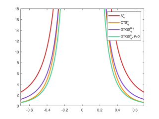
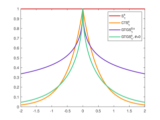
Figure 1: Left panel: $S$, CTS${}^{s}_{\gamma}$, GTGS${}^{s}_{\gamma}$, and GTGS${}^{0,s}_{\gamma}$ Lévy densities. Right panel: corresponding tempering functions. The parameters are $\gamma=1.6,\alpha=0.5,\lambda=\theta=\delta=1$.

Symbol	Description	Dimension
BG$({\bm{\lambda}},{\bm{\delta}})$	bilateral gamma	1
BL$({\bm{\alpha}},{\bm{\lambda}},{\bm{\delta}})$	bilateral Linnik	1
CTS${}_{{\bm{\gamma}}}({\bm{\theta}},{\bm{\delta}};\mu)$	classical tempered-stable	1
G$(\lambda,\delta)$	gamma	1
GTGS${}_{{\bm{\gamma}}}({\bm{\alpha}},{\bm{\lambda}},{\bm{\theta}},{\bm{\delta}};\mu)$	generalized tempered geometric stable	1
GTGS${}_{\gamma}(\sigma,\alpha,\lambda,\theta;\mu)$	GTGS, spherical parametrization	$d$
GTGS${}_{\gamma}(r_{\gamma}(x;{\bm{\alpha}},{\bm{\lambda}},{\bm{\theta}},{\bm{\delta}});\mu)$	GTGS, Rosińsky parametrization	1
GTGS${}_{\bm{\gamma}}^{0}({\bm{\alpha}},{\bm{\lambda}},{\bm{\delta}};\mu)$	purely Mittag-Leffler tempered GTGS	1
ML$(\alpha,\lambda)$	Mittag-Leffler	1
PL$(\alpha,\lambda,\delta)$	positive Linnik	1
S${}_{\alpha}(\lambda,\beta;\mu)$	$\alpha$-stable, classical parametrization	1
S${}_{{\bm{\alpha}}}({\bm{\delta}};\mu)$	$\alpha$-stable, Lévy parametrization	1
S${}_{\alpha}(\sigma,\mu)$	$\alpha$-stable, spherical parametrization	$d$
TGS${}_{\bm{\alpha}}({\bm{\lambda}},{\bm{\theta}},{\bm{\delta}};\mu)$	tempered geometric stable	1
TGS$(\sigma,\alpha,\lambda,\theta;\mu)$	TGS, spherical parametrization	$d$
TGS${}^{0}_{\bm{\alpha}}({\bm{\lambda}},{\bm{\delta}};\mu)$	purely Mittag-Leffler tempered TGS	1
TPL$(\alpha,\lambda,\theta,\delta)$	tempered positive Linnik	1
TS${}_{\gamma}(Q;\mu)$	Rosińsky tempered stable, spectral parametrization	$d$
TS${}_{\gamma}(R;\mu)$	Rosińsky tempered stable, Rosińsky parametrization	$d$

Table 1: Distribution list. When appearing, the superscripts $s,+,-$ stand respectively for the symmetric, spectrally positive and spectrally negative version of the corresponding distribution.

Declarations

This research did not receive any specific grant from funding agencies in the public, commercial, or not-for-profit sectors. The author declares no competing interests.

References

- (1) Barabesi, L., Cerasa, A., Perrotta, D., and Cerioli, A. (2016a). Modeling international trade data with the Tweedie distribution for anti-fraud and policy support. European Journal of Operational Research, 248:1031–1043.
- (2) Barabesi, L., Cerasa, A., Perrotta, D., and Cerioli, A. (2016b). A new family of tempered distributions. Electronic Journal of Statistics, 10:3871–3893.
- Boyarchenko and Levendorskiĭ, (2000) Boyarchenko, S. I. and Levendorskiĭ, S. Z. (2000). Option pricing for truncated Lévy processes. International Journal of Theoretical and Applied Finance, 3:549–552.
- Braaksma, (1963) Braaksma, B. L. J. (1963). Asymptotic expansions and analytic continuations for a class of Barnes-integrals. Compositio Mathematica, 15:239–341.
- Carr et al., (2002) Carr, P., Geman, H., Madan, D. B., and Yor, M. (2002). The fine structure of asset returns: an empirical investigation. Journal of Business, 75:305–332.
- Chechkin et al., (2008) Chechkin, A. V., Metzler, R., Klafter, J., and Gonchar, V. Y. (2008). Introduction to the theory of Lévy flights. Anomalous transport: Foundations and applications, pages 129–162.
- Christoph and Schreiber, (2001) Christoph, G. and Schreiber, K. (2001). Positive Linnik and discrete Linnik distributions. In Balakrishnan, N., Ibragimov, I. V., and Nevzorov, V. B., editors, Asymptotic Methods in Probability and Statistics with Applications, pages 3–17. Birkhäuser, Boston.
- Cohen and Rosiński, (2007) Cohen, S. and Rosiński, J. (2007). Gaussian approximation of multivariate Lévy processes with applications to simulation of tempered stable processes. Bernoulli, 13:195–210.
- Cont and Tankov, (2003) Cont, R. and Tankov, P. (2003). Financial Modelling with Jump Processes. Chapman and Hall/CRC Press.
- De Oliveira et al., (2011) De Oliveira, E. C., Mainardi, F., and Vaz, J. (2011). Models based on Mittag-Leffler functions for anomalous relaxation in dielectrics. The European Physical Journal Special Topics, 193:161–171.
- Dotsenko, (1991) Dotsenko, M. R. (1991). On some applications of Wright’s hypergeometric function. Dokladi Na Bolgarskata Akademiya Na Naukite, 44:13–16.
- Ferreira et al., (2017) Ferreira, E. M., Kohara, A. K., and Sesma, J. (2017). New properties of the Lerch’s transcendent. Journal of Number Theory, 172:21–31.
- Garra and Garrappa, (2018) Garra, R. and Garrappa, R. (2018). The Prabhakar or three parameter Mittag–Leffler function: Theory and application. Communications in Nonlinear Science and Numerical Simulation, 56:314–329.
- Gopikrishnan et al., (1998) Gopikrishnan, P., Meyer, M., Amaral, L. N., and Stanley, H. E. (1998). Inverse cubic law for the distribution of stock price variations. The European Physical Journal B-Condensed Matter and Complex Systems, 3:139–140.
- Gopikrishnan et al., (1999) Gopikrishnan, P., Plerou, V., Amaral, L. A. N., Meyer, M., and Stanley, H. E. (1999). Scaling of the distribution of fluctuations of financial market indices. Physical Review E, 60:5305.
- Gorenflo et al., (2020) Gorenflo, R., Kilbas, A. A., Mainardi, F., and Rogosin, S. (2020). Mittag-Leffler Functions, Related Topics and Applications. Second Edition. Springer, Berlin.
- Górska et al., (2021) Górska, K., Horzela, A., Lattanzi, A., and Pogány, T. K. (2021). On complete monotonicity of three parameter Mittag-Leffler function. Applicable Analysis and Discrete Mathematics, 15:118–128.
- Grabchak, (2016) Grabchak, M. (2016). Tempered Stable Distributions: Stochastic Models for Multiscale Processes. Springer, Cham.
- Guillera and Jonathan, (2008) Guillera, J. and Jonathan, S. (2008). Double integrals and infinite products for some classical constants via analytic continuation of Lerch’s trascendent. The Ramanujan Journal, 16:247–270.
- Haubold et al., (2011) Haubold, H. J., Mathai, A. M., and Saxena, R. K. (2011). Mittag-Leffler functions and their applications. Journal of Applied Mathematics. Article ID 298628.
- James, (2006) James, L. F. (2006). Gamma tilting calculus for GGC and Dirichlet means with applications to Linnik processes and occupation time laws for randomly skewed Bessel processes and bridges. ArXiv preprint. arXiv: 0610218.
- Kallenberg, (2002) Kallenberg, O. (2002). Foundations of Modern Probability. Springer-Verlag.
- Karp and Prilepkina, (2020) Karp, D. and Prilepkina, E. G. (2020). The Fox-Wright function near the singularity and the branch cut. Journal of Mathematical Analysis and Applications, 484:123664.
- Kilbas et al., (2003) Kilbas, A. A., Saxena, R., Saigo, M., and Trujillo, J. J. (2003). Generalized Wright function as the H-function. Analytic Methods of Analysis and Differential Equations, AMADE, pages 117–134.
- (25) Kim, Y. S., Rachev, S. T., Bianchi, M. L., and Fabozzi, F. J. (2009a). A new tempered stable distribution and its application to finance. In Risk Assessment, pages 77–109. Springer.
- (26) Kim, Y. S., Rachev, S. T., Chung, D. M., and Bianchi, M. L. (2009b). The modified tempered stable distribution, GARCH-models and option pricing. Probability and Mathematical Statistics, 29:91–117.
- Klebanov et al., (1985) Klebanov, L. B., Maniya, G. M., and Melamed, I. A. (1985). A problem of Zolotarev and analogs of infinitely divisible and stable distributions in a scheme for summing a random number of random variables. Theory of Probability and its Applications, 29:791–794.
- Koponen, (1995) Koponen, I. (1995). Analytic approach to the problem of convergence of truncated Lévy flights towards the Gaussian stochastic process. Physical Review E, 52:1197–1199.
- Kotz et al., (2001) Kotz, S., Kozubowski, T. J., and Podgórski, K. (2001). Asymmetric multivariate Laplace distribution. In The Laplace Distribution and Generalizations, pages 239–272. Springer.
- Kozubowski and Podgórski, (2001) Kozubowski, T. J. and Podgórski, K. (2001). Asymmetric Laplace laws and modeling financial data. Mathematical and Computer Modelling, 34:1003–1021.
- Kozubowski et al., (1999) Kozubowski, T. J., Podgórski, K., and Samorodnitsky, G. (1999). Tails of Lévy measure of geometric stable random variables. Extremes, 1:367–378.
- Kozubowski and Rachev, (1999) Kozubowski, T. J. and Rachev, S. T. (1999). Univariate geometric stable laws. Journal of Computational Analysis and Applications, 1:177–217.
- Küchler and Tappe, (2008) Küchler, U. and Tappe, S. (2008). Bilateral gamma distributions and processes in financial mathematics. Stochastic Processes and their Applications, 118:261–283.
- Küchler and Tappe, (2013) Küchler, U. and Tappe, S. (2013). Tempered stable distributions and processes. Stochastic processes and their applications, 123:4256–4293.
- Kumar et al., (2019) Kumar, A., Upadhye, N. S., Wylomanska, A., and Gajda, J. (2019). Tempered Mittag-Leffler Lévy processes. Communications in Statistics – Theory and Methods, 48:396–411.
- Lin, (1998) Lin, G. D. (1998). A note on the Linnik distributions. Journal of Mathematical Analysis and Applications, 217:701–706.
- Linnik, (1963) Linnik, Y. V. (1963). Linear forms and statistical criteria, I, II. Selected Translations in Mathematical Statistics and Probability, 3:1–90.
- Longin, (1996) Longin, F. M. (1996). The asymptotic distribution of extreme stock market returns. Journal of Business, pages 383–408.
- Lukacs et al., (1952) Lukacs, E., Szász, O., et al. (1952). On analytic characteristic functions. Pacific J. Math, 2:615–625.
- Lux, (1996) Lux, T. (1996). The stable Paretian hypothesis and the frequency of large returns: an examination of major German stocks. Applied Financial Economics, 6:463–475.
- Mantegna and Stanley, (1994) Mantegna, R. N. and Stanley, H. E. (1994). Stochastic process with ultraslow convergence to a Gaussian: the truncated Lévy flight. Physical Review Letters, 73:2946–2949.
- Meerschaert et al., (2011) Meerschaert, M., Nane, E., and Vellaisamy, P. (2011). The fractional Poisson process and the inverse stable subordinator. Electronic Journal of Probability, 16:1600–1620.
- Mittnik and Rachev, (1991) Mittnik, S. and Rachev, S. T. (1991). Alternative multivariate stable distributions and their applications to financial modeling. In Cambanis, S., Samorodnitsky, G., and Taqqu, M. S., editors, Stable Processes and Related Topics, pages 107–119. Birkäuser, Boston.
- Pakes, (1998) Pakes, A. G. (1998). Mixture representations for symmetric generalized Linnik laws. Statistics and Probability Letters, 37:213–221.
- Pillai, (1990) Pillai, R. N. (1990). On Mittag-Leffler functions and related distributions. Annals of the Institute of Statistical Mathematics, 42:157–161.
- Plerou et al., (1999) Plerou, V., Gopikrishnan, P., Amaral, L. A. N., Meyer, M., and Stanley, H. E. (1999). Scaling of the distribution of price fluctuations of individual companies. Physical Review E, 60:6519.
- Pollard, (1948) Pollard, H. (1948). The completely monotonic character of the mittag-leffler function . Bulletin of the American Mathematical Society, 54:1115–1116.
- Prabhakar, (1971) Prabhakar, T. R. (1971). A singular integral equation with a generalized Mittag Leffler function in the kernel. Yokohama Mathematical Journal, 19:7–15.
- Rosiński, (2007) Rosiński, J. (2007). Tempering stable processes. Stochastic processes and their applications, 117:677–707.
- Rosiński and Sinclair, (2010) Rosiński, J. and Sinclair, J. L. (2010). Generalized tempered stable processes. Stability in Probability, 90:153–170.
- Sandhya and Pillai, (1999) Sandhya, E. and Pillai, R. N. (1999). On geometric infinite divisibility. Journal of the Kerala Statistical Association, 10:1–7. ArXiv preprint. arXiv:1409.4022.
- Sato, (1999) Sato, K. (1999). Lévy Processes and Infinitely Divisible Distributions. Cambridge University Press.
- Sato and Yamazato, (1978) Sato, K. and Yamazato, M. (1978). On distribution functions of class L. Zeitschrift für Wahrscheinlichkeitstheorie und verwandte Gebiete, 43:273–308.
- Schilling et al., (2012) Schilling, R. L., Song, R., and Vondraček, Z. (2012). Bernstein Functions: Theory and Applications. Second Edition. De Gruyter, Berlin.
- Šikić et al., (2006) Šikić, H., Song, R., and Vondraček, Z. (2006). Potential theory of geometric stable processes. Probability Theory and Related Fields, 135:547–575.
- Sokolov et al., (2004) Sokolov, I. M., Chechkin, A. V., and Klafter, J. (2004). Fractional diffusion equation for a power-law-truncated Lévy process. Physica A: Statistical Mechanics and its Applications, 336(3-4):245–251.
- Stanley, (2003) Stanley, H. E. (2003). Statistical physics and economic fluctuations: do outliers exist? Physica A: Statistical Mechanics and its Applications, 318:279–292.
- Steutel and Van Harn, (2004) Steutel, F. W. and Van Harn, K. (2004). Infinite Divisibility of Probability Distributions on the Real Line. Dekker, New York.
- Terdik and Woyczynski, (2006) Terdik, G. and Woyczynski, W. (2006). Rosiński measures for tempered stable and related Ornstein-Uhlenbeck processes. Probability and Mathematical Statistics, 26:213.
- Torricelli et al., (2022) Torricelli, L., Barabesi, L., and A., C. (2022). Tempered positive Linnik processes and their representations. Electronic Journal of Statistics, 16:6313–6347.
- Virchenko et al., (2001) Virchenko, N., Kalla, S., and Al-Zamel, A. (2001). Some results on a generalized hypergeometric function. Integral Transforms and Special Functions, 12:89–100.
- Watanabe, (2008) Watanabe, T. (2008). Convolution equivalence and distributions of random sums. Probability Theory and Related Fields, 142:367–397.
- Watanabe and Yamamuro, (2010) Watanabe, T. and Yamamuro, K. (2010). Ratio of the tail of an infinitely divisible distribution on the line to that of its Lévy measure. Electronic Journal of Probability, 15:44–74.
- Wolfe, (1971) Wolfe, S. J. (1971). On the continuity properties of L functions. The Annals of Mathematical Statistics, pages 2064–2073.
- Wright, (1935) Wright, E. M. (1935). The asymptotic expansion of the generalized hypergeometric function. Journal of the London Mathematical Society, 10:286–293.
- Yamazato, (1978) Yamazato, M. (1978). Unimodality of infinitely divisible distribution functions of class L. The Annals of Probability, pages 523–531.
- Zolotarev, (1963) Zolotarev, V. M. (1963). Structure of the infinitely divisible laws of L-class. Lithuanian Mathematical Journal, 3:123–140.