All Points Matter: Entropy-Regularized Distribution Alignment for Weakly-supervised 3D Segmentation

Abstract

Pseudo-labels are widely employed in weakly supervised 3D segmentation tasks where only sparse ground-truth labels are available for learning. Existing methods often rely on empirical label selection strategies, such as confidence thresholding, to generate beneficial pseudo-labels for model training. This approach may, however, hinder the comprehensive exploitation of unlabeled data points. We hypothesize that this selective usage arises from the noise in pseudo-labels generated on unlabeled data. The noise in pseudo-labels may result in significant discrepancies between pseudo-labels and model predictions, thus confusing and affecting the model training greatly. To address this issue, we propose a novel learning strategy to regularize the generated pseudo-labels and effectively narrow the gaps between pseudo-labels and model predictions. More specifically, our method introduces an Entropy Regularization loss and a Distribution Alignment loss for weakly supervised learning in 3D segmentation tasks, resulting in an ERDA learning strategy. Interestingly, by using KL distance to formulate the distribution alignment loss, it reduces to a deceptively simple cross-entropy-based loss which optimizes both the pseudo-label generation network and the 3D segmentation network simultaneously. Despite the simplicity, our method promisingly improves the performance. We validate the effectiveness through extensive experiments on various baselines and large-scale datasets. Results show that ERDA effectively enables the effective usage of all unlabeled data points for learning and achieves state-of-the-art performance under different settings. Remarkably, our method can outperform fully-supervised baselines using only 1% of true annotations. Code and model will be made publicly available at https://github.com/LiyaoTang/ERDA.

1 Introduction

Point cloud semantic segmentation is a crucial task for 3D scene understanding and has various applications ptsurvey ; ptSreview , such as autonomous driving, unmanned aerial vehicles, and augmented reality. Current state-of-the-art approaches heavily rely on large-scale and densely annotated 3D datasets, which are costly to obtain weak_survey ; sensat . To avoid demanding exhaustive annotation, weakly-supervised point cloud segmentation has emerged as a promising alternative. It aims to leverage a small set of annotated points while leaving the majority of points unlabeled in a large point cloud dataset for learning. Although current weakly supervised methods can offer a practical and cost-effective way to perform point cloud segmentation, their performance is still sub-optimal compared to fully-supervised approaches.

During the exploration of weak supervision weak_10few , a significant challenge is the insufficient training signals provided by the highly sparse labels. To tackle this issue, pseudo-labeling methods weak_10few ; weak_color ; weak_sqn have been proposed, which leverage predictions on unlabeled points as labels to facilitate the learning of the segmentation network. Despite some promising results, these pseudo-label methods have been outperformed by some recent methods based on consistency regularization weak_hybrid ; weak_mil . We tend to attribute this to the use of label selection on pseudo-labels, such as confidence thresholding, which could lead to unlabeled points being wasted and under-explored. We hypothesize that the need for label selection arises from the low-confidence pseudo-labels assigned to unlabeled points, which are known for their noises weak_survey and potential unintended bias calib_pseudo ; weak_2d_dycls . These less reliable and noisy pseudo-labels could contribute to discrepancies between the pseudo-labels and the model predictions, which might confuse and impede the learning process to a great extent.

By addressing the above problem for label selection in weakly supervised 3D segmentation, we propose a novel learning-based approach in this study. Our method aims to leverage the information from all unlabeled points by mitigating the negative effects of the noisy pseudo-labels and the distributional discrepancy.

Specifically, we introduce two learning objectives for the pseudo-label generation process. Firstly, we introduce an entropy regularization (ER) objective to reduce the noise and uncertainty in the pseudo-labels. This regularization promotes more informative, reliable, and confident pseudo-labels, which helps alleviate the limitations of noisy and uncertain pseudo-labels. Secondly, we propose a distribution alignment (DA) loss that minimizes statistical distances between pseudo-labels and model predictions. This ensures that the distribution of generated pseudo-labels remains close to the distribution of model predictions when regularizing their entropy.

In particular, we discover that formulating the distribution alignment loss using KL distance enables a simplification of our method into a cross-entropy-style learning objective that optimizes both the pseudo-label generator and the 3D segmentation network simultaneously. This makes our method straightforward to implement and apply. By integrating the entropy regularization and distribution alignment, we achieve the ERDA learning strategy, as shown in Fig. 1.

Empirically, we comprehensively experiment with three baselines and different weak supervision settings, including 0.02% (1-point, or 1pt), 1%, and 10%. Despite its concise design, our ERDA outperforms existing weakly-supervised methods on large-scale point cloud datasets such as S3DIS s3dis , ScanNet scannet , and SensatUrban sensat . Notably, our ERDA can surpass the fully-supervised baselines using only 1% labels, demonstrating its significant effectiveness in leveraging pseudo-labels. Furthermore, we validate the scalability of our method by successfully generalizing it to more other settings, which illustrates the benefits of utilizing dense pseudo-label supervision with ERDA.

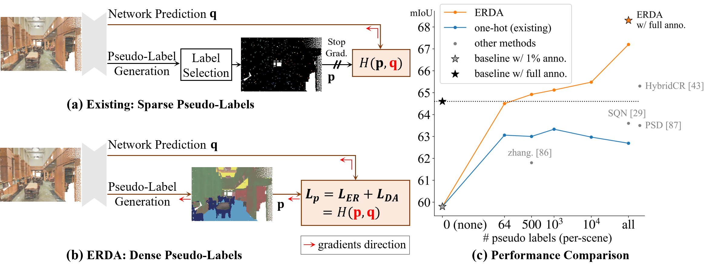
Figure 1: While existing pseudo-labels (a) are limited in the exploitation of unlabeled points, ERDA (b) simultaneously optimizes the pseudo-labels $\mathbf{p}$ and predictions $\mathbf{q}$ taking the same and simple form of cross-entropy. By reducing the noise via entropy regularization and bridging their distributional discrepancies, ERDA produces informative pseudo-labels that neglect the need for label selection. As in (c), it thus enables the model to consistently benefit from more pseudo-labels, surpasses other methods and its fully-supervised baseline, and can be extended to advance the fully-supervised performance.

2 Related Work

Point cloud segmentation.

Point cloud semantic segmentation aims to assign semantic labels to 3D points. The cutting-edge methods are deep-learning-based and can be classified into projection-based and point-based approaches. Projection-based methods project 3D points to grid-like structures, such as 2D image seg_mv_SqueezeSegV3 ; seg_mv_RangeNet ; vmvf ; others_roaddet ; seg_mv_snapNet ; seg_mv_proj or 3D voxels Minkowski ; ocnn ; seg_vx_SEGCloud ; occuseg ; seg_vx_SSCN ; cls_vx_sparseConvSubmanifold ; seg_vx_voxsegnet . Alternatively, point-based methods directly operate on 3D points pointnet ; pointnet++ . Recent efforts have focused on novel modules and backbones to enhance point features, such as 3D convolution fkaconv ; pointcnn ; pointconv ; kpconv ; closerlook ; pointnext , attentions randlanet ; pct ; pttransformer ; pttransformerv2 ; stratified ; cdformer , graph-based methods dgcnn ; spg , and other modules such as sampling sample ; PointASNL ; pat ; others_sasa and post-processing bound_3d_cga ; bound_3d_jse ; bound_cbl . Although these methods have made significant progress, they rely on large-scale datasets with point-wise annotation and struggle with few labels weak_10few . To address the demanding requirement of point-wise annotation, our work explores weakly-supervised learning for 3D point cloud segmentation.

Weakly-supervised point cloud segmentation.

Compared to weakly-supervised 2D image segmentation weak_2d_cam ; weak_2d_scrible ; weak_2d_unreliable ; weak_2d_affinity ; weak_2d_fixmatch , weakly-supervised 3D point cloud segmentation is less explored. In general, weakly-supervised 3D segmentation task focus on highly sparse labels: only a few scattered points are annotated in large point cloud scenes. Xu and Lee weak_10few first propose to use 10x fewer labels to achieve performance on par with a fully-supervised point cloud segmentation model. Later studies have explored more advanced ways to exploit different forms of weak supervision weak_multipath ; weak_box2mask ; weak_joint2d3d and human annotations weak_otoc ; weak_scribble . Recent methods tend to introduce perturbed self-distillation weak_psd , consistency regularization weak_10few ; weak_4d ; weak_rac ; weak_dat ; weak_plconst , and leverage self-supervised learning weak_4d ; weak_cl ; weak_hybrid ; weak_mil based on contrastive learning moco ; simclr . Pseudo-labels are another approach to leverage unlabeled data, with methods such as pre-training networks on colorization tasks weak_color , using iterative training weak_sqn , employing separate networks to iterate between learning pseudo-labels and training 3D segmentation networks weak_otoc , or using super-point graph spg with graph attentional module to propagate the limited labels over super-points weak_sspc . However, these existing methods often require expensive training due to hand-crafted 3D data augmentations weak_psd ; weak_mil ; weak_rac ; weak_dat , iterative training weak_otoc ; weak_sqn , or additional modules weak_mil ; weak_sqn , complicating the adaptation of backbone models from fully-supervised to weakly-supervised learning. In contrast, our work aims to achieve effective weakly supervised learning for the 3D segmentation task with straightforward motivations and simple implementation.

Pseudo-label refinement.

Pseudo-labeling pseudo_simple , a versatile method for entropy minimization weak_2d_entropy , has been extensively studied in various tasks, including semi-supervised 2D classification 2d_noisystudent ; calib_pseudo , segmentation weak_2d_fixmatch ; weak_2d_unimatch , and domain adaptation pseudo_da_rectify ; pseudo_da_uncertain . To generate high-quality supervision, various label selection strategies have been proposed based on learning status weak_2d_freematch ; weak_2d_flexmatch ; pseudo_2d_dmt , label uncertainty calib_pseudo ; pseudo_da_rectify ; pseudo_da_uncertain ; weak_2d_PMT , class balancing weak_2d_dycls , and data augmentations weak_2d_fixmatch ; weak_2d_unimatch ; weak_2d_dycls . Our method is most closely related to the works addressing bias in supervision, where mutual learning pseudo_2d_dmt ; pseudo_2d_rep ; weak_2d_rml and distribution alignment weak_2d_dycls ; weak_2d_redistr ; weak_2d_ELN have been discussed. However, these works typically focus on class imbalance weak_2d_dycls ; weak_2d_redistr and rely on iterative training pseudo_2d_rep ; pseudo_2d_dmt ; weak_2d_rml ; weak_2d_ELN , label selection pseudo_2d_dmt ; weak_2d_redistr , and strong data augmentations weak_2d_dycls ; weak_2d_redistr , which might not be directly applicable to 3D point clouds. For instance, common image augmentations weak_2d_fixmatch like cropping and resizing may translate to point cloud upsampling ptsurvey_up , which remains an open question in the related research area. Rather than introducing complicated mechanisms, we argue that proper regularization on pseudo-labels and its alignment with model prediction can provide significant benefits using a very concise learning approach designed for the weakly supervised 3D point cloud segmentation task.

Besides, it is shown that the data augmentations and repeated training in mutual learning pseudo_2d_rep ; noise_2d_pencil are important to avoid the feature collapse, i.e., the resulting pseudo-labels being uniform or the same as model predictions. We suspect the cause may originate from the entropy term in their use of raw statistical distance by empirical results, which potentially matches the pseudo-labels to noisy and confusing model prediction, as would be discussed in Sec. 3.2. Moreover, in self-supervised learning based on clustering swav and distillation dino , it has also been shown that it would lead to feature collapse if matching to a cluster assignment or teacher output of a close-uniform distribution with high entropy, which agrees with the intuition in our ER term.

3 Methodology

3.1 Formulation of ERDA

As previously mentioned, we propose the ERDA approach to alleviate noise in the generated pseudo-labels and reduce the distribution gaps between them and the segmentation network predictions. In general, our ERDA introduces two loss functions, including the entropy regularization loss and the distribution alignment loss for the learning on pseudo-labels. We denote the two loss functions as $L_{ER}$ and $L_{DA}$, respectively. Then, we have the overall loss of ERDA as follows:

$$L_{p}=\lambda L_{ER}+L_{DA},$$ (1)

where the $\lambda>0$ modulates the entropy regularization which is similar to the studies  pseudo_simple ; weak_2d_entropy .

Before detailing the formulation of $L_{ER}$ and $L_{DA}$, we first introduce the notation. While the losses are calculated over all unlabeled points, we focus on one single unlabeled point for ease of discussion. We denote the pseudo-label assigned to this unlabeled point as $\mathbf{p}$ and the corresponding segmentation network prediction as $\mathbf{q}$. Each $\mathbf{p}$ and $\mathbf{q}$ is a 1D vector representing the probability over classes.

Entropy Regularization loss.

We hypothesize that the quality of pseudo-labels can be hindered by noise, which in turn affects model learning. Specifically, we consider that the pseudo-label could be more susceptible to containing noise when it fails to provide a confident pseudo-labeling result, which leads to the presence of a high-entropy distribution in $\mathbf{p}$.

To mitigate this, for the $\mathbf{p}$, we propose to reduce its noise level by minimizing its Shannon entropy, which also encourages a more informative labeling result shannon . Therefore, we have:

$$L_{ER}=H(\mathbf{p}),$$ (2)

where $H(\mathbf{p})=\sum_{i}-p_{i}\log p_{i}$ and $i$ iterates over the vector. By minimizing the entropy of the pseudo-label as defined above, we promote more confident labeling results to help resist noise in the labeling process.

Distribution Alignment loss.

In addition to the noise in pseudo-labels, we propose that significant discrepancies between the pseudo-labels and the segmentation network predictions could also confuse the learning process and lead to unreliable segmentation results. In general, the discrepancies can stem from multiple sources, including the noise-induced unreliability of pseudo-labels, differences between labeled and unlabeled data weak_2d_dycls , and variations in pseudo-labeling methods and segmentation methods weak_2d_rml ; pseudo_2d_dmt . Although entropy regularization could mitigate the impact of noise in pseudo-labels, significant discrepancies may still persist between the pseudo-labels and the predictions of the segmentation network. To mitigate this issue, we propose that the pseudo-labels and network can be jointly optimized to narrow such discrepancies, making generated pseudo-labels not diverge too far from the segmentation predictions. Therefore, we introduce the distribution alignment loss.

To properly define the distribution alignment loss ($L_{DA}$), we measure the KL divergence between the pseudo-labels ($\mathbf{p}$) and the segmentation network predictions ($\mathbf{q}$) and aim to minimize this divergence. Specifically, we define the distribution alignment loss as follows:

$$L_{DA}=KL(\mathbf{p}||\mathbf{q}),$$ (3)

where $KL(\mathbf{p}||\mathbf{q})$ refers to the KL divergence. Using the above formulation has several benefits. For example, the KL divergence can simplify the overall loss $L_{p}$ into a deceptively simple form that demonstrates desirable properties and also performs better than other distance measurements. More details will be presented in the following sections.

Simplified ERDA.

With the $L_{ER}$ and $L_{DA}$ formulated as above, given that $KL(\mathbf{p}||\mathbf{q})=H(\mathbf{p},\mathbf{q})-H(\mathbf{p})$ where $H(\mathbf{p},\mathbf{q})$ is the cross entropy between $\mathbf{p}$ and $\mathbf{q}$, we can have a simplified ERDA formulation as:

$$L_{p}=H(\mathbf{p},\mathbf{q})+(\lambda-1)H(\mathbf{p}).$$ (4)

In particular, when $\lambda=1$, we obtain the final ERDA loss:

$$L_{p}=H(\mathbf{p},\mathbf{q})=\sum_{i}-p_{i}\log q_{i}$$ (5)

The above simplified ERDA loss describes that the entropy regularization loss and distribution alignment loss can be represented by a single cross-entropy-based loss that optimizes both $\mathbf{p}$ and $\mathbf{q}$.

We would like to emphasize that Eq. 5 is distinct from the conventional cross-entropy loss. The conventional cross-entropy loss utilizes a fixed label and only optimizes the term within the logarithm function, whereas the proposed loss in Eq. 5 optimizes both $\mathbf{p}$ and $\mathbf{q}$ simultaneously.

3.2 Delving into the Benefits of ERDA

To formulate the distribution alignment loss, different functions can be employed to measure the differences between $\mathbf{p}$ and $\mathbf{q}$. In addition to the KL divergence, there are other distance measurements like mean squared error (MSE) or Jensen-Shannon (JS) divergence for replacement. Although many mutual learning methods pseudo_2d_dmt ; weak_2d_rml ; weak_2d_ELN ; noise_2d_pencil have proven the effectiveness of KL divergence, a detailed comparison of KL divergence against other measurements is currently lacking in the literature. In this section, under the proposed ERDA learning framework, we show by comparison that $KL(\mathbf{p}||\mathbf{q})$ is a better choice and ER is necessary for weakly-supervised 3D segmentation.

To examine the characteristics of different distance measurements, including $KL(\mathbf{p}||\mathbf{q})$, $KL(\mathbf{q}||\mathbf{p})$, $JS(\mathbf{p}||\mathbf{q})$, and $MSE(\mathbf{p}||\mathbf{q})$, we investigate the form of our ERDA loss $L_{p}$ and its impact on the learning for pseudo-label generation network given two situations during training.

More formally, we shall assume a total of $K$ classes and define that a pseudo-label $\mathbf{p}=[p_{1},...,p_{K}]$ is based on the confidence scores $\mathbf{s}=[s_{1},...,s_{K}]$, and that $\mathbf{p}=\text{softmax}(\mathbf{s})$. Similarly, we have a segmentation network prediction $\mathbf{q}=[q_{1},...,q_{K}]$ for the same point. We re-write the ERDA loss $L_{p}$ in various forms and investigate the learning from the perspective of gradient update, as in Tab. 1.

Situation 1: Gradient update given confident pseudo-label $\mathbf{p}$.

We first specifically study the case when $\mathbf{p}$ is very certain and confident, i.e., $\mathbf{p}$ approaching a one-hot vector. As in Tab. 1, most distances yield the desired zero gradients, which thus retain the information of a confident and reliable $\mathbf{p}$. In this situation, however, the $KL(\mathbf{q}||\mathbf{p})$, rather than $KL(\mathbf{p}||\mathbf{q})$ in our method, produces non-zero gradients that would actually increase the noise among pseudo-labels during its learning, which is not favorable according to our motivation.

Situation 2: Gradient update given confusing prediction $\mathbf{q}$.

In addition, we are also interested in how different choices of distance and $\lambda$ would impact the learning on pseudo-label if the segmentation model produces confusing outputs, i.e., $\mathbf{q}$ tends to be uniform. In line with the motivation of ERDA learning, we aim to regularize the pseudo-labels to mitigate potential noise and bias, while discouraging uncertain labels with little information. However, as in Tab. 1, most implementations yield non-zero gradient updates to the pseudo-label generation network. This update would make $\mathbf{p}$ closer to the confused $\mathbf{q}$, thus increasing the noise and degrading the training performance. Conversely, only $KL(\mathbf{p}||\mathbf{q})$ can produce a zero gradient when integrated with the entropy regularization with $\lambda=1$. That is, only ERDA in Eq. 5 would not update the pseudo-label generation network when $\mathbf{q}$ is not reliable, which avoids confusing the $\mathbf{p}$. Furthermore, when $\mathbf{q}$ is less noisy but still close to a uniform vector, it is indicated that there is a large close-zero plateau on the gradient surface of ERDA, which benefits the learning on $\mathbf{p}$ by resisting the influence of noise in $\mathbf{q}$.

In addition to the above cases, the gradients of ERDA in Eq. 5 could be generally regarded as being aware of the noise level and the confidence of both pseudo-label $\mathbf{p}$ and the corresponding prediction $\mathbf{q}$. Especially, ERDA produces larger gradient updates on noisy pseudo-labels, while smaller updates on confident and reliable pseudo-labels or given noisy segmentation prediction. Therefore, our formulation demonstrates its superiority in fulfilling our motivation of simultaneous noise reduction and distribution alignment, where both $L_{ER}$ and KL-based $L_{DA}$ are necessary. We provide more empirical studies in ablation (Sec. 4.3) and detailed analysis in the supplementary.

$\displaystyle L_{DA}$	$\displaystyle KL(\mathbf{p}||\mathbf{q})$	$\displaystyle KL(\mathbf{q}||\mathbf{p})$	$\displaystyle JS(\mathbf{p},\mathbf{q})$	$\displaystyle MSE(\mathbf{p},\mathbf{q})$
$\displaystyle L_{p}$	$\displaystyle H(\mathbf{p},\mathbf{q})-(1-\lambda)H(\mathbf{p})$	$\displaystyle H(\mathbf{q},\mathbf{p})-H(\mathbf{q})+\lambda H(\mathbf{p})$	$\displaystyle H(\frac{\mathbf{p}+\mathbf{q}}{2})-(\frac{1}{2}-\lambda)H(\mathbf{p})-\frac{1}{2}H(\mathbf{q})$	$\displaystyle\frac{1}{2}\sum_{i}(p_{i}-q_{i})^{2}+\lambda H(\mathbf{p})$
S1	$\displaystyle 0$	$\displaystyle q_{i}-\mathbb{1}_{k=i}$	$\displaystyle 0$	$\displaystyle 0$
S2	$\displaystyle(\lambda-1)p_{i}\sum_{j}p_{j}\log\frac{p_{i}}{p_{j}}$	$\displaystyle\frac{1}{K}-p_{i}+\lambda p_{i}\sum_{j}p_{j}\log\frac{p_{i}}{p_{j}}$	$\displaystyle p_{i}\sum_{j\neq i}p_{j}(\frac{1}{2}\log\frac{Kp_{i}+1}{Kp_{j}+1}+(\lambda-\frac{1}{2})\log\frac{p_{i}}{p_{j}})$	$\displaystyle-p_{i}^{2}+p_{i}\sum_{j}p_{j}^{2}+\lambda p_{i}\sum_{j}p_{j}\log\frac{p_{i}}{p_{j}}$

Table 1: The formulation of $L_{p}$ using different functions to formulate $L_{DA}$. We study the gradient update on $s_{i}$, i.e., $-\frac{\partial L_{p}}{\partial s_{i}}$ under different situations. S1: update given confident pseudo-label, $\mathbf{p}$ being one-hot with $\exists p_{k}\in\mathbf{p},p_{k}\rightarrow 1$. S2: update given confusing prediction, $\mathbf{q}$ being uniform with $q_{1}=...=q_{K}=\frac{1}{K}$. More analysis as well as visualization can be found in the Sec. 3.2 and the supplementary Appendix C.

3.3 Implementation Details on Pseudo-Labels

In our study, we use a prototypical pseudo-label generation process due to its popularity as well as simplicity weak_color . Specifically, prototypes proto denote the class centroids in the feature space, which are calculated based on labeled data, and pseudo-labels are estimated based on the feature distances between unlabeled points and class centroids.

As shown in Fig. 2, we use a momentum-based prototypical pseudo-label generation process due to its popularity as well as simplicity weak_color ; weak_10few ; pseudo_gearbox . Specifically, prototypes proto denote the class centroids in the feature space, which are calculated based on labeled data, and pseudo-labels are estimated based on the feature distances between unlabeled points and class centroids. To avoid expensive computational costs and compromised representations for each semantic class weak_color ; weak_mil ; weak_hybrid , momentum update is utilized as an approximation for global class centroids.

Based on the momentum-updated prototypes, we attach an MLP-based projection network to help generate pseudo-labels and learn with our method. Aligned with our motivation, we do not introduce thresholding-based label selection or one-hot conversion pseudo_simple ; weak_color to process generated pseudo-labels. More details are in the supplementary.

More formally, we take as input a point cloud $\mathcal{X}$, where the labeled points are $\mathcal{X}^{l}$ and the unlabeled points are $\mathcal{X}^{u}$. For a labeled point $\mathbf{x}\in\mathcal{X}^{l}$, we denote its label by $y$. The pseudo-label generation process can be described as follows:

$$\hat{C}_{k}=\frac{1}{N^{l}_{k}}\sum_{\mathbf{x}\in\mathcal{X}^{l}\land y=k}g\circ f(\mathbf{x})~{},~{}C_{k}\leftarrow mC_{k}+(1-m)\hat{C}_{k},$$

$$\forall\mathbf{x}\in\mathcal{X}^{u}~{},~{}s_{k}=d(g\circ f(\mathbf{x}),C_{k})~{},~{}\mathbf{p}=\text{softmax}(\mathbf{s}),$$

where $C_{k}$ denotes the global class centroid for the $k$-th class, $N_{k}^{l}$ is the number of labeled points of the $k$-th class, $g\circ f=g(f(\cdot))$ is the transformation through the backbone network $f$ and the projection network $g$, $m$ is the momentum coefficient, and we use cosine similarity for $d(\cdot,\cdot)$ to generate the score $\mathbf{s}$. By default, we use 2-layer MLPs for the projection network $g$ and set $m=0.999$.

Besides, due to the simplicity of ERDA, we are able to follow the setup of the baselines for training, which enables straightforward implementation and easy adaptation on various backbone models with little overhead.

Overall objective.

Finally, with ERDA learning in Eq. 5, we maximize the same loss for both labeled and unlabeled points, segmentation task, and pseudo-label generation, where we allow the gradient to back-propagate through the (pseudo-)labels. The final loss is given as

$$L=\frac{1}{N^{l}}\sum_{\mathbf{x}\in\mathcal{X}^{l}}L_{ce}(\mathbf{q},y)+\alpha\frac{1}{N^{u}}\sum_{\mathbf{x}\in\mathcal{X}^{u}}L_{p}(\mathbf{q},\mathbf{p}),$$ (6)

where $L_{p}(\mathbf{q},\mathbf{p})=L_{ce}(\mathbf{q},\mathbf{p})=H(\mathbf{q},\mathbf{p})$ is the typical cross-entropy loss used for point cloud segmentation, $N^{l}$ and $N^{u}$ are the numbers of labeled and unlabeled points, and $\alpha$ is the loss weight.

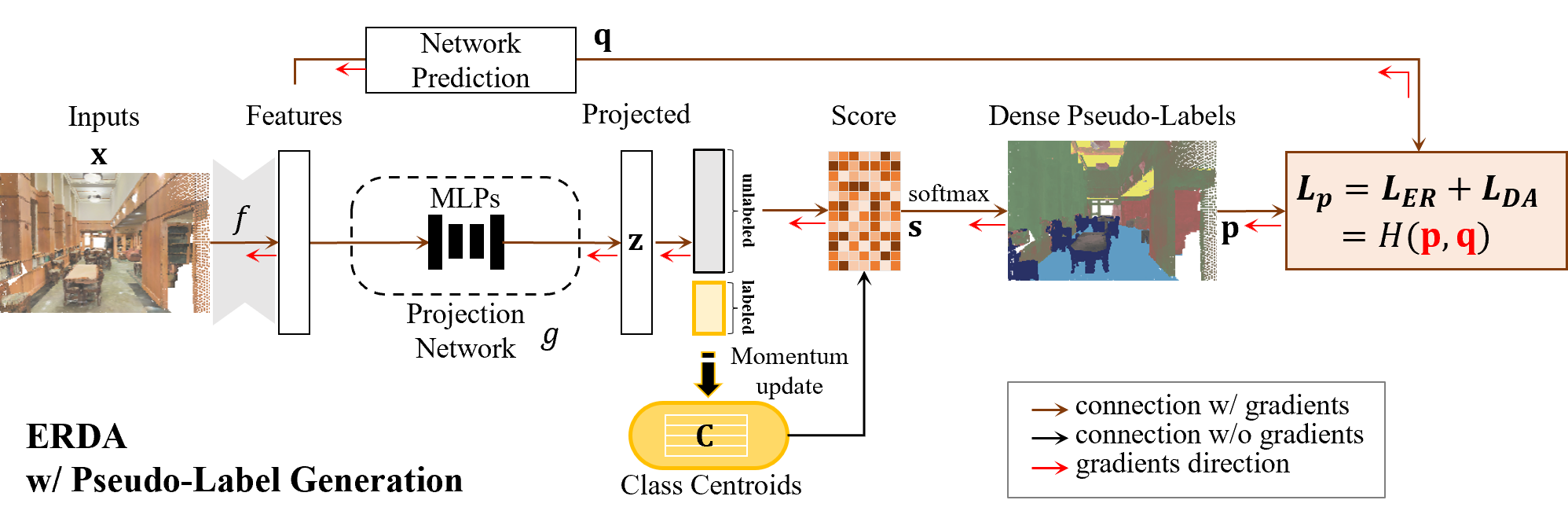
Figure 2: Detailed illustration of our ERDA with the prototypical pseudo-label generation process, which is shared for both (a) and (b) in Fig. 1.

4 Experiments

We present the benefits of our proposed ERDA by experimenting with multiple large-scale datasets, including S3DIS s3dis , ScanNet scannet , SensatUrban sensat and Pascal pascal . We also provide ablation studies for better investigation.

4.1 Experimental Setup

We choose RandLA-Net randlanet and CloserLook3D closerlook as our primary baselines following previous works. Additionally, while transformer models vit ; swin have revolutionized the field of computer vision as well as 3D point cloud segmentation pttransformer ; stratified , none of the existing works have addressed the training of transformer for point cloud segmentation with weak supervision, even though these models are known to be data-hungry vit . We thus further incorporate the PointTransformer (PT) pttransformer as our baseline to study the amount of supervision demanded for effective training of transformer.

For training, we follow the setup of the baselines and set the loss weight $\alpha=0.1$. For a fair comparison, we follow previous works weak_color ; weak_psd ; weak_sqn and experiment with different settings, including the 0.02% (1pt), 1% and 10% settings, where the available labels are randomly sampled according to the ratio. More details are given in the supplementary.

4.2 Performance Comparison

settings	methods	mIoU	ceiling	floor	wall	beam	column	window	door	table	chair	sofa	bookcase	board	clutter
Fully	PointNet pointnet	41.1	88.8	97.3	69.8	0.1	3.9	46.3	10.8	59.0	52.6	5.9	40.3	26.4	33.2
	MinkowskiNet Minkowski	65.4	91.8	98.7	86.2	0.0	34.1	48.9	62.4	81.6	89.8	47.2	74.9	74.4	58.6
	KPConv kpconv	65.4	92.6	97.3	81.4	0.0	16.5	54.5	69.5	90.1	80.2	74.6	66.4	63.7	58.1
	SQN weak_sqn	63.7	92.8	96.9	81.8	0.0	25.9	50.5	65.9	79.5	85.3	55.7	72.5	65.8	55.9
	HybridCR weak_hybrid	65.8	93.6	98.1	82.3	0.0	24.4	59.5	66.9	79.6	87.9	67.1	73.0	66.8	55.7
	RandLA-Net randlanet	64.6	92.4	96.8	80.8	0.0	18.6	57.2	54.1	87.9	79.8	74.5	70.2	66.2	59.3
	+ ERDA	68.3	93.9	98.5	83.4	0.0	28.9	62.6	70.0	89.4	82.7	75.5	69.5	75.3	58.7
	CloserLook3D closerlook	66.2	94.2	98.1	82.7	0.0	22.2	57.6	70.4	91.2	81.2	75.3	61.7	65.8	60.4
	+ ERDA	69.6	94.5	98.5	85.2	0.0	31.1	57.3	72.2	91.7	83.6	77.6	74.8	75.8	62.1
	PT pttransformer	70.4	94.0	98.5	86.3	0.0	38.0	63.4	74.3	89.1	82.4	74.3	80.2	76.0	59.3
	+ ERDA	72.6	95.8	98.6	86.4	0.0	43.9	61.2	81.3	93.0	84.5	77.7	81.5	74.5	64.9
0.02% (1pt)	zhang et al. weak_color	45.8	-	-	-	-	-	-	-	-	-	-	-	-	-
	PSD weak_psd	48.2	87.9	96.0	62.1	0.0	20.6	49.3	40.9	55.1	61.9	43.9	50.7	27.3	31.1
	MIL-Trans weak_mil	51.4	86.6	93.2	75.0	0.0	29.3	45.3	46.7	60.5	62.3	56.5	47.5	33.7	32.2
	HybridCR weak_hybrid	51.5	85.4	91.9	65.9	0.0	18.0	51.4	34.2	63.8	78.3	52.4	59.6	29.9	39.0
	RandLA-Net randlanet	40.6	84.0	94.2	59.0	0.0	5.4	40.4	16.9	52.8	51.4	52.2	16.9	27.8	27.0
	+ ERDA	48.4	87.3	96.3	61.9	0.0	11.3	45.9	31.7	73.1	65.1	57.8	26.1	36.0	36.4
	CloserLook3D closerlook	34.6	33.6	40.5	52.4	0.0	21.1	25.4	35.5	48.9	48.9	53.9	23.8	35.3	30.1
	+ ERDA	52.0	90.0	96.7	70.2	0.0	21.5	45.8	41.9	76.0	65.5	56.1	51.5	30.6	30.9
	PT pttransformer	2.2	0.0	0.0	29.2	0.0	0.0	0.0	0.0	0.0	0.0	0.0	0.0	0.0	0.0
	+ ERDA	26.2	86.8	96.9	63.2	0.0	0.0	0.0	15.1	29.6	26.3	0.0	0.0	0.0	22.8
1%	zhang et al. weak_color	61.8	91.5	96.9	80.6	0.0	18.2	58.1	47.2	75.8	85.7	65.2	68.9	65.0	50.2
	PSD weak_psd	63.5	92.3	97.7	80.7	0.0	27.8	56.2	62.5	78.7	84.1	63.1	70.4	58.9	53.2
	SQN weak_sqn	63.6	92.0	96.4	81.3	0.0	21.4	53.7	73.2	77.8	86.0	56.7	69.9	66.6	52.5
	HybridCR weak_hybrid	65.3	92.5	93.9	82.6	0.0	24.2	64.4	63.2	78.3	81.7	69.0	74.4	68.2	56.5
	RandLA-Net randlanet	59.8	92.3	97.5	77.0	0.1	15.9	48.7	38.0	83.2	78.0	68.4	62.4	64.9	50.6
	+ ERDA	67.2	94.2	97.5	82.3	0.0	27.3	60.7	68.8	88.0	80.6	76.0	70.5	68.7	58.4
	CloserLook3D closerlook	59.9	95.3	98.4	78.7	0.0	14.5	44.4	38.1	84.9	79.0	69.5	67.8	53.9	54.1
	+ ERDA	68.2	94.0	98.2	83.8	0.0	30.2	56.7	62.7	91.0	80.8	75.4	80.2	74.5	58.3
	PT pttransformer	65.8	94.2	98.2	83.0	0.0	44.2	50.4	68.8	88.1	83.0	75.2	47.4	64.3	59.0
	+ ERDA	70.4	95.5	98.1	85.5	0.0	30.5	61.7	73.3	90.1	82.6	77.6	80.6	76.0	63.1
10%	Xu and Lee weak_10few	48.0	90.9	97.3	74.8	0.0	8.4	49.3	27.3	69.0	71.7	16.5	53.2	23.3	42.8
	Semi-sup weak_cl	57.7	-	-	-	-	-	-	-	-	-	-	-	-	-
	zhang et al. weak_color	64.0	-	-	-	-	-	-	-	-	-	-	-	-	-
	SQN weak_sqn	64.7	93.0	97.5	81.5	0.0	28.0	55.8	68.7	80.1	87.7	55.2	72.3	63.9	57.0
	RandLA-Net randlanet	61.7	91.7	97.8	79.4	0.0	28.4	50.8	45.5	85.2	81.3	70.3	57.1	63.8	51.8
	+ ERDA	67.9	94.3	98.4	83.2	0.0	30.5	60.7	67.4	88.8	83.2	74.5	68.8	72.4	60.4
	CloserLook3D closerlook	55.5	93.0	98.2	73.6	0.0	12.6	25.6	33.3	87.5	72.9	65.1	73.1	36.0	51.1
	+ ERDA	69.1	94.7	98.5	83.2	0.0	28.8	53.8	70.9	91.5	82.5	75.8	82.1	75.3	61.6
	PT pttransformer	66.0	93.7	98.3	83.7	0.0	35.0	48.1	70.9	88.3	81.9	73.2	60.3	67.3	57.2
	+ ERDA	71.7	94.6	98.5	86.5	0.0	49.7	61.3	82.4	89.8	84.3	78.0	70.5	74.1	62.4

Table 2: The results are obtained on the S3DIS datasets Area 5. For all baseline methods, we follow their official instructions in evaluation. The bold denotes the best performance in each setting.

Results on S3DIS.

S3DIS s3dis is a large-scale point cloud segmentation dataset that covers 6 large indoor areas with 272 rooms and 13 semantic categories. As shown in Tab. 2, ERDA significantly improves over different baselines on all settings and almost all classes. In particular, for confusing classes such as column, window, door, and board, our method provides noticeable and consistent improvements in all weak supervision settings. We also note that PT suffers from severe over-fitting and feature collapsing under the supervision of extremely sparse labels of “1pt” setting; whereas it is alleviated with ERDA, though not achieving a satisfactory performance. Such observation agrees with the understanding that transformer is data-hungry vit .

Impressively, ERDA yields competitive performance against most supervised methods. For instance, with only $1\%$ of labels, it achieves performance better than its stand-alone baselines with full supervision. Such result indicates that the ERDA is more successful than expected in alleviating the lack of training signals, as also demonstrated qualitatively in Fig. 3.

Therefore, we further extend the proposed method to fully-supervised training, i.e., in setting “Fully” in Tab. 2. More specifically, we generate pseudo-labels for all points and regard the ERDA as an auxiliary loss for fully-supervised learning. Surprisingly, we observe non-trivial improvements (+3.7 for RandLA-Net and +3.4 for CloserLook3D) and achieve the state-of-the-art performance of 72.6 (+2.2) in mIoU with PT. We suggest that the improvements are due to the noise-aware learning from ERDA, which gradually reduces the noise during the model learning and demonstrates to be generally effective. Moreover, considering that the ground-truth labels could suffer from the problem of label noise noise_2d_pencil ; noise_3d_robust ; noise_survey , we also hypothesize that pseudo-labels from ERDA learning could stabilize fully-supervised learning and provide unexpected benefits.

We also conduct the 6-fold cross-validation, as reported in Tab. 6. We find our method achieves a leading performance among both weakly and fully-supervised methods, which further validates the effectiveness of our method.

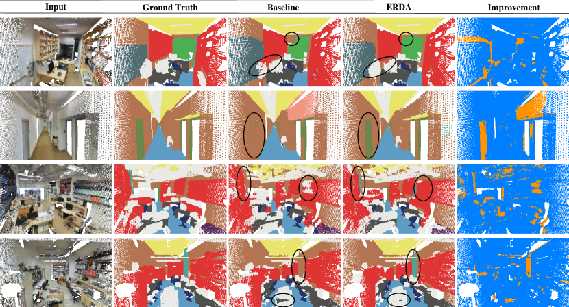
Figure 3: We show obvious improvement of our ERDA over baseline (RandLA-Net) on different scenes from S3DIS Area 5. In the office and hallway (top 2), ERDA produces more detailed and complete segmentation for windows and doors, and avoids over-expansion of the board and bookcase on the wall, thanks to the informative pseudo-labels. In more cluttered scenes (bottom 2), ERDA tends to make cleaner predictions by avoiding improper situations such as desk inside clutter and preserving important semantic classes such as columns.

settings	methods	mIoU
Fully	PointNet pointnet	47.6
	RandLA-Net randlanet	70.0
	KPConv kpconv	70.6
	HybridCR weak_hybrid	70.7
	PT pttransformer	73.5
	PointNeXt - XL pointnext	74.9
	RandLA-Net + ERDA	71.0
	CloserLook3D + ERDA	73.7
	PT + ERDA	76.3
1%	zhang et al. weak_color	65.9
	PSD weak_psd	68.0
	HybridCR weak_hybrid	69.2
	RandLA-Net + ERDA	69.4
	CloserLook3D + ERDA	72.3
	PT + ERDA	73.5

Table 3: Results on S3DIS 6-fold.

settings	methods	mIoU
Fully	PointCNN pointcnn	45.8
	RandLA-Net randlanet	64.5
	KPConv kpconv	68.4
	HybridCR weak_hybrid	59.9
	CloserLook3D + ERDA	70.4
20pts	MIL-Trans weak_mil	54.4
	CloserLook3D + ERDA	57.0
0.1%	SQN weak_sqn	56.9
	RandLA-Net + ERDA	62.0
1%	zhang et al. weak_color	51.1
	PSD weak_psd	54.7
	HybridCR weak_hybrid	56.8
	RandLA-Net + ERDA	63.0

Table 4: Results on ScanNet test.

settings	methods	mIoU
Fully	PointNet pointnet	23.7
	PointNet++ pointnet++	32.9
	RandLA-Net randlanet	52.7
	KPConv kpconv	57.6
	LCPFormer lcpformer	63.4
	RandLA-Net + ERDA	64.7
0.1%	SQN weak_sqn	54.0
	RandLA-Net + ERDA	56.4

Table 5: Results on SensatUrban test.

methods	92	183	366	732	1464
FixMatch weak_2d_fixmatch	63.9	73.0	75.5	77.8	79.2
+ ERDA	73.5	74.9	78.0	78.5	80.1

Table 6: Results on Pascal dataset.

Results on ScanNet.

ScanNet scannet is an indoor point cloud dataset that covers 1513 training scenes and 100 test scenes with 20 classes. In addition to the common settings, e.g., 1% labels, it also provides official data efficient settings, such as 20 points, where for each scene there are a pre-defined set of 20 points with the ground truth label. We evaluate on both settings and report the results in Tab. 6. We largely improve the performance under $0.1\%$ and $1\%$ labels. In 20pts setting, we also employ a convolutional baseline (CloserLook3D) for a fair comparison. With no modification on the model, we surpass MIL-transformer weak_mil that additionally augments the backbone with transformer modules and multi-scale inference. Besides, we apply ERDA to baseline under fully-supervised setting and achieve competitive performance. These results also validate the ability of ERDA in providing effective supervision signals.

Results on SensatUrban.

SensatUrban sensat is an urban-scale outdoor point cloud dataset that covers the landscape from three UK cities. In Tab. 6, ERDA surpasses SQN weak_sqn under the same 0.1% setting as well as its fully-supervised baseline, and also largely improves under full supervision. It suggests that our method can be robust to different types of datasets and effectively exploits the limited annotations as well as the unlabeled points.

Generalizing to 2D Pascal.

As our ERDA does not make specific assumptions on the 3D data, we explore its potential in generalizing to similar 2D settings. Specifically, we study an important task of semi-supervised segmentation on image weak_2d_freematch ; weak_2d_unimatch ; weak_2d_softmatch and implement our method to the popular baseline, FixMatch weak_2d_fixmatch , which combines the pseudo-labels with weak-to-strong consistency and is shown to benefit from stronger augmentation weak_2d_unimatch . We use DeepLabv3+ 2d_deeplabv3 with ResNet-101 2d_resnet .

As in Tab. 6, we show that ERDA brings consistent improvement from low to high data regime, despite the existence of strong data augmentation and the very different data as well as setting. It thus indicates the strong generalization of our method. We also see that the improvement is less significant than the 3D cases. It might be because 2D data are more structured (e.g., pixels on a 2D grid) and are thus less noisy than the 3D point cloud.

4.3 Ablations and Analysis

	ER	DA	mIoU	ent.
baseline			59.8	-
+ pseudo-labels			63.3	2.49
+ ERDA	✓		65.1	2.26
		✓	66.1	2.44
	✓	✓	67.2	2.40

(a)

$L_{\text{DA}}~{}\backslash~{}\lambda$	0	1	2
-	-	65.1	66.3
$KL(\mathbf{p}||\mathbf{q})$	66.1	67.2	66.6
$KL(\mathbf{q}||\mathbf{p})$	66.1	65.9	65.2
$JS$	65.2	65.4	65.1
$MSE$	66.0	66.2	66.1

(b)

$k$	one-hot	soft	ERDA
64	63.1	62.8	64.5
500	63.0	62.3	64.1
1e3	63.3	63.5	65.5
1e4	63.0	62.9	65.6
dense	62.7	62.6	67.2

(c)

Table 7: Ablations on ERDA. If not specified, the model is RandLA-Net trained with ERDA as well as dense pseudo-labels on S3DIS under the 1% setting and reports in mIoU. Default settings are marked in gray.

We mainly consider the 1% setting and ablates in Tab. 7 to better investigate ERDA and make a more thorough comparison with the current pseudo-label generation paradigm. For more studies on hyper-parameters, please refer to the supplementary.

Individual effectiveness of ER and DA.

To validate our initial hypothesis, we study the individual effectiveness of $L_{ER}$ and $L_{DA}$ in LABEL:tbl:abl_erda. While the pseudo-labels essentially improve the baseline performance, we remove its label selection and one-hot conversion when adding the ER or DA term. We find that using ER alone can already be superior to the common pseudo-labels and largely reduce the entropy of pseudo-labels (ent.) as expected, which verifies that the pseudo-labels are noisy, and reducing these noises could be beneficial. The improvement with the DA term alone is even more significant, indicating that a large discrepancy is indeed existing between the pseudo-labels and model prediction and is hindering the model training. Lastly, by combining the two terms, we obtain the ERDA that reaches the best performance but with the entropy of its pseudo-labels larger than ER only and smaller than DA only. It thus also verifies that the DA term could be biased to uniform distribution and that the ER term is necessary.

Different choices of ER and DA.

Aside from the analysis in Sec. 3.2, we empirically compare the results under different choices of distance for $L_{DA}$ and $\lambda$ for $L_{ER}$. As in LABEL:tbl:abl_dist, the outstanding result justifies the choice of $KL(\mathbf{q}||\mathbf{p})$ with $\lambda=1$. Additionally, all different choices and combinations of ER and DA terms improve over the common pseudo-labels (63.3), which also validates the general motivation for ERDA.

Ablating label selection.

We explore in more detail how the model performance is influenced by the amount of exploitation on unlabeled points, as ERDA learning aims to enable full utilization of the unlabeled points. In particular, we consider three pseudo-labels types: common one-hot pseudo-labels, soft pseudo-labels ($\mathbf{p}$), and soft pseudo-labels with ERDA learning. To reduce the number of pseudo-labels, we select sparse but high-confidence pseudo-labels following a common top-$k$ strategy weak_color ; weak_otoc with various values of $k$ to study its influence. As in LABEL:tbl:abl_dense, ERDA learning significantly improves the model performance under all cases, enables the model to consistently benefit from more pseudo-labels, and thus neglects the need for label selection such as top-$k$ strategy, as also revealed in Fig. 1. Besides, using soft pseudo-labels alone can not improve but generally hinders the model performance, as one-hot conversion may also reduce the noise in pseudo-labels, which is also not required with ERDA.

5 Limitation and Future Work

While we mostly focus on weak supervision in this paper, our method also brings improvements under fully-supervised setting. We would then like to further explore the effectiveness and relationship of $L_{ER}$ and $L_{DA}$ under full supervision as a future work. Besides, despite promising results, our method, like other weak supervision approaches, assumes complete coverage of semantic classes in the available labels, which may not always hold in real-world cases. Point cloud segmentation with missing or novel classes should be explored as an important future direction.

6 Conclusion

In this paper, we study the weakly-supervised 3D point cloud semantic segmentation, which imposes the challenge of highly sparse labels. Though pseudo-labels are widely used, label selection is commonly employed to overcome the noise, but it also prevents the full utilization of unlabeled data. By addressing this, we propose a new learning scheme on pseudo-labels, ERDA, that reduces the noise, aligns to the model prediction, and thus enables comprehensive exploitation of unlabeled data for effective training. Experimental results show that ERDA outperforms previous methods in various settings and datasets. Notably, it surpasses its fully-supervised baselines and can be further generalized to full supervision as well as 2D images.

Acknowledgement.

This project is supported in part by ARC FL-170100117, and IC-190100031.

Appendix A Supplementary: Introduction

In this supplementary material, we provide more details regarding implementation details in Appendix B, more analysis of ERDA in Appendix C, full experimental results in Appendix D, and studies on parameters in Appendix E.

Appendix B Supplementary: Implementation and Training Details

For the RandLA-Net randlanet and CloserLook3D closerlook baselines, we follow the instructions in their released code for training and evaluation, which are here (RandLA-Net) and here (CloserLook3D), respectively. Especially, in CloserLook3Dcloserlook , there are several local aggregation operations and we use the “Pseudo Grid” (KPConv-like) one, which provides a neat re-implementation of the popular KPConv kpconv network (rigid version). For point transformer (PT) pttransformer , we follow their paper and the instructions in the code base that claims to have the official code (here). For FixMatch weak_2d_fixmatch , we use the publicly available implementation here.

Our code and pre-trained models will be released.

Appendix C Supplementary: Delving into ERDA with More Analysis

Following the discussion in Sec. 3, we study the impact of entropy regularization as well as different distance measurements from the perspective of gradient updates.

In particular, we study the gradient on the score of the $i$-th class i.e., $s_{i}$, and denote it as $g_{i}=\frac{\partial L_{p}}{\partial s_{i}}$. Given that $\frac{\partial p_{j}}{\partial s_{i}}=\mathbb{1}_{(i=j)}p_{i}-p_{i}p_{j}$, we have $g_{i}=p_{i}\sum_{j}p_{j}(\frac{\partial L_{p}}{\partial p_{i}}-\frac{\partial L_{p}}{\partial p_{j}})$. As shown in Tab. 8, we demonstrate the gradient update $\Delta=-g_{i}$ under different situations.

In addition to the analysis in Sec. 3.2, we find that, when $\mathbf{q}$ is certain, i.e., $\mathbf{q}$ approaching a one-hot vector, the update of our choice $KL(\mathbf{p}||\mathbf{q})$ would approach the infinity. We note that this could be hardly encountered since $\mathbf{q}$ is typically also the output of a softmax function. Instead, we would rather regard it as a benefit because it would generate effective supervision on those model predictions with high certainty, and the problem of gradient explosion could also be prevented by common operations such as gradient clipping.

In Fig. 5, we provide visualization for a more intuitive understanding on the impact of different formulations for $L_{DA}$ as well as their combination with $L_{ER}$. Specifically, we consider a simplified case of binary classification and visualize their gradient updates when $\lambda$ takes different values. We also visualize the gradient updates of $L_{ER}$. By comparing the gradient updates, we observe that only $KL(\mathbf{p}||\mathbf{q})$ with $\lambda=1$ can achieve small updates when $\mathbf{q}$ is close to uniform ($q=\frac{1}{2}$ under the binary case), and that there is a close-0 plateau as indicated by the sparse contour lines.

Additionally, we also find that, when increasing the $\lambda$, all distances, except the $KL(\mathbf{p}||\mathbf{q})$, are modulated to be similar to the updates of having $L_{ER}$ alone; whereas $KL(\mathbf{p}||\mathbf{q})$ can still produce effective updates, which may indicate that $KL(\mathbf{p}||\mathbf{q})$ is more robust to the $\lambda$.

Appendix D Supplementary: Full Results

We provide full results for the experiments reported in the main paper. For S3DIS s3dis , we provide the full results of S3DIS with 6-fold cross-validation in Tab. 12. For ScanNet scannet and SensatUrban sensat , we evaluate on their online test servers, which are here and here, and provide the full results in Tab. 12 and Tab. 12, respectively.

$\displaystyle L_{DA}$	$\displaystyle KL(\mathbf{p}||\mathbf{q})$	$\displaystyle KL(\mathbf{q}||\mathbf{p})$	$\displaystyle JS(\mathbf{p},\mathbf{q})$	$\displaystyle MSE(\mathbf{p},\mathbf{q})$
$\displaystyle L_{p}$	$\displaystyle H(\mathbf{p},\mathbf{q})-(1-\lambda)H(\mathbf{p})$	$\displaystyle H(\mathbf{q},\mathbf{p})-H(\mathbf{q})+\lambda H(\mathbf{p})$	$\displaystyle H(\frac{\mathbf{p}+\mathbf{q}}{2})-(\frac{1}{2}-\lambda)H(\mathbf{p})-\frac{1}{2}H(\mathbf{q})$	$\displaystyle\frac{1}{2}\sum_{i}(p_{i}-q_{i})^{2}+\lambda H(\mathbf{p})$
$\displaystyle g_{i}$	$\displaystyle p_{i}\sum_{j}p_{j}(-\log\frac{q_{i}}{q_{j}}+(1-\lambda)\log\frac{p_{i}}{p_{j}})$	$\displaystyle p_{i}-q_{i}-\lambda p_{i}\sum_{j}p_{j}\log\frac{p_{i}}{p_{j}}$	$\displaystyle p_{i}\sum_{j}p_{j}(\frac{-1}{2}\log\frac{p_{i}+q_{i}}{p_{j}+q_{j}}+(\frac{1}{2}-\lambda)\log\frac{p_{i}}{p_{j}})$	$\displaystyle p_{i}(p_{i}-q_{i})-p_{i}\sum_{j}p_{j}(p_{j}-q_{j})-\lambda p_{i}\sum_{j}p_{j}\log\frac{p_{i}}{p_{j}}$
Situations	$\displaystyle\Delta=-g_{i}$
$\displaystyle p_{k}\rightarrow 1$	$\displaystyle 0$	$\displaystyle q_{i}-\mathbb{1}_{k=i}$	$\displaystyle 0$	$\displaystyle 0$
$\displaystyle q_{1}=...=q_{K}$	$\displaystyle(\lambda-1)p_{i}\sum_{j}p_{j}\log\frac{p_{i}}{p_{j}}$	$\displaystyle\frac{1}{K}-p_{i}+\lambda p_{i}\sum_{j}p_{j}\log\frac{p_{i}}{p_{j}}$	$\displaystyle p_{i}\sum_{j\neq i}p_{j}(\frac{1}{2}\log\frac{Kp_{i}+1}{Kp_{j}+1}+(\lambda-\frac{1}{2})\log\frac{p_{i}}{p_{j}})$	$\displaystyle-p_{i}^{2}+p_{i}\sum_{j}p_{j}^{2}+\lambda p_{i}\sum_{j}p_{j}\log\frac{p_{i}}{p_{j}}$
$\displaystyle q_{i}\rightarrow 1$	$\displaystyle+\inf$	$\displaystyle 1-p_{i}+\lambda p_{i}\sum_{j}p_{j}\log\frac{p_{i}}{p_{j}}$	$\displaystyle p_{i}\sum_{j\neq i}p_{j}(\frac{1}{2}\log\frac{p_{i}+1}{p_{j}}+(\lambda-\frac{1}{2})\log\frac{p_{i}}{p_{j}})$	$\displaystyle-p_{i}^{2}+p_{i}(1-p_{i})+p_{i}\sum_{j}p_{j}^{2}+\lambda p_{i}\sum_{j}p_{j}\log\frac{p_{i}}{p_{j}}$
$\displaystyle q_{k\neq i}\rightarrow 1$	$\displaystyle-\inf$	$\displaystyle-p_{i}+\lambda p_{i}\sum_{j}p_{j}\log\frac{p_{i}}{p_{j}}$	$\displaystyle\displaystyle p_{i}\sum_{j\neq i}p_{j}(\frac{1}{2}\log\frac{p_{i}}{p_{j}+\mathbb{1}_{j=k}}+(\lambda-\frac{1}{2})\log\frac{p_{i}}{p_{j}})$	$\displaystyle-p_{i}^{2}-p_{i}p_{k}+p_{i}\sum_{j}p_{j}^{2}+\lambda p_{i}\sum_{j}p_{j}\log\frac{p_{i}}{p_{j}}$

Table 8: The formulation of $L_{p}$ using different functions to formulate $L_{DA}$. We present the gradients $g_{i}=\frac{\partial L_{p}}{\partial s_{i}}$, and the corresponding update $\Delta=-g_{i}$ under different situations. Analysis can be found in the Sec. 3.2 and Appendix C.

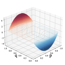
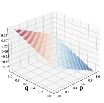
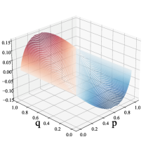
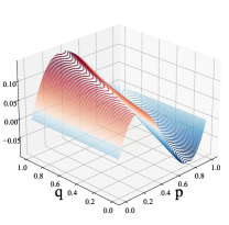
(a) $\lambda=0$

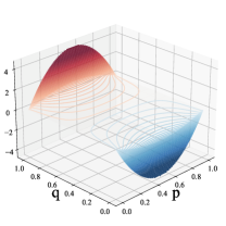
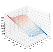
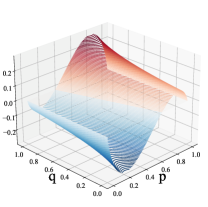
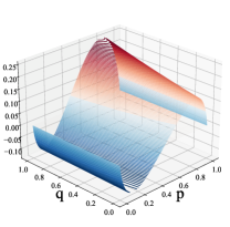
(b) $\lambda=1$

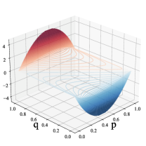
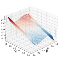
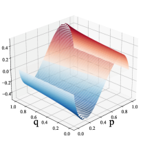
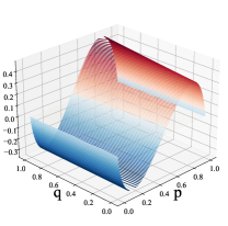
(c) $\lambda=2$

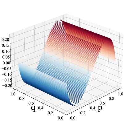
(d) Gradient updates of $L_{ER}$

Figure 5: Contour visualization of the gradient update with binary classes for better understanding. For a clearer view, we use red for positive updates and blue for negative updates, the darker indicates larger absolute values and the lighter indicates smaller absolute values.

Appendix E Supplementary: Ablations and Parameter Study

We further study the hyper-parameters involved in the implementation of ERDA with the prototypical pseudo-label generation, including loss weight $\alpha$, momentum coefficient $m$, and the use of projection network. As shown in Tab. 9, the proposed method acquires decent performance (mIoUs are all $>65$ and mostly $>66$) in a wide range of different hyper-parameter settings, compared with its fully-supervised baseline (64.7 mIoU) and previous state-of-the-art performance (65.3 mIoU by HybridCR weak_hybrid ).

Additionally, we suggest that the projection network could be effective in facilitating the ERDA learning, which can be learned to specialize in the pseudo-label generation task. This could also be related to the advances in contrastive learning. Many works simclr ; simclrv2 ; byol suggest that a further projection on feature representation can largely boost the performance because such projection decouples the learned features from the pretext task. We share a similar motivation in decoupling the features for ERDA learning on the pseudo-label generation task from the features for the segmentation task.

$m$	mIoU
0.9	66.19
0.99	66.80
0.999	67.18
0.9999	66.22

(a)

projection	mIoU
-	65.90
linear	66.55
2-layer MLPs	67.18
3-layer MLPs	66.31

(b)

$\alpha$	mIoU
0.001	65.25
0.01	66.01
0.1	67.18
1	65.95

(c)

Table 9: Parameter study on ERDA. If not specified, the model is RandLA-Net with ERDA trained with loss weight $\alpha=0.1$, momentum $m=0.999$, and 2-layer MLPs as projection networks under 1% setting on S3DIS. Default settings are marked in gray.

settings	methods	mIoU	ceiling	floor	wall	beam	column	window	door	table	chair	sofa	bookcase	board	clutter
Fully	RandLA-Net + ERDA	71.0	94.0	96.1	83.7	59.2	48.3	62.7	73.6	65.6	78.6	71.5	66.8	65.4	57.9
	CloserLook3D + ERDA	73.7	94.1	93.6	85.8	65.5	50.2	58.7	79.2	71.8	79.6	74.8	73.0	72.0	59.5
	PT + ERDA	76.3	94.9	97.8	86.2	65.4	55.2	64.1	80.9	84.8	79.3	74.0	74.0	69.3	66.2
1%	RandLA-Net + ERDA	69.4	93.8	92.5	81.7	60.9	43.0	60.6	70.8	65.1	76.4	71.1	65.3	65.3	55.0
	CloserLook3D + ERDA	72.3	94.2	97.5	84.1	62.9	46.2	59.2	73.0	71.5	77.0	73.6	71.0	67.7	61.2
	PT + ERDA	73.5	94.9	97.7	85.3	66.7	53.2	60.9	80.8	69.2	78.4	73.3	67.7	65.9	62.1

Table 10: The full results of ERDA with different baselines on S3DIS 6-fold cross-validation.

settings	methods	mIoU	bathtub	bed	books.	cabinet	chair	counter	curtain	desk	door	floor	other	pic	fridge	shower	sink	sofa	table	toilet	wall	wndw
Fully	CloserLook3D + ERDA	70.4	75.9	76.2	77.0	68.2	84.3	48.1	81.3	62.1	61.4	94.7	52.7	19.9	57.1	88.0	75.9	79.9	64.7	89.2	84.2	66.6
20pts	CloserLook3D + ERDA	57.0	75.1	62.5	63.1	46.0	77.7	30.0	64.9	46.1	43.6	93.3	36.0	15.4	38.0	73.6	51.6	69.5	47.2	83.2	74.5	47.8
0.1%	RandLA-Net + ERDA	62.0	75.7	72.4	67.9	56.9	79.0	31.8	73.0	58.1	47.3	94.1	47.1	15.2	46.3	69.2	51.8	72.8	56.5	83.2	79.2	62.0
1%	RandLA-Net + ERDA	63.0	63.2	73.1	66.5	60.5	80.4	40.9	72.9	58.5	42.4	94.3	50.0	35.0	53.0	57.0	60.4	75.6	61.9	78.8	73.8	62.6

Table 11: The full results of ERDA with different baselines on ScanNet scannet test set, obtained from its online benchmark site by the time of submission.

settings	methods	mIoU	OA	Ground	Vegetation	Buildings	Walls	Bridge	Parking	Rail	Roads	Street Furniture	Cars	Footpath	Bikes	Water
Fully	RandLA-Net + ERDA	64.7	93.1	86.1	98.1	95.2	64.7	66.9	59.6	49.2	62.5	46.5	85.8	45.1	0.0	81.5
0.1%	RandLA-Net + ERDA	56.4	91.1	82.0	97.4	93.2	56.4	57.1	53.1	5.2	60.0	33.6	81.2	39.9	0.0	74.2

Table 12: The full results of ERDA with different baselines on SensatUrban sensat test set, obtained from its online benchmark site by the time of submission.

References

- (1) Jiwoon Ahn and Suha Kwak. Learning pixel-level semantic affinity with image-level supervision for weakly supervised semantic segmentation. 2018 IEEE/CVF Conference on Computer Vision and Pattern Recognition, pages 4981–4990, 2018.
- (2) Iro Armeni, Sasha Sax, Amir R Zamir, and Silvio Savarese. Joint 2d-3d-semantic data for indoor scene understanding. arXiv preprint arXiv:1702.01105, 2017.
- (3) Alexandre Boulch, Gilles Puy, and Renaud Marlet. Fkaconv: Feature-kernel alignment for point cloud convolution, 2020.
- (4) A. Boulch, B. Le Saux, and N. Audebert. Unstructured point cloud semantic labeling using deep segmentation networks. In Proceedings of the Workshop on 3D Object Retrieval, 3Dor ’17, page 17–24, Goslar, DEU, 2017. Eurographics Association.
- (5) Mathilde Caron, Ishan Misra, Julien Mairal, Priya Goyal, Piotr Bojanowski, and Armand Joulin. Unsupervised learning of visual features by contrasting cluster assignments. ArXiv, abs/2006.09882, 2020.
- (6) Mathilde Caron, Hugo Touvron, Ishan Misra, Herve Jegou, Julien Mairal, Piotr Bojanowski, and Armand Joulin. Emerging properties in self-supervised vision transformers. 2021 IEEE/CVF International Conference on Computer Vision (ICCV), Oct 2021.
- (7) Chen Chen, Zhe Chen, Jing Zhang, and Dacheng Tao. Sasa: Semantics-augmented set abstraction for point-based 3d object detection. In AAAI, 2022.
- (8) Hao Chen, Ran Tao, Yue Fan, Yidong Wang, Jindong Wang, Bernt Schiele, Xing Xie, Bhiksha Raj, and Marios Savvides. Softmatch: Addressing the quantity-quality trade-off in semi-supervised learning. 2023.
- (9) Liang-Chieh Chen, Yukun Zhu, George Papandreou, Florian Schroff, and Hartwig Adam. Encoder-decoder with atrous separable convolution for semantic image segmentation. In European Conference on Computer Vision, 2018.
- (10) Ting Chen, Simon Kornblith, Mohammad Norouzi, and Geoffrey Hinton. A simple framework for contrastive learning of visual representations. arXiv preprint arXiv:2002.05709, 2020.
- (11) Ting Chen, Simon Kornblith, Kevin Swersky, Mohammad Norouzi, and Geoffrey Hinton. Big self-supervised models are strong semi-supervised learners. arXiv preprint arXiv:2006.10029, 2020.
- (12) Zhe Chen, Jing Zhang, and Dacheng Tao. Progressive lidar adaptation for road detection. IEEE/CAA Journal of Automatica Sinica, 6:693–702, 05 2019.
- (13) Mingmei Cheng, Le Hui, Jin Xie, and Jian Yang. Sspc-net: Semi-supervised semantic 3d point cloud segmentation network. 2021.
- (14) Julian Chibane, Francis Engelmann, Tuan Anh Tran, and Gerard Pons-Moll. Box2mask: Weakly supervised 3d semantic instance segmentation using bounding boxes. Computer Vision - ECCV 2022, pages 681–699, 2022.
- (15) Christopher Choy, JunYoung Gwak, and Silvio Savarese. 4d spatio-temporal convnets: Minkowski convolutional neural networks. In Proceedings of the IEEE Conference on Computer Vision and Pattern Recognition, pages 3075–3084, 2019.
- (16) Angela Dai, Angel X. Chang, Manolis Savva, Maciej Halber, Thomas Funkhouser, and Matthias Nießner. Scannet: Richly-annotated 3d reconstructions of indoor scenes. In Proc. Computer Vision and Pattern Recognition (CVPR), IEEE, 2017.
- (17) Alexey Dosovitskiy, Lucas Beyer, Alexander Kolesnikov, Dirk Weissenborn, Xiaohua Zhai, Thomas Unterthiner, Mostafa Dehghani, Matthias Minderer, Georg Heigold, Sylvain Gelly, Jakob Uszkoreit, and Neil Houlsby. An image is worth 16x16 words: Transformers for image recognition at scale. ICLR, 2021.
- (18) Oren Dovrat, Itai Lang, and Shai Avidan. Learning to sample. 2019 IEEE/CVF Conference on Computer Vision and Pattern Recognition (CVPR), Jun 2019.
- (19) M. Everingham, S. M. A. Eslami, L. Van Gool, C. K. I. Williams, J. Winn, and A. Zisserman. The pascal visual object classes challenge: A retrospective. International Journal of Computer Vision, 111(1):98–136, Jan. 2015.
- (20) Zhengyang Feng, Qianyu Zhou, Qiqi Gu, Xin Tan, Guangliang Cheng, Xuequan Lu, Jianping Shi, and Lizhuang Ma. Dmt: Dynamic mutual training for semi-supervised learning. Pattern Recognition, 130:108777, Oct 2022.
- (21) Biao Gao, Yancheng Pan, Chengkun Li, Sibo Geng, and Huijing Zhao. Are we hungry for 3d lidar data for semantic segmentation? a survey of datasets and methods. IEEE Transactions on Intelligent Transportation Systems, 23(7):6063–6081, Jul 2022.
- (22) Benjamin Graham, Martin Engelcke, and Laurens van der Maaten. 3d semantic segmentation with submanifold sparse convolutional networks. 2018 IEEE/CVF Conference on Computer Vision and Pattern Recognition, Jun 2018.
- (23) Benjamin Graham and Laurens van der Maaten. Submanifold sparse convolutional networks. ArXiv, abs/1706.01307, 2017.
- (24) Yves Grandvalet and Yoshua Bengio. Semi-supervised learning by entropy minimization. In L. Saul, Y. Weiss, and L. Bottou, editors, Advances in Neural Information Processing Systems, volume 17. MIT Press, 2004.
- (25) Jean-Bastien Grill, Florian Strub, Florent Altch’e, Corentin Tallec, Pierre H. Richemond, Elena Buchatskaya, Carl Doersch, Bernardo Ávila Pires, Zhaohan Daniel Guo, Mohammad Gheshlaghi Azar, Bilal Piot, Koray Kavukcuoglu, Rémi Munos, and Michal Valko. Bootstrap your own latent: A new approach to self-supervised learning. ArXiv, abs/2006.07733, 2020.
- (26) Meng-Hao Guo, Junxiong Cai, Zheng-Ning Liu, Tai-Jiang Mu, Ralph R. Martin, and Shi-Min Hu. PCT: point cloud transformer. CoRR, abs/2012.09688, 2020.
- (27) Yulan Guo, Hanyun Wang, Qingyong Hu, Hao Liu, Li Liu, and Mohammed Bennamoun. Deep learning for 3d point clouds: A survey. IEEE transactions on pattern analysis and machine intelligence, 2020.
- (28) Lei Han, Tian Zheng, Lan Xu, and Lu Fang. Occuseg: Occupancy-aware 3d instance segmentation. 2020 IEEE/CVF Conference on Computer Vision and Pattern Recognition (CVPR), pages 2937–2946, 2020.
- (29) Kaiming He, Haoqi Fan, Yuxin Wu, Saining Xie, and Ross Girshick. Momentum contrast for unsupervised visual representation learning. arXiv preprint arXiv:1911.05722, 2019.
- (30) K. He, X. Zhang, S. Ren, and J. Sun. Deep residual learning for image recognition. In 2016 IEEE Conference on Computer Vision and Pattern Recognition (CVPR), pages 770–778, Los Alamitos, CA, USA, jun 2016. IEEE Computer Society.
- (31) Ruifei He, Jihan Yang, and Xiaojuan Qi. Re-distributing biased pseudo labels for semi-supervised semantic segmentation: A baseline investigation. In Proceedings of the IEEE/CVF International Conference on Computer Vision, pages 6930–6940, 2021.
- (32) Qingyong Hu, Bo Yang, Guangchi Fang, Yulan Guo, Ales Leonardis, Niki Trigoni, and Andrew Markham. Sqn: Weakly-supervised semantic segmentation of large-scale 3d point clouds. In European Conference on Computer Vision, 2022.
- (33) Qingyong Hu, Bo Yang, Sheikh Khalid, Wen Xiao, Niki Trigoni, and Andrew Markham. Sensaturban: Learning semantics from urban-scale photogrammetric point clouds. International Journal of Computer Vision, 130(2):316–343, 2022.
- (34) Qingyong Hu, Bo Yang, Linhai Xie, Stefano Rosa, Yulan Guo, Zhihua Wang, Niki Trigoni, and Andrew Markham. Randla-net: Efficient semantic segmentation of large-scale point clouds. CoRR, abs/1911.11236, 2019.
- (35) Zeyu Hu, Mingmin Zhen, Xuyang Bai, Hongbo Fu, and Chiew-Lan Tai. Jsenet: Joint semantic segmentation and edge detection network for 3d point clouds. CoRR, abs/2007.06888, 2020.
- (36) Zhuo Huang, Zhiyou Zhao, Banghuai Li, and Jungong Han. Lcpformer: Towards effective 3d point cloud analysis via local context propagation in transformers. ArXiv, abs/2210.12755, 2022.
- (37) Li Jiang, Shaoshuai Shi, Zhuotao Tian, Xin Lai, Shu Liu, Chi-Wing Fu, and Jiaya Jia. Guided point contrastive learning for semi-supervised point cloud semantic segmentation. In ICCV, pages 6403–6412, 10 2021.
- (38) Yi Kun and Wu Jianxin. Probabilistic End-to-end Noise Correction for Learning with Noisy Labels. In The IEEE Conference on Computer Vision and Pattern Recognition (CVPR), 2019.
- (39) Abhijit Kundu, Xiaoqi Yin, Alireza Fathi, David A. Ross, Brian Brewington, Thomas A. Funkhouser, and Caroline Pantofaru. Virtual multi-view fusion for 3d semantic segmentation. In ECCV, 2020.
- (40) Hyeokjun Kweon and Kuk-Jin Yoon. Joint learning of 2d-3d weakly supervised semantic segmentation. In Alice H. Oh, Alekh Agarwal, Danielle Belgrave, and Kyunghyun Cho, editors, Advances in Neural Information Processing Systems, 2022.
- (41) Donghyeon Kwon and Suha Kwak. Semi-supervised semantic segmentation with error localization network. In Proceedings of the IEEE/CVF Conference on Computer Vision and Pattern Recognition (CVPR), pages 9957–9967, June 2022.
- (42) Xin Lai, Jianhui Liu, Li Jiang, Liwei Wang, Hengshuang Zhao, Shu Liu, Xiaojuan Qi, and Jiaya Jia. Stratified transformer for 3d point cloud segmentation. 2022 IEEE/CVF Conference on Computer Vision and Pattern Recognition (CVPR), pages 8490–8499, 2022.
- (43) Yuxiang Lan, Yachao Zhang, Yanyun Qu, Cong Wang, Chengyang Li, Jia Cai, Yuan Xie, and Zongze Wu. Weakly supervised 3d segmentation via receptive-driven pseudo label consistency and structural consistency. Proceedings of the AAAI Conference on Artificial Intelligence, 37(1):1222–1230, Jun. 2023.
- (44) L. Landrieu and M. Simonovsky. Large-scale point cloud semantic segmentation with superpoint graphs. In 2018 IEEE/CVF Conference on Computer Vision and Pattern Recognition, pages 4558–4567, 2018.
- (45) Felix Järemo Lawin, Martin Danelljan, Patrik Tosteberg, Goutam Bhat, Fahad Shahbaz Khan, and Michael Felsberg. Deep projective 3d semantic segmentation. Lecture Notes in Computer Science, page 95–107, 2017.
- (46) Dong-Hyun Lee. Pseudo-label : The simple and efficient semi-supervised learning method for deep neural networks. 2013.
- (47) Mengtian Li, Yuan Xie, Yunhang Shen, Bo Ke, Ruizhi Qiao, Bo Ren, Shaohui Lin, and Lizhuang Ma. Hybridcr: Weakly-supervised 3d point cloud semantic segmentation via hybrid contrastive regularization. In Proceedings of the IEEE/CVF Conference on Computer Vision and Pattern Recognition (CVPR), pages 14930–14939, June 2022.
- (48) Yangyan Li, Rui Bu, Mingchao Sun, Wei Wu, Xinhan Di, and Baoquan Chen. Pointcnn: Convolution on x-transformed points. In S. Bengio, H. Wallach, H. Larochelle, K. Grauman, N. Cesa-Bianchi, and R. Garnett, editors, Advances in Neural Information Processing Systems, volume 31. Curran Associates, Inc., 2018.
- (49) Di Lin, Jifeng Dai, Jiaya Jia, Kaiming He, and Jian Sun. Scribblesup: Scribble-supervised convolutional networks for semantic segmentation. 2016 IEEE Conference on Computer Vision and Pattern Recognition (CVPR), pages 3159–3167, 2016.
- (50) Yuyuan Liu, Yu Tian, Yuanhong Chen, Fengbei Liu, Vasileios Belagiannis, and Gustavo Carneiro. Perturbed and strict mean teachers for semi-supervised semantic segmentation. 2022 IEEE/CVF Conference on Computer Vision and Pattern Recognition (CVPR), Jun 2022.
- (51) Ze Liu, Han Hu, Yue Cao, Zheng Zhang, and Xin Tong. A closer look at local aggregation operators in point cloud analysis. ECCV, 2020.
- (52) Ze Liu, Yutong Lin, Yue Cao, Han Hu, Yixuan Wei, Zheng Zhang, Stephen Lin, and Baining Guo. Swin transformer: Hierarchical vision transformer using shifted windows. arXiv preprint arXiv:2103.14030, 2021.
- (53) Zhengzhe Liu, Xiaojuan Qi, and Chi-Wing Fu. One thing one click: A self-training approach for weakly supervised 3d semantic segmentation. CoRR, abs/2104.02246, 2021.
- (54) Tao Lu, Limin Wang, and Gangshan Wu. Cga-net: Category guided aggregation for point cloud semantic segmentation. In Proceedings of the IEEE/CVF Conference on Computer Vision and Pattern Recognition (CVPR), pages 11693–11702, June 2021.
- (55) A. Milioto, I. Vizzo, J. Behley, and C. Stachniss. Rangenet++: Fast and accurate lidar semantic segmentation. In 2019 IEEE/RSJ International Conference on Intelligent Robots and Systems (IROS), pages 4213–4220, 2019.
- (56) Charles Ruizhongtai Qi, Hao Su, Kaichun Mo, and Leonidas J. Guibas. Pointnet: Deep learning on point sets for 3d classification and segmentation. CoRR, abs/1612.00593, 2016.
- (57) Charles Ruizhongtai Qi, Li Yi, Hao Su, and Leonidas J. Guibas. Pointnet++: Deep hierarchical feature learning on point sets in a metric space. CoRR, abs/1706.02413, 2017.
- (58) Guocheng Qian, Yuchen Li, Houwen Peng, Jinjie Mai, Hasan Hammoud, Mohamed Elhoseiny, and Bernard Ghanem. Pointnext: Revisiting pointnet++ with improved training and scaling strategies. In Advances in Neural Information Processing Systems (NeurIPS), 2022.
- (59) Haibo Qiu, Baosheng Yu, and Dacheng Tao. Collect-and-distribute transformer for 3d point cloud analysis. arXiv preprint arXiv:2306.01257, 2023.
- (60) Mamshad Nayeem Rizve, Kevin Duarte, Yogesh S Rawat, and Mubarak Shah. In defense of pseudo-labeling: An uncertainty-aware pseudo-label selection framework for semi-supervised learning. In International Conference on Learning Representations, 2021.
- (61) Claude Elwood Shannon. A mathematical theory of communication. The Bell System Technical Journal, 27:379–423, 1948.
- (62) Hanyu Shi, Jiacheng Wei, Ruibo Li, Fayao Liu, and Guosheng Lin. Weakly supervised segmentation on outdoor 4d point clouds with temporal matching and spatial graph propagation. In 2022 IEEE/CVF Conference on Computer Vision and Pattern Recognition (CVPR), pages 11830–11839, 2022.
- (63) Jake Snell, Kevin Swersky, and Richard Zemel. Prototypical networks for few-shot learning. In Advances in Neural Information Processing Systems, 2017.
- (64) Kihyuk Sohn, David Berthelot, Nicholas Carlini, Zizhao Zhang, Han Zhang, Colin A Raffel, Ekin Dogus Cubuk, Alexey Kurakin, and Chun-Liang Li. Fixmatch: Simplifying semi-supervised learning with consistency and confidence. In H. Larochelle, M. Ranzato, R. Hadsell, M.F. Balcan, and H. Lin, editors, Advances in Neural Information Processing Systems, volume 33, pages 596–608. Curran Associates, Inc., 2020.
- (65) Hwanjun Song, Minseok Kim, Dongmin Park, Yooju Shin, and Jae-Gil Lee. Learning from noisy labels with deep neural networks: A survey. IEEE Transactions on Neural Networks and Learning Systems, pages 1–19, 2022.
- (66) Liyao Tang, Yibing Zhan, Zhe Chen, Baosheng Yu, and Dacheng Tao. Contrastive boundary learning for point cloud segmentation. In 2022 IEEE/CVF Conference on Computer Vision and Pattern Recognition (CVPR), pages 8479–8489, 2022.
- (67) Lyne Tchapmi, Christopher Choy, Iro Armeni, JunYoung Gwak, and Silvio Savarese. Segcloud: Semantic segmentation of 3d point clouds. 2017 International Conference on 3D Vision (3DV), Oct 2017.
- (68) Hugues Thomas, Charles R. Qi, Jean-Emmanuel Deschaud, Beatriz Marcotegui, François Goulette, and Leonidas J. Guibas. Kpconv: Flexible and deformable convolution for point clouds. CoRR, abs/1904.08889, 2019.
- (69) Ozan Unal, Dengxin Dai, and Luc Van Gool. Scribble-supervised lidar semantic segmentation. ArXiv, abs/2203.08537, 2022.
- (70) Guo-Hua Wang and Jianxin Wu. Repetitive reprediction deep decipher for semi-supervised learning. Proceedings of the AAAI Conference on Artificial Intelligence, 34(04):6170–6177, Apr. 2020.
- (71) Peng-Shuai Wang, Yang Liu, Yu-Xiao Guo, Chun-Yu Sun, and Xin Tong. O-CNN: Octree-based Convolutional Neural Networks for 3D Shape Analysis. ACM Transactions on Graphics (SIGGRAPH), 36(4), 2017.
- (72) Yidong Wang, Hao Chen, Qiang Heng, Wenxin Hou, Yue Fan, , Zhen Wu, Jindong Wang, Marios Savvides, Takahiro Shinozaki, Bhiksha Raj, Bernt Schiele, and Xing Xie. Freematch: Self-adaptive thresholding for semi-supervised learning. 2023.
- (73) Yuxi Wang, Junran Peng, and Zhaoxiang Zhang. Uncertainty-aware pseudo label refinery for domain adaptive semantic segmentation. In 2021 IEEE/CVF International Conference on Computer Vision (ICCV), pages 9072–9081, 2021.
- (74) Yue Wang, Yongbin Sun, Ziwei Liu, Sanjay E. Sarma, Michael M. Bronstein, and Justin M. Solomon. Dynamic graph CNN for learning on point clouds. CoRR, abs/1801.07829, 2018.
- (75) Yuchao Wang, Haochen Wang, Yujun Shen, Jingjing Fei, Wei Li, Guoqiang Jin, Liwei Wu, Rui Zhao, and Xinyi Le. Semi-supervised semantic segmentation using unreliable pseudo-labels. ArXiv, abs/2203.03884, 2022.
- (76) Zongji Wang and Feng Lu. Voxsegnet: Volumetric cnns for semantic part segmentation of 3d shapes. IEEE transactions on visualization and computer graphics, 2018.
- (77) Jiacheng Wei, Guosheng Lin, Kim-Hui Yap, Tzu-Yi Hung, and Lihua Xie. Multi-path region mining for weakly supervised 3d semantic segmentation on point clouds. In Proceedings of the IEEE/CVF Conference on Computer Vision and Pattern Recognition, pages 4384–4393, 2020.
- (78) Wenxuan Wu, Zhongang Qi, and Fuxin Li. Pointconv: Deep convolutional networks on 3d point clouds. CoRR, abs/1811.07246, 2018.
- (79) Xiaoyang Wu, Yixing Lao, Li Jiang, Xihui Liu, and Hengshuang Zhao. Point transformer v2: Grouped vector attention and partition-based pooling. In NeurIPS, 2022.
- (80) Zhonghua Wu, Yicheng Wu, Guosheng Lin, and Jianfei Cai. Reliability-adaptive consistency regularization for weakly-supervised point cloud segmentation, 2023.
- (81) Zhonghua Wu, Yicheng Wu, Guosheng Lin, Jianfei Cai, and Chen Qian. Dual adaptive transformations for weakly supervised point cloud segmentation. arXiv preprint arXiv:2207.09084, 2022.
- (82) Qizhe Xie, Minh-Thang Luong, Eduard Hovy, and Quoc V Le. Self-training with noisy student improves imagenet classification. arXiv preprint arXiv:1911.04252, 2019.
- (83) Y. Xie, J. Tian, and X. X. Zhu. Linking points with labels in 3d: A review of point cloud semantic segmentation. IEEE Geoscience and Remote Sensing Magazine, 8(4):38–59, 2020.
- (84) Chenfeng Xu, Bichen Wu, Zining Wang, Wei Zhan, Peter Vajda, Kurt Keutzer, and Masayoshi Tomizuka. Squeezesegv3: Spatially-adaptive convolution for efficient point-cloud segmentation. ArXiv, abs/2004.01803, 2020.
- (85) Xun Xu and Gim Hee Lee. Weakly supervised semantic point cloud segmentation: Towards 10x fewer labels. In CVPR, 2020.
- (86) Xu Yan, Chaoda Zheng, Zhen Li, Sheng Wang, and Shuguang Cui. Pointasnl: Robust point clouds processing using nonlocal neural networks with adaptive sampling. CoRR, abs/2003.00492, 2020.
- (87) Cheng-Kun Yang, Ji-Jia Wu, Kai-Syun Chen, Yung-Yu Chuang, and Yen-Yu Lin. An mil-derived transformer for weakly supervised point cloud segmentation. In Proceedings of the IEEE/CVF Conference on Computer Vision and Pattern Recognition (CVPR), pages 11830–11839, June 2022.
- (88) Jiancheng Yang, Qiang Zhang, Bingbing Ni, Linguo Li, Jinxian Liu, Mengdie Zhou, and Qi Tian. Modeling point clouds with self-attention and gumbel subset sampling. CoRR, abs/1904.03375, 2019.
- (89) Lihe Yang, Lei Qi, Litong Feng, Wayne Zhang, and Yinghuan Shi. Revisiting weak-to-strong consistency in semi-supervised semantic segmentation. In CVPR, 2023.
- (90) Shuquan Ye, Dongdong Chen, Songfang Han, and Jing Liao. Learning with noisy labels for robust point cloud segmentation. International Conference on Computer Vision, 2021.
- (91) Bowen Zhang, Yidong Wang, Wenxin Hou, Hao Wu, Jindong Wang, Manabu Okumura, and Takahiro Shinozaki. Flexmatch: Boosting semi-supervised learning with curriculum pseudo labeling. 2021.
- (92) Pan Zhang, Bo Zhang, Ting Zhang, Dong Chen, and Fang Wen. Robust mutual learning for semi-supervised semantic segmentation, 2021.
- (93) Xiaolong Zhang, Zuqiang Su, Xiaolin Hu, Yan Han, and Shuxian Wang. Semisupervised momentum prototype network for gearbox fault diagnosis under limited labeled samples. IEEE Transactions on Industrial Informatics, 18(9):6203–6213, 2022.
- (94) Yachao Zhang, Zonghao Li, Yuan Xie, Yanyun Qu, Cuihua Li, and Tao Mei. Weakly supervised semantic segmentation for large-scale point cloud. In Proceedings of the AAAI Conference on Artificial Intelligence, volume 35, pages 3421–3429, 2021.
- (95) Yachao Zhang, Yanyun Qu, Yuan Xie, Zonghao Li, Shanshan Zheng, and Cuihua Li. Perturbed self-distillation: Weakly supervised large-scale point cloud semantic segmentation. In Proceedings of the IEEE/CVF International Conference on Computer Vision, pages 15520–15528, 2021.
- (96) Yan Zhang, Wenhan Zhao, Bo Sun, Ying Zhang, and Wen Wen. Point cloud upsampling algorithm: A systematic review. Algorithms, 15(4), 2022.
- (97) Hengshuang Zhao, Li Jiang, Jiaya Jia, Philip Torr, and Vladlen Koltun. Point transformer, 2021.
- (98) Zhedong Zheng and Yi Yang. Rectifying pseudo label learning via uncertainty estimation for domain adaptive semantic segmentation. International Journal of Computer Vision, 129(4):1106–1120, Jan 2021.
- (99) Bolei Zhou, Aditya Khosla, Àgata Lapedriza, Aude Oliva, and Antonio Torralba. Learning deep features for discriminative localization. 2016 IEEE Conference on Computer Vision and Pattern Recognition (CVPR), pages 2921–2929, 2016.
- (100) Yanning Zhou, Hang Xu, Wei Zhang, Bin Gao, and Pheng-Ann Heng. C3-semiseg: Contrastive semi-supervised segmentation via cross-set learning and dynamic class-balancing. In 2021 IEEE/CVF International Conference on Computer Vision (ICCV), pages 7016–7025, 2021.