section subsection

HIGHLY SMOOTH ZEROTH-ORDER METHODS FOR SOLVING
OPTIMIZATION PROBLEMS UNDER THE PL CONDITION

Abstract – In this paper, we study the black box optimization problem under the Polyak–Lojasiewicz (PL) condition, assuming that the objective function is not just smooth, but has higher smoothness. By using "kernel-based’’ approximations instead of the exact gradient in the Stochastic Gradient Descent method, we improve the best-known results of convergence in the class of gradient-free algorithms solving problems under the PL condition. We generalize our results to the case where a zeroth-order oracle returns a function value at a point with some adversarial noise. We verify our theoretical results on the example of solving a system of nonlinear equations.

Keywords: Black-box optimization, gradient-free methods, kernel approximation, maximum noise level.

1.   Introduction

The black box problem is a fundamental optimization problem when the objective function has only a zero-order oracle [1]. Recently, this problem has received significant attention in the setting of reinforcement learning [2, 3], federated learning [4, 5], and deep learning [6, 7]. Particularly in applied problems of multi-armed bandit [8, 9], online optimization [10, 11, 12], huge-scale optimization [13, 14], and hyperparameter tuning [15, 16]. In addition, the black box problem arises if the information about the derivatives is too expensive or not available [17].

To solve such problems in the convex case, there are various techniques for developing optimal gradient-free algorithms based on first-order optimization algorithms, optimal by three criteria at once: oracle complexity, iteration complexity, and maximum level of admissible noise still allowing to guarantee certain accuracy [18]. The main idea of which is to calculate the gradient approximation instead of an exact gradient [19]. For example, $L_{1}$, and $L_{2}$ randomized approximations [20, 21, 8, 22, 12] and "kernel-based" approximation [23, 11, 24, 25] are usually used for the smooth case. Where the "kernel-based" approximation takes advantage of higher-order smoothness as opposed to the $L_{2}$ and $L_{1}$ randomized approximations. For the non-smooth case, there are smoothing techniques via $L_{1}$ and $L_{2}$ randomized approximation [26, 5].

In contrast to the convex case, where algorithms have been intensively appearing and being studied in theory and practice in recent years [[, e.g.,]and see above]Karimireddy_2018, the analysis of the black box problem in the nonconvex case is just beginning to be actively studied [28, 29, 30]. One such problem that is frequently common in the literature lately is the smooth (nonconvex) optimization problem under the Polyak–Lojasiewicz condition [31, 32, 33, 34, 35]. In this formulation of the problem, [36] studied the biased Stochastic Gradient Descent (SGD) method and also proposed its gradient-free counterpart.

We focus on solving the smooth black-box optimization problem (in particular, the nonconvex optimization) under the Polyak–Lojasiewicz condition. We propose an optimal zero-order algorithm (see Algorithm 1) based on Mini-batch SGD (added batching to biased Stochastic Gradient Descent [36] to improve iteration complexity). Using kernel approximation as a technique for developing a gradient-free algorithm, we show in theory and in practice a significant improvement in convergence rate estimates. We provide an extended analysis of Algorithm 1, namely we consider a (close to reality) stochastic formulation of the problem with adversarial noise [37, 38, 39].

Table 1: Comparison of convergence results of Zero-Order Mini-batch SGD method via Kernel-based approximation, "Kernel approx." (This work) with the existing counterpart via Gaussian approximation, "Gaus. approx." [36]. Notation: $d$ = dimension, $\delta(x)$ = adversarial deterministic noise, $\xi$ = adversarial stochastic noise, $\Delta$ = level noise, $\beta$ = smoothness order parameter.

Case	Zero-order oracle	Error floor		Stochastic?	Adversarial noise
		Gaussian approx.	Kernel approx.		ADN?	ASN?
deterministic	$\tilde{f}(x)=f(x)+\delta(x)$	$\mathcal{O}\left(d^{2}\Delta\right)$	$\mathcal{O}\left(d^{2}\Delta^{{\color[rgb]{0,0,1}\frac{2(\beta-1)}{\beta}}}\right)$	✗	✓	✗
two-point	$\tilde{f}(x,\xi)=f(x,\xi)+\delta(x)$	$\mathcal{O}\left(d^{2}\Delta\right)$	$\mathcal{O}\left(d^{2}\Delta^{{\color[rgb]{0,0,1}\frac{2(\beta-1)}{\beta}}}\right)$	✓	✓	✗
one-point	$\tilde{f}(x,\xi)=f(x)+\xi$	$\varepsilon$	$\varepsilon$	✓	✗	✓
	$\tilde{f}(x,\xi)=f(x)+\xi+\delta(x)$	$\mathcal{O}\left(d^{2}\Delta\right)$	$\mathcal{O}\left(d^{2}\Delta^{{\color[rgb]{0,0,1}\frac{2(\beta-1)}{\beta}}}\right)$	✓	✓	✓

1.1.   Contribution

• We present a Zero-Order Mini-batch SGD method that significantly improves existing estimates of the convergence results (in particular, estimates of the error floor, see the "deterministic" case of the zero-order oracle (first line) in Table 1 and Table 2) in a class of gradient-free algorithms for solving smooth nonconvex problems under the PL condition.

• We provide an extended theoretical analysis of the Zero-Order Mini-batch SGD algorithm by considering a stochastic setting using a gradient approximation with one-point and two-point feedback, when the zero-order oracle is corrupted by an bounded adversarial deterministic ("ADN") and stochastic ("ASN") noise. We show that also in the stochastic setting a Zero-Order Mini-batch Stochastic Gradient Descent method is superior to the existing counterpart [36] (see stochastic cases of the zero-order oracle $\tilde{f}(x,\xi)$ in Table 1 and Table 2).

• We empirically verify our theoretical results by comparing the Zero-Order Mini-batch Stochastic Gradient Descent method with the existing algorithm using a typical example for problems under the Polyak–Lojasiewicz condition: solving a system of nonlinear equations.

• We demonstrate the effectiveness of the randomized approximation in practice by comparing it to the Gaussian approximation from [36] and show the advantages of "kernel-based" approximation in experiments by additionally comparing it to the $L_{2}$ approximation.

1.2.   Paper organization

This article has the following structure. In Section 2 we provide related works. We describe the statement of the problem in Section 3. We present the optimal gradient-free Algorithm 1 in Section 4. In Section 5, we extend our analysis of the Algorithm 1 to a stochastic setting with different models of adversarial noise. In Section 7, we discuss the results. While in Section 8 we analyze the effectiveness of our approach on a practical experiment. Section 9 concludes the paper. We give a detailed proof of the Theorems and Lemmas in the Appendix (Supplementary Materials).

Table 2: Comparison of iteration complexity #$N$ oracle complexity, #$T$ and maximum noise level #$\Delta$ of the algorithm with the following approaches: Kernel and Gaussian approximations for zero-order oracle cases ① : $\tilde{f}(x)=f(x)+\delta(x)$, ② : $\tilde{f}(x,\xi)=f(x,\xi)+\delta(x)$, ③ : $\tilde{f}(x,\xi)=f(x)+\xi$, ④ : $\tilde{f}(x,\xi)=f(x)+\xi+\delta(x)$. In both approaches, the dependence of the estimates on the batch size $B$ is presented. Notation: $\beta$ = order of smoothness, $\varepsilon$ = accuracy of the solution to the problem, $d$ = dimension, $\mu$ = Polyak–Lojasiewicz condition constant.

Case	Batch	Gaussian approximation				Kernel approximation
	Size	# $N$	# $T$	# $\Delta$		# $N$	# $T$	# $\Delta$
①, ②, ④	$B\in[1,\beta^{3}d]$	$\tilde{\mathcal{O}}\left(\frac{d}{B}\mu^{-1}\right)$	$\tilde{\mathcal{O}}\left(d\mu^{-1}\right)$	$\Delta\leq\mu\varepsilon d^{-3/2}$		$\tilde{\mathcal{O}}\left(\frac{d}{B}\mu^{-1}\right)$	$\tilde{\mathcal{O}}\left(d\mu^{-1}\right)$	$\Delta\leq\mu\varepsilon d^{-3/2}$
	$B>\beta^{3}d$	$\tilde{\mathcal{O}}\left(\mu^{-1}\right)$	$\max\left\{\tilde{\mathcal{O}}\left(\mu^{-1}B\right),\tilde{\mathcal{O}}\left(\frac{d^{4}\Delta^{2}}{\varepsilon^{2}\mu^{3}}\right)\right\}$	$\Delta\leq\mu\varepsilon d^{-2}$		$\tilde{\mathcal{O}}\left(\mu^{-1}\right)$	$\max\left\{\tilde{\mathcal{O}}\left(\mu^{-1}B\right),\tilde{\mathcal{O}}\left(\frac{d^{2+\frac{2}{\beta-1}}\Delta^{2}}{\varepsilon^{\frac{\beta}{\beta-1}}\mu^{\frac{2\beta-1}{\beta-1}}}\right)\right\}$	$\Delta\leq\frac{\left(\mu\varepsilon\right)^{\frac{\beta}{2(\beta-1)}}}{d^{\frac{\beta}{\beta-1}}}$
③	$B\in[1,\beta^{3}d]$	$\tilde{\mathcal{O}}\left(\frac{d}{B}\mu^{-1}\right)$	$\tilde{\mathcal{O}}\left(d\mu^{-1}\right)$	$\Delta\leq\mu\varepsilon d^{-1}$		$\tilde{\mathcal{O}}\left(\frac{d}{B}\mu^{-1}\right)$	$\tilde{\mathcal{O}}\left(d\mu^{-1}\right)$	$\Delta\leq\mu\varepsilon d^{-1}$
	$B>\beta^{3}d$	$\tilde{\mathcal{O}}\left(\mu^{-1}\right)$	$\max\left\{\tilde{\mathcal{O}}\left(\mu^{-1}B\right),\tilde{\mathcal{O}}\left(\frac{d^{4}\Delta^{2}}{\varepsilon^{2}\mu^{3}}\right)\right\}$	$\Delta\leq\mu\varepsilon d^{-2}B^{1/2}$		$\tilde{\mathcal{O}}\left(\mu^{-1}\right)$	$\max\left\{\tilde{\mathcal{O}}\left(\mu^{-1}B\right),\tilde{\mathcal{O}}\left(\frac{d^{2+\frac{2}{\beta-1}}\Delta^{2}}{\varepsilon^{\frac{\beta}{\beta-1}}\mu^{\frac{2\beta-1}{\beta-1}}}\right)\right\}$	$\Delta\leq\frac{\left(\mu\varepsilon\right)^{\frac{\beta}{2(\beta-1)}}}{d^{\frac{\beta}{\beta-1}}}B^{1/2}$

2.   Related Work

Polyak–Lojasiewicz condition.

The field of research on the nonconvex problem under the Polyak–Lojasiewicz condition can be traced back to [31], where it is shown that this condition is sufficient for the gradient descent to achieve a global linear convergence rate. Recently, problems with Polyak–Lojasiewicz condition have been actively investigated. For instance, [35] proposed a new formulation of the problem under the Polyak–Lojasiewicz condition, including a compromise and an early stopping rule to guarantee its achievement. Already in the new statement of the problem, [40] proposed a fully adaptive gradient algorithm (with respect to the Lipschitz constant of the gradient and the noise level in the gradient) for solving problems with this condition. However, in this work we consider the standard statement of the problem under the Polyak–Lojasiewicz condition [[, e.g. see]]Karimi_2016, Yue_2022. Also, it is shown in [41] that non-accelerated algorithms are optimal for smooth problems under the Polyak–Lojasiewicz condition. Therefore, in this paper, we consider non-accelerated first-order optimization algorithms as a base for developing optimal gradient-free methods.

SGD type algorithms.

Many works [42, 43, 44, 45, 46, 47] investigated Stochastic Gradient Descent in various settings. For black-box problems, this algorithm and its modifications are the basis for developing gradient-free algorithms. For instance, [5] used the following first-order optimization algorithms as a basis for developing gradient-free algorithms in the federated learning setting: Minibatch Accelerated SGD and Single-Machine Accelerated SGD [[, from ]]Woodworth_2021, and Federated Accelerated Stochastic Gradient Descent [[, from ]]Yuan_2020, which are accelerated modifications of the SGD, namely the AC-SA [50]. In a nonconvex optimization problem with a Polyak–Lojasiewicz condition, [36] studied a biased Stochastic Gradient Descent, where the oracle has access to biased and noisy gradient estimates, and showed that Stochastic Gradient Descent methods can generally converge only to the neighborhood of the solution. In this paper, we use the biased Stochastic Gradient Descent algorithm [36] as a basis for developing an optimal zero-order method for solving a smooth nonconvex optimization problem, assuming that the Polyak–Lojasiewicz condition is satisfied.

Kernel approximation.

The works [23, 11, 24, 25] investigated and used kernel approximation as a technique for creating gradient-free algorithms. In the survey [18] showed that the significant difference of this approximation from others is taking into account the advantages of the high order of smoothness of the objective function, i.e. satisfying the Hölder condition. All these works [11, 24, 25] used the central finite difference (CFD) scheme instead of the forward finite difference scheme (FFD) in kernel approximation. It turns out there is an explanation, [51] showed that in a smooth case, one should use CFD, not FFD. In this paper, we use the kernel approximation since we assume that our function has higher smoothness, in contrast to [36], where only smoothness is assumed.

Stochastic optimization.

Stochastic optimization problems have received special attention in the literature [46, 52, 53, 54, 55, 56]. For example, [57] investigated a stochastic problem with non-sub-Gaussian (heavy-tailed) noise in the convex case, and [56] investigated in the convex-concave case. For black-box problems, [24, 25] studied a one-point gradient approximation with additive stochastic noise. [58] studied a two-point gradient approximation corrupted by an adversarial deterministic noise, and [5] studied a one-point gradient approximation with the same adversarial deterministic noise. In this paper, we generalize our analysis to the stochastic optimization problem and consider gradient approximation with one-point and two-point feedback obtained via function realizations. We consider two cases of noise: noise as defined in [24, 25, 12] and noise as defined in [26, 58].

To the best of our knowledge for the moment there are lack of results around gradient-free methods for problems with Polyak–Lojasiewicz condition. The known results [59, 60, 61] are dominated by [36] as we consider to be state of the art results.

3.   Setup

We study black-box optimization problems of the form:

$$f^{*}:=\min_{x\in Q\subset\mathbb{R}^{d}}f(x),$$ (1)

where $f:\mathbb{R}^{d}\rightarrow\mathbb{R}$ is a function that we want to minimize over a closed convex subset $Q$ of $\mathbb{R}^{d}$. The problem (1) is a general statement problem in the field of optimization. In order to narrow down the class of problems to be solved, let us define the function class using the following assumptions.

3.1.   Notation

We use $\langle x,y\rangle:=\sum_{i=1}^{d}x_{i}y_{i}$ to denote standard inner product of $x,y\in\mathbb{R}^{d}$. We denote $l_{p}$ - norms ($p\leavevmode\nobreak\ \geq\leavevmode\nobreak\ 1$) in $\mathbb{R}^{d}$ as $\|x\|_{p}:=\left(\sum_{i=1}^{d}|x_{i}|^{p}\right)^{1/p}$. Particularly, for $l_{2}$-norm in $\mathbb{R}^{d}$ it follows $\|x\|_{2}\leavevmode\nobreak\ :=\leavevmode\nobreak\ \sqrt{\langle x,x\rangle}$. We denote $l_{p}$-sphere as $S_{p}^{d}(r):=\left\{x\in\mathbb{R}^{d}:\|x\|_{p}=r\right\}$. Operator $\mathbb{E}[\cdot]$ denotes full mathematical expectation. We use the notation $\tilde{O}(\cdot)$ to hide logarithmic factors.

3.2.   Assumptions on the objective function

For all our theoretical results we assume that $f$ is not just smooth, but has a high order of smoothness.

Assumption 1 (Higher order smoothness)

Let $l$ denote the maximal integer number strictly less than $\beta$. Let $\mathcal{F}_{\beta}(L)$ denote the set of all functions $f:\mathbb{R}^{d}\rightarrow\mathbb{R}$ which are differentiable $l$ times and for all $x,z\in Q$ the Hölder-type condition holds:

$$\left|f(z)-\sum_{0\leq|n|\leq l}\frac{1}{n!}D^{n}f(x)(z-x)^{n}\right|\leq L_{\beta}\|z-x\|^{\beta}_{2},$$

where $L_{\beta}>0$, the sum is over multi-index $n\leavevmode\nobreak\ =\leavevmode\nobreak\ (n_{1},...,n_{d})\in\mathbb{N}^{d}$, we used the notation $n!\leavevmode\nobreak\ =\leavevmode\nobreak\ n_{1}!\cdots n_{d}!$, $|n|=n_{1}+\cdots+n_{d}$, and $\forall v=(v_{1},...,v_{d})\in\mathbb{R}^{d}$ we defined

$$D^{n}f(x)v^{n}=\frac{\partial^{|n|}f(x)}{\partial^{n_{1}}x_{1}\cdots\partial^{n_{d}}x_{d}}v_{1}^{n_{1}}\cdots v_{d}^{n_{d}}.$$

Also we assume the Polyak–Lojasiewicz condition ($\mu$-PL) with parameter $\mu>0$.

Assumption 2 ($\mu$-PL)

The function is differentiable and there exists constant $\mu>0$ s.t. $\forall x\in\mathbb{R}^{d}$

$$\|\nabla f(x)\|^{2}_{2}\geq 2\mu(f(x)-f^{*}).$$ (2)

Assumption 1 is quite common in the literature [[, e.g.]]Bach_2016,Tsybakov_2020,Novitskii_2021. We introduced this assumption in order to take advantage of the properties of higher smoothness. As far as we know Assumption 2 was introduced by [31]. Functions satisfying this assumption are called gradient-dominated functions [62].

3.3.   Assumptions on the biased gradient oracle

We now formulate the standard assumptions about the gradient oracle for the biased SGD method [36]. To do this, we start by introducing the following definition.

Definition 1 (Biased Gradient Oracle)

A map $\mathbf{g}\leavevmode\nobreak\ :\leavevmode\nobreak\ \mathbb{R}^{d}\leavevmode\nobreak\ \times\leavevmode\nobreak\ \mathcal{D}\rightarrow\mathbb{R}^{d}$ s.t.

$$\mathbf{g}(x,\xi)=\nabla f(x)+\mathbf{b}(x)+\mathbf{n}(x,\xi)$$ (3)

for a bias $\mathbf{b}:\mathbb{R}^{d}\rightarrow\mathbb{R}^{d}$ and zero-mean noise $\mathbf{n}:\mathbb{R}^{d}\times\mathcal{D}\rightarrow\mathbb{R}^{d}$, that is $\mathbb{E}_{\xi}\mathbf{n}(x,\xi)=0,\forall x\in\mathbb{R}^{d}$.

We assume that this gradient oracle has bias and noise, and they are bounded.

Assumption 3 (($M,\sigma^{2}$)-bounded noise)

There exists constants $M,\sigma^{2}\geq 0$ such that $\forall x\in\mathbb{R}^{d}$

$$\mathbb{E}_{\xi}\|\mathbf{n}(x,\xi)\|^{2}_{2}\leq M\|\nabla f(x)+\mathbf{b}(x)\|^{2}_{2}+\sigma^{2}.$$ (4)

Assumption 4 (Bounded bias)

There exists constants $0\leq m<1$, and $\zeta^{2}\geq 0$ s.t. $\forall x\in\mathbb{R}^{d}$

$$\|\mathbf{b}(x)\|^{2}_{2}\leq m\|\nabla f(x)\|^{2}_{2}+\zeta^{2}.$$ (5)

Many prior work in the context stochastic optimization often assumed the bounded noise and bounded bias. For example, the Assumption 3 is similar as in [46]. In the case without bias, Assumption 3 is referred to as the strong growth condition [[, e.g. ]]Vaswani_2019. Also the Assumption 4 was used by [64].

The assumptions introduced in this subsection are necessary to use the following auxiliary lemma, since our approach to creating a gradient-free method is based on the SGD algorithm [36] (see Appendix C).

Lemma 1

Let $\{x_{k}\}_{k\geq 0}$ denote the iterates of Algorithm SGD [36] with batching, function $f$ satisfy Assumptions 1-2 with $\beta=2$, and the gradient oracle (3) satisfy Assumptions 3-4. Then there exists step size $\eta\leavevmode\nobreak\ \leq\leavevmode\nobreak\ \frac{1}{(M+1)L_{2}}$ such that it holds for all $N\geq 0$ and an arbitrary batch size $B$

$$\mathbb{E}[f(x_{N})]-f^{*}\leq(1-\eta\mu(1-m))^{N}(f(x_{0})-f^{*})+\frac{\zeta^{2}}{2\mu(1-m)}+\frac{\eta L_{2}\sigma^{2}}{2B\mu(1-m)}.$$

4.   Zero-Order Mini-batch SGD

In this section, we present our approach to solving problem (1) when the gradient oracle (3) has no information about the derivatives of the objective function. The main idea of our approach is to create an optimal (on oracle complexity, iteration complexity, and maximum level of noise) gradient-free algorithm based on the first-order method (namely, Stochastic Gradient Descent). To begin, we introduce an approximation of the gradient oracle (3) via a zero-order oracle (value of the objective function $f(x)$ with some adversarial deterministic noise $\delta(x)$ such that $|\delta(x)|\leq\Delta$ and $\Delta>0$):

$$\tilde{f}(x)=f(x)+\delta(x),$$ (6)

which take advantage of the higher smoothness of the function [11, 24, 25]. Such approximation is referred to as "kernel-based" approximation of gradient and has the following form

$$\mathbf{\tilde{g}}(x,\mathbf{e})=d\frac{\tilde{f}(x+\gamma r\mathbf{e})-\tilde{f}(x-\gamma r\mathbf{e})}{2\gamma}K(r)\mathbf{e},$$ (7)

where $\gamma>0$ is smoothing parameter, $\mathbf{e}$ is uniformly distributed in $S_{2}^{d}(1)$, $r$ is uniformly distributed in $[-1,1]$, $\mathbf{e}$ and $r$ are independent, $K:\leavevmode\nobreak\ [-1,1]\leavevmode\nobreak\ \rightarrow\leavevmode\nobreak\ \mathbb{R}$ is a kernel function that satisfies

$$\mathbb{E}[K(u)]=0,\;\;\;\mathbb{E}[uK(u)]=1,\;\;\;\mathbb{E}[u^{j}K(u)]=0,\;\;\;j=2,...,l,\;\;\;\mathbb{E}[|u|^{\beta}|K(u)|]<\infty.$$

Now we can present Algorithm 1. This algorithm is a modification of SGD method. Instead of calculating the first-order gradient oracle from Definition 1, we calculate an approximation of the gradient (7). Also, to achieve an optimal iteration complexity, we add a batch size $B$.

Algorithm 1 Zero-Order Mini-batch Stochastic Gradient Descent (ZO-MB-SGD)

  Input: step size $\eta$, iteration number $N$, batch size $B$, Kernel $K:[-1,1]\rightarrow\mathbb{R}$, smoothing parameter $\gamma$, $x_{0}\leavevmode\nobreak\ \in\leavevmode\nobreak\ \mathbb{R}^{d}$

  for $k=0$ to $N-1$ do

       1.    Sample vectors $\mathbf{e}_{1},\mathbf{e}_{2}...,\mathbf{e}_{B}$ uniformly distributed on the unit sphere $S_{2}^{d}(1)$ and scalars

       1.    $r_{1},r_{2},...,r_{B}$ uniformly distributed on the interval [-1, 1]

       2.    Define $\tilde{\mathbf{g}}(x_{k},\mathbf{e}_{i})=d\frac{\tilde{f}(x_{k}+\gamma r_{i}\mathbf{e}_{i})-\tilde{f}(x_{k}-\gamma r_{i}\mathbf{e}_{i})}{2\gamma}K(r_{i})\mathbf{e}_{i}$ using (6)

       3.    Calculate $\mathbf{g}_{k}=\frac{1}{B}\sum_{i=1}^{B}\tilde{\mathbf{g}}(x_{k},\mathbf{e}_{i})$

       4.    $x_{k+1}\leftarrow x_{k}-\eta\mathbf{g}_{k}$

  end for

  Return: $x_{N}$

The next theorem presents the convergence result of ZO-MB-SGD method in terms of the expectation.

Theorem 1

Let function $f(x)$ satisfy Assumptions 1 - 2 and the gradient approximation (7) satisfy Assumptions 3 - 4 then by choosing the step size $\eta\leavevmode\nobreak\ \leq\leavevmode\nobreak\ \frac{1}{(M+1)L_{2}}$, there exists parameters

$$\begin{split}&M\leq 6\beta^{3}d,\;\;\;\;\;\sigma^{2}\leq\frac{3\beta^{3}d^{2}L_{2}^{2}\gamma^{2}}{4}+\frac{2\beta^{3}d^{2}\Delta^{2}}{\gamma^{2}},\quad m=0,\;\;\;\;\;\;\zeta^{2}\leq\beta^{2}d^{2}\left(L_{\beta}^{2}\gamma^{2(\beta-1)}+\frac{\Delta^{2}}{\gamma^{2}}\right)\end{split}$$

such that Algorithm 1 with smoothing parameter $\gamma\leavevmode\nobreak\ \leq\leavevmode\nobreak\ \mathcal{O}\left(\Delta^{1/\beta}\right)$ achieves the following error floor

$$\mathbb{E}f(x_{N})-f^{*}=\max\left\{\varepsilon,\mathcal{O}\left(d^{2}\Delta^{\frac{2(\beta-1)}{\beta}}\right)\right\},$$

where $f^{*}$ is the solution to problem (1), $L_{2}$ is the Lipschitz gradient constant with respect to 2-norm.

The convergence result of Theorem 1 shows that Algorithm 1 with gradient approximation (7) achieves the error floor $\mathcal{O}\left(d^{2}\Delta^{\frac{2(\beta-1)}{\beta}}\right)$ with linear convergence rate. This asymptote arises due to the accumulation of adversarial noise in the bias $\mathbf{b}(x)$. To achieve $\varepsilon$-accuracy of Problem (1), the maximum level of noise can be defined as $\Delta\leq\mathcal{O}\left(\varepsilon^{\frac{\beta}{2(\beta-1)}}d^{\frac{-\beta}{\beta-1}}\right)$. This result significantly improves the approach described in [36]. Namely, using the same concept of the zero-order oracle (6) Algorithm 1 via Gaussian approximation achieves the error floor $\mathcal{O}\left(d^{2}\Delta\right)$, respectively, with the following maximum level of noise $\Delta\leq\mathcal{O}\left(\varepsilon d^{-2}\right)$. For a detailed proof of Theorem 1, see Appendix D. Also see Appendix H for details on estimates for Gaussian smoothing approximation.

Note that the results of Theorem 1 were obtained by using the deterministic setting of the zero-order oracle (6). However, if we reformulate problem (1) to a stochastic setting, specifying that $f(x):=\mathbb{E}_{\xi}f(x,\xi)$ and we use a gradient approximation (7) with two-point feedback, replacing in the zero-order oracle (6) the calculation of objective function value $f(x)$ with the calculation of objective function value on realizations $f(x,\xi)$, then it is not difficult to show that the convergence results of Theorem 1 also hold for Algorithm 1, which uses the gradient approximation with two-point feedback, where the term two-point feedback implies that it is possible to get the value of the objective function at two points on one realization. See Appendix E and I for a detailed proof of the case where Algorithm 1 uses a gradient approximation with two-point feedback, applying the "kernel-based" approximation and Gaussian approximation approaches, respectively. The concepts of a stochastic zero-order oracle when two-point feedback is not available are explored in the Section 5.

Remark 1

It should be noted that Algorithm 1 has a linear convergence rate (see Theorem 1). Then, since the ZO-MB-SGD method uses a randomized scheme (randomization on the $L_{2}$ sphere), we can obtain exact estimates of the large deviation probabilities using Markov’s inequality [65]:

$$\mathcal{P}\left(f(x_{N(\varepsilon\omega)})-f^{*}\geq\varepsilon\right)\leq\omega\frac{\mathbb{E}\left[f(x_{N(\varepsilon\omega)}\right]-f^{*}}{\varepsilon\omega}\leq\omega.$$

5.   Extended analysis of convergence via stochastic zero-order oracle

In this section, we continue our study of gradient-free methods for solving Problem (1) with the $\mu$-PL condition (see Assumption 2). We want to extend the analysis of Algorithm 1. Specifically, for cases where the zero-order oracle has a stochastic setting $\tilde{f}(x,\xi)$. To do this, we consider the concept of gradient approximation when only one-point feedback is available [[, see, e.g. ]]Gasnikov_2017 with two types of adversarial noise: adversarial stochastic noise, which is quite common in the following works [24, 25, 12], and adversarial deterministic noise, which is actively used in [58, 5, 26]. To introduce stochastic, let us rewrite the initial problem (1), where zero-order oracle returns an unbiased noisy stochastic function value $f(x,\xi)$:

$$\min_{x\in Q\subset\mathbb{R}^{d}}\{f(x):=\mathbb{E}_{\xi}f(x,\xi)\}.$$ (8)

5.1.   Stochastic zero-order oracle with additive adversarial stochastic noise

If for some reason two-point feedback is not available, you can use Zero-Order Mini-batch Stochastic Gradient Descent method (see Algorithm 1) with one-point feedback. Then using the concept of additive stochastic noise, the "kernel-based" approximation of the gradient (7) takes the following form:

$$\mathbf{\tilde{g}}(x,\xi,\mathbf{e})=d\frac{f(x+\gamma r\mathbf{e})+\xi_{1}-f(x-\gamma r\mathbf{e})-\xi_{2}}{2\gamma}K(r)\mathbf{e},$$ (9)

where the zero-order oracle in this case is defined in the following form:

$$\tilde{f}(x,\xi)=f(x)+\xi,$$ (10)

and $\xi_{1}\neq\xi_{2}$ are adversarial stochastic noises such that $\mathbb{E}[\xi_{1}^{2}]\leq\tilde{\Delta}^{2}$ and $\mathbb{E}[\xi_{2}^{2}]\leq\tilde{\Delta}^{2}$, $\tilde{\Delta}\geq 0$, and the random variables $\xi_{1}$ and $\xi_{2}$ are independent from $\mathbf{e}$ and $r$. Also, this concept does not require the assumption of zero-mean $\xi_{1}$ and $\xi_{2}$. It is enough that $\mathbb{E}[\xi_{1}\mathbf{e}]=0$ and $\mathbb{E}[\xi_{2}\mathbf{e}]=0$. The gradient approximation (9) has some similarities with the two-point gradient approximation (see discussion following Theorem 1), but it is a one-point gradient approximation because it is impossible to obtain the value of the objective function on one realization twice. The following theorem provides the convergence results of ZO-MB-SGD method (see Algorithm 1) with the gradient approximation (9).

Theorem 2

Let function $f(x)$ satisfy Assumptions 1 - 2 and the gradient approximation (9) satisfy Assumptions 3 - 4 then by choosing the step size $\eta\leavevmode\nobreak\ \leq\leavevmode\nobreak\ \frac{1}{(M+1)L_{2}}$ there exists parameters

$$M\leq 18\beta^{3}d,\;\;\;\;\;\sigma^{2}\leq\frac{3d^{2}L_{2}^{2}\gamma^{2}}{4}+\frac{2d^{2}\tilde{\Delta}^{2}}{\gamma^{2}},\quad m=0,\;\;\;\;\;\;\zeta^{2}\leq 8\beta^{2}d^{2}L_{\beta}^{2}\gamma^{2(\beta-1)}$$

such that Algorithm 1 with approximation of the gradient (9) has the following convergence rate

$$\mathbb{E}f(x_{N})-f^{*}=\mathcal{O}\left((1-\eta\mu(1-m))^{N}(f(x_{0})-f^{*})\right),$$

where $f^{*}$ is the solution to problem (8).

The results of Theorem 2 show that Algorithm 1 with gradient approximation (9) has a linear convergence rate. Also, in contrast to previous Theorem 1, it does not have a pronounced asymptote. This effect is observed because the concept of zero-order oracle (10) does not imply an accumulation of adversarial stochastic noise in the bias, and also reduces the variance by the large batch size $B$. It is worth noting that the same convergence results of ZO-MB-SGD method (see Algorithm 1) are obtained using the approach of Gaussian approximation with a zero-order oracle concept (10). The proof of Theorem 2 for the kernel approximation approach can be found in more detail in Appendix F. Also see Appendix J for a detailed proof of the convergence rate of Algorithm 1, using a Gaussian gradient approximation with one-point feedback via the zero-order oracle concept (10).

5.2.   Stochastic zero-order oracle with mixed adversarial noise

Another concept with one-point feedback is combining the gradient approximation (9) (from Subsection 5.1, adversarial stochastic noise) with adversarial deterministic noise (e.g., from zero-order oracle (6)). Then the gradient approximation (7) with one-point feedback takes the following form:

$$\mathbf{\tilde{g}}(x,\xi,\mathbf{e})=d\frac{\tilde{f}(x+\gamma r\mathbf{e},\xi_{1})-\tilde{f}(x-\gamma r\mathbf{e},\xi_{2})}{2\gamma}K(r)\mathbf{e},$$ (11)

where the zero-order oracle

$$\tilde{f}(x,\xi_{1})=f(x)+\xi_{1}+\delta(x),$$ (12)

and $\xi_{1}\neq\xi_{2}$ are adversarial stochastic noises such that $\mathbb{E}[\xi_{1}^{2}]\leq\tilde{\Delta}^{2}$ and $\mathbb{E}[\xi_{2}^{2}]\leq\tilde{\Delta}^{2}$, $\tilde{\Delta}\geq 0$, and $\delta(x)$ is adversarial deterministic noise, $|\delta(x)|\leq\Delta$, $\Delta\geq 0$ is a level of noise. The random variables $\xi_{1}$ and $\xi_{2}$ are independent from $\mathbf{e}$ and $r$. Also, this concept does not require the assumption of zero-mean $\xi_{1}$ and $\xi_{2}$. It is enough that $\mathbb{E}[\xi_{1}\mathbf{e}]=0$ and $\mathbb{E}[\xi_{2}\mathbf{e}]=0$. It is worth noting that the approximation of gradient (11) is also a gradient approximation with one-point feedback as in Subsection 5.1. This approximation implies calculating the value of objective function on different realizations $\xi_{1}\neq\xi_{2}$. In the case when $\xi_{1}=\xi_{2}$ we can say that the gradient approximations considered in this subsection and in the discussion of Theorem 1 are identical. The following theorem presents the convergence results of ZO-MB-SGD method with the gradient approximation (11) via a zero-order oracle (12).

Theorem 3

Let function $f(x)$ satisfy Assumptions 1 - 2 and the gradient approximation (11) satisfy Assumptions 3 - 4 then by choosing the step size $\eta\leavevmode\nobreak\ \leq\leavevmode\nobreak\ \frac{1}{(M+1)L_{2}}$ there exists parameters

$$M\leq\beta^{3}d,\quad\quad\sigma^{2}\leq\beta^{3}d^{2}L_{2}^{2}\gamma^{2}+\frac{\beta^{3}d^{2}(\Delta^{2}+\tilde{\Delta}^{2})}{\gamma^{2}},\quad\quad m=0,\quad\quad\zeta^{2}\leq\beta^{2}d^{2}L_{\beta}^{2}\gamma^{2(\beta-1)}+\frac{\beta^{2}d^{2}\Delta^{2}}{\gamma^{2}}$$

such that Algorithm 1 with gradient approximation (11) and $\gamma\leavevmode\nobreak\ \leq\leavevmode\nobreak\ \mathcal{O}\left(\Delta^{1/\beta}\right)$ achieves the following error floor

$$\mathbb{E}f(x_{N})-f^{*}=\max\left\{\varepsilon,\mathcal{O}\left(d^{2}\Delta^{\frac{2(\beta-1)}{\beta}}\right)\right\},$$

where $f^{*}$ is the solution to problem (8).

The results of Theorem 3 show that the Algorithm 1 with gradient approximation (11), which is corrupted by adversarial deterministic and stochastic noises, converges to the following asymptote $\mathcal{O}\left(d^{2}\Delta^{\frac{2(\beta-1)}{\beta}}\right)$ with linear rate. This result can be restated: the maximum permissible level of adversarial deterministic noise to achieve $\varepsilon$-accuracy is $\Delta\leq\mathcal{O}\left(\varepsilon^{\frac{\beta}{2(\beta-1)}}d^{\frac{-\beta}{\beta-1}}\right)$. As a result, we indicate exactly adversarial deterministic noise, because the adversarial stochastic noise does not accumulate in the bias as well as in the variance (if the batch size is large enough). In contrast to stochastic noise, it is the adversarial deterministic noise that defines the level of asymptote (since it accumulates in the bias). Note that in this zero-order oracle concept, too, gradient approximation with "kernel-based" approach achieves a better error floor than Gaussian approach $\mathcal{O}\left(d^{2}\Delta\right)$. See Appendix G and K for a proof of convergence results through kernel and Gaussian approximation approaches, respectively.

6.   Improved estimates of Table 2

In this section, we show how the estimates obtained in this paper on the oracle $T$ complexity, as well as on the maximum noise level $\Delta$, change using an improved analysis (presented in [67]) of the bias and second moment estimates of the Kernel approximation of the gradient, see e.g., (7).

Chronologically speaking, this paper was submitted to arXiv in May 2023 and is the first paper in which a gradient-free algorithm (via Kernel approximation) is proposed for solving including non-convex optimization problems satisfying the Polyak–Lojasiewicz condition. However, we believe that it is not correct not to mention the work [67], which appeared on arXiv in June 2023, in which the authors proposed an improved analysis for the Kernel approximation and showed an improved estimate on the total number of oracle calls. Despite the superiority in terms of oracle complexity, the results of this paper are independently interesting and partially state of the art, at least in terms of iteration complexity (since we achieve optimal estimates in the case $\beta=2$, as well as the best we know in the case $\beta>2$), as well as in terms of maximum noise (since we explicitly derive $\Delta>0$, at which we can still guarantee <<good>> convergence).

But applying the improved estimates on the bias

$$\left\|\mathbb{E}\left[\mathbf{\tilde{g}}(x,\xi,e)\right]-\nabla f(x)\right\|_{2}\leq\kappa_{\beta}\frac{L}{(l-1)!}\cdot\frac{d}{d+\beta-1}\tau^{\beta-1},$$

and second moment

$$\mathbb{E}\left[\|\mathbf{\tilde{g}}(x,\xi,e)\|_{2}^{2}\right]\leq 4d\mathbb{E}\left[\|\nabla f(x)\|_{2}^{2}\right]+4d\kappa L^{2}\tau^{2}+\frac{\kappa d^{2}\tilde{\Delta}^{2}}{\tau^{2}}.$$

from [67] (here the authors consider the case of a zero-order oracle (10) with stochastic noise $\mathbb{E}\left[\xi_{1}^{2}\right]\leq\tilde{\Delta}^{2}$, which is generalized to deterministic noise $|\delta(x)|\leq\Delta$ (see, for example, Appendix D)) to the analysis of the gradient-free algorithm proposed in this paper we obtain the following results (see Table 3, changes are highlighted). It is not difficult to see that the changes are mainly in the dimensionality of the problem $d$, namely the problem dimensionality in the obtained estimates does not depend on the order of smoothness $\beta$. Thus, at this point it is safe to say that Table 3 represents the state-of-the-art results.

Table 3: Comparison of iteration complexity #$N$ oracle complexity, #$T$ and maximum noise level #$\Delta$ of the algorithm with the following approaches: Kernel and Gaussian approximations for zero-order oracle cases ① : $\tilde{f}(x)=f(x)+\delta(x)$, ② : $\tilde{f}(x,\xi)=f(x,\xi)+\delta(x)$, ③ : $\tilde{f}(x,\xi)=f(x)+\xi$, ④ : $\tilde{f}(x,\xi)=f(x)+\xi+\delta(x)$. In both approaches, the dependence of the estimates on the batch size $B$ is presented. Notation: $\beta$ = order of smoothness, $\varepsilon$ = accuracy of the solution to the problem, $d$ = dimension, $\mu$ = Polyak–Lojasiewicz condition constant. Updated Table 2 with new analysis from paper [67]

Case	Batch	Gaussian approximation				Kernel approximation
	Size	# $N$	# $T$	# $\Delta$		# $N$	# $T$	# $\Delta$
①, ②, ④	$B\in[1,\beta^{3}d]$	$\tilde{\mathcal{O}}\left(\frac{d}{B}\mu^{-1}\right)$	$\tilde{\mathcal{O}}\left(d\mu^{-1}\right)$	$\Delta\leq\mu\varepsilon{\color[rgb]{0,0,1}d^{-1}}$		$\tilde{\mathcal{O}}\left(\frac{d}{B}\mu^{-1}\right)$	$\tilde{\mathcal{O}}\left(d\mu^{-1}\right)$	$\Delta\leq\mu\varepsilon{\color[rgb]{0,0,1}d^{-1}}$
	$B>\beta^{3}d$	$\tilde{\mathcal{O}}\left(\mu^{-1}\right)$	$\max\left\{\tilde{\mathcal{O}}\left(\mu^{-1}B\right),\tilde{\mathcal{O}}\left(\frac{{\color[rgb]{0,0,1}d^{2}}\Delta^{2}}{\varepsilon^{2}\mu^{3}}\right)\right\}$	$\Delta\leq\mu\varepsilon{\color[rgb]{0,0,1}d^{-1}}$		$\tilde{\mathcal{O}}\left(\mu^{-1}\right)$	$\max\left\{\tilde{\mathcal{O}}\left(\mu^{-1}B\right),\tilde{\mathcal{O}}\left(\frac{{\color[rgb]{0,0,1}d^{2}}\Delta^{2}}{\varepsilon^{\frac{\beta}{\beta-1}}\mu^{\frac{2\beta-1}{\beta-1}}}\right)\right\}$	$\Delta\leq\frac{\left(\mu\varepsilon\right)^{\frac{\beta}{2(\beta-1)}}}{{\color[rgb]{0,0,1}d}}$
③	$B\in[1,\beta^{3}d]$	$\tilde{\mathcal{O}}\left(\frac{d}{B}\mu^{-1}\right)$	$\tilde{\mathcal{O}}\left(d\mu^{-1}\right)$	$\Delta\leq\mu\varepsilon{\color[rgb]{0,0,1}d^{-1/2}}$		$\tilde{\mathcal{O}}\left(\frac{d}{B}\mu^{-1}\right)$	$\tilde{\mathcal{O}}\left(d\mu^{-1}\right)$	$\Delta\leq\mu\varepsilon{\color[rgb]{0,0,1}d^{-1/2}}$
	$B>\beta^{3}d$	$\tilde{\mathcal{O}}\left(\mu^{-1}\right)$	$\max\left\{\tilde{\mathcal{O}}\left(\mu^{-1}B\right),\tilde{\mathcal{O}}\left(\frac{{\color[rgb]{0,0,1}d^{2}}\Delta^{2}}{\varepsilon^{2}\mu^{3}}\right)\right\}$	$\Delta\leq\mu\varepsilon{\color[rgb]{0,0,1}d^{-1}}B^{1/2}$		$\tilde{\mathcal{O}}\left(\mu^{-1}\right)$	$\max\left\{\tilde{\mathcal{O}}\left(\mu^{-1}B\right),\tilde{\mathcal{O}}\left(\frac{d^{2}\Delta^{2}}{\varepsilon^{\frac{\beta}{\beta-1}}\mu^{\frac{2\beta-1}{\beta-1}}}\right)\right\}$	$\Delta\leq\frac{\left(\mu\varepsilon\right)^{\frac{\beta}{2(\beta-1)}}}{{\color[rgb]{0,0,1}d}}B^{1/2}$

7.   Discussion

To create optimal algorithms for three criteria: oracle complexity, iteration complexity, and maximum level of admissible noise still allowing to guarantee certain accuracy usually use accelerated batched algorithms as a base. This way, optimal iterative and oracle complexities are achieved. However, for a smooth optimization problem with a PL condition [41] showed that the non-accelerated algorithms are optimal. That is why we chose the stochastic gradient descent method (the batched version), which is frequently used in almost all fields of machine learning. By doing so, we guaranteed the optimal oracle and iteration complexity. Also using known techniques from [18], we obtained an estimate for the maximum allowable adversarial noise level, which is the best among the estimates we know. Thus, the proposed Algorithm 1 can highly likely be considered optimal by three criteria at once: the iteration number [41], the oracle complexity [20], and the maximum adversarial noise level [37].

Our theoretical results show that in the presence of adversarial noise, Algorithm 1 or its analog (e.g., from [36]) converges only to an asymptote (error floor). Since adaptive to adversarial noise is an important property of zero-order algorithm [[, see, e.g.,]]Bogolubsky_2016, we considered two models of adversarial noise: deterministic and stochastic. From Theorems 2 and 3, we can see that adversarial stochastic noise does not accumulate in the bias. This is an essential difference between the two noise models.

The theoretical results show the advantage of our approach over the approach that used approximation with forward finite difference via Gaussian smoothing from [36]. They studied a SGD with biased gradient in an optimization problem under PL condition. But there exists for the smooth case a randomized approximation [18], e.g., via $L_{2}$-randomization, which was not considered in [36]. A natural question arises: Is Algorithm 1 superior to the gradient-free counterpart of Algorithm with approximation of the gradient via $L_{2}$-randomization in optimization problems under the PL condition? After all, the only difference between these approaches is that our approach (kernel approximation) uses increased smoothness information. We explore this question in the experiments. And it turns out the answer to that question is positive (see more details Section 8). Thus, the Zero-Order Mini-batch Stochastic Gradient Descent method (see Algorithm 1) is robust for solving the problem under the PL condition.

8.   Experiments

In this section, we focus on verifying whether our theoretical bounds are aligned with the numerical performance of the Zero-Order Mini-batch SGD method. In particular, we compare Algorithm 1 with the gradient-free counterpart from [36] which uses Gaussian smoothing approximation instead of the exact gradient. In all tests we understand adversarial noise as a computational error (mantissa).

We consider a standard problem satisfying the Polyak–Lojasiewicz condition. Namely, the solution of a system of $p$ nonlinear equations [40]. The optimization problem (1) have the following form:

$$\min_{x\in\mathbb{R}^{d}}f(x):=\|g(x)\|_{2}^{2},$$

where $g(x)=0$ is a system of $p$ nonlinear equations such that $p\leq d$,

$$g(x)=C\sin(x)+D\cos(x)-b,$$

$x\in\mathbb{R}^{d}$, $C,D\in\mathbb{R}^{p\times d}$ and $b\in\mathbb{R}^{p}$. We use the weighted sums of the Legendre polynomials as the kernel $K(r)$. For example, we have the following values for $\beta=\{1,2,3,4,5,6\}$ [11]:

$$K_{\beta}(r)=3r \beta=1,2;$$

$$K_{\beta}(r)=\frac{15r}{4}(5-7r^{3}) \beta=3,4;$$

$$K_{\beta}(r)=\frac{195r}{64}(99r^{4}-126r^{2}+35) \beta=5,6.$$

In Figure 1, we compare Algorithm 1 ("Kernel" approximation) with the gradient-free counterpart of the algorithm from [36] ("Gaussian" approximation). We observe that Algorithm 1 significantly surpasses its counterpart in terms of convergence rate and error floor. We also see that when we increase batch size (e.g., from $B=1$ to $B=10$) convergence neighborhood of the ZO-MB-SGD method decreases.

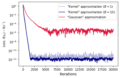
Figure 1: Comparing Algorithm 1 with gradient-free Algorithm from [36] and effect of the parameter $B$ (batch size) on the convergence neighborhood of Zero-Order Mini-batch Stochastic Gradient Descent. Here we optimize $f(x)$ with the parameters: $d=16$ (dimensional of problem), $p=5$ (number of nonlinear equations), $\gamma=0.01$ (smoothing parameter), $\eta\leavevmode\nobreak\ =\leavevmode\nobreak\ 0.01$ (fixed step size), $B=\{1,10\}$ (batch size), $\beta=3$ (order of smoothness).

hello

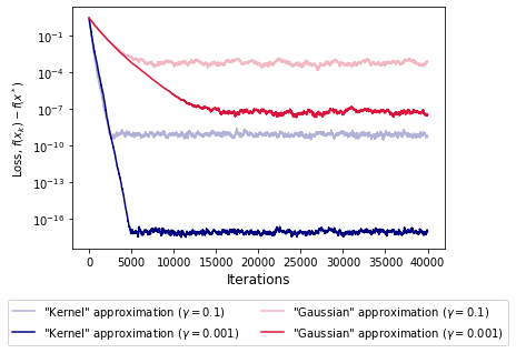
Figure 2: Effect of the parameter $\gamma$ (smoothing parameter) on the error floor. Here we optimize $f(x)$ with parameters: $d=128$ (dimensional of problem), $p\leavevmode\nobreak\ =\leavevmode\nobreak\ 16$ (number of nonlinear equations), $\gamma=\{0.1,0.001\}$ (smoothing parameter), $\eta\leavevmode\nobreak\ =\leavevmode\nobreak\ 0.01$ (fixed step size), $B=2$ (batch size), $\beta=3$ (order of smoothness).

Figure 2 shows the effect of the smoothing parameter $\gamma$ on the error floor. We can observe that the parameter $\gamma$ directly affects the error floor. We also note that with different parameters $\gamma$ the Zero-Order Mini-batch SGD (see Algorithm 1) retains its significant superiority over its counterpart.

To validate the robustness of our Algorithm (1), we now introduce the following gradient approximation via $L_{2}$ randomization which is well considered e.g. in [26]:

$$\tilde{\mathbf{g}}(x,\mathbf{e})=d\frac{f(x+\gamma\mathbf{e})-f(x-\gamma\mathbf{e})}{2\gamma}\mathbf{e},$$ (13)

where $\mathbf{e}$ is uniformly distributed on $S_{2}^{d}(1)$. Then Figure 3 demonstrates the effect of the smoothness order parameter on the convergence rate and the error floor, where "$L_{2}$ approximation" is a gradient-free counterpart of algorithm [36] with (13). We see that $L_{2}$ approximation has the same convergence rate as "Gaussian" approximation, but has a better error floor (i.e. shows efficiency of the randomization). We also observe that the advantages of the high order of smoothness improve the error floor of Algorithm 1. By comparing the $L_{2}$ approximation with Algorithm 1, we see the efficiency of the "Kernel" (in terms of the error floor), which uses information about highly smoothness. See Appendix A for the effect of the parameters $d$ and $p$ on the convergence rate and the error floor.

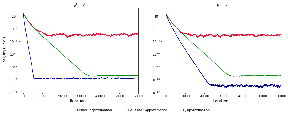
Figure 3: Effect of the parameter $\beta$ on the convergence rate and the error floor. Here we optimize $f(x)$ with the parameters: $d=256$ (dimensional of problem), $p=32$ (number of nonlinear equations), $\gamma=0.1$ (smoothing parameter), $\eta\leavevmode\nobreak\ =\leavevmode\nobreak\ 0.01$ (fixed step size), $B=10$ (batch size), $\beta=\{3,5\}$ (order of smoothness).

9.   Conclusions

We proposed a Zero-Order Minibatch SGD method for solving smooth nonconvex optimization problems under the Polyak–Lojasiewicz condition. We generalized our results to stochastic problems under adversarial noise, considering the possible options: when two-point feedback is available and when only one-point feedback is available. Our algorithm showed efficiency on the standard (for problems under the Polyak–Lojasiewicz condition) example of solving a system of nonlinear equations.

CONFLICT OF INTEREST

The authors declare that they have no conflict if interest.

Appendix A Analyzing effect of problem parameters on algorithms

In Figure 4 we show the effect of the parameters $d$ and $p$ on the convergence rate and error floor. We can observe the behavior of the algorithms via the following approaches of approximating the gradient oracle (see Definition 1): "Kernel" approximation, "Gaussian" approximation and $L_{2}$ approximation at different parameters of the dimensional of the problem and the number of nonlinear equations. When increasing the number of nonlinear equations, we see that all algorithms worsen the convergence rate, but do not change the error floor. And when increasing the dimensional of the problem, we observe that only the "Kernel" approximation and the $L_{2}$ approximation improve the error floor (i.e. shows the efficiency of the randomization). We note that Algorithm 1 surpasses its counterparts in all the above cases (at different parameters), thereby confirming that the Algorithm 1 is robust for solving the problem under the Polyak–Lojasiewicz condition in general.

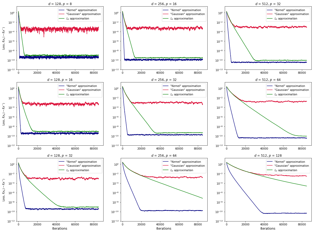
Figure 4: Effect of the parameters $d$ (dimensional of problem) and $p$ (number of nonlinear equations) on the convergence rate and the error floor. Here we optimize $f(x)$ with the following parameters: $d=\{128,256,512\}$ (dimensional of problem), $p=\{8,16,32,64,128\}$ (number of nonlinear equations), $\gamma=0.1$ (smoothing parameter), $\eta\leavevmode\nobreak\ =\leavevmode\nobreak\ 0.01$ (fixed step size), $B=10$ (batch size), $\beta=3$ (order of smoothness).

Appendix B Auxiliary Facts and Results

In this section we list the auxiliary facts and results that we use several times in our proofs.

B.1.   Squared norm of the sum

For all $a_{1},...,a_{n}\in\mathbb{R}^{d}$, where $n=\{2,3\}$

$$\|a_{1}+...+a_{n}\|_{2}^{2}\leq n\|a_{1}\|_{2}^{2}+...+n\|a_{n}\|_{2}^{2}.$$ (14)

B.2.   Fact from concentration of the measure

Let $\mathbf{e}$ is uniformly distributed on the Euclidean unit sphere, then, for $d\geq 8$, $\forall s\in\mathbb{R}^{d}$

$$\mathbb{E}_{\mathbf{e}}\left(\langle s,\mathbf{e}\rangle^{2}\right)\leq\frac{\|s\|_{2}^{2}}{d}.$$ (15)

B.3.   Gaussian smoothing. Upper bounds for the moments

(Proved in Lemma 1, [21]). Let $\mathbf{u}\sim\mathcal{N}(0,1)$ is a random Gaussian vector, then we have

$$\text{for }p\in[0,2] : \mathbb{E}_{u}[\|u\|_{2}^{p}] \leq d^{p/2};$$ (16)

$$\text{for }p\geq 2 : \mathbb{E}_{u}[\|u\|_{2}^{p}] \leq(p+d)^{p/2}.$$ (17)

B.4.   Fact from Gaussian approximation

(Proved in Theorem 3, [21]). Let $f$ is differentiable at $x\in\mathbb{R}^{d}$ and $\mathbf{u}\sim\mathcal{N}(0,1)$ is normally distributed random Gaussian vector, then we have

$$\mathbb{E}_{u}[\langle\nabla f(x),u\rangle^{2}\|u\|_{2}^{2}]\leq(d+4)\|\nabla f(x)\|^{2}_{2}.$$ (18)

B.5.   Taylor expansion

Using the Taylor expansion we have

$$f(x+\gamma re)=f(x)+\langle\nabla f(x),\gamma re\rangle+\sum_{2\leq|n|\leq l}\frac{(r\gamma)^{|n|}}{n!}D^{(n)}f(x)e^{n}+R(\gamma re),$$ (19)

whereby assumption

$$|R(\gamma re)|\leq L\|\gamma re\|_{2}^{\beta}=L|r|^{\beta}\gamma^{\beta}.$$ (20)

B.6.   Kernel property

If $e$ is uniformly distributed on unit sphere we have $\mathbb{E}[ee^{\text{T}}]=(1/d)I_{d\times d}$, where $I_{d\times d}$ is the identity matrix. Therefore, using the facts $\mathbb{E}[rK(r)]=1$ and $\mathbb{E}[r^{|n|}K(r)]=0$ for $2\leq|n|\leq l$ we have

$$\mathbb{E}\left[\frac{d}{\gamma}\left(\langle\nabla f(x),\gamma re\rangle+\sum_{2\leq|n|\leq l}\frac{(r\gamma)^{|n|}}{n!}D^{(n)}f(x)e^{n}\right)K(r)e\right]=\nabla f(x).$$ (21)

B.7.   Bounds of the Weighted Sum of Legendre Polynomials

Let $\kappa_{\beta}=\int|u|^{\beta}|K(u)|du$ and set $\kappa=\int K^{2}(u)du$. Then if $K$ be a weighted sum of Legendre polynomials, then it is proved in (see Appendix A.3, [11]) that $\kappa_{\beta}$ and $\kappa$ do not depend on $d$, they depend only on $\beta$, such that for $\beta\geq 1$:

$$\kappa_{\beta}\leq 2\sqrt{2}(\beta-1),$$ (22)

$$\kappa\leq 3\beta^{3}.$$ (23)

Appendix C The convergence rate of SGD with biased gradient

Lemma 2 (Lemma 1)

Let $\{x_{k}\}_{k\geq 0}$ denote the iterates of Algorithm Mini-batch SGD, function $f$ satisfy Assumptions 1-2 with $\beta=2$, and the gradient oracle (3) satisfy Assumptions 3-4. Then there exists step size $\eta\leavevmode\nobreak\ \leq\leavevmode\nobreak\ \frac{1}{(M+1)L_{2}}$ such that it hold $\forall N\geq 0$ and an arbitrary batch size $B$

$$\mathbb{E}[f(x_{N})]-f^{*}\leq(1-\eta\mu(1-m))^{N}(f(x_{0})-f^{*})+\frac{\zeta^{2}}{2\mu(1-m)}+\frac{\eta L_{2}\sigma^{2}}{2B\mu(1-m)}.$$ (24)

where $L_{2}$ is constant of the Lipschitz gradient such that $\|\nabla f(x)-\nabla f(y)\|_{2}\leq L_{2}\|x-y\|_{2}$.

P r o o f

By the $L_{2}$-smoothness of $f$ and choice of the step size $\eta\leq\frac{1}{(M+1)L_{2}}$ we have

$$\mathbb{E}[f( x_{k+1})]\leq f(x_{k})+\langle\nabla f(x_{k}),x_{k+1}-x_{k}\rangle+\frac{L_{2}}{2}\|x_{k+1}-x_{k}\|_{2}^{2}$$

$$\leq f(x_{k})-\eta\langle\nabla f(x_{k}),\mathbb{E}[\mathbf{g}_{k}]\rangle+\frac{\eta^{2}L_{2}}{2}\left(\mathbb{E}\left[\|\mathbf{g}_{k}-\mathbb{E}[\mathbf{g}_{k}]\|_{2}^{2}\right]+\mathbb{E}\left[\|\mathbb{E}[\mathbf{g}_{k}]\|_{2}^{2}\right]\right)$$

$$\overset{\eqref{eq:Definition_1}}{=}f(x_{k})-\eta\langle\nabla f(x_{k}),\nabla f(x_{k})+\mathbf{b}(x_{k})\rangle+\frac{\eta^{2}L_{2}}{2}\left(\mathbb{E}\left[\|\mathbf{n}(x_{k},\xi)\|_{2}^{2}\right]+\mathbb{E}\left[\|\nabla f(x_{k})+\mathbf{b}(x_{k})\|_{2}^{2}\right]\right)$$

$$\overset{\eqref{eq:Assumption_3}}{\leq}f(x_{k})-\eta\langle\nabla f(x_{k}),\nabla f(x_{k})+\mathbf{b}(x_{k})\rangle+\frac{\eta^{2}L_{2}}{2}\left((M+1)\mathbb{E}\left[\|\nabla f(x_{k})+\mathbf{b}(x_{k})\|_{2}^{2}\right]+\sigma^{2}\right)$$

$$=f(x_{k})+\frac{\eta}{2}\left(\pm\|\nabla f(x_{k})\|^{2}_{2}-2\langle\nabla f(x_{k}),\nabla f(x_{k})+\mathbf{b}(x_{k})\rangle+\|\nabla f(x_{k})+\mathbf{b}(x_{k})\|_{2}^{2}\right)+\frac{\eta^{2}L_{2}}{2}\sigma^{2}$$

$$=f(x_{k})+\frac{\eta}{2}\left(-\|\nabla f(x_{k})\|^{2}_{2}+\|\mathbf{b}(x_{k})\|_{2}^{2}\right)+\frac{\eta^{2}L_{2}}{2}\sigma^{2}$$

$$\overset{\eqref{eq:Assumption_2},\eqref{eq:Assumption_4}}{\leq}(1-\eta\mu(1-m))(f(x_{k})-f^{*})+\frac{\eta\zeta^{2}}{2}+\frac{\eta^{2}L_{2}}{2}\sigma^{2}+f^{*}.$$ (25)

Applying recursion to (25) and adding batching (with batch size $B$) we obtain

$$\mathbb{E}[f(x_{N})]-f^{*}\leq(1-\eta\mu(1-m))^{N}(f(x_{0})-f^{*})+\frac{\zeta^{2}}{2\mu(1-m)}+\frac{\eta L_{2}\sigma^{2}}{2B\mu(1-m)}.$$

Further structure of the appendix has close to block form. In particular, the first block (Appendices D-G) describes in detail the obtaining results for the approach proposed in this article to develop a gradient-free algorithm. Namely, the approach that implied using the "kernel-based" approximation (Kernel approximation) instead of the gradient oracle (3). While the second block (AppendicesH-K) provides a detailed description of obtaining results for the competing approach of developing gradient-free algorithms. In particular, the approach that uses Gaussian approximation instead of the gradient oracle (3). Each block considers different cases of a zero-order oracle. For instance, Appendix D and H consider zero-order oracle with adversarial deterministic noise described in Section 4. The stochastic case with the same concept of adversarial noise in a zero-order oracle generating a gradient approximation with two-point feedback, which is briefly described in the discussion of the results of Theorem 1, is discussed in Appendix E and I. Also in Appendix F and J, the case of a zero-order oracle with adversarial stochastic noise, described in Subsection 5.1, is considered in detail. The final case in each block (Appendix G and K) is a zero-order oracle case, combining adversarial deterministic and stochastic noise considered in Subsection 5.2. Note that the last two considered cases of zero-order oracle generate a gradient approximation with one-point feedback (see Section 5).

Appendix D Proof of Theorem 1

D.1.   Kernel approximation

The "kernel-based" approximation of gradient has the following form (7):

$$\mathbf{\tilde{g}}(x,\mathbf{e})=d\frac{\tilde{f}(x+\gamma r\mathbf{e})-\tilde{f}(x-\gamma r\mathbf{e})}{2\gamma}K(r)\mathbf{e},$$

where $\tilde{f}(x)$ is defined in (6).

D.2.   Bias square

By definition (7) we have

$$\|\mathbb{E}[\mathbf{\tilde{g}}(x, \mathbf{e})]-\nabla f(x)\|_{2}=\|\frac{d}{2\gamma}\mathbb{E}\left[\left(\tilde{f}(x+\gamma r\mathbf{e})-\tilde{f}(x-\gamma r\mathbf{e})\right)\mathbf{e}K(r)\right]-\nabla f(x)\|_{2}$$

$$\overset{\eqref{zero_order_oracle_1}}{=}\phantom{5}\|\frac{d}{2\gamma}\mathbb{E}\left[\left(f(x+\gamma r\mathbf{e})-f(x-\gamma r\mathbf{e})+\delta(x+\gamma r\mathbf{e})-\delta(x-\gamma r\mathbf{e})\right)\mathbf{e}K(r)\right]-\nabla f(x)\|_{2}$$

$$\overset{\eqref{Taylor_expansion_1}}{=}\phantom{5}\|\frac{d}{\gamma}\mathbb{E}[(\langle\nabla f(x),\gamma r\mathbf{e}\rangle+\sum_{2\leq|n|\leq l\;\text{odd}}\frac{(r\gamma)^{|n|}}{n!}D^{(n)}f(x)\mathbf{e}^{n}+\frac{R(\gamma r\mathbf{e})-R(-\gamma r\mathbf{e})}{2}$$

$$\phantom{=\phantom{15}\|\frac{d}{\gamma}\mathbb{E}[(\langle\nabla f(x),\gamma r\mathbf{e}\rangle}\;+\frac{\delta(x+\gamma r\mathbf{e})-\delta(x-\gamma r\mathbf{e})}{2})\mathbf{e}K(r)]-\nabla f(x)\|_{2}$$

$$\overset{\eqref{Kernel_property}}{=}\phantom{5}\|\frac{d}{2\gamma}\mathbb{E}\left[\left(R(\gamma r\mathbf{e})-R(-\gamma r\mathbf{e})+\delta(x+\gamma r\mathbf{e})-\delta(x-\gamma r\mathbf{e})\right)\mathbf{e}K(r)\right]\|_{2}$$

$$\leq\phantom{15}\frac{d}{2\gamma}\mathbb{E}\left[|R(\gamma r\mathbf{e})-R(-\gamma r\mathbf{e})+\delta(x+\gamma r\mathbf{e})-\delta(x-\gamma r\mathbf{e})||K(r)|\right]$$

$$\overset{\eqref{Taylor_expansion_2}}{\leq}\phantom{5}\kappa_{\beta}d\left(L_{\beta}\gamma^{\beta-1}+\frac{\Delta}{\gamma}\right).\qquad/*\mbox{ the distribution of $\mathbf{e}$ is symmetric }*/$$

Then, we can find bias square

$$\|\mathbf{b}(x)\|_{2}^{2}=\|\mathbb{E}[\mathbf{\tilde{g}}(x,\mathbf{e})]-\nabla f(x)\|_{2}^{2}\overset{\eqref{Squared_norm_of_the_sum}}{\leq}2\kappa_{\beta}^{2}d^{2}L_{\beta}^{2}\gamma^{2(\beta-1)}+2\frac{\kappa_{\beta}^{2}d^{2}\Delta^{2}}{\gamma^{2}}.$$ (26)

D.3.   Second moment

By definition (7) we have

$$\mathbb{E}\left[\|\mathbf{\tilde{g}}(x,e)\|^{2}_{2}\right] = \frac{d^{2}}{4\gamma^{2}}\mathbb{E}\left[\|\left(f(x+\gamma re)-f(x-\gamma re)+\delta(x+\gamma re)-\delta(x-\gamma re)\right)K(r)e\|^{2}_{2}\right]$$ (27)

$$= \frac{d^{2}}{4\gamma^{2}}\mathbb{E}\left[\left(f(x+\gamma re)-f(x-\gamma re)+2\delta(x+\gamma re)\right)^{2}K^{2}(r)\|e\|_{2}^{2}\right]$$

$$\overset{\eqref{Squared_norm_of_the_sum}}{\leq} \frac{d^{2}}{2\gamma^{2}}\left(\mathbb{E}\left[\left(f(x+\gamma re)-f(x-\gamma re)\right)^{2}K^{2}(r)\right]+4\kappa\Delta^{2}\right).$$

Using fact $\sqrt{\mathbb{E}\left[\|e\|_{q}^{4}\right]}\leq\min\left\{q-1,16\ln d-8\right\}d^{2/q-1}$ to the first multiplier (27) we get

$$\frac{d^{2}}{2\gamma^{2}}\mathbb{E}_{e}[(f(x+\gamma re) -f(x-\gamma re))^{2}]=\frac{d^{2}}{2\gamma^{2}}\mathbb{E}_{e}\left[\left((f(x+\gamma re)-f(x-\gamma re)\pm f(x)\pm 2\langle\nabla f(x),\gamma re\rangle\right)^{2}\right]$$

$$\overset{\eqref{Squared_norm_of_the_sum}}{\leq}\phantom{5}\frac{3d^{2}}{2\gamma^{2}}\mathbb{E}_{e}\left[(f(x+\gamma re)-f(x)-\langle\nabla f(x),\gamma re\rangle\right)^{2}$$

$$\phantom{\leq\phantom{5}\frac{3d^{2}}{2\gamma^{2}}\mathbb{E}}+\left(f(x-\gamma re)-f(x)-\langle\nabla f(x),-\gamma re\rangle)^{2}+4\langle\nabla f(x),\gamma re\rangle^{2}\right]$$

$$\leq\phantom{15}\frac{3d^{2}}{2\gamma^{2}}\mathbb{E}_{e}\left[\frac{L_{2}^{2}}{2}\|\gamma re\|_{2}^{4}+4\langle\nabla f(x),\gamma re\rangle^{2}\right]$$ (28)

$$\overset{\eqref{Concentration_measure}}{\leq}\phantom{5}\frac{3d^{2}}{2\gamma^{2}}\left(\frac{L_{2}^{2}\gamma^{4}}{2}\mathbb{E}_{e}\left[\|e\|_{2}^{4}\right]+\frac{4\gamma^{2}\|\nabla f(x)\|_{2}^{2}}{d}\right)$$

$$\leq\phantom{15}6d\|\nabla f(x)\|_{2}^{2}+\frac{3d^{2}L_{2}^{2}\gamma^{2}}{4},$$ (29)

where (28) we obtained by applying the property of the Lipschitz continuous gradient.

By substituting (29) into (27) and using independence of $e$ and $r$ we obtain

$$\mathbb{E}\left[\|\mathbf{\tilde{g}}(x,e)\|_{2}^{2}\right]\leq\kappa\left(6d\|\nabla f(x)\|_{2}^{2}+\frac{3d^{2}L_{2}^{2}\gamma^{2}}{4}+\frac{2d^{2}\Delta^{2}}{\gamma^{2}}\right).$$ (30)

D.4.   Convergence rate

From the inequalities (26) and (30) we can conclude that Assumption 3 holds with the choice

$$\sigma^{2}\overset{\eqref{eq_remark_2}}{=}\mathcal{O}\left(\beta^{3}d^{2}L_{2}^{2}\gamma^{2}+\frac{\beta^{3}d^{2}\Delta^{2}}{\gamma^{2}}\right),\;\;\;M=\mathcal{O}\left(\beta^{3}d\right).$$ (31)

and that Assumption 4 also holds with the choice

$$m=0,\zeta^{2}\overset{\eqref{eq_remark_1}}{=}\mathcal{O}\left(\beta^{2}d^{2}L_{\beta}^{2}\gamma^{2(\beta-1)}+\frac{\beta^{2}d^{2}\Delta^{2}}{\gamma^{2}}\right).$$ (32)

Now to find the asymptote to which the Algorithm 1 converges with the gradient approximation (7), substitute the parameters (31), (32) into the second and third terms (24) with $\eta=\mathcal{O}\left(1/M\right)$:

$$\mathbb{E}[f(x_{N})]-f^{*}\leq\frac{\zeta^{2}}{2\mu(1-m)}+\frac{\eta L_{2}\sigma^{2}}{2B\mu(1-m)}=\mathcal{O}\left(\beta^{2}d^{2}L_{\beta}^{2}\gamma^{2(\beta-1)}+\frac{\beta^{2}d^{2}\Delta^{2}}{\gamma^{2}}+\frac{dL_{2}^{2}\gamma^{2}}{B}+\frac{d\Delta^{2}}{B\gamma^{2}}\right).$$

Since $B$ can be taken as large, the first two terms are responsible for the asymptote. We find the optimal smoothing parameter $\gamma$ that minimizes the first two terms:

$$\mathbb{E}[f(x_{N})]-f^{*}\leq\beta^{2}d^{2}\gamma^{2(\beta-1)}+\frac{\beta^{2}d^{2}\Delta^{2}}{\gamma^{2}}=\mathcal{O}\left(d^{2}\Delta^{\frac{2(\beta-1)}{\beta}}\right),$$ (33)

where $\gamma=\Delta^{1/\beta}$ is optimal smoothing parameter. Then from (33) we can find the maximum noise level, assuming that $d^{2}\Delta\leq\varepsilon$, for $\varepsilon>0$ then we have

$$\Delta=\mathcal{O}\left(\varepsilon^{\frac{\beta}{2(\beta-1)}}d^{\frac{-\beta}{\beta-1}}\right).$$

Appendix E Proof of convergence of Algorithm 1 with two-point feedback

E.1.   Kernel approximation

The "kernel-based" approximation of gradient has the following form:

$$\mathbf{\tilde{g}}(x,\xi,\mathbf{e})=d\frac{\tilde{f}(x+\gamma r\mathbf{e},\xi)-\tilde{f}(x-\gamma r\mathbf{e},\xi)}{2\gamma}K(r)\mathbf{e},$$ (34)

where the zero-order oracle $\tilde{f}(x,\xi)$ is defined as follows:

$$\tilde{f}(x,\xi)=f(x,\xi)+\delta(x),$$ (35)

$\delta(x)$ is adversarial deterministic noise, $|\delta(x)|\leq\Delta$ is a level of noise.

E.2.   Bias square

By definition (34) we have

$$\|\mathbb{E}[\mathbf{\tilde{g}}(x, \xi,\mathbf{e})]-\nabla f(x)\|_{2}=\|\frac{d}{2\gamma}\mathbb{E}\left[\left(\tilde{f}(x+\gamma r\mathbf{e},\xi)-\tilde{f}(x-\gamma r\mathbf{e},\xi)\right)\mathbf{e}K(r)\right]-\nabla f(x)\|_{2}$$

$$\overset{\eqref{Stochastic_Problem},\eqref{zero_order_oracle_2}}{=}\|\frac{d}{2\gamma}\mathbb{E}\left[\left(f(x+\gamma r\mathbf{e})-f(x-\gamma r\mathbf{e})+\delta(x+\gamma r\mathbf{e})-\delta(x-\gamma r\mathbf{e})\right)\mathbf{e}K(r)\right]-\nabla f(x)\|_{2}$$

$$\overset{\eqref{Taylor_expansion_1}}{=}\phantom{88}\|\frac{d}{\gamma}\mathbb{E}[(\langle\nabla f(x),\gamma r\mathbf{e}\rangle+\sum_{2\leq|n|\leq l\;\text{odd}}\frac{(r\gamma)^{|n|}}{n!}D^{(n)}f(x)\mathbf{e}^{n}+\frac{R(\gamma r\mathbf{e})-R(-\gamma r\mathbf{e})}{2}$$

$$\phantom{\overset{\eqref{Taylor_expansion_1}}{=}\phantom{88}\|\frac{d}{\gamma}\mathbb{E}[(\langle\nabla f(x),\gamma r\mathbf{e}\rangle}\;+\frac{\delta(x+\gamma r\mathbf{e})-\delta(x-\gamma r\mathbf{e})}{2})\mathbf{e}K(r)]-\nabla f(x)\|_{2}$$

$$\overset{\eqref{Kernel_property}}{=}\phantom{88}\|\frac{d}{2\gamma}\mathbb{E}\left[\left(R(\gamma r\mathbf{e})-R(-\gamma r\mathbf{e})+\delta(x+\gamma r\mathbf{e})-\delta(x-\gamma r\mathbf{e})\right)\mathbf{e}K(r)\right]\|_{2}$$

$$\leq\phantom{888}\frac{d}{2\gamma}\mathbb{E}\left[|R(\gamma r\mathbf{e})-R(-\gamma r\mathbf{e})+\delta(x+\gamma r\mathbf{e})-\delta(x-\gamma r\mathbf{e})||K(r)|\right]$$

$$\overset{\eqref{Taylor_expansion_2}}{\leq}\phantom{88}\kappa_{\beta}d\left(L_{\beta}\gamma^{\beta-1}+\frac{\Delta}{\gamma}\right).\qquad/*\mbox{ the distribution of $\mathbf{e}$ is symmetric }*/$$

Then, we can find bias square

$$\|\mathbf{b}(x)\|_{2}^{2}=\|\mathbb{E}[\mathbf{\tilde{g}}(x,\xi,\mathbf{e})]-\nabla f(x)\|_{2}^{2}\leq\left(\kappa_{\beta}dL_{\beta}\gamma^{\beta-1}+\frac{\kappa_{\beta}d\Delta}{\gamma}\right)^{2}\overset{\eqref{Squared_norm_of_the_sum}}{\leq}\frac{2\kappa_{\beta}^{2}d^{2}}{\gamma^{2}}\left(L_{\beta}^{2}\gamma^{2\beta}+\Delta^{2}\right).$$ (36)

E.3.   Second moment

By definition (34) we have

$$\mathbb{E}\left[\|\mathbf{\tilde{g}}(x,\xi,e)\|^{2}_{2}\right] =\phantom{88}\frac{d^{2}}{4\gamma^{2}}\mathbb{E}\left[\|\left(f(x+\gamma re,\xi)-f(x-\gamma re,\xi)+\delta(x+\gamma re)-\delta(x-\gamma re)\right)K(r)e\|^{2}_{2}\right]$$

$$=\phantom{88}\frac{d^{2}}{4\gamma^{2}}\mathbb{E}\left[\left(f(x+\gamma re,\xi)-f(x-\gamma re,\xi)+2\delta(x+\gamma re)\right)^{2}K^{2}(r)\|e\|_{2}^{2}\right]$$

$$\overset{\eqref{Squared_norm_of_the_sum}}{\leq}\phantom{8}\frac{d^{2}}{2\gamma^{2}}\left(\mathbb{E}\left[\left(f(x+\gamma re,\xi)-f(x-\gamma re,\xi)\right)^{2}K^{2}(r)\right]+4\kappa\Delta^{2}\right).$$ (37)

Using fact $\sqrt{\mathbb{E}\left[\|e\|_{q}^{4}\right]}\leq\min\left\{q-1,16\ln d-8\right\}d^{2/q-1}$ to the first multiplier (37) we get

$$\frac{d^{2}}{2\gamma^{2}}\mathbb{E}_{e}[(f(x +\gamma re,\xi)-f(x-\gamma re,\xi))^{2}]$$

$$=\phantom{88}\frac{d^{2}}{2\gamma^{2}}\mathbb{E}_{e}\left[\left((f(x+\gamma re,\xi)-f(x-\gamma re,\xi)\pm f(x,\xi)\pm 2\langle\nabla f(x,\xi),\gamma re\rangle\right)^{2}\right]$$

$$\overset{\eqref{Squared_norm_of_the_sum}}{\leq}\phantom{8}\frac{3d^{2}}{2\gamma^{2}}\mathbb{E}_{e}\left[(f(x+\gamma re,\xi)-f(x,\xi)-\langle\nabla f(x,\xi),\gamma re\rangle\right)^{2}$$

$$\phantom{\overset{\eqref{Squared_norm_of_the_sum}}{\leq}\frac{3d^{2}}{2\gamma^{2}}\mathbb{E}_{e}}+\left(f(x-\gamma re,\xi)-f(x,\xi)-\langle\nabla f(x,\xi),-\gamma re\rangle)^{2}+4\langle\nabla f(x,\xi),\gamma re\rangle^{2}\right]$$

$$\leq\phantom{88}\frac{3d^{2}}{2\gamma^{2}}\mathbb{E}_{e}\left[\frac{L_{2}^{2}}{2}\|\gamma re\|_{2}^{4}+4\langle\nabla f(x,\xi),\gamma re\rangle^{2}\right]$$ (38)

$$\overset{\eqref{Concentration_measure}}{\leq}\phantom{8}\frac{3d^{2}}{2\gamma^{2}}\left(\frac{L_{2}^{2}\gamma^{4}}{2}\mathbb{E}_{e}\left[\|e\|_{2}^{4}\right]+\frac{4\gamma^{2}\|\nabla f(x,\xi)\|_{2}^{2}}{d}\right)$$

$$\leq\phantom{88}6d\|\nabla f(x,\xi)\|_{2}^{2}+\frac{3d^{2}L_{2}^{2}\gamma^{2}}{4},$$ (39)

where (38) we obtained by applying the property of the Lipschitz continuous gradient.

By substituting (39) into (37) and using independence of $e$ and $r$ we obtain

$$\mathbb{E}\left[\|\mathbf{\tilde{g}}(x,\xi,e)\|_{2}^{2}\right]\leq\kappa\left(6d\|\nabla f(x,\xi)\|_{2}^{2}+\frac{3d^{2}L_{2}^{2}\gamma^{2}}{4}+\frac{2d^{2}\Delta^{2}}{\gamma^{2}}\right).$$ (40)

E.4.   Convergence rate

From the inequalities (36) and (40) we can conclude that Assumption 3 holds with the choice

$$\sigma^{2}\overset{\eqref{eq_remark_2}}{=}\mathcal{O}\left(\beta^{3}d^{2}L_{2}^{2}\gamma^{2}+\frac{\beta^{3}d^{2}\Delta^{2}}{\gamma^{2}}\right),\;\;\;M=\mathcal{O}\left(\beta^{3}d\right).$$ (41)

and that Assumption 4 also holds with the choice

$$m=0,\zeta^{2}\overset{\eqref{eq_remark_1}}{=}\mathcal{O}\left(\beta^{2}d^{2}L_{\beta}^{2}\gamma^{2(\beta-1)}+\frac{\beta^{2}d^{2}\Delta^{2}}{\gamma^{2}}\right).$$ (42)

Now to find the asymptote to which the Algorithm 1 converges with the gradient approximation (34), substitute the parameters (41), (42) into the second and third terms (24) with $\eta=\mathcal{O}\left(1/M\right)$:

$$\mathbb{E}[f(x_{N})]-f^{*}\leq\frac{\zeta^{2}}{2\mu(1-m)}+\frac{\eta L_{2}\sigma^{2}}{2B\mu(1-m)}=\mathcal{O}\left(\beta^{2}d^{2}L_{\beta}^{2}\gamma^{2(\beta-1)}+\frac{\beta^{2}d^{2}\Delta^{2}}{\gamma^{2}}+\frac{dL_{2}^{2}\gamma^{2}}{B}+\frac{d\Delta^{2}}{B\gamma^{2}}\right).$$

Since $B$ can be taken as large, the first two terms are responsible for the asymptote. We find the optimal smoothing parameter $\gamma$ that minimizes the first two terms:

$$\mathbb{E}[f(x_{N})]-f^{*}\leq\beta^{2}d^{2}\gamma^{2(\beta-1)}+\frac{\beta^{2}d^{2}\Delta^{2}}{\gamma^{2}}=\mathcal{O}\left(d^{2}\Delta^{\frac{2(\beta-1)}{\beta}}\right),$$ (43)

where $\gamma=\Delta^{1/\beta}$ is optimal smoothing parameter. Then from (43) we can find the maximum noise level, assuming that $d^{2}\Delta\leq\varepsilon$, for $\varepsilon>0$ then we have

$$\Delta=\mathcal{O}\left(\varepsilon^{\frac{\beta}{2(\beta-1)}}d^{\frac{-\beta}{\beta-1}}\right).$$

Appendix F Proof of Theorem 2

F.1.   Kernel approximation

The "kernel-based" approximation of gradient has the following form (9):

$$\mathbf{\tilde{g}}(x,\xi,\mathbf{e})=d\frac{\tilde{f}(x+\gamma r\mathbf{e},\xi_{1})-\tilde{f}(x-\gamma r\mathbf{e},\xi_{2})}{2\gamma}K(r)\mathbf{e},$$

where $\tilde{f}(x,\xi)$ is defined in (10).

F.2.   Bias square

By definition (9) we have

$$\|\mathbb{E}[\mathbf{\tilde{g}}(x,\xi,\mathbf{e})]-\nabla f(x)\|_{2}\phantom{88} =\phantom{88}\|\frac{d}{2\gamma}\mathbb{E}\left[\left(\tilde{f}(x+\gamma r\mathbf{e},\xi)-\tilde{f}(x-\gamma r\mathbf{e},\xi)\right)\mathbf{e}K(r)\right]-\nabla f(x)\|_{2}$$

$$\overset{\eqref{zero_order_oracle_3}}{=}\phantom{8}\,\|\frac{d}{2\gamma}\mathbb{E}\left[\left(f(x+\gamma r\mathbf{e})-f(x-\gamma r\mathbf{e})+\xi_{1}-\xi_{2}\right)\mathbf{e}K(r)\right]-\nabla f(x)\|_{2}$$

$$\overset{\eqref{Taylor_expansion_1}}{=}\phantom{8}\,\|\frac{d}{\gamma}\mathbb{E}[(\langle\nabla f(x),\gamma r\mathbf{e}\rangle+\sum_{2\leq|n|\leq l\;\text{odd}}\frac{(r\gamma)^{|n|}}{n!}D^{(n)}f(x)\mathbf{e}^{n}$$

$$\phantom{\overset{\eqref{Taylor_expansion_1}}{=}\phantom{8}\,\|\frac{d}{\gamma}\mathbb{E}[(\langle\nabla f(x),\gamma r\mathbf{e}\rangle}\;+\frac{R(\gamma r\mathbf{e})-R(-\gamma r\mathbf{e})}{2})\mathbf{e}K(r)]-\nabla f(x)\|_{2}$$

$$\overset{\eqref{Kernel_property}}{=}\phantom{8}\;\|\frac{d}{2\gamma}\mathbb{E}\left[\left(R(\gamma r\mathbf{e})-R(-\gamma r\mathbf{e})\right)\mathbf{e}K(r)\right]\|_{2}$$

$$\leq\phantom{88}\frac{d}{2\gamma}\mathbb{E}\left[|R(\gamma r\mathbf{e})-R(-\gamma r\mathbf{e})||K(r)|\right]$$

$$\overset{\eqref{Taylor_expansion_2}}{\leq}\phantom{8}\;\kappa_{\beta}dL_{\beta}\gamma^{\beta-1}.$$

Then, we can find bias square

$$\|\mathbf{b}(x)\|_{2}^{2}=\|\mathbb{E}[\mathbf{\tilde{g}}(x,\xi,\mathbf{e})]-\nabla f(x)\|_{2}^{2}\leq\left(\kappa_{\beta}dL_{\beta}\gamma^{\beta-1}\right)^{2}=\kappa_{\beta}^{2}d^{2}L_{\beta}^{2}\gamma^{2(\beta-1)}.$$ (44)

F.3.   Second moment

By definition (9) we have

$$\mathbb{E}\left[\|\mathbf{\tilde{g}}(x,\xi,e)\|^{2}_{2}\right] = \frac{d^{2}}{4\gamma^{2}}\mathbb{E}\left[\|\left(f(x+\gamma re)-f(x-\gamma re)+\xi_{1}-\xi_{2}\right)K(r)e\|^{2}_{2}\right]$$ (45)

$$= \frac{d^{2}}{4\gamma^{2}}\mathbb{E}\left[\left(f(x+\gamma re)-f(x-\gamma re)+\xi_{1}-\xi_{2}\right)^{2}K^{2}(r)\|e\|_{2}^{2}\right]$$

$$\overset{\eqref{Squared_norm_of_the_sum}}{\leq} \frac{d^{2}}{2\gamma^{2}}\left(\mathbb{E}\left[\left(f(x+\gamma re)-f(x-\gamma re)\right)^{2}K^{2}(r)\right]+4\kappa\tilde{\Delta}^{2}\right).$$

Using fact $\sqrt{\mathbb{E}\left[\|e\|_{q}^{4}\right]}\leq\min\left\{q-1,16\ln d-8\right\}d^{2/q-1}$ to the first multiplier (37) we get

$$\frac{d^{2}}{2\gamma^{2}}\mathbb{E}_{e} \left[\left(f(x+\gamma re)-f(x-\gamma re)\right)^{2}\right]$$

$$=\phantom{88}\frac{d^{2}}{2\gamma^{2}}\mathbb{E}_{e}\left[\left((f(x+\gamma re)-f(x-\gamma re)\pm f(x)\pm 2\langle\nabla f(x),\gamma re\rangle\right)^{2}\right]$$

$$\overset{\eqref{Squared_norm_of_the_sum}}{\leq}\phantom{8}\frac{3d^{2}}{2\gamma^{2}}\mathbb{E}_{e}\left[(f(x+\gamma re)-f(x)-\langle\nabla f(x),\gamma re\rangle\right)^{2}$$

$$\phantom{\overset{\eqref{Squared_norm_of_the_sum}}{\leq}\,\frac{3d^{2}}{2\gamma^{2}}\mathbb{E}_{e}}+\left(f(x-\gamma re)-f(x)-\langle\nabla f(x),-\gamma re\rangle)^{2}+4\langle\nabla f(x),\gamma re\rangle^{2}\right]$$

$$\leq\phantom{88}\frac{3d^{2}}{2\gamma^{2}}\mathbb{E}_{e}\left[\frac{L_{2}^{2}}{2}\|\gamma re\|_{2}^{4}+4\langle\nabla f(x),\gamma re\rangle^{2}\right]$$ (46)

$$\overset{\eqref{Concentration_measure}}{\leq}\phantom{8}\frac{3d^{2}}{2\gamma^{2}}\left(\frac{L_{2}^{2}\gamma^{4}}{2}\mathbb{E}_{e}\left[\|e\|_{2}^{4}\right]+\frac{4\gamma^{2}\|\nabla f(x)\|_{2}^{2}}{d}\right)$$

$$\leq\phantom{88}6d\|\nabla f(x)\|_{2}^{2}+\frac{3d^{2}L_{2}^{2}\gamma^{2}}{4},$$ (47)

where (46) we obtained by applying the property of the Lipschitz continuous gradient.

By substituting (47) into (45) and using independence of $e$ and $r$ we obtain

$$\mathbb{E}\left[\|\mathbf{\tilde{g}}(x,\xi,e)\|_{2}^{2}\right]\leq\kappa\left(6d\|\nabla f(x)\|_{2}^{2}+\frac{3d^{2}L_{2}^{2}\gamma^{2}}{4}+\frac{2d^{2}\tilde{\Delta^{2}}}{\gamma^{2}}\right).$$ (48)

F.4.   Convergence rate

From the inequalities (44) and (48) we can conclude that Assumption 3 holds with the choice

$$\sigma^{2}\overset{\eqref{eq_remark_2}}{=}\mathcal{O}\left(\beta^{3}d^{2}L_{2}^{2}\gamma^{2}+\frac{\beta^{3}d^{2}\tilde{\Delta}^{2}}{\gamma^{2}}\right),\;\;\;M=\mathcal{O}\left(\beta^{3}d\right).$$ (49)

and that Assumption 4 also holds with the choice

$$m=0,\zeta^{2}\overset{\eqref{eq_remark_1}}{=}\mathcal{O}\left(\beta^{2}d^{2}L_{\beta}^{2}\gamma^{2(\beta-1)}\right).$$ (50)

Now to find the asymptote to which the Algorithm 1 converges with the gradient approximation (9), substitute the parameters (49), (50) into the second and third terms (24) with $\eta=\mathcal{O}\left(1/M\right)$:

$$\mathbb{E}[f(x_{N})]-f^{*}\leq\frac{\zeta^{2}}{2\mu(1-m)}+\frac{\eta L_{2}\sigma^{2}}{2B\mu(1-m)}=\mathcal{O}\left(\beta^{2}d^{2}L_{\beta}^{2}\gamma^{2(\beta-1)}+\frac{dL_{2}^{2}\gamma^{2}}{B}+\frac{d\tilde{\Delta}^{2}}{B\gamma^{2}}\right).$$

Since the batch size $B$ can be taken large enough, there are no restrictions on the smoothing parameter $\gamma$. Therefore, using the concept of the zero-order oracle (10) Zero-order Mini-batch SGD (see Algorithm 1) with gradient approximation (9) can achieve the desired accuracy.

Appendix G Proof of Theorem 3

G.1.   Kernel approximation

The "kernel-based" approximation of gradient has the following form (11):

$$\mathbf{\tilde{g}}(x,\xi,\mathbf{e})=d\frac{\tilde{f}(x+\gamma r\mathbf{e},\xi_{1})-\tilde{f}(x-\gamma r\mathbf{e},\xi_{2})}{2\gamma}K(r)\mathbf{e},$$

where $\tilde{f}(x,\xi)$ is defined in (12).

G.2.   Bias square

By definition (11) we have

$$\|\mathbb{E}[\mathbf{\tilde{g}}(x, \xi,\mathbf{e})]-\nabla f(x)\|_{2}=\|\frac{d}{2\gamma}\mathbb{E}\left[\left(\tilde{f}(x+\gamma r\mathbf{e},\xi_{1})-\tilde{f}(x-\gamma r\mathbf{e},\xi_{2})\right)\mathbf{e}K(r)\right]-\nabla f(x)\|_{2}$$

$$\overset{\eqref{Stochastic_Problem},\eqref{zero_order_oracle_4}}{=}\|\frac{d}{2\gamma}\mathbb{E}\left[\left(f(x+\gamma r\mathbf{e})-f(x-\gamma r\mathbf{e})+\delta(x+\gamma r\mathbf{e})-\delta(x-\gamma r\mathbf{e})\right)\mathbf{e}K(r)\right]-\nabla f(x)\|_{2}$$

$$\overset{\eqref{Taylor_expansion_1}}{=}\phantom{88}\,\|\frac{d}{\gamma}\mathbb{E}[(\langle\nabla f(x),\gamma r\mathbf{e}\rangle+\sum_{2\leq|n|\leq l\;\text{odd}}\frac{(r\gamma)^{|n|}}{n!}D^{(n)}f(x)\mathbf{e}^{n}+\frac{R(\gamma r\mathbf{e})-R(-\gamma r\mathbf{e})}{2}$$

$$\phantom{\overset{\eqref{Taylor_expansion_1}}{=}\phantom{88}\,\|\frac{d}{\gamma}\mathbb{E}[(\langle\nabla f(x),\gamma r\mathbf{e}\rangle}\;+\frac{\delta(x+\gamma r\mathbf{e})-\delta(x-\gamma r\mathbf{e})}{2})\mathbf{e}K(r)]-\nabla f(x)\|_{2}$$

$$\overset{\eqref{Kernel_property}}{=}\phantom{88}\,\|\frac{d}{2\gamma}\mathbb{E}\left[\left(R(\gamma r\mathbf{e})-R(-\gamma r\mathbf{e})+\delta(x+\gamma r\mathbf{e})-\delta(x-\gamma r\mathbf{e})\right)\mathbf{e}K(r)\right]\|_{2}$$

$$\leq\phantom{888}\frac{d}{2\gamma}\mathbb{E}\left[|R(\gamma r\mathbf{e})-R(-\gamma r\mathbf{e})+\delta(x+\gamma r\mathbf{e})-\delta(x-\gamma r\mathbf{e})||K(r)|\right]$$

$$\overset{\eqref{Taylor_expansion_2}}{\leq}\phantom{88}\;\kappa_{\beta}d\left(L_{\beta}\gamma^{\beta-1}+\frac{\Delta}{\gamma}\right).\qquad/*\mbox{ the distribution of $\mathbf{e}$ is symmetric }*/$$

Then, we can find bias square

$$\|\mathbf{b}(x)\|_{2}^{2}=\|\mathbb{E}[\mathbf{\tilde{g}}(x,\xi,\mathbf{e})]-\nabla f(x)\|_{2}^{2}\overset{\eqref{Squared_norm_of_the_sum}}{\leq}2\kappa_{\beta}^{2}d^{2}L_{\beta}^{2}\gamma^{2(\beta-1)}+2\frac{\kappa_{\beta}^{2}d^{2}\Delta^{2}}{\gamma^{2}}.$$ (51)

G.3.   Second moment

By definition (11) we have

$$\mathbb{E}\left[\|\mathbf{\tilde{g}}(x,\xi,e)\|^{2}_{2}\right] =\frac{d^{2}}{4\gamma^{2}}\mathbb{E}\left[\|\left(f(x+\gamma re)-f(x-\gamma re)+\delta(x+\gamma r\mathbf{e})-\delta(x-\gamma re)+\xi_{1}-\xi_{2}\right)K(r)e\|^{2}_{2}\right]$$

$$=\frac{d^{2}}{4\gamma^{2}}\mathbb{E}\left[\left(f(x+\gamma re)-f(x-\gamma re)+2\delta(x+\gamma re)+\xi_{1}-\xi_{2}\right)^{2}K^{2}(r)\|e\|_{2}^{2}\right]$$

$$\overset{\eqref{Squared_norm_of_the_sum}}{\leq}\frac{d^{2}}{2\gamma^{2}}\left(\mathbb{E}\left[\left(f(x+\gamma re)-f(x-\gamma re)\right)^{2}K^{2}(r)\right]+4\kappa\Delta^{2}+4\kappa\tilde{\Delta}^{2}\right).$$ (52)

Using fact $\sqrt{\mathbb{E}\left[\|e\|_{q}^{4}\right]}\leq\min\left\{q-1,16\ln d-8\right\}d^{2/q-1}$ to the first multiplier (52) we get

$$\frac{d^{2}}{2\gamma^{2}}\mathbb{E}_{e}[(f(x +\gamma re)-f(x-\gamma re))^{2}]$$

$$=\phantom{88}\frac{d^{2}}{2\gamma^{2}}\mathbb{E}_{e}\left[\left((f(x+\gamma re)-f(x-\gamma re)\pm f(x)\pm 2\langle\nabla f(x),\gamma re\rangle\right)^{2}\right]$$

$$\overset{\eqref{Squared_norm_of_the_sum}}{\leq}\phantom{8}\frac{3d^{2}}{2\gamma^{2}}\mathbb{E}_{e}\left[(f(x+\gamma re)-f(x)-\langle\nabla f(x),\gamma re\rangle\right)^{2}$$

$$\phantom{\leq\phantom{8}\frac{3d^{2}}{2\gamma^{2}}\mathbb{E}}+\left(f(x-\gamma re)-f(x)-\langle\nabla f(x),-\gamma re\rangle)^{2}+4\langle\nabla f(x),\gamma re\rangle^{2}\right]$$

$$\leq\phantom{88}\frac{3d^{2}}{2\gamma^{2}}\mathbb{E}_{e}\left[\frac{L_{2}^{2}}{2}\|\gamma re\|_{2}^{4}+4\langle\nabla f(x),\gamma re\rangle^{2}\right]$$ (53)

$$\overset{\eqref{Concentration_measure}}{\leq}\phantom{8}\frac{3d^{2}}{2\gamma^{2}}\left(\frac{L_{2}^{2}\gamma^{4}}{2}\mathbb{E}_{e}\left[\|e\|_{2}^{4}\right]+\frac{4\gamma^{2}\|\nabla f(x)\|_{2}^{2}}{d}\right)$$

$$\leq\phantom{88}6d\|\nabla f(x)\|_{2}^{2}+\frac{3d^{2}L_{2}^{2}\gamma^{2}}{4},$$ (54)

where (53) we obtained by applying the property of the Lipschitz continuous gradient.

By substituting (54) into (52) and using independence of $e$ and $r$ we obtain

$$\mathbb{E}\left[\|\mathbf{\tilde{g}}(x,\xi,e)\|_{2}^{2}\right]\leq\kappa\left(6d\|\nabla f(x,\xi)\|_{2}^{2}+\frac{3d^{2}L_{2}^{2}\gamma^{2}}{4}+\frac{2d^{2}(\Delta^{2}+\tilde{\Delta}^{2})}{\gamma^{2}}\right).$$ (55)

G.4.   Convergence rate

From the inequalities (51) and (55) we can conclude that Assumption 3 holds with the choice

$$\sigma^{2}\overset{\eqref{eq_remark_2}}{=}\mathcal{O}\left(\beta^{3}d^{2}L_{2}^{2}\gamma^{2}+\frac{\beta^{3}d^{2}(\Delta^{2}+\tilde{\Delta}^{2})}{\gamma^{2}}\right),\;\;\;M=\mathcal{O}\left(\beta^{3}d\right).$$ (56)

and that Assumption 4 also holds with the choice

$$m=0,\zeta^{2}\overset{\eqref{eq_remark_1}}{=}\mathcal{O}\left(\beta^{2}d^{2}L_{\beta}^{2}\gamma^{2(\beta-1)}+\frac{\beta^{2}d^{2}\Delta^{2}}{\gamma^{2}}\right).$$ (57)

Now to find the asymptote to which the Algorithm 1 converges with the gradient approximation (11), substitute the parameters (56), (57) into the second and third terms (24) with $\eta=\mathcal{O}\left(1/M\right)$:

$$\mathbb{E}[f(x_{N})]-f^{*}\leq\frac{\zeta^{2}}{2\mu(1-m)}+\frac{\eta L_{2}\sigma^{2}}{2B\mu(1-m)}=\mathcal{O}\left(\beta^{2}d^{2}L_{\beta}^{2}\gamma^{2(\beta-1)}+\frac{\beta^{2}d^{2}\Delta^{2}}{\gamma^{2}}+\frac{dL_{2}^{2}\gamma^{2}}{B}+\frac{d(\Delta^{2}+\tilde{\Delta}^{2})}{B\gamma^{2}}\right).$$

Since $B$ can be taken as large, the first two terms are responsible for the asymptote. We find the optimal smoothing parameter $\gamma$ that minimizes the first two terms:

$$\mathbb{E}[f(x_{N})]-f^{*}\leq\beta^{2}d^{2}\gamma^{2(\beta-1)}+\frac{\beta^{2}d^{2}\Delta^{2}}{\gamma^{2}}=\mathcal{O}\left(d^{2}\Delta^{\frac{2(\beta-1)}{\beta}}\right),$$ (58)

where $\gamma=\Delta^{1/\beta}$ is optimal smoothing parameter. Then from (58) we can find the maximum noise level, assuming that $d^{2}\Delta\leq\varepsilon$, for $\varepsilon>0$ then we have

$$\Delta=\mathcal{O}\left(\varepsilon^{\frac{\beta}{2(\beta-1)}}d^{\frac{-\beta}{\beta-1}}\right).$$

Appendix H Gaussian smoothing approach for Theorem 1

H.1.   Definition Gaussian approximation

Let $\mathbf{u}\sim\mathcal{N}(0,1)$ is a random Gaussian vector, $\gamma>0$ is smoothing parameter then Gaussian smoothing approximation has the following form:

$$\tilde{\mathbf{g}}(x,\mathbf{u})=\frac{\tilde{f}(x+\gamma\mathbf{u})-\tilde{f}(x)}{\gamma}\mathbf{u},$$ (59)

where $\tilde{f}$ is defined in (6).

H.2.   Bias square

By definition Gaussian approximation (59) we have

$$\left\|\mathbb{E}[\tilde{\mathbf{g}}(x,\mathbf{u})]-\nabla f(x)\right\|_{2} \phantom{88}=\phantom{88}\left\|\frac{1}{\gamma}\mathbb{E}\left[\left(\tilde{f}(x+\gamma\mathbf{u})-\tilde{f}(x)\right)\mathbf{u}\right]-\nabla f(x)\right\|_{2}$$

$$\phantom{88}\overset{\eqref{zero_order_oracle_1}}{=}\phantom{88}\left\|\frac{1}{\gamma}\mathbb{E}\left[\left(f(x+\gamma\mathbf{u})-f(x)+\delta(x+\gamma\mathbf{u})-\delta(x)\right)\mathbf{u}\right]-\nabla f(x)\right\|_{2}$$

$$\phantom{88}=\phantom{88}\left\|\frac{1}{\gamma}\mathbb{E}_{\mathbf{u}}\left[\left(f(x+\gamma\mathbf{u})-f(x)-\gamma\langle\nabla f(x),\mathbf{u}\rangle+\delta(x+\gamma\mathbf{u})-\delta(x)\right)\mathbf{u}\right]\right\|_{2}$$

$$\phantom{88}\leq\phantom{88}L_{2}\gamma\mathbb{E}_{\mathbf{u}}\left\|\mathbf{u}\right\|_{2}^{3}+\frac{\Delta}{\gamma}\mathbb{E}_{\mathbf{u}}\left\|\mathbf{u}\right\|_{2}\qquad/*\mbox{ the distribution of $\mathbf{u}$ is symmetric }*/$$

$$\overset{\eqref{2_moment_for_u},\eqref{p_moment_for_u}}{\leq}L_{2}\gamma d^{3/2}+\frac{\Delta}{\gamma}d^{1/2}.$$

Then we can find the bias square:

$$\|\mathbf{b}(x)\|_{2}^{2}=\left\|\mathbb{E}[\mathbf{\tilde{g}}(x,\mathbf{u})]-\nabla f(x)\right\|^{2}_{2}\leq\left(L_{2}\gamma d^{3/2}+\frac{\Delta}{\gamma}d^{1/2}\right)^{2}\overset{\eqref{Squared_norm_of_the_sum}}{\leq}2L_{2}^{2}\gamma^{2}d^{3}+2\frac{\Delta^{2}}{\gamma^{2}}d.$$ (60)

H.3.   Second moment

By definition (59) we have

$$\mathbb{E}\|\tilde{\mathbf{g}}(x,\mathbf{u})\|^{2}_{2} \phantom{888}=\phantom{888}\mathbb{E}\left[\|\frac{1}{\gamma}\left(\tilde{f}(x+\gamma\mathbf{u})-\tilde{f}(x)\right)\mathbf{u}\|^{2}_{2}\right]$$

$$\phantom{888}\overset{\eqref{zero_order_oracle_1}}{\leq}\phantom{888}\frac{1}{\gamma^{2}}\mathbb{E}\left[\left(f(x+\gamma\mathbf{u})-f(x)+\delta(x+\gamma\mathbf{u})-\delta(x)\right)^{2}\|\mathbf{u}\|^{2}_{2}\right]$$

$$\phantom{888}\leq\phantom{888}\frac{1}{\gamma^{2}}\mathbb{E}\left[\left(f(x+\gamma\mathbf{u})-f(x)\pm\gamma\langle\nabla f(x),\mathbf{u}\rangle+\delta(x+\gamma\mathbf{u})-\delta(x)\right)^{2}\|\mathbf{u}\|^{2}_{2}\right]$$

$$\phantom{888}\overset{\eqref{Squared_norm_of_the_sum}}{\leq}\phantom{888}\frac{3}{\gamma^{2}}L_{2}^{2}\gamma^{4}\mathbb{E}_{\mathbf{u}}[\|\mathbf{u}\|^{6}_{2}]+3\mathbb{E}_{\mathbf{u}}\left[\langle\nabla f(x),\mathbf{u}\rangle^{2}\|\mathbf{u}\|^{2}_{2}\right]+\frac{3\Delta^{2}}{\gamma^{2}}\mathbb{E}_{\mathbf{u}}\left[\|\mathbf{u}\|^{2}_{2}\right]$$

$$\overset{\eqref{2_moment_for_u},\eqref{p_moment_for_u},\eqref{Fact_for_second_moment_Gaussian}}{\leq}3L_{2}^{2}\gamma^{2}d^{3}+3d\|\nabla f(x)\|_{2}^{2}+\frac{3d\Delta^{2}}{\gamma^{2}}.$$ (61)

H.4.   Convergence rate

From the inequalities (60) and (61) we can conclude that Assumption 3 holds with the choice

$$\sigma^{2}=\mathcal{O}\left(\gamma^{2}d^{3}+\frac{d\Delta^{2}}{\gamma^{2}}\right),\;\;\;M=\mathcal{O}\left(d\right).$$ (62)

and that Assumption 4 also holds with the choice

$$m=0,\zeta^{2}=\mathcal{O}\left(\gamma^{2}d^{3}+\frac{\Delta^{2}}{\gamma^{2}}d\right).$$ (63)

Now to find the asymptote to which the counterpart of Algorithm 1 converges with the approximation (59), substitute the parameters (62), (63) into the second and third terms (24) with $\eta=\mathcal{O}\left(1/M\right)$:

$$\mathbb{E}[f(x_{N})]-f^{*}\leq\frac{\zeta^{2}}{2\mu(1-m)}+\frac{\eta L_{2}\sigma^{2}}{2B\mu(1-m)}=\mathcal{O}\left(\gamma^{2}d^{3}+\frac{\Delta^{2}}{\gamma^{2}}d+\frac{\gamma^{2}d^{2}}{B}+\frac{\Delta^{2}}{B\gamma^{2}}\right).$$

Since $B$ can be taken as large, the first two terms are responsible for the asymptote. We find the optimal smoothing parameter $\gamma$ that minimizes the first two terms:

$$\mathbb{E}[f(x_{N})]-f^{*}\leq\gamma^{2}d^{3}+\frac{\Delta^{2}}{\gamma^{2}}d=\mathcal{O}\left(\Delta d^{2}\right),$$ (64)

where $\gamma=\Delta^{1/2}d^{-1/2}$ is optimal smoothing parameter.

Then from (64) we can find the maximum noise level, assuming that $\Delta d^{2}\leq\varepsilon$, for $\varepsilon>0$ then we have

$$\Delta=\mathcal{O}\left(\frac{\varepsilon}{d^{2}}\right).$$

Appendix I Gaussian smoothing approach with two-point feedback

I.1.   Definition Gaussian approximation

Let $\mathbf{u}\sim\mathcal{N}(0,1)$ is a random Gaussian vector, $\gamma>0$ is smoothing parameter then Gaussian smoothing approximation has the following form:

$$\tilde{\mathbf{g}}(x,\xi,\mathbf{u})=\frac{\tilde{f}(x+\gamma\mathbf{u},\xi)-\tilde{f}(x,\xi)}{\gamma}\mathbf{u},$$ (65)

where $\tilde{f}$ is defined in (35).

I.2.   Bias square

By definition Gaussian approximation (65) we have

$$\|\mathbf{b}(x)\|_{2} =\phantom{88,}\|\mathbb{E}[\tilde{\mathbf{g}}(x,\xi,\mathbf{u})]-\nabla f(x)\|_{2}$$

$$=\phantom{88}\left\|\frac{1}{\gamma}\mathbb{E}\left[\left(\tilde{f}(x+\gamma\mathbf{u},\xi)-\tilde{f}(x,\xi)\right)\mathbf{u}\right]-\nabla f(x)\right\|_{2}$$

$$\!\!\overset{\eqref{zero_order_oracle_2}}{=}\phantom{88}\left\|\frac{1}{\gamma}\mathbb{E}_{\mathbf{u}}\left[\mathbb{E}_{\xi}\left[\left(f(x+\gamma\mathbf{u},\xi)\right]-\mathbb{E}_{\xi}\left[f(x,\xi)\right]+\delta(x+\gamma\mathbf{u})-\delta(x)\right)\mathbf{u}\right]-\nabla f(x)\right\|_{2}$$

$$\overset{\eqref{Stochastic_Problem}}{=}\phantom{88}\left\|\frac{1}{\gamma}\mathbb{E}_{\mathbf{u}}\left[\left(f(x+\gamma\mathbf{u})-f(x)+\delta(x+\gamma\mathbf{u})-\delta(x)\right)\mathbf{u}\right]-\nabla f(x)\right\|_{2}$$

$$=\phantom{88}\left\|\frac{1}{\gamma}\mathbb{E}_{\mathbf{u}}\left[\left(f(x+\gamma\mathbf{u})-f(x)-\gamma\langle\nabla f(x),\mathbf{u}\rangle+\delta(x+\gamma\mathbf{u})-\delta(x)\right)\mathbf{u}\right]\right\|_{2}$$

$$\leq\phantom{88}L_{2}\gamma\mathbb{E}_{\mathbf{u}}\left\|\mathbf{u}\right\|_{2}^{3}+\frac{\Delta}{\gamma}\mathbb{E}_{\mathbf{u}}\left\|\mathbf{u}\right\|_{2}\qquad/*\mbox{ the distribution of $\mathbf{u}$ is symmetric }*/$$

$$\!\!\!\!\!\overset{\eqref{2_moment_for_u},\eqref{p_moment_for_u}}{\leq}L_{2}\gamma d^{3/2}+\frac{\Delta}{\gamma}d^{1/2}.$$

Then we can find the bias square:

$$\|\mathbf{b}(x)\|_{2}^{2}=\left\|\mathbb{E}[\mathbf{\tilde{g}}(x,\xi,\mathbf{u})]-\nabla f(x)\right\|^{2}_{2}\leq\left(L_{2}\gamma d^{3/2}+\frac{\Delta}{\gamma}d^{1/2}\right)^{2}\overset{\eqref{Squared_norm_of_the_sum}}{\leq}2L_{2}^{2}\gamma^{2}d^{3}+2\frac{\Delta^{2}}{\gamma^{2}}d.$$ (66)

I.3.   Second moment

By definition (65) we have

$$\mathbb{E}\|\tilde{\mathbf{g}}(x,\xi,\mathbf{u})\|^{2}_{2} \;=\phantom{888}\mathbb{E}\left[\|\frac{1}{\gamma}\left(\tilde{f}(x+\gamma\mathbf{u},\xi)-\tilde{f}(x,\xi)\right)\mathbf{u}\|^{2}_{2}\right]$$

$$\overset{\eqref{zero_order_oracle_2}}{\leq}\phantom{888}\frac{1}{\gamma^{2}}\mathbb{E}\left[\left(f(x+\gamma\mathbf{u},\xi)-f(x,\xi)+\delta(x+\gamma\mathbf{u})-\delta(x)\right)^{2}\|\mathbf{u}\|^{2}_{2}\right]$$

$$\;\leq\phantom{888}\frac{1}{\gamma^{2}}\mathbb{E}\left[\left(f(x+\gamma\mathbf{u},\xi)-f(x,\xi)\pm\gamma\langle\nabla f(x,\xi),\mathbf{u}\rangle+\delta(x+\gamma\mathbf{u})-\delta(x)\right)^{2}\|\mathbf{u}\|^{2}_{2}\right]$$

$$\overset{\eqref{Squared_norm_of_the_sum}}{\leq}\phantom{888}\frac{3}{\gamma^{2}}L_{2}^{2}\gamma^{4}\mathbb{E}_{\mathbf{u}}[\|\mathbf{u}\|^{6}_{2}]+3\mathbb{E}_{\xi}\left[\mathbb{E}_{\mathbf{u}}\left[\langle\nabla f(x,\xi),\mathbf{u}\rangle^{2}\|\mathbf{u}\|^{2}_{2}\right]\right]+\frac{3\Delta^{2}}{\gamma^{2}}\mathbb{E}_{\mathbf{u}}\left[\|\mathbf{u}\|^{2}_{2}\right]$$

$$\!\!\!\!\!\!\!\!\overset{\eqref{2_moment_for_u},\eqref{p_moment_for_u},\eqref{Fact_for_second_moment_Gaussian}}{\leq}\;3L_{2}^{2}\gamma^{2}d^{3}+3d\|\nabla f(x)\|_{2}^{2}+\frac{3d\Delta^{2}}{\gamma^{2}}.$$ (67)

I.4.   Convergence rate

From the inequalities (66) and (67) we can conclude that Assumption 3 holds with the choice

$$\sigma^{2}=\mathcal{O}\left(\gamma^{2}d^{3}+\frac{d\Delta^{2}}{\gamma^{2}}\right),\;\;\;M=\mathcal{O}\left(d\right),$$ (68)

and that Assumption 4 also holds with the choice

$$m=0,\zeta^{2}=\mathcal{O}\left(\gamma^{2}d^{3}+\frac{\Delta^{2}}{\gamma^{2}}d\right).$$ (69)

Now to find the asymptote to which the counterpart of Algorithm 1 converges with the approximation (65), substitute the parameters (68), (69) into the second and third terms (24) with $\eta=\mathcal{O}\left(1/M\right)$:

$$\mathbb{E}[f(x_{N})]-f^{*}\leq\frac{\zeta^{2}}{2\mu(1-m)}+\frac{\eta L_{2}\sigma^{2}}{2B\mu(1-m)}=\mathcal{O}\left(\gamma^{2}d^{3}+\frac{\Delta^{2}}{\gamma^{2}}d+\frac{\gamma^{2}d^{2}}{B}+\frac{\Delta^{2}}{B\gamma^{2}}\right).$$

Since $B$ can be taken as large, the first two terms are responsible for the asymptote. We find the optimal smoothing parameter $\gamma$ that minimizes the first two terms:

$$\mathbb{E}[f(x_{N})]-f^{*}\leq\gamma^{2}d^{3}+\frac{\Delta^{2}}{\gamma^{2}}d=\mathcal{O}\left(\Delta d^{2}\right),$$ (70)

where $\gamma=\Delta^{1/2}d^{-1/2}$ is optimal smoothing parameter.

Then from (70) we can find the maximum noise level, assuming that $\Delta d^{2}\leq\varepsilon$, for $\varepsilon>0$ then we have

$$\Delta=\mathcal{O}\left(\frac{\varepsilon}{d^{2}}\right).$$

Appendix J Gaussian smoothing approach for Theorem 2

J.1.   Definition Gaussian approximation

Let $\mathbf{u}\sim\mathcal{N}(0,1)$ is a random Gaussian vector, $\gamma>0$ is smoothing parameter then Gaussian smoothing approximation has the following form:

$$\tilde{\mathbf{g}}(x,\xi,\mathbf{u})=\frac{\tilde{f}(x+\gamma\mathbf{u},\xi_{1})-\tilde{f}(x,\xi_{2})}{\gamma}\mathbf{u},$$ (71)

where $\tilde{f}$ is defined in (10).

J.2.   Bias square

By definition Gaussian approximation (71) we have

$$\left\|\mathbb{E}[\tilde{\mathbf{g}}(x,\xi,\mathbf{u})]-\nabla f(x)\right\|_{2} =\phantom{88}\left\|\frac{1}{\gamma}\mathbb{E}\left[\left(\tilde{f}(x+\gamma\mathbf{u},\xi_{1})-\tilde{f}(x,\xi_{2})\right)\mathbf{u}\right]-\nabla f(x)\right\|_{2}$$

$$\!\!\overset{\eqref{zero_order_oracle_3}}{=}\phantom{88}\left\|\frac{1}{\gamma}\mathbb{E}\left[\left(f(x+\gamma\mathbf{u})-f(x)+\xi_{1}-\xi_{2}\right)\mathbf{u}\right]-\nabla f(x)\right\|_{2}$$

$$=\phantom{88}\left\|\frac{1}{\gamma}\mathbb{E}_{\mathbf{u}}\left[\left(f(x+\gamma\mathbf{u})-f(x)-\gamma\langle\nabla f(x),\mathbf{u}\rangle+\xi_{1}-\xi_{2}\right)\mathbf{u}\right]\right\|_{2}$$

$$\leq\phantom{88}L_{2}\gamma\mathbb{E}_{\mathbf{u}}\left\|\mathbf{u}\right\|_{2}^{3}$$ (72)

$$\!\!\!\!\!\overset{\eqref{2_moment_for_u},\eqref{p_moment_for_u}}{\leq}L_{2}\gamma d^{3/2}.$$

where we receive (72) using that $\mathbb{E}[\xi_{1}\mathbf{u}]=0$ and $\mathbb{E}[\xi_{2}\mathbf{u}]=0$.

Then we can find the bias square:

$$\|\mathbf{b}(x)\|_{2}^{2}=\left\|\mathbb{E}[\mathbf{\tilde{g}}(x,\xi,\mathbf{u})]-\nabla f(x)\right\|^{2}_{2}\leq\left(L_{2}\gamma d^{3/2}\right)^{2}=L_{2}^{2}\gamma^{2}d^{3}.$$ (73)

J.3.   Second moment

By definition (71) we have

$$\mathbb{E}\|\tilde{\mathbf{g}}(x,\xi,\mathbf{u})\|^{2}_{2} \;=\phantom{888}\mathbb{E}\left[\|\frac{1}{\gamma}\left(\tilde{f}(x+\gamma\mathbf{u},\xi_{1})-\tilde{f}(x,\xi_{2})\right)\mathbf{u}\|^{2}_{2}\right]$$

$$\overset{\eqref{zero_order_oracle_3}}{\leq}\phantom{888}\frac{1}{\gamma^{2}}\mathbb{E}\left[\left(f(x+\gamma\mathbf{u})-f(x)+\xi_{1}-\xi_{2}\right)^{2}\|\mathbf{u}\|^{2}_{2}\right]$$

$$\;\leq\phantom{888}\frac{1}{\gamma^{2}}\mathbb{E}\left[\left(f(x+\gamma\mathbf{u})-f(x)\pm\gamma\langle\nabla f(x),\mathbf{u}\rangle+\xi_{1}-\xi_{2}\right)^{2}\|\mathbf{u}\|^{2}_{2}\right]$$

$$\overset{\eqref{Squared_norm_of_the_sum}}{\leq}\phantom{888}\frac{3}{\gamma^{2}}L_{2}^{2}\gamma^{4}\mathbb{E}_{\mathbf{u}}\left[\|\mathbf{u}\|^{6}_{2}\right]+3\mathbb{E}_{\mathbf{u}}\left[\langle\nabla f(x),\mathbf{u}\rangle^{2}\|\mathbf{u}\|^{2}_{2}\right]+\frac{3\tilde{\Delta}^{2}}{\gamma^{2}}\mathbb{E}\left[\|\mathbf{u}\|^{2}_{2}\right]$$

$$\!\!\!\!\!\!\!\!\!\overset{\eqref{2_moment_for_u},\eqref{p_moment_for_u},\eqref{Fact_for_second_moment_Gaussian}}{\leq}\;3L_{2}^{2}\gamma^{2}d^{3}+3d\|\nabla f(x)\|_{2}^{2}+\frac{3d\tilde{\Delta}^{2}}{\gamma^{2}}.$$ (74)

J.4.   Convergence rate

From the inequalities (73) and (74) we can conclude that Assumption 3 holds with the choice

$$\sigma^{2}=\mathcal{O}\left(\gamma^{2}d^{3}+\frac{d\Delta^{2}}{\gamma^{2}}\right),\;\;\;M=\mathcal{O}\left(d\right).$$ (75)

and that Assumption 4 also holds with the choice

$$m=0,\zeta^{2}=\mathcal{O}\left(\gamma^{2}d^{3}\right).$$ (76)

Now to find the asymptote to which the counterpart of Algorithm 1 converges with the approximation (71), substitute the parameters (75), (76) into the second and third terms (24) with $\eta=\mathcal{O}\left(1/M\right)$:

$$\mathbb{E}[f(x_{N})]-f^{*}\leq\frac{\zeta^{2}}{2\mu(1-m)}+\frac{\eta L_{2}\sigma^{2}}{2B\mu(1-m)}=\mathcal{O}\left(\gamma^{2}d^{3}+\frac{\gamma^{2}d^{2}}{B}+\frac{\Delta^{2}}{B\gamma^{2}}\right).$$

Since the batch size $B$ can be taken large enough, there are no restrictions on the smoothing parameter $\gamma$. Therefore, using the concept of the zero-order oracle (10) the gradient-free counterpart of ZO-MB-SGD (see Algorithm 1) with gradient approximation (71) can achieve the desired accuracy.

Appendix K Gaussian smoothing approach for Theorem 3

K.1.   Definition Gaussian approximation

Let $\mathbf{u}\sim\mathcal{N}(0,1)$ is a random Gaussian vector, $\gamma>0$ is smoothing parameter then Gaussian smoothing approximation has the following form:

$$\tilde{\mathbf{g}}(x,\xi,\mathbf{u})=\frac{\tilde{f}(x+\gamma\mathbf{u},\xi_{1})-\tilde{f}(x,\xi_{2})}{\gamma}\mathbf{u},$$ (77)

where $\tilde{f}$ is defined in (12).

K.2.   Bias square

By definition Gaussian approximation (77) we have

$$\|\mathbf{b}(x)\|_{2} =\phantom{88}\left\|\mathbb{E}[\tilde{\mathbf{g}}(x,\xi,\mathbf{u})]-\nabla f(x)\right\|_{2}$$

$$=\phantom{88}\left\|\frac{1}{\gamma}\mathbb{E}\left[\left(\tilde{f}(x+\gamma\mathbf{u},\xi)-\tilde{f}(x,\xi)\right)\mathbf{u}\right]-\nabla f(x)\right\|_{2}$$

$$\!\!\overset{\eqref{zero_order_oracle_4}}{=}\phantom{8}\;\,\left\|\frac{1}{\gamma}\mathbb{E}_{\mathbf{u}}\left[\left(f(x+\gamma\mathbf{u})-f(x)+\delta(x+\gamma\mathbf{u})-\delta(x)+\xi_{1}-\xi_{2}\right)\mathbf{u}\right]-\nabla f(x)\right\|_{2}$$

$$=\phantom{88}\left\|\frac{1}{\gamma}\mathbb{E}_{\mathbf{u}}\left[\left(f(x+\gamma\mathbf{u})-f(x)-\gamma\langle\nabla f(x),\mathbf{u}\rangle+\delta(x+\gamma\mathbf{u})-\delta(x)\right)\mathbf{u}\right]\right\|_{2}$$

$$\leq\phantom{88}L_{2}\gamma\mathbb{E}_{\mathbf{u}}\left\|\mathbf{u}\right\|_{2}^{3}+\frac{\Delta}{\gamma}\mathbb{E}_{\mathbf{u}}\left\|\mathbf{u}\right\|_{2}\qquad/*\mbox{ the distribution of $\mathbf{u}$ is symmetric }*/$$

$$\!\!\!\!\!\overset{\eqref{2_moment_for_u},\eqref{p_moment_for_u}}{\leq}L_{2}\gamma d^{3/2}+\frac{\Delta}{\gamma}d^{1/2}.$$

Then we can find the bias square:

$$\|\mathbf{b}(x)\|_{2}^{2}=\left\|\mathbb{E}[\mathbf{\tilde{g}}(x,\xi,\mathbf{u})]-\nabla f(x)\right\|^{2}_{2}\leq\left(L_{2}\gamma d^{3/2}+\frac{\Delta}{\gamma}d^{1/2}\right)^{2}\overset{\eqref{Squared_norm_of_the_sum}}{\leq}2L_{2}^{2}\gamma^{2}d^{3}+2\frac{\Delta^{2}}{\gamma^{2}}d.$$ (78)

K.3.   Second moment

By definition (77) we have

$$\mathbb{E}\|\tilde{\mathbf{g}}(x, \xi,\mathbf{u})\|^{2}_{2}$$

$$\,=\;\phantom{888}\mathbb{E}\left[\|\frac{1}{\gamma}\left(\tilde{f}(x+\gamma\mathbf{u},\xi)-\tilde{f}(x,\xi)\right)\mathbf{u}\|^{2}_{2}\right]$$

$$\overset{\eqref{zero_order_oracle_2}}{\leq}\phantom{888}\frac{1}{\gamma^{2}}\mathbb{E}\left[\left(f(x+\gamma\mathbf{u})-f(x)+\delta(x+\gamma\mathbf{u})-\delta(x)+\xi_{1}-\xi_{2}\right)^{2}\|\mathbf{u}\|^{2}_{2}\right]$$

$$\,\leq\,\phantom{888}\frac{1}{\gamma^{2}}\mathbb{E}\left[\left(f(x+\gamma\mathbf{u})-f(x)\pm\gamma\langle\nabla f(x),\mathbf{u}\rangle+\delta(x+\gamma\mathbf{u})-\delta(x)+\xi_{1}-\xi_{2}\right)^{2}\|\mathbf{u}\|^{2}_{2}\right]$$

$$\overset{\eqref{Squared_norm_of_the_sum}}{\leq}\phantom{888}\frac{3}{\gamma^{2}}L_{2}^{2}\gamma^{4}\mathbb{E}_{\mathbf{u}}[\|\mathbf{u}\|^{6}_{2}]+3\mathbb{E}_{\mathbf{u}}\left[\langle\nabla f(x,\xi),\mathbf{u}\rangle^{2}\|\mathbf{u}\|^{2}_{2}\right]+\frac{3(\Delta^{2}+\tilde{\Delta}^{2})}{\gamma^{2}}\mathbb{E}_{\mathbf{u}}\left[\|\mathbf{u}\|^{2}_{2}\right]$$

$$\!\!\!\!\!\!\!\!\overset{\eqref{2_moment_for_u},\eqref{p_moment_for_u},\eqref{Fact_for_second_moment_Gaussian}}{\leq}3L_{2}^{2}\gamma^{2}d^{3}+3d\|\nabla f(x)\|_{2}^{2}+\frac{3d(\Delta^{2}+\tilde{\Delta}^{2})}{\gamma^{2}}.$$ (79)

K.4.   Convergence rate

From the inequalities (78) and (79) we can conclude that Assumption 3 holds with the choice

$$\sigma^{2}=\mathcal{O}\left(\gamma^{2}d^{3}+\frac{d(\Delta^{2}+\tilde{\Delta}^{2})}{\gamma^{2}}\right),\;\;\;M=\mathcal{O}\left(d\right).$$ (80)

and that Assumption 4 also holds with the choice

$$m=0,\zeta^{2}=\mathcal{O}\left(\gamma^{2}d^{3}+\frac{\Delta^{2}}{\gamma^{2}}d\right).$$ (81)

Now to find the asymptote to which the counterpart of Algorithm 1 converges with the approximation (77), substitute the parameters (80), (81) into the second and third terms (24) with $\eta=\mathcal{O}\left(1/M\right)$:

$$\mathbb{E}[f(x_{N})]-f^{*}\leq\frac{\zeta^{2}}{2\mu(1-m)}+\frac{\eta L_{2}\sigma^{2}}{2B\mu(1-m)}=\mathcal{O}\left(\gamma^{2}d^{3}+d\frac{\Delta^{2}}{\gamma^{2}}+\frac{\gamma^{2}d^{2}}{B}+\frac{\Delta^{2}+\tilde{\Delta}^{2}}{B\gamma^{2}}\right).$$

Since $B$ can be taken as large, the first two terms are responsible for the asymptote. We find the optimal smoothing parameter $\gamma$ that minimizes the first two terms:

$$\mathbb{E}[f(x_{N})]-f^{*}\leq\gamma^{2}d^{3}+d\frac{\Delta^{2}}{\gamma^{2}}=\mathcal{O}\left(d^{2}\Delta\right),$$ (82)

where $\gamma=\Delta^{1/2}d^{-1/2}$ is optimal smoothing parameter.

Then from (82) we can find the maximum noise level, assuming that $\Delta d^{2}\leq\varepsilon$, for $\varepsilon>0$ then we have

$$\Delta=\mathcal{O}\left(\frac{\varepsilon}{d^{2}}\right).$$

References

• 1. HoHo Rosenbrock ‘‘An automatic method for finding the greatest or least value of a function’’ In The computer journal 3.3 Oxford University Press, 1960, pp. 175–184
• 2. Krzysztof Choromanski et al. ‘‘Structured evolution with compact architectures for scalable policy optimization’’ In International Conference on Machine Learning, 2018, pp. 970–978 PMLR
• 3. Horia Mania, Aurelia Guy and Benjamin Recht ‘‘Simple random search of static linear policies is competitive for reinforcement learning’’ In Advances in Neural Information Processing Systems 31, 2018
• 4. Kumar Kshitij Patel, Aadirupa Saha, Lingxiao Wang and Nathan Srebro ‘‘Distributed Online and Bandit Convex Optimization’’ In OPT 2022: Optimization for Machine Learning (NeurIPS 2022 Workshop), 2022
• 5. Aleksandr Lobanov, Belal Alashqar, Darina Dvinskikh and Alexander Gasnikov ‘‘Gradient-Free Federated Learning Methods with $l\_1$ and $l\_2$-Randomization for Non-Smooth Convex Stochastic Optimization Problems’’ In arXiv preprint arXiv:2211.10783, 2022
• 6. Pin-Yu Chen et al. ‘‘Zoo: Zeroth order optimization based black-box attacks to deep neural networks without training substitute models’’ In Proceedings of the 10th ACM workshop on artificial intelligence and security, 2017, pp. 15–26
• 7. Ji Gao, Jack Lanchantin, Mary Lou Soffa and Yanjun Qi ‘‘Black-box generation of adversarial text sequences to evade deep learning classifiers’’ In 2018 IEEE Security and Privacy Workshops (SPW), 2018, pp. 50–56 IEEE
• 8. Ohad Shamir ‘‘An optimal algorithm for bandit and zero-order convex optimization with two-point feedback’’ In The Journal of Machine Learning Research 18.1 JMLR. org, 2017, pp. 1703–1713
• 9. Tor Lattimore and Andras Gyorgy ‘‘Improved regret for zeroth-order stochastic convex bandits’’ In Conference on Learning Theory, 2021, pp. 2938–2964 PMLR
• 10. Alekh Agarwal, Ofer Dekel and Lin Xiao ‘‘Optimal Algorithms for Online Convex Optimization with Multi-Point Bandit Feedback.’’ In Colt, 2010, pp. 28–40 Citeseer
• 11. Francis Bach and Vianney Perchet ‘‘Highly-smooth zero-th order online optimization’’ In Conference on Learning Theory, 2016, pp. 257–283 PMLR
• 12. Arya Akhavan, Evgenii Chzhen, Massimiliano Pontil and Alexandre Tsybakov ‘‘A gradient estimator via L1-randomization for online zero-order optimization with two point feedback’’ In Advances in Neural Information Processing Systems 35, 2022, pp. 7685–7696
• 13. Sébastien Bubeck ‘‘Convex optimization: Algorithms and complexity’’ In Foundations and Trends® in Machine Learning 8.3–4 Now Publishers, Inc., 2015, pp. 231–357
• 14. Lev Bogolubsky et al. ‘‘Learning supervised pagerank with gradient-based and gradient-free optimization methods’’ In Advances in neural information processing systems 29, 2016
• 15. José Miguel Hernández-Lobato, Matthew W Hoffman and Zoubin Ghahramani ‘‘Predictive entropy search for efficient global optimization of black-box functions’’ In Advances in neural information processing systems 27, 2014
• 16. Anthony Nguyen and Krishnakumar Balasubramanian ‘‘Stochastic Zeroth-Order Functional Constrained Optimization: Oracle Complexity and Applications’’ In INFORMS Journal on Optimization INFORMS, 2022
• 17. Andrew R Conn, Katya Scheinberg and Luis N Vicente ‘‘Introduction to derivative-free optimization’’ SIAM, 2009
• 18. Alexander Gasnikov et al. ‘‘Randomized gradient-free methods in convex optimization’’ In arXiv preprint arXiv:2211.13566, 2022
• 19. Madanlal Tilakchand Wasan ‘‘Stochastic approximation’’ Cambridge University Press, 2004
• 20. John C Duchi, Michael I Jordan, Martin J Wainwright and Andre Wibisono ‘‘Optimal rates for zero-order convex optimization: The power of two function evaluations’’ In IEEE Transactions on Information Theory 61.5 IEEE, 2015, pp. 2788–2806
• 21. Yurii Nesterov and Vladimir Spokoiny ‘‘Random gradient-free minimization of convex functions’’ In Foundations of Computational Mathematics 17.2 Springer, 2017, pp. 527–566
• 22. Alexander V Gasnikov, Anastasia A Lagunovskaya, Ilnura N Usmanova and Fedor A Fedorenko ‘‘Gradient-free proximal methods with inexact oracle for convex stochastic nonsmooth optimization problems on the simplex’’ In Automation and Remote Control 77 Springer, 2016, pp. 2018–2034
• 23. Boris Teodorovich Polyak and Aleksandr Borisovich Tsybakov ‘‘Optimal order of accuracy of search algorithms in stochastic optimization’’ In Problemy Peredachi Informatsii 26.2 Russian Academy of Sciences, Branch of Informatics, Computer Equipment and …, 1990, pp. 45–53
• 24. Arya Akhavan, Massimiliano Pontil and Alexandre Tsybakov ‘‘Exploiting higher order smoothness in derivative-free optimization and continuous bandits’’ In Advances in Neural Information Processing Systems 33, 2020, pp. 9017–9027
• 25. Vasilii Novitskii and Alexander Gasnikov ‘‘Improved exploiting higher order smoothness in derivative-free optimization and continuous bandit’’ In arXiv preprint arXiv:2101.03821, 2021
• 26. Alexander Gasnikov et al. ‘‘The power of first-order smooth optimization for black-box non-smooth problems’’ In International Conference on Machine Learning, 2022, pp. 7241–7265 PMLR
• 27. Sai Praneeth Reddy Karimireddy, Sebastian Stich and Martin Jaggi ‘‘Adaptive balancing of gradient and update computation times using global geometry and approximate subproblems’’ In International Conference on Artificial Intelligence and Statistics, 2018, pp. 1204–1213 PMLR
• 28. Saeed Ghadimi and Guanghui Lan ‘‘Stochastic first-and zeroth-order methods for nonconvex stochastic programming’’ In SIAM Journal on Optimization 23.4 SIAM, 2013, pp. 2341–2368
• 29. Davood Hajinezhad, Mingyi Hong and Alfredo Garcia ‘‘Zeroth order nonconvex multi-agent optimization over networks’’ In arXiv preprint arXiv:1710.09997, 2017
• 30. Sijia Liu et al. ‘‘Zeroth-order stochastic variance reduction for nonconvex optimization’’ In Advances in Neural Information Processing Systems 31, 2018
• 31. Boris T Polyak ‘‘Gradient methods for the minimisation of functionals’’ In USSR Computational Mathematics and Mathematical Physics 3.4 Elsevier, 1963, pp. 864–878
• 32. Stanislaw Lojasiewicz ‘‘Une propriété topologique des sous-ensembles analytiques réels’’ In Les équations aux dérivées partielles 117, 1963, pp. 87–89
• 33. Hamed Karimi, Julie Nutini and Mark Schmidt ‘‘Linear convergence of gradient and proximal-gradient methods under the polyak-łojasiewicz condition’’ In Joint European conference on machine learning and knowledge discovery in databases, 2016, pp. 795–811 Springer
• 34. Mikhail Belkin ‘‘Fit without fear: remarkable mathematical phenomena of deep learning through the prism of interpolation’’ In Acta Numerica 30 Cambridge University Press, 2021, pp. 203–248
• 35. Boris T Polyak, Ilia A Kuruzov and Fedor S Stonyakin ‘‘Stopping Rules for Gradient Methods for Non-Convex Problems with Additive Noise in Gradient’’ In arXiv preprint arXiv:2205.07544, 2022
• 36. Ahmad Ajalloeian and Sebastian U Stich ‘‘On the convergence of SGD with biased gradients’’ In arXiv preprint arXiv:2008.00051, 2020
• 37. Andrej Risteski and Yuanzhi Li ‘‘Algorithms and matching lower bounds for approximately-convex optimization’’ In Advances in Neural Information Processing Systems 29, 2016
• 38. Artem Vasin, Alexander Gasnikov and Vladimir Spokoiny ‘‘Stopping rules for accelerated gradient methods with additive noise in gradient’’ In arXiv preprint.—2021.—https://arxiv. org/abs/2102.02921, 2021
• 39. Ivan Stepanov, Artyom Voronov, Aleksandr Beznosikov and Alexander Gasnikov ‘‘One-point gradient-free methods for composite optimization with applications to distributed optimization’’ In arXiv preprint arXiv:2107.05951, 2021
• 40. Ilya A Kuruzov, Fedor S Stonyakin and Mohammad S Alkousa ‘‘Gradient-Type Methods for Optimization Problems with Polyak-L_2(Γ)ojasiewicz Condition: Early Stopping and Adaptivity to Inexactness Parameter’’ In Advances in Optimization and Applications: 13th International Conference, OPTIMA 2022, Petrovac, Montenegro, September 26–30, 2022, Revised Selected Papers, 2023, pp. 18–32 Springer
• 41. Pengyun Yue, Cong Fang and Zhouchen Lin ‘‘On the Lower Bound of Minimizing Polyak-L_2(Γ)ojasiewicz functions’’ In arXiv preprint arXiv:2212.13551, 2022
• 42. Tong Zhang ‘‘Solving large scale linear prediction problems using stochastic gradient descent algorithms’’ In Proceedings of the twenty-first international conference on Machine learning, 2004, pp. 116
• 43. Léon Bottou ‘‘Large-scale machine learning with stochastic gradient descent’’ In Proceedings of COMPSTAT’2010 Springer, 2010, pp. 177–186
• 44. Dan Alistarh et al. ‘‘The convergence of sparsified gradient methods’’ In Advances in Neural Information Processing Systems 31, 2018
• 45. Jianqiao Wangni, Jialei Wang, Ji Liu and Tong Zhang ‘‘Gradient sparsification for communication-efficient distributed optimization’’ In Advances in Neural Information Processing Systems 31, 2018
• 46. Sebastian U Stich ‘‘Unified optimal analysis of the (stochastic) gradient method’’ In arXiv preprint arXiv:1907.04232, 2019
• 47. Aditya Vardhan Varre, Loucas Pillaud-Vivien and Nicolas Flammarion ‘‘Last iterate convergence of SGD for Least-Squares in the Interpolation regime.’’ In Advances in Neural Information Processing Systems 34, 2021, pp. 21581–21591
• 48. Blake E Woodworth, Brian Bullins, Ohad Shamir and Nathan Srebro ‘‘The min-max complexity of distributed stochastic convex optimization with intermittent communication’’ In Conference on Learning Theory, 2021, pp. 4386–4437 PMLR
• 49. Honglin Yuan and Tengyu Ma ‘‘Federated accelerated stochastic gradient descent’’ In Advances in Neural Information Processing Systems 33, 2020, pp. 5332–5344
• 50. Guanghui Lan ‘‘An optimal method for stochastic composite optimization’’ In Mathematical Programming 133.1 Springer, 2012, pp. 365–397
• 51. Katya Scheinberg ‘‘Finite Difference Gradient Approximation: To Randomize or Not?’’ In INFORMS Journal on Computing 34.5 INFORMS, 2022, pp. 2384–2388
• 52. Eduard Gorbunov, Dmitry Kovalev, Dmitry Makarenko and Peter Richtárik ‘‘Linearly converging error compensated SGD’’ In Advances in Neural Information Processing Systems 33, 2020, pp. 20889–20900
• 53. Blake Woodworth et al. ‘‘Is local SGD better than minibatch SGD?’’ In International Conference on Machine Learning, 2020, pp. 10334–10343 PMLR
• 54. Konstantin Mishchenko, Ahmed Khaled and Peter Richtárik ‘‘Random reshuffling: Simple analysis with vast improvements’’ In Advances in Neural Information Processing Systems 33, 2020, pp. 17309–17320
• 55. Alon Cohen et al. ‘‘Asynchronous Stochastic Optimization Robust to Arbitrary Delays’’ In Advances in Neural Information Processing Systems 34, 2021, pp. 9024–9035
• 56. Eduard Gorbunov et al. ‘‘Clipped Stochastic Methods for Variational Inequalities with Heavy-Tailed Noise’’ In arXiv preprint arXiv:2206.01095, 2022
• 57. Eduard Gorbunov et al. ‘‘Near-optimal high probability complexity bounds for non-smooth stochastic optimization with heavy-tailed noise’’ In arXiv preprint arXiv:2106.05958, 2021
• 58. Darina Dvinskikh, Vladislav Tominin, Iaroslav Tominin and Alexander Gasnikov ‘‘Noisy Zeroth-Order Optimization for Non-smooth Saddle Point Problems’’ In International Conference on Mathematical Optimization Theory and Operations Research, 2022, pp. 18–33 Springer
• 59. Matthias J Ehrhardt, Erlend S Riis, Torbjørn Ringholm and Carola-Bibiane Schönlieb ‘‘A geometric integration approach to smooth optimisation: Foundations of the discrete gradient method’’ In arXiv preprint arXiv:1805.06444, 2018
• 60. Dhruv Malik et al. ‘‘Derivative-free methods for policy optimization: Guarantees for linear quadratic systems’’ In The 22nd international conference on artificial intelligence and statistics, 2019, pp. 2916–2925 PMLR
• 61. Xiaopeng Luo and Xin Xu ‘‘Stochastic gradient-free descents’’ In arXiv preprint arXiv:1912.13305, 2019
• 62. Yurii Nesterov and Boris T Polyak ‘‘Cubic regularization of Newton method and its global performance’’ In Mathematical Programming 108.1 Springer, 2006, pp. 177–205
• 63. Sharan Vaswani, Francis Bach and Mark Schmidt ‘‘Fast and faster convergence of sgd for over-parameterized models and an accelerated perceptron’’ In The 22nd international conference on artificial intelligence and statistics, 2019, pp. 1195–1204 PMLR
• 64. Bin Hu, Peter Seiler and Laurent Lessard ‘‘Analysis of biased stochastic gradient descent using sequential semidefinite programs’’ In Mathematical Programming 187.1 Springer, 2021, pp. 383–408
• 65. A Anikin et al. ‘‘Modern efficient numerical approaches to regularized regression problems in application to traffic demands matrix calculation from link loads’’ In Proceedings of International conference ITAS-2015. Russia, Sochi, 2015
• 66. Alexander V Gasnikov et al. ‘‘Stochastic online optimization. Single-point and multi-point non-linear multi-armed bandits. Convex and strongly-convex case’’ In Automation and remote control 78.2 Springer, 2017, pp. 224–234
• 67. Arya Akhavan, Evgenii Chzhen, Massimiliano Pontil and Alexandre B Tsybakov ‘‘Gradient-free optimization of highly smooth functions: improved analysis and a new algorithm’’ In arXiv preprint arXiv:2306.02159, 2023