Nonlinear Model Reduction to
Fractional and Mixed-Mode Spectral Submanifolds

Abstract

A primary spectral submanifold (SSM) is the unique smoothest nonlinear continuation of a nonresonant spectral subspace $E$ of a dynamical system linearized at a fixed point. Passing from the full nonlinear dynamics to the flow on an attracting primary SSM provides a mathematically precise reduction of the full system dynamics to a very low-dimensional, smooth model in polynomial form. A limitation of this model reduction approach has been, however, that the spectral subspace yielding the SSM must be spanned by eigenvectors of the same stability type. A further limitation has been that in some problems, the nonlinear behavior of interest may be far away from the smoothest nonlinear continuation of the invariant subspace $E$. Here we remove both of these limitations by constructing a significantly extended class of SSMs that also contains invariant manifolds with mixed internal stability types and of lower smoothness class arising from fractional powers in their parametrization. We show on examples how fractional and mixed-mode SSMs extend the power of data-driven SSM reduction to transitions in shear flows, dynamic buckling of beams and periodically forced nonlinear oscillatory systems. More generally, our results reveal the general function library that should be used beyond integer-powered polynomials in fitting nonlinear reduced-order models to data.

Extraction of reduced-order models for dynamical systems known only from data has been receiving significant interest in multiple physical disciplines. Most current approaches fit either neural networks or linear systems to the data. The former approach tends to produce overly complex and non-interpretable models with little predictive power outside the range of the training data. The latter approach is destined to fail over domains of non-linearizable behavior, such as those with coexisting stationary states and transitions between them. Reduction to spectral submanifolds (SSMs), i.e., special, attracting invariant surfaces constructed over the strongest modal interactions, is known to overcome these shortcomings but only under certain assumptions on the modes involved. Here we remove these assumptions by uncovering a much larger family of SSMs than previously noted. This family now includes mixed-mode and fractional SSMs that provide data-driven reduced models for new classes of non-linearizable physical phenomena. These phenomena include transitions in fluid flows, buckling of beams and global dynamics in externally forced nonlinear mechanical oscillators.

1 Introduction

Reduced-order modeling seeks to identify a low-dimensional dynamical system that captures important features of a much higher (often infinite) dimensional physical system. This problem is too ambitious to have a general solution and hence a number of approaches with different assumptions have been under development. Recent reviews cover a number of these approaches (see, e.g., Amsallem et al. [3], Leliévre et al. [42]) while our focus here is specifically data-driven model reduction, which targets physical systems defined by data sets rather than equations (see, e.g., the focus issue by Ghadami and Epureanu [29]).

Machine learning (ML) methods are broadly used for reduced-order modeling (Brunton et al. [10], Hartman and Mestha [34], Mohamed [49], Daniel et al. [21], Calka et al. [14]) but tend to produce overly complex models that lack physical interpretability and perform poorly outside their training range (Loiseau et al. [47]). As an improvement, physics-inspired machine learning (PIML) seeks to encode physical features (such as governing equations, symmetries and conservation laws) into the learning process (Karniadakis et al. [38]). Remaining challenges for PIML are the handling of high-frequency features, application to large-scale examples and the incorporation of multi-physics.

A broadly used alternative to ML is the dynamic mode decomposition (DMD) and its variants, reviewed recently by Schmid [57]. The original DMD algorithm of Schmid [56] seeks to fit a linear dynamical system to a set of observables, while the extended DMD (EDMD) of Williams and Rowley [64]) performs such a fit to a user-specified set of functions defined on those observables. If the observables coincide with the phase space variables of the system, then DMD can be justified near fixed points as an approximation to the first-order term in the spatial expansion of the flow map at the fixed point. In the same setting, EDMD defined with respect to a set of polynomial functions serves as an approximation of a truncated linearizing transformation for a dynamical system in a neighborhood of the fixed points. For more general observables, Koopman operator theory is often invoked to view EDMD as an attempt to construct special functions of the observables that span an eigenspace of the Koopman operator (Rowley et al. [54], Budišić et al. [11], Mauroy et al. [48]). All this rationalizes the operational use of DMD or EDMD for continuous or discrete dynamical systems on domains where those systems exhibit linearizable dynamics. For such problems, DMD and EDMD are easily implementable, although the efficacy of the latter depends on the functions of observables used in the procedure.

A number of physical phenomena, however, are fundamentally non-linearizable over their region of interest, given that they display coexisting isolated stationary states of various stability types, transitions among them and bifurcations affecting them. No linearizing coordinate change may ever cover such a range of behaviors simultaneously, because no linear system can have more than one isolated stationary state. Most of the interest in data-driven reduced modeling stems originally from the need to describe, predict and control coexisting states and the transitions connecting them, in problems ranging from transition to turbulence (Avila et al. [5]) to tipping points in climate (Lenton et al. [43]). DMD is often proposed for model reduction in such a non-linearizable setting as well, because a high-enough dimensional linear dynamical system can always be fitted with high accuracy to a small number of trajectories of a nonlinear system. Outside the linear range of the system, however, such a fit simply represents a black-box-type pattern matching with little predictive power (see, e.g., Cenedese et al. [19] for a demonstration of this on experimental data).

A logical next step towards the reduced modeling of non-linearizable phenomena is to fit a simple, low-dimensional nonlinear differential equation to a small set of observables via regression. The resulting algorithm, the sparse identification of nonlinear dynamics (or SINDy; Brunton et al. [9]), has been an influential tool for identifying low-dimensional systems whose nonlinearities are expected to fall in specific (typically polynomial) function classes. For unsteady dynamics with a priori unknown dimensionality and nonlinearities, however, the inherent sensitivities of this approach limit its applicability. Recently, model reduction approaches based on manifold learning have also been proposed (Floryan and Graham [28], Farzamnik et al. [27]). These methods can be very effective in locating candidate surfaces for model reduction operationally, without identifying the underlying dynamics of the phase space that creates those surfaces manifolds. It remains, therefore, unclear if these manifolds are robust under parameter changes or under the addition of external, time-dependent forcing.

A recent alternative to these model reduction methods is reduction to spectral submanifolds (SSMs), which were defined by Haller and Ponsioen [33] as the unique smoothest invariant manifolds of a continuous or discrete nonlinear system that are tangent and locally diffeomorphic to the spectral subspaces of the linearization of the system at a fixed point. Therefore, the internal dynamics of attracting SSMs constructed over a slowest set of eigenspaces provides a perfect, mathematically justifiable reduced-order model for a large set of trajectories. SSMs can cut through the boundaries of the domain of attraction of a fixed point and hence can carry non-linearizable dynamics. These invariant manifolds, termed nonlinear normal modes (NNMs) at the time, were first envisioned and formally computed in seminal work by Shaw and Pierre [60] on nonlinear mechanical vibrations. The existence of such manifolds was later proved rigorously under nonresonance conditions even for infinite-dimensional systems by Cabré et al. [13], who also showed the SSMs are unique in a high enough smoothness class. Automated computations of SSMs and their reduced dynamics for large finite-element problems are now available via the open source package SSMTool of Jain and Haller [36], whereas an automated data-driven extraction of SSMs from arbitrary sets of observables can be carried out via the open source SSMLearn and fastSSM developed by Cenedese et al. [19] and Axås et al. [6].

Applications of data-driven SSM-reduction in mechanical system identification and control of soft robots show strong performance of this approach in the domain of non-linearizable behavior (see Cenedese and Haller [17], Kaszás et al. [39], Alora et al. [2]). Based on their mathematical construction, SSMs are also known to be robust with respect to parameter changes and the addition of external periodic or quasiperiodic forcing. The latter property enables them to predict experimentally observed forced response based solely on unforced training data (see Cenedese and Haller [16, 17]) and closed-loop response based on open-loop training data in applications to control (Alora et al. [2]).

There have been, however, two main limitations in the underlying SSM theory that have been hindering the application of SSM-reduction to some other important problems. First, the spectral subspace underlying the SSM had to be of like-mode type, i.e., spanned by eigenvectors of the same stability type, which does not hold for important transitions among exact coherent states in turbulence (see, e.g., Hof et al. [35] and Graham and Floryan [31]). Similar, mixed-mode connections are also known to exist in the dynamic buckling of structures (Abramovich [1]) and dissipation induced instabilities of gyroscopic systems (Krechetnikov and Marsden [40]). A further limitation has been that in problems with long transitions among different steady state, the actual transition manifold may divert substantially from the SSM defined as the smoothest nonlinear continuation of the invariant subspace $E$. In that case, an approximate polynomial reduced model will fail to signal the target of the transition. Beyond transitions in Couette flows (Kaszás et al. [39]), this limitation also creates an issue with certain constructs in renormalization group theory (Li et al. [44]), as noted by de la Llave [22].

Here we remove both of these limitations for generic finite-dimensional dynamical systems. Specifically, we construct explicit parametrizations for a significantly extended class of SSMs that also contains invariant manifolds with mixed internal stability types and of lower smoothness class that arises from fractional powers in their parametrization. For both continuous and discrete dynamical systems, we derive these representations explicitly near hyperbolic, nonresonant and semisimple fixed points of continuous dynamical systems and discrete maps. These three conditions may certainly be violated in small analytic examples with symmetries, but all of them will hold generically in data sets of physical systems. Importantly, resonances arising from repeated eigenvalues are covered by our results. Via the construct of Poincaré maps, the secondary SSMs obtained for maps imply the existence of such manifolds around periodic orbits of continuous dynamical systems.

Beyond the realm of SSM-reduction, the specific fractional-powered representations we derive for the full SSM family should be useful for other data-driven model reduction methods, such as EDMD. Indeed, all methods fitting dynamical systems to data have exclusively been using integer-powered polynomial functions. Here we show what fractional powers will also appear generically in reduced order models up to a given order of truncation. Using these additional fractional terms in the fit enables one to keep the order of the polynomial model relatively low and hence mitigate large derivatives in the model and spurious oscillations in the SSM in larger distances from the origin. We also discuss normal forms for the reduced dynamics in fractional SSMs, which have not been treated in the literature.

In Section 2 we outline two simple, low-dimensional examples that illustrate the need for extending the prior theory of primary SSMs. In Section 3 we state our main results for continuous dynamical systems along with several remarks on their interpretation and application. The proofs are lengthy and involve detailed calculations which prompts us to relegate them to appendices of a separate Supplementary Material. Section 4 reformulates the same results for discrete dynamical systems. Section 5 develops a normal form theory for fractional reduced-order models on slow two-dimensional SSMs, which is the most frequent setting for dissipative mechanical systems exhibiting underdamped oscillatory behavior. Section 6 discusses three examples of data-driven model reduction to fractional and mixed-mode SSMs arising in three physical problems: transition in Couette flows, dynamic buckling of a von Kármán beam, and transition in a forced nonlinear oscillator system. The first two examples involve autonomous systems, whereas the last example involves non-autonomous dynamics.

2 Two motivating examples

Consider the planar system of ODEs

$$\dot{x} =x(y-b),$$

$$\dot{y} =cy(x-a),$$ (1)

with the parameters $a,b,c>0$ This system has two fixed points: a stable node $\mathbf{x}_{0}=(0,0)$ and a saddle-type fixed point at $\mathbf{x}_{1}=\left(a,b\right)$. Also note that both the $x$ and the $y$ axes are invariant lines. A representative phase portrait of (1) for $a=b=1$ and $c=2.5$ is shown in Fig. 1a. This phase portrait mimics the geometry of a number of important transition problems in fluids, such as transitions between stationary states in Couette flows (see, e.g., Page and Kerswell [50]) and transitions to turbulence in pipe flow (see, e.g., Skufca et al. [61]). In the latter context, the saddle point mimics an exact coherent state (ECS) and its stable manifold models the edge of chaos, the border between laminar and turbulent behavior. An important objective of reduced-order modeling in these flows is to establish whether specific initial conditions decay to the origin or move towards the interior of the turbulent region.

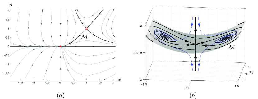
Figure 1: Simple examples illustrating the need to extend the primary SSMs used in nonlinear model reduction to a more general family of invariant manifolds (a) The phase portrait of system (1) for $a=b=1$ and $c=2.5$. (b) The phase space geometry of system (2) for $k=\sqrt{2}/2$, $a=0.5$ and $c=0.2$.

A Galerkin projection onto POD modes does not produce a feasible reduced-order model for this simple problem, as we show in Appendix A of the Supplementary Material. Linear data-driven techniques, such as DMD and its variants (Schmid [57]), are clearly unable to capture simultaneously the two fixed points and the orbit connecting them, as was explicitly illustrated in the context of Couette flows by Page and Kerswell [50].

The slow SSM of the origin, i.e., the unique smoothest nonlinear continuation of the slower eigenspace, is the $x$ axis, on which the reduced dynamics is $\dot{x}=-bx$. This gives a correct reduced-order model for the asymptotic behavior of all trajectories in the domain of attraction of the origin, yet fails to provide any information about the truly nonlinear dynamics. This is undesirable as both the coexisting saddle point and the separatrix $\mathcal{M}$ connecting it to the origin can be brought arbitrarily close to the origin by selecting small enough values for the parameters $a$ and $b$.

A simple calculation reveals that any trajectory of the linear part of (1) can be written as a graph $y=K\left|x\right|^{\frac{ac}{b}}$ for some choice of the parameter $K\in\mathbb{R}$. This suggest that the manifold $\mathcal{M}$ containing the two fixed points may also just be $\left[\frac{ac}{b}\right]$ times differentiable at the origin, with the brackets referring to the integer part of a real number. Our first main objective in this paper is to establish the general existence and smoothness of secondary SSMs like $\mathcal{M}$ in nonlinear dynamical systems and obtain data-driven reduced models on such manifolds. These SSMs, however, turn out to lie outside the scope of usual equation- and data-driven approximation methods that use polynomials with integer powers. As we will see for this example in Appendix A of the Supplementary material, use of fractional SSMs enables the data-driven construction for an accurate 1D reduced-order model for trajectories near the transition orbit. Additionally, we will show for the planar Couette flow in Section 6 that use of fractional SSMs increases the accuracy of the SSM-reduced model without the inclusion of higher-order terms in that model.

As a second example, consider the system

$$\dot{x}_{1} =x_{2},$$

$$\dot{x}_{2} =x_{1}-cx_{2}-x_{1}^{3},$$

$$\dot{x}_{3} =-kx_{3}+kax_{1}^{2}+2ax_{1}x_{2}.$$ (2)

for which $\mathcal{M}=\left\{x\in\mathbb{R}^{3}\colon x_{3}=ax_{1}^{2}\right\}$ is a unique, two-dimensional (2D), attracting $C^{\infty}$ invariant manifold that is tangent to the $x_{3}=0$ spectral subspace. Within this manifold, the restricted dynamics is just that of a damped Duffing oscillator with two stable spirals and one saddle point at the origin, as shown in Fig. 1b.

The $x_{3}=0$ spectral subspace contains both a stable and an unstable eigenvector of the origin, and hence the results of Cabré et al. [13] are not applicable to conclude the existence of $\mathcal{M}$ purely based on the spectrum of the linearized ODE at the origin. The more classic result of Irwin on pseudo-unstable manifolds (de la Llave and Wayne [23]) do not apply for the parameter values used in Fig. 1 (see Appendix B of the Supplementary Material). Our second main objective in this paper is to derive reduced-order models on secondary SSMs such as $\mathcal{M}$ in Fig. 1b. As we will see in Section 7, an important physical application of such mixed-mode SSMs is the reduced-order modeling of dynamic buckling of beams.

3 Generalized SSMs near fixed points of autonomous dynamical systems

We consider a smooth system of $n$-dimensional ODEs of the form

$$\dot{x}=\mathcal{A}x+f(x),\qquad x\in\mathbb{R}^{n},\quad\mathcal{A}\in\mathbb{R}^{n\times n},\quad f=\mathcal{O}\left(\left|x\right|^{2}\right)\in C^{\infty},\qquad 1\leq n<\infty,$$ (3)

and assume that its fixed point at $x=0$ is hyperbolic, i.e., the spectrum $\mathrm{spect}\left(\mathcal{A}\right)=\left\{\lambda_{1},\ldots,\lambda_{n}\right\}$ of $\mathcal{A}$ satisfies

$$0\notin\mathrm{Re}\left[\mathrm{spect}\left(\mathcal{A}\right)\right],$$ (4)

with $\mathrm{Re}\left[\mathrm{spect}\left(\mathcal{A}\right)\right]$ denoting the real part of the spectrum of the linear operator $\mathcal{A}$. We note that the $C^{\infty}$ assumption on $f$ can be relaxed to finite smoothness if $\mathrm{Re}\left[\mathrm{spect}\left(\mathcal{A}\right)\right]\subset(-\infty,0)$ or $\mathrm{Re}\left[\mathrm{spect}\left(\mathcal{A}\right)\right]\subset(0,\infty)$ holds (see statement (v) of Theorem 1). We also note that our results in Section 4 will also allow for the addition of small time-periodic forcing term to (3) (see Remark 10).

We further assume that $\mathcal{A}$ is semisimple, i.e., the geometric and algebraic multiplicities of any potential repeated eigenvalue of $\mathcal{A}$ are equal. This is generally true for physical oscillatory systems in which possible repeated eigenvalues arise from symmetry and hence each eigenvalue has its own associated oscillatory mode generated by an independent eigenvector. We finally assume that with the exception of possible $1\colon 1$ resonances created by repeated eigenvalues of $\mathcal{A}$, there are no further resonances within $\mathrm{spect}\left(\mathcal{A}\right)$, i.e., we have

$$\lambda_{j}\neq\sum_{k=1}^{n}m_{k}\lambda_{k},\quad m_{k}\in\mathbb{N},\quad\sum_{k=1}^{n}m_{k}\geq 2,\quad j=1,\ldots,n.$$ (5)

While these nonresonance conditions will typically hold for generic parameter configurations of typical dissipative systems, they can easily fail on simple toy examples with non-generic parameter choices. For instance, a simple 2D saddle-type fixed point with eigenvalues $\lambda_{1}=-1$ and $\lambda_{2}=1$ will violate infinitely many of the conditions (5) for $j=1$, $m_{1}=m_{2}+1$ and $j=2$, $m_{2}=m_{1}+1$. The main motivation for the present paper is the data-driven modeling of dissipative physical systems in which such exceptional parameter configurations are unlikely. We stress, however, that repeated eigenvalues arising from a physical symmetry are not excluded by conditions (5).

We now select and fix an arbitrary spectral subspace $E\subset\mathbb{R}^{n}$ of $\mathcal{A}$ and seek to find its nonlinear continuation in the full system (3). In practical terms, we are interested in nonlinear interactions along which all modes can be enslaved to a set of linear master modes spanning $E$. We assume that $\mathrm{spect}\left(\mathcal{A}|_{E}\right)$ contains $p$ purely real eigenvalues and $q$ pairs of complex conjugate eigenvalues. Similarly, we assume that $\mathrm{spect}\left(\mathcal{A}\right)-\mathrm{spect}\left(\mathcal{A}|_{E}\right)$ contains $r$ purely real eigenvalues and $s$ pairs of complex conjugate eigenvalues. In that case, after a linear change of coordinates, we can assume a partition of the $x$ coordinate in the form

$$x=\left(u,\left(a_{1},b_{1}\right),\ldots,\left(a_{q},b_{q}\right),v,\left(c_{1},d_{1}\right),\ldots,\left(c_{s},d_{s}\right)\right)\in\mathbb{R}^{p}\times\underbrace{\mathbb{R}^{2}\times\ldots\times\mathbb{R}^{2}}_{q}\times\mathbb{R}^{r}\times\underbrace{\mathbb{R}^{2}\times\ldots\times\mathbb{R}^{2}}_{s},$$ (6)

with $\quad p+2q+r+2s=n,$ in which the coefficient matrix $\mathcal{A}$ of the linear part of system (3) takes its real Jordan canonical form

$$\mathcal{A}=\mathrm{diag}\left[A,B_{1},\ldots,B_{q},C,D_{1},\ldots,D_{s}\right],$$ (7)

with

$$A =\mathrm{diag}\left[\lambda_{1},\ldots,\lambda_{p}\right]\in\mathbb{R}^{p\times p},\quad B_{k}=\left(\begin{array}[]{cc}\alpha_{k}&-\omega_{k}\\ \omega_{k}&\alpha_{k}\end{array}\right)\in\mathbb{R}^{2\times 2},\quad k=1,\ldots,q,$$ (10)

$$C =\mathrm{diag}\left[\kappa_{1},\ldots,\kappa_{r}\right]\in\mathbb{R}^{r\times r},\quad D_{m}=\left(\begin{array}[]{cc}\beta_{m}&-\nu_{m}\\ \nu_{m}&\beta_{m}\end{array}\right)\in\mathbb{R}^{2\times 2},\quad m=1,\ldots,s.$$ (13)

Some of the eigenvalues $\lambda_{j},$ $\alpha_{k}+i\omega_{k}$, $\kappa_{\ell}$ and $\beta_{m}+i\nu_{m}$ in the spectrum of $\mathcal{A}$ may be repeated, as $1:1$ resonances are allowed by the nonresonance conditions (5).

Our main result is the simplest to state in complexified coordinates. To this end, we introduce the variables

$$z=a+ib\in\mathbb{C}^{q},\quad w=c+id\in\mathbb{C}^{s},$$ (14)

and the piecewise constant functions

$$K_{\ell j}(\zeta)=\left\{\begin{array}[]{c}K_{\ell j}^{+}\qquad\zeta>0,\\ \\ K_{\ell j}^{-}\qquad\zeta\leq 0,\end{array}\right.\qquad O_{mj}(\zeta)=\left\{\begin{array}[]{c}O_{mj}^{+}\qquad\zeta>0,\\ \\ O_{mj}^{-}\qquad\zeta\leq 0,\end{array}\right.$$ (15)

with constant families $K_{\ell j}^{\pm}\in\mathbb{R}$ and $O_{mj}^{\pm}\in\mathbb{C}$. We also define the continuous function families

$$\mathcal{V}_{\ell}(u,z) =\sum_{j=1}^{p}K_{\ell j}(u_{j})\left|u_{j}\right|^{\frac{\kappa_{\ell}}{\lambda_{j}}}+\sum_{k=1}^{q}L_{\ell k}\left|z_{k}\right|^{\frac{\kappa_{\ell}}{\alpha_{k}}},\quad\ell=1,\ldots,r,$$

$$\mathcal{\mathcal{E}}_{m}(u,z) =\left[\sum_{j=1}^{p}O_{mj}(u_{j})\left|u_{j}\right|^{\frac{\beta_{m}}{\lambda_{j}}}+\sum_{k=1}^{q}Q_{mk}\left|z_{k}\right|^{\frac{\beta_{m}}{\alpha_{k}}}\right]e^{i\left(\sum_{j=1}^{p}\frac{\nu_{m}}{\lambda_{j}}\log\left|u_{j}\right|+\sum_{k=1}^{q}\frac{\nu_{m}}{\alpha_{k}}\log\left|z_{k}\right|\right)},\quad m=1,\ldots,s,$$

where $Q_{mk}\in\mathbb{C}$ and

$$K_{\ell j} (u_{j})\equiv 0,\quad\mathrm{if}\quad\frac{\kappa_{\ell}}{\lambda_{j}}<0,\qquad O_{mj}(u_{j})\equiv 0,\quad\mathrm{if}\quad\frac{\beta_{m}}{\lambda_{j}}<0,$$

$$L_{\ell k} =0,\quad\mathrm{if}\quad\frac{\kappa_{\ell}}{\alpha_{k}}<0,\qquad Q_{mk}=0,\quad\mathrm{if}\quad\frac{\beta_{m}}{\alpha_{k}}<0.$$ (17)

As seen in the proof of our upcoming main theorem, the function families (LABEL:eq:complex_SSM_1) describe all continuous invariant graphs over $E$ in the linear part of system (3).

For any positive integer $N$, any vector $e\in\mathbb{C}^{N}$ and nonnegative integer vector $\mathbf{k}\in\mathbb{N}^{N}$, we will use the notation

$$e^{\mathbf{k}}:=e_{1}^{k_{1}}e_{2}^{k_{2}}\cdot\ldots\cdot e_{N}^{k_{N}}\in\mathbb{C}.$$

Finally, we will use the notation

$$\sum_{2\leq\mathrm{monomial}\mathrm{\,order}\leq\mathcal{K}}M_{\mathbf{k}}\left(u,z\right)$$ (18)

for expansions involving monomials $M_{\mathbf{k}}\left(u,z\right)$ of general positive (but potentially fractional) powers of $u$ and $z$. These monomials will be indexed by a multi-index $\mathbf{k}\in\mathbb{N}^{p+2q+r+2s}$ but their order (referred to as monomial order) will be a homogeneous linear function of $\mathbf{k}$, rather than $\mathbf{k}$ itself. We will explicitly write out the monomial order as functions in simpler settings (see, e.g., Propositions 1 and 2) in which the notation does not become too involved.

With these definitions, our main result can be stated as follows.

Theorem 1.

(i)

For any integer order $\mathcal{K}\geq 2$ of approximation, there exists a unique set of coefficients $h_{\mathbf{k}}\in\mathbb{C}^{r+s}$ such that the full family $\mathcal{W}\left(E\right)$ of SSMs tangent to the spectral subspace $E$ of the nonlinear system (3) can locally be written near the origin as

$$\left(\begin{array}[]{c}v\\ w\end{array}\right) =\mathcal{G}(u,z)=\left(\begin{array}[]{c}\mathcal{V}(u,z)\\ \mathcal{\mathcal{E}}(u,z)\end{array}\right)+\sum_{2\leq\mathrm{monomial}\mathrm{\,order}\leq\mathcal{K}}h_{\mathbf{k}}u^{\mathbf{k}_{1}}z^{\mathbf{k}_{2}}\bar{z}^{\mathbf{k}_{3}}\mathcal{V}^{\mathbf{k}_{4}}\mathcal{\mathcal{E}}^{\mathbf{k}_{5}}\bar{\mathcal{\mathcal{E}}}^{\mathbf{k}_{6}}+o\left(\left|\left(u,z\right)\right|^{\mathcal{K}}\right),$$ (23)

$$\,\,\,\,\,\,\mathbf{k}_{1}\in\mathbb{N}^{p},\quad\mathbf{k}_{2},\mathbf{k}_{3}\in\mathbb{N}^{q},\quad\mathbf{k}_{4}\in\mathbb{N}^{r},\quad\mathbf{k}_{5},\mathbf{k}_{6}\in\mathbb{N}^{s},\quad\mathbf{k}=\left(\mathbf{k}_{1},\mathbf{k}_{2},\mathbf{k}_{3},\mathbf{k}_{4},\mathbf{k}_{5},\mathbf{k}_{6}\right),$$

where $\mathcal{V}(u,z)\in\mathbb{R}^{r}$ and $\mathcal{\mathcal{E}}(u,z)\in\mathbb{C}^{s}$ are defined via formulas (LABEL:eq:complex_SSM_1), with $K_{\ell j}$, $O_{mj}$, $L_{\ell k}$ and $Q_{mk}$ satisfying the constraints (17) but otherwise chosen arbitrarily.

(ii)

The reduced dynamics on the individual members of the family $\mathcal{W}\left(E\right)$ are given by

$$\left(\begin{array}[]{c}\dot{u}\\ \dot{z}\end{array}\right)=\left(\begin{array}[]{cccc}A&0&0&0\\ 0&B_{1}&0&0\\ 0&0&\ddots&0\\ 0&0&0&B_{q}\end{array}\right)\left(\begin{array}[]{c}u\\ z\end{array}\right)+f^{\left(u,z\right)}\left(u,z,\mathcal{G}(u,z)\right),$$ (24)

where $f^{\left(u,z\right)}$ denotes the $(u,z)$ coordinate component of $f=\left(f^{\left(u,z\right)},f^{v},f^{w}\right)$.

(iii)

If and

$$\frac{\kappa_{\ell}}{\lambda_{j}}<0,\qquad\frac{\beta_{m}}{\lambda_{j}}<0,\qquad\frac{\kappa_{\ell}}{\alpha_{k}}<0,\qquad\frac{\beta_{m}}{\alpha_{k}}<0$$ (25)

hold for all values of the indices $j,k,\ell$ and $m$, then $\mathcal{W}\left(E\right)$ is unique and of class $C^{\infty}$. Otherwise, $\mathcal{W}\left(E\right)$ is a family of non-unique SSMs whose typical member is of smoothness class $C^{\eta}$ with

$$\eta=\mathrm{Int}\left[\min_{j,k,\ell,m}^{+}\left\{\frac{\kappa_{\ell}}{\lambda_{j}},\quad\frac{\beta_{m}}{\lambda_{j}},\quad\frac{\kappa_{\ell}}{\alpha_{k}},\quad\frac{\beta_{m}}{\alpha_{k}}\right\}\right],$$ (26)

where the $\mathrm{Int}$ refers to the integer part of a positive number and $\min^{+}$ refers to a minimum of the positive elements of a list of numbers that follow. Even in that case, however, there exists a unique member $\mathcal{W}^{\infty}(E)$ of the SSM family that is of class $C^{\infty}$ and satisfies $K_{\ell j}^{\pm}\equiv O_{mj}^{\pm}=L_{\ell k}=Q_{mk}=0$ for all $j,k,\ell$ and $m$ in eq. (LABEL:eq:complex_SSM_1).

(iv)

If system (23) is $C^{R}$ in a parameter vector $\mu\in\mathbb{R}^{P}$, then $\mathcal{W}\left(E\right)$ is also $C^{R}$ in $\mu$.

(v)

If the function $f$ only has finite smoothness, i.e., $f=\mathcal{O}\left(\left|x\right|^{2}\right)\in C^{\rho}$ and $\mathrm{Re\,\lambda_{j}}$ has the same nonzero sign for all $j=1,\ldots,N$, then statements (i)-(iv) still hold for all $\mathcal{K}\leq\rho$.

(vi)

If the function $f$ is analytic in a neighborhood of the origin and $\mathrm{Re\,\lambda_{j}}$ has the same nonzero sign for all $j=1,\ldots,N$, then the series expansion (23) converges near the origin as $\mathcal{K}\to\infty$.

Proof.

See Appendix C of the Supplementary Material. ∎

Remark 1.

[Relation to primary SSMs] We note that to obtain classical stable and unstable manifolds as well as the primary (smoothest) SSMs defined by Haller and Ponsioen [33], all constants $K_{\ell j}$, $O_{mj}$, $L_{\ell k}$ and $Q_{mk}$ in the definitions (LABEL:eq:complex_SSM_1) have to be set to zero and the signs of all $\lambda_{j}$ and $\alpha_{k}$ involved must be the same. In contrast, the full family of invariant manifolds covered by Theorem 1 is significantly larger and includes secondary (fractional and mixed-mode) SSMs. The existing open-source SSMLearn package of Cenedese et al. [18] can be used to compute primary mixed-mode SSMs as well, even though the SSM theory originally supporting that package was only available for fixed points that are asymptotically stable in forward or backward time. This is because the integer-powered polynomial expansions for mixed-mode SSMs satisfy the same type of invariance equations as their like-mode counterparts and hence can be approximated from data in the same fashion.

Remark 2.

[Relation to non-linearizable dynamics] Increasing $\mathcal{K}$ in the general formula (23) generally decreases the size of the open neighborhood of the origin in which this representation of the SSM family is valid. Specifically, in the limit of $\mathcal{K}\to\infty$, only the part of the SSM family $\mathcal{W}\left(E\right)$ is captured by formula (23) that carries linearizable dynamics, given that the main tool used in obtaining this asymptotic limit of this formula is the $C^{\infty}$ linearization result of Sternberg [63]. In contrast, using a finite $\mathcal{K}$ in a data-driven identification of $\mathcal{W}\left(E\right)$ enables the accurate approximation of SSMs on larger domains containing non-linearizable dynamics, such as coexisting isolated compact invariant sets and transitions among them. We will illustrate this on specific examples in Sections 6-8.

Remark 3.

[Resonances] As noted after formula (5), $1\colon 1$ resonances are allowed among the eigenvalues of $\mathcal{A}$ by the assumptions of Theorem 1. For other resonances, the nonresonance condition (5) is substantially less restrictive than what one might be used to in the classical vibrations literature. For instance, $2\lambda_{1}=3\lambda_{2}$ satisfies condition (5) and hence is not a resonance in our discussion unless further matches arise with the remaining eigenvalues, which has low probability in a physical system. Similarly, the case $\mathrm{Im}\lambda_{1}=3$$\mathrm{Im}\lambda_{2}$ is considered a $1:3$ frequency-resonance in the nonlinear vibrations literature, but it is only a resonance in the sense of formula (5) if we also have the same resonance between the decay rates of the two corresponding modes, i.e., $\mathrm{Re}\lambda_{1}=3\mathrm{Re}\lambda_{2}$ holds simultaneously. This is again highly unlikely for physical system, especially in the data driven setting. If eigenvalue relations violating (5) do need to be considered for some reason, then primary, like-mode SSMs defined over spectral subspaces incorporating the resonant eigenvectors still exist by the theory of Cabré et al. [13] (see Li et al. [45, 46] for specific examples). Finally, under resonances of order $\sum_{k=1}^{n}m_{k}>\mathcal{K}$, formula (23) still provides an an expression for an approximately invariant manifold with invariance error of $o\left(\left|\left(u,z\right)\right|^{\mathcal{K}}\right)$. This follows from the fact that a finite polynomial (and hence analytic) transformation linearizing the system up to order $\mathcal{K}$ still exists. In a data-driven setting, such a small error in locating invariant manifolds is generally unavoidable for higher values of $\mathcal{K}$ even in the absence of resonances.

Remark 4.

[Constraints on parameters] The constraints on the parameters in (17) are relevant when the stability types of the eigenvectors aligned with $v_{\ell}$ is the opposite of those aligned with $u_{j}$ or $z_{k}$, in which case any non-flat invariant graph over $E$ blows up at the origin. If contrast, if $\frac{\kappa_{\ell}}{\lambda_{j}}>0$ and $\frac{\kappa_{\ell}}{\alpha_{k}}>0$ hold, then any nonzero $K_{\ell j}^{\pm}$ and $L_{\ell k}$ are allowed in the expression (LABEL:eq:complex_SSM_1).

Remark 5.

[Generic smoothness in the $\mathcal{W}\left(E\right)$ family] Statement of (iii) of Theorem 1 specifies the order $\eta$ of differentiability of a generic fractional SSM in the family of $\mathcal{W}\left(E\right)$. For such generic members of the family, all coefficients appearing in the definition (LABEL:eq:complex_SSM_1) of the functions $\mathcal{V}$ and $\mathcal{E}$ are nonzero. Nongeneric subfamilies of the $\mathcal{W}\left(E\right)$ family will have higher smoothness classes equal to the integer part of one of the positive members in the list of quotients in formula (26). However, as we illustrate in Fig. 2 on a specific case, these nongeneric subfamilies form measure zero, nowhere dense subsets of the full $\mathcal{W}\left(E\right)$ family.

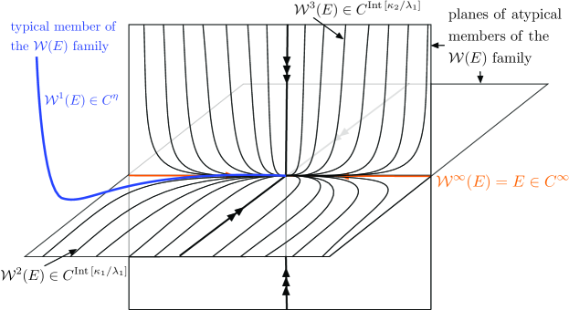
Figure 2: Various members of the SSM family $\mathcal{W}(E)$ in the case of $j=1$ , $k=0$, $\ell=1$ and $m=0$, shown after a $C^{\infty}$ linearizing transformation near the origin has been performed (see the proof of Theorem 1). $\mathcal{W}^{\infty}(E)=E$: unique member of smoothness class $C^{\infty}$ ; $\mathcal{W}^{1}(E)$: generic member of smoothness class $C^{\eta}$; $\mathcal{W}^{2}(E)$: nongeneric member of smoothness class $C^{\mathrm{Int}\,\left[\kappa_{1}/\lambda_{1}\right]}$ ; $\mathcal{W}^{3}(E)$: nongeneric member of class $C^{\mathrm{Int}\,\left[\kappa_{2}/\lambda_{1}\right]}$ .

Finally, by their construction in the proof of Theorem 1, generic members of the fractional SSM family $\mathcal{W}\left(E\right)$ guaranteed by statement (i) of the theorem are actually always of class $C^{\infty}$ away from the origin. At the origin, their Hölder smoothness class is $C^{\eta,\alpha}$ for some $0\leq\alpha<1$.

Remark 6.

[Use of piecewise constant coefficients] The use of the piecewise constant functions (15) enables us to pair up arbitrary positive and negative branches of fractional SSMs to obtain a single, continuous invariant manifold. This is illustrated in Fig. 3 for the linear part of system (3) which already exhibits the same geometry. Replacing the function $K_{\ell j}(u_{j})$ simply with a single constant $K_{\ell j}$ is possible but limits the general family of graphs to symmetric ones, as seen in Fig. 3. The same observation is valid for $O_{mj}(u_{j})$.

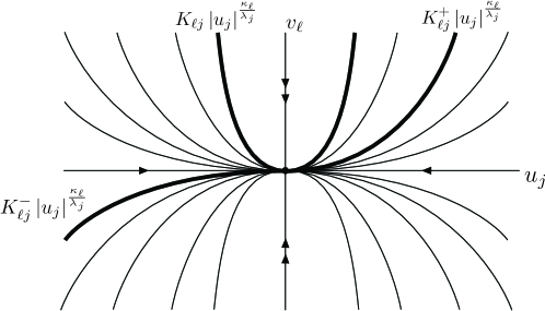
Figure 3: Infinitely many invariant graphs (fractional SSMs) of smoothness class $C^{\mathrm{int}\left[\frac{\kappa_{\ell}}{\lambda_{j}}\right]}$ pass through any point of the $(u_{j},v_{\ell})$ plane in the linear part of system (3). The symmetric members of this family are of the form $v_{\ell}=K_{\ell j}\left|u_{j}\right|^{\frac{\kappa_{\ell}}{\lambda_{j}}}$ while the asymmetric members are of the general form $v_{\ell}=K_{\ell j}(u_{j})\left|u_{j}\right|^{\frac{\kappa_{\ell}}{\lambda_{j}}}$. The single $C^{\infty}$ invariant graph (primary SSM) over the $u_{j}$ axis is the $u_{j}$ axis itself.

Remark 7.

[Data-driven construction of fractional and mixed-mode SSMs] Primary mixed-mode SSMs require no detailed information on the spectrum of $\mathcal{A}$ outside their underlying spectral eigenspaces. For this reason, mixed-mode SSMs can be directly constructed from data featuring decaying nonlinear oscillations near $E$ via the open source Matlab codes SSMLearn and fastSSM developed by Cenedese et al. [19] and Axås et al. [6] (see https://github.com/haller-group). In contrast, the construction of fractional SSMs requires decay-rate information both inside and outside $E$, the latter of which is not immediately recognizable from decaying oscillation data near $E$. In the Conclusions section, we mention a few data-driven strategies to obtain this spectral information external to $E$. Once this information is available, the construction of mixed-mode SSMs follows the same algorithm used in SSMLearn and fastSSM but with the fractional-powered terms added to the integer-powered representation of the invariant manifolds. If, however, some of the fractional powers appearing in the formulas (LABEL:eq:complex_SSM_1) are close to integers, then those fractional terms are advisable to omit in a data-driven construction of the SSM to avoid an overfit. All these steps in a data-driven implementation of Theorem 1 are currently under development and will appear elsewhere. In all our upcoming examples in Sections 6-8, we obtain linear spectral information outside $E$ from the governing equations but construct the fractional and mixed-mode manifolds in a data-driven fashion, using only numerically generated solutions of those governing equations.

Remark 8.

[Uniqueness of invariant manifolds] The $C^{\infty}$ linearizing conjugacies of Sternberg [63] used in proving Theorem 1 have only been known to be unique under the assumptions of statement (v) of the theorem (Kvalheim and Revzen [41]). This, however, does not affect the uniqueness of $\mathcal{W}^{\infty}(E)$ or the uniqueness of the members of the full SSM family $\mathcal{W}(E)$. Indeed, as members of $\mathcal{W}(E)$ provide a well-defined foliation by invariant surfaces of a full neighborhood of the origin under a given $C^{\infty}$ linearizing conjugacy, another $C^{\infty}$ linearization conjugacy cannot change the elements and their smoothness in this foliation without violating their invariance. Only the specific parametrization of the fractional and primary SSMs in $\mathcal{W}(E)$ can change when one picks another linearizing conjugacy. This is also the reason behind the uniqueness of $\mathcal{W}\left(E\right)$ in statement (iii), given that conditions (25) cause the linearized system to have a unique continuous invariant manifold ($E$ itself) that is tangent to $E$ at the origin and has the same dimension as $E$. This manifold then has the same unique $C^{\infty}$ preimage under any $C^{\infty}$ linearizing transformation, and hence the corresponding $\mathcal{W}\left(E\right)$ is a unique manifold in the nonlinear system (2).

Remark 9.

[Choice of the dimension of the SSM] Theorem 1 provides a hierarchical chain of SSM families, $W\left(E_{1}\right)\subset W\left(E_{2}\right)\subset\ldots\subset W\left(E_{n-1}\right)$, with each family acting as a nonlinear, invariant continuation of a corresponding spectral subspace in the hierarchical chain $E_{1}\subset E_{2}\subset\ldots\subset E_{n-1}$ of spectral subspaces. In applications, the asymptotic dynamics are generally captured by the slowest family $W\left(E_{1}\right)$ of these SSM families. If predictions are required for shorter time scales as well, one can gradually increase the size of the family by considering $W\left(E_{k}\right)$ under increasing $k.$ This procedure includes more and more of the transient dynamics while keeping the core asymptotic dynamics unchanged. One reason for considering $W\left(E_{k}\right)$ with $k>1$ in a data-driven setting is if the data shows significant interaction of the first mode with higher modes up to order $k$. In most practical applications of SSMs with larger spectral gaps, however, including the lowest-order primary SSM suffices (see Cenedese et al. [19] and Cenedese et al. [20]). A similar experience is emerging from applications of SSMs in model-predictive control of soft robots, where a two-dimensional SSM constructed along each spatial degree of freedom already provides a highly accurate reduced-order model (see Alora et al. [2]).

The simplest case in applications is wherein $E$ is 1D ($p=1$, $q=0$), and there are also $r$ further non-oscillatory modes of the same stability type ($s=0$). For that case, Theorem 1 takes the following more specific form.

Proposition 1.

Assume that $p=1$, $q=0$ and $s=0$ hold. Then, for any integer order $\mathcal{K}\geq 2$ of approximation, the full family $\mathcal{W}\left(E\right)$ of SSMs tangent to the spectral subspace $E$ of the nonlinear system (3) can locally be written as

$$v =\sum_{1\leq k_{1}+\sum_{\ell=1}^{r}k_{4\ell}\frac{\kappa_{\ell}}{\lambda_{1}}\leq\mathcal{K}}C_{\mathbf{k}}(u_{1})u_{1}^{k_{1}}\left|u_{1}\right|^{\sum_{\ell=1}^{r}k_{4\ell}\frac{\kappa_{\ell}}{\lambda_{1}}}+o\left(\left|u_{1}\right|^{\mathcal{K}}\right),$$ (27)

with the arbitrary, piecewise constant functions $C_{\mathbf{k}}(u_{1})\in\mathbb{R}^{r}$ satisfying

$$C_{\mathbf{k}\ell}(u_{1})=\left\{\begin{array}[]{c}C_{\mathbf{k}\ell}^{+}\qquad u_{1}>0,\\ \\ C_{\mathbf{k}\ell}^{-}\qquad u_{1}\leq 0,\end{array}\right.\qquad C_{\mathbf{k}\ell}^{\pm}=0:\quad\frac{\kappa_{\ell}}{\lambda_{1}}<0\,\,\,\,\,\,\,\mathrm{or}\,\,\,\,\,\left|\mathbf{k}\right|=1,\,\,k_{4\ell}\neq 1,\,\qquad\ell=1,\ldots,r.$$

Proof.

See Appendix D of the Supplementary Material. ∎

Note that for the primary (smoothest) SSM in the $\mathcal{W}\left(E\right)$ family covered by Proposition 1, there exists a unique parameter vector sequence $C_{\mathbf{k}}$ with $k_{1}\geq 2$ and $\mathbf{k}_{4}=\mathbf{0}$.

Another frequent case in practice is wherein $E$ is 2D, carries oscillations ($p=0$, $q=1$), and there are also $s$ further oscillatory modes ($r=0$). For that case, Theorem 1 takes the following more specific form.

Proposition 2.

Assume that $p=0$, $q=1$ and $r=0$ hold. Then, for any integer order $\mathcal{K}\geq 2$ of approximation, the full family $\mathcal{W}\left(E\right)$ of SSMs tangent to the spectral subspace $E$ of the nonlinear system (3) can locally be written as

$$w =\sum_{1\leq k_{2}+k_{3}+\sum_{m=1}^{s}\left(k_{5m}+k_{6m}\right)\frac{\beta_{m}}{\alpha_{1}}\leq\mathcal{K}}D_{\mathbf{k}}z_{1}^{k_{2}}\bar{z}_{1}^{k_{3}}\left|z_{1}\right|^{\sum_{m=1}^{s}\left(k_{5m}+k_{6m}\right)\frac{\beta_{m}}{\alpha_{1}}}e^{i\sum_{m=1}^{s}\left(k_{5m}-k_{6m}\right)\frac{\nu_{m}}{\alpha_{1}}\log\left|z_{1}\right|}$$ (28)

$$+o\left(\left|z_{1}\right|^{\mathcal{K}}\right),$$ (29)

$$\,\,\,\,\,\,k_{2},k_{3}\in\mathbb{N},\quad\mathbf{k}_{5},\mathbf{k}_{6}\in\mathbb{N}^{s},\quad\mathbf{k}=\left(k_{2},k_{3},\mathbf{k}_{5},\mathbf{k}_{6}\right),$$

with the arbitrary constants $D_{\mathbf{k}}\in\mathbb{C}^{s}$ satisfying

$$D_{\mathbf{k}m}=0:\quad\frac{\beta_{m}}{\alpha_{1}}<0\,\,\,\,\,\,\mathrm{or}\,\,\,\,\,\,\,\left|\mathbf{k}\right|=1,k_{5m}\neq 1,\qquad m=1,\ldots,s.$$

Proof.

See Appendix D of the Supplementary Material. ∎

Note that for the primary SSM $\mathcal{W}^{\infty}(E)$ in the $\mathcal{W}\left(E\right)$ family covered by Proposition 2, there exists a unique parameter vector sequence $D_{\mathbf{k}}$ with $\left|\mathbf{k}\right|\geq 2$, $\mathbf{k}_{5}=\mathbf{k}_{6}=\mathbf{0}$.

4 Generalized SSMs near fixed points of discrete dynamical systems

The techniques and prior results used in the proof of Theorem 1 are also applicable with appropriate modifications to discrete dynamical systems defined by iterated mappings. This enables us to derive generalized SSM results for sampled data sets of autonomous dynamical systems and for the Poincaré maps of time-periodically forced dynamical systems. The latter extension, in turn, implies the existence of time-periodic generalized SSMs along periodic orbits of such systems. We only list the related results for maps in this section with their proofs relegated to appendices in the Supplementary Material.

We consider an iterated nonlinear mapping of the form

$$x(\imath+1)=\mathcal{A}x(\imath)+f\left(x(\imath)\right),\qquad x\in\mathbb{R}^{n},\quad\mathcal{A}\in\mathbb{R}^{n\times n},\quad f=\mathcal{O}\left(\left|x\right|^{2}\right)\in C^{\infty},\qquad 1\leq n<\infty,$$ (30)

and assume that its fixed point at $x=0$ is hyperbolic, i.e., the spectrum $\mathrm{spect}\left(\mathcal{A}\right)=\left\{\lambda_{1},\ldots,\lambda_{n}\right\}$ of $\mathcal{A}$ satisfies

$$\mathrm{spect}\left(\mathcal{A}\right)\cap\left\{\lambda\in\mathbb{C}:\,\,\left|\lambda\right|=1\right\}=\emptyset.$$ (31)

As in the case of continuous dynamical systems, we can also allow $f$ to be of finite smoothness if $\mathrm{spect}\left(\mathcal{A}\right)$ is fully inside or fully outside the complex unit circle (see Theorem 2).

We again assume that $\mathcal{A}$ is semisimple and the following nonresonance conditions hold among its eigenvalues:

$$\lambda_{j}\neq\prod_{k=1}^{n}\lambda_{k}^{m_{k}},\quad m_{k}\in\mathbb{N},\quad\sum_{k=1}^{n}m_{k}\geq 2,\quad j=1,\ldots,n.$$ (32)

As in the case of continuous dynamical systems that we have already treated, repeated eigenvalues arising from a physical symmetry are not excluded by conditions (32).

We select and fix an arbitrary spectral subspace $E\subset\mathbb{R}^{n}$ and assume that the spectrum of $\mathcal{A}|_{E}$ contains $p$ purely real eigenvalues and $q$ pairs of complex conjugate eigenvalues. Similarly, we assume that the remainder of the spectrum of $\mathcal{A}$ contains $r$ purely real eigenvalues and $s$ pairs of complex conjugate eigenvalues. In that case, possibly after a linear change of coordinates, we can assume a partition of the $x$ coordinate in the form

$$x=\left(u,\left(a_{1},b_{1}\right),\ldots,\left(a_{q},b_{q}\right),v,\left(c_{1},d_{1}\right),\ldots,\left(c_{s},d_{s}\right)\right)\in\mathbb{R}^{p}\times\underbrace{\mathbb{R}^{2}\times\ldots\times\mathbb{R}^{2}}_{q}\times\mathbb{R}^{r}\times\underbrace{\mathbb{R}^{2}\times\ldots\times\mathbb{R}^{2}}_{s},$$ (33)

with $\quad p+2q+r+2s=n,$ in which the coefficient matrix $\mathcal{A}$ of the linear part of system (30) takes its real Jordan canonical form

$$\mathcal{A}=\mathrm{diag}\left[A,B_{1},\ldots,B_{q},C,D_{1},\ldots,D_{s}\right],$$ (34)

where

$$A =\mathrm{diag}\left[\lambda_{1},\ldots,\lambda_{p}\right]\in\mathbb{R}^{p\times p},\quad B_{k}=\left(\begin{array}[]{cc}\alpha_{k}&-\omega_{k}\\ \omega_{k}&\alpha_{k}\end{array}\right)\in\mathbb{R}^{2\times 2},\quad k=1,\ldots,q,$$ (37)

$$C =\mathrm{diag}\left[\kappa_{1},\ldots,\kappa_{r}\right]\in\mathbb{R}^{r\times r},\quad D_{m}=\left(\begin{array}[]{cc}\beta_{m}&-\nu_{m}\\ \nu_{m}&\beta_{m}\end{array}\right)\in\mathbb{R}^{2\times 2},\quad m=1,\ldots,s.$$ (40)

To simplify our final formulas, we also assume that

$$\kappa_{\ell}>0,\quad\ell=1,\ldots,r,$$ (41)

which means that the linearized mapping is orientation preserving along all of the $v_{\ell}$ directions.

Using again the complexified variables $z=a+ib\in\mathbb{C}^{q}$ and $w=c+id\in\mathbb{C}^{s}$, as well as the piecewise constant functions (15), we define the discrete analogues of formulas (LABEL:eq:complex_SSM_1) as

$$\mathcal{V}_{\ell}(u,z) =\sum_{j=1}^{p}K_{\ell j}\left(u_{j}\right)\left|u_{j}\right|^{\frac{\log\kappa_{\ell}}{\log\left|\lambda_{j}\right|}}+\sum_{k=1}^{q}L_{\ell k}\left|z_{k}\right|^{\frac{\log\kappa_{\ell}}{\log\sqrt{\alpha_{k}^{2}+\omega_{k}^{2}}}},\quad\ell=1,\ldots,r,$$

$$\mathcal{\mathcal{E}}_{m}(u,z) =\left[\sum_{j=1}^{p}O_{mj}\left(u_{j}\right)\left|u_{j}\right|^{\frac{\log\sqrt{\beta_{m}^{2}+\nu_{m}^{2}}}{\log\left|\lambda_{j}\right|}}+\sum_{k=1}^{q}Q_{mk}\left|z_{k}\right|^{\frac{\log\sqrt{\beta_{m}^{2}+\nu_{m}^{2}}}{\log\sqrt{\alpha_{k}^{2}+\omega_{k}^{2}}}}\right]$$

$$\,\,\,\,\,\,\times e^{i\left(\frac{1}{p+q}\arctan\left(\frac{\nu_{m}}{\beta_{m}}\right)\left[\sum_{j=1}^{p}\frac{\log\left|u_{j}\right|}{\log\left|\lambda_{j}\right|}+\sum_{k=1}^{q}\frac{\log\left|z_{k}\right|}{\log\sqrt{\alpha_{k}^{2}+\omega_{k}^{2}}}\right]\right)},\quad m=1,\ldots,s,$$ (42)

where

$$K_{\ell j} (u_{j})\equiv 0,\quad\mathrm{if}\quad\frac{\log\kappa_{\ell}}{\log\left|\lambda_{j}\right|}<0,\qquad O_{mj}(u_{j})\equiv 0,\quad\mathrm{if}\quad\frac{\log\sqrt{\beta_{m}^{2}+\nu_{m}^{2}}}{\log\left|\lambda_{j}\right|}<0,$$

$$L_{\ell k} =0,\quad\mathrm{if}\quad\frac{\log\kappa_{\ell}}{\log\sqrt{\alpha_{k}^{2}+\omega_{k}^{2}}}<0,\qquad Q_{mk}=0,\quad\mathrm{if}\quad\frac{\log\sqrt{\beta_{m}^{2}+\nu_{m}^{2}}}{\log\sqrt{\alpha_{k}^{2}+\omega_{k}^{2}}}<0.$$ (43)

As in the case of Theorem 1, the function families (42) turn out to describe all continuous invariant graphs over $E$ in the linear part of the mapping (30). Our main result on generalized SSMs for the full nonlinear mapping can then be stated as follows.

Theorem 2.

(i)

For any integer order $\mathcal{K}\geq 2$ of approximation there exists a unique set of coefficients $h_{\mathbf{k}}\in\mathbb{C}^{r+s}$ such that the full family $\mathcal{W}\left(E\right)$ of SSMs tangent to the spectral subspace $E$ of the nonlinear mapping (30) can locally be written as

$$\left(\begin{array}[]{c}v\\ w\end{array}\right) =\mathcal{G}(u,z)=\left(\begin{array}[]{c}\mathcal{V}(u,z)\\ \mathcal{\mathcal{E}}(u,z)\end{array}\right)+\sum_{2\leq\mathrm{monomial}\mathrm{\,order}\leq\mathcal{K}}h_{\mathbf{k}}u^{\mathbf{k}_{1}}z^{\mathbf{k}_{2}}\bar{z}^{\mathbf{k}_{3}}\mathcal{V}^{\mathbf{k}_{4}}\mathcal{\mathcal{E}}^{\mathbf{k}_{5}}\bar{\mathcal{\mathcal{E}}}^{\mathbf{k}_{6}}+o\left(\left|(u,z)\right|^{\mathcal{K}}\right),$$ (48)

$$\,\,\,\,\,\,\mathbf{k}_{1}\in\mathbb{N}^{p},\quad\mathbf{k}_{2},\mathbf{k}_{3}\in\mathbb{N}^{q},\quad\mathbf{k}_{4}\in\mathbb{N}^{r},\quad\mathbf{k}_{5},\mathbf{k}_{6}\in\mathbb{N}^{s},\quad\mathbf{k}=\left(\mathbf{k}_{1},\mathbf{k}_{2},\mathbf{k}_{3},\mathbf{k}_{4},\mathbf{k}_{5},\mathbf{k}_{6}\right),$$

where $\mathcal{V}(u,z)\in\mathbb{R}^{r}$ and $\mathcal{\mathcal{E}}(u,z)\in\mathbb{C}^{s}$ are defined via formulas (42), with $K_{\ell j}$, $O_{mj}$, $L_{\ell k}$ and $Q_{mk}$ satisfying the constraints (43) but otherwise chosen arbitrarily.

(ii)

The reduced dynamics on the individual members of the family $\mathcal{W}\left(E\right)$ are given by

$$\left(\begin{array}[]{c}u(\imath+1)\\ z(\imath+1)\end{array}\right)=\left(\begin{array}[]{cccc}A&0&0&0\\ 0&B_{1}&0&0\\ 0&0&\ddots&0\\ 0&0&0&B_{q}\end{array}\right)\left(\begin{array}[]{c}u(\imath)\\ z(\imath)\end{array}\right)+f^{\left(u,z\right)}\left(u(\imath),z(\imath),\mathcal{G}(u(\imath),z(\imath))\right),$$ (49)

where $f^{\left(u,z\right)}$ denotes the $(u,z)$ coordinate component of $f=\left(f^{\left(u,z\right)},f^{v},f^{w}\right)$.

(iii)

If

$$\frac{\log\kappa_{\ell}}{\log\left|\lambda_{j}\right|}<0,\qquad\frac{\log\sqrt{\beta_{m}^{2}+\nu_{m}^{2}}}{\log\left|\lambda_{j}\right|}<0,\qquad\frac{\log\kappa_{\ell}}{\log\sqrt{\alpha_{k}^{2}+\omega_{k}^{2}}}<0,\qquad\frac{\log\sqrt{\beta_{m}^{2}+\nu_{m}^{2}}}{\log\sqrt{\alpha_{k}^{2}+\omega_{k}^{2}}}<0$$

hold for all values of the indices $j,k,\ell$ and $m$, then $\mathcal{W}\left(E\right)$ is unique and of class $C^{\infty}$. Otherwise, $\mathcal{W}\left(E\right)$ is a family of non-unique SSMs whose typical member is of smoothness class $C^{\eta}$ with

$$\eta=\mathrm{Int}\left[\min_{j,k,\ell,m}^{+}\left\{\frac{\log\kappa_{\ell}}{\log\left|\lambda_{j}\right|},\quad\frac{\log\sqrt{\beta_{m}^{2}+\nu_{m}^{2}}}{\log\left|\lambda_{j}\right|},\quad\frac{\log\kappa_{\ell}}{\log\sqrt{\alpha_{k}^{2}+\omega_{k}^{2}}},\quad\frac{\log\sqrt{\beta_{m}^{2}+\nu_{m}^{2}}}{\log\sqrt{\alpha_{k}^{2}+\omega_{k}^{2}}}\right\}\right],$$ (50)

where the $\mathrm{Int}$ refers to the integer part of a positive number and $\min^{+}$ refers to a minimum of the positive elements of a list of numbers that follow. Even in that case, however, there exists a unique member $\mathcal{W}^{\infty}(E)$ of the SSM family that is of class $C^{\infty}$ and satisfies $K_{\ell j}^{\pm}\equiv O_{mj}^{\pm}=L_{\ell k}=Q_{mk}=0$ for all $j,k,\ell$ and $m$ in eq. (42).

(iv)

If system (30) is $C^{R}$ in a parameter vector $\mu\in\mathbb{R}^{P}$, then $\mathcal{W}\left(E\right)$ is also $C^{R}$ in $\mu$.

(v)

If the function $f$ only has finite smoothness, i.e., $f=\mathcal{O}\left(\left|x\right|^{2}\right)\in C^{\rho}$ and $\mathrm{\log\left|\lambda_{j}\right|}$ has the same nonzero sign for all $j=1,\ldots,N$, then statements (i)-(iv) still hold for all $\mathcal{K}\leq\rho$.

(vi)

If the function $f$ is analytic in a neighborhood of the origin and $\mathrm{\log\left|\lambda_{j}\right|}$has the same nonzero sign for all $j=1,\ldots,N$, then the series expansion (23) converges near the origin as $\mathcal{K}\to\infty$.

Proof.

See Appendix E of the Supplementary Material. ∎

Appropriately rephrased versions of Remarks 1-8 continue to apply in the present, discrete setting. We also add the following remark that shows how Theorem 2 can be used to extend the results of Theorem 1 to small, time-periodic perturbations of the autonomous system (3).

Remark 10.

[Extension to time-periodically forced continuous dynamical systems] Consider a small, temporally $T$-periodic perturbation of the system of ODEs (3) in the form

$$\dot{x}=\mathcal{A}x+f(x)+\epsilon g(x,t),\quad f=\mathcal{O}\left(\left|x\right|^{2}\right)\in C^{\infty},g\in C^{\infty},\quad g(x,t+T)=g(x,t),\quad 0\leq\epsilon\ll 1.$$ (51)

For $\epsilon=0$, if the conditions of Theorem 1 are satisfied, then the resulting SSM family $\mathcal{W}\left(E\right)$ also acts as an SSM family for the period-$T$ Poincaré map defined for the $\epsilon=0$ limit of system (51). By statement (iv) of Theorem 2, the SSMs of this Poincaré map are smooth functions of $\epsilon$ and hence will smoothly persist for the Poincaré map of system (51) for small $\epsilon>0$ parameter values. This in turn allows us to conclude the existence of $T$-periodic SSMs for the full dynamical system (51) for small enough $\epsilon>0$. These SSMs and their reduced dynamics can the sought in the form of a Taylor-expansion in $\epsilon$ combined with a Fourier expansion in time, as explained and demonstrated for primary, non-mixed-mode SSMs by Haller and Ponsioen [33], Breunung and Haller [7], Ponsioen et al. [53].

Next, we also restate the appropriately modified versions of Propositions 1-2 for maps, whose proofs we write out for completeness in Appendix F of the Supplementary Material.

Proposition 3.

Assume that $p=1$, $q=0$ and $s=0$ hold. Then, for any integer order $\mathcal{K}\geq 2$ of approximation, the full family $\mathcal{W}\left(E\right)$ of SSMs tangent to the spectral subspace $E$ of the nonlinear mapping (30) can locally be written as

$$v =\sum_{1\leq k_{1}+\sum_{\ell=1}^{r}k_{4\ell}\frac{\log\kappa_{\ell}}{\log\left|\lambda_{1}\right|}\leq\mathcal{K}}C_{\mathbf{k}}(u_{1})u_{1}^{k_{1}}\left|u_{1}\right|^{\sum_{\ell=1}^{r}k_{4\ell}\frac{\log\kappa_{\ell}}{\log\left|\lambda_{1}\right|}}+o\left(\left|u_{1}\right|^{\mathcal{K}}\right),$$ (52)

with the arbitrary, piecewise constant functions $C_{\mathbf{k}}(u_{1})\in\mathbb{R}^{r}$ satisfying

$$C_{\mathbf{k}\ell}(u_{1})=\left\{\begin{array}[]{c}C_{\mathbf{k}\ell}^{+}\qquad u_{1}>0,\\ \\ C_{\mathbf{k}\ell}^{-}\qquad u_{1}\leq 0,\end{array}\right.\qquad C_{\mathbf{k}\ell}^{\pm}=0:\quad\frac{\log\kappa_{\ell}}{\log\left|\lambda_{1}\right|}<0\,\,\,\,\,\,\,\mathrm{or}\,\,\,\,\,\left|\mathbf{k}\right|=1,k_{4\ell}\neq 1,\,\qquad\ell=1,\ldots,r.$$

Proposition 4.

Assume that $p=0$, $q=1$ and $r=0$ hold. Then, for any integer order $\mathcal{K}\geq 2$ of approximation, the full family $\mathcal{W}\left(E\right)$ of SSMs tangent to the spectral subspace $E$ of the nonlinear system (3) can locally be written as

$$w =\sum_{1\leq k_{2}+k_{3}+\Xi\left(\mathbf{k}_{5},\mathbf{k}_{6}\right)\leq\mathcal{K}}D_{\mathbf{k}}z_{1}^{k_{2}}\bar{z}_{1}^{k_{3}}\left|z_{1}\right|^{\Xi\left(\mathbf{k}_{5},\mathbf{k}_{6}\right)}e^{i\Gamma\left(\mathbf{k}_{5},\mathbf{k}_{6}\right)\log\left|z_{1}\right|}+o\left(\left|z_{1}\right|^{\mathcal{K}}\right)$$ (53)

$$\,\,\,\,\,\,k_{2},k_{3}\in\mathbb{N},\quad\mathbf{k}_{5},\mathbf{k}_{6}\in\mathbb{N}^{s},\quad\mathbf{k}=\left(k_{2},k_{3},\mathbf{k}_{5},\mathbf{k}_{6}\right),$$

$$\Xi\left(\mathbf{k}_{5},\mathbf{k}_{6}\right)=\sum_{m=1}^{s}\left(k_{5m}+k_{6m}\right)\frac{\log\sqrt{\beta_{m}^{2}+\nu_{m}^{2}}}{\log\sqrt{\alpha_{1}^{2}+\omega_{1}^{2}}},\quad\Gamma\left(\mathbf{k}_{5},\mathbf{k}_{6}\right)=\frac{\sum_{m=1}^{s}\left(k_{5m}-k_{6m}\right)\arctan\left(\frac{\nu_{m}}{\beta_{m}}\right)}{\log\sqrt{\alpha_{1}^{2}+\omega_{1}^{2}}},$$ (54)

with the arbitrary constants $D_{\mathbf{k}}\in\mathbb{C}^{s}$ satisfying

$$D_{\mathbf{k}m}=0:\quad\frac{\log\sqrt{\beta_{m}^{2}+\nu_{m}^{2}}}{\log\sqrt{\alpha_{1}^{2}+\omega_{1}^{2}}}<0\,\,\,\,\,\,\mathrm{or}\,\,\,\,\,\,\,\left|\mathbf{k}\right|=1,k_{5m}\neq 1,\qquad m=1,\ldots,s.$$

5 Normal forms on 2D fractional SSMs

It is often advantageous to bring the dynamics on a generalized SSM to a normal form. Normal form transformations simplify the reduced SSM dynamics (24) and (49) by removing as many terms from these expansions as possible via near-identity changes of coordinates. These transformations have been well-understood for primary SSMs on which the reduced dynamics are expressible via classical Taylor expansions (see Ponsioen et al. [51], Jain and Haller [36], Cenedese et al. [19, 20]).

This classical normal form procedure (see, e.g., Arnold [4], Guckenheimer and Holmes [32]) is also applicable to mixed-mode primary SSMs, as those have no fractional-powered terms in their expansion either. For that reason, available equation- and data-driven model packages, such as SSMTool and SSMLearn, can directly be used to compute mixed-mode SSMs and normal forms of their reduced dynamics, even though the mixed-mode SSM theory described here in Sections 3-4 was not available at the time of the development of these packages. Normal forms on fractional SSMs, however, have not yet been treated in the literature and require a separate discussion here.

Each normal form transformation is a near-identity change of coordinates that simplifies a dynamical system near a fixed point up to a given polynomial order. The simplified dynamical system, however, is only topologically conjugate to the original system on a domain on which the transformation is at least continuously invertible. As a consequence, each normal form transformation limits the ability of the normalized system to capture nonlinear dynamical features away from the origin. A clear manifestation of this limitation is the smooth linearization of Sternberg [63] used in proving Theorems 1-2 of this paper. Indeed, this linearization result succeeds in constructing a $C^{\infty}$ normal form transformation that removes all nonlinear terms from the polynomial expansion of the right-hand side of the dynamical system. At the same time, the transformation only converges on a domain around the fixed point in which the original system exhibits linearizable behavior, completely missing all interesting dynamical phenomena that arise from the coexistence of several isolated invariant sets. For this reason, we do not advocate linearization for model reduction and only use linearization to identify the local signatures of SSMs which we then study globally without linearization.

More generally, we advocate a sparing use of normal form transformations for SSM-reduced models in order to preserve the predictive power of SSM-reduced dynamics on larger domains around the origin. To simplify our discussion, we only cover here the setting of 2D underdamped, oscillatory SSMs on which low-order normal forms have proven to be very effective in predicting coexisting, nontrivial steady states (see Ponsioen et al. [52, 53], Jain and Haller [36], Cenedese et al. [19, 20]). These extended normal forms only seek a partial (as opposed to maximal possible) simplification of the dynamics. Namely, they do not remove near-resonant terms that would be in principle removable but would result in small denominators that seriously limit the domain of invertibility of the normal form transformation (see Cenedese et al. [19] for a detailed discussion for data-driven SSMs). Specifically, in the setting of Proposition 2, we obtain the following result.

Theorem 3.

Assume that $p=0$, $q=1$ and $r=0$ hold. Then:

(i)

For any integer order $\mathcal{K}\geq 2$ of approximation there exists a near-identity change of coordinates that transforms the 2D reduced dynamics on each member of the SSM family $\mathcal{W}\left(E\right)$ to the form

$$\dot{\xi} =\left(\alpha_{1}+i\beta_{1}\right)\xi+\sum_{1\leq\mathrm{monomial}\mathrm{\,order}\leq\mathcal{K}}H_{\mathbf{k}}\xi_{1}^{k_{2}}\bar{\xi}_{1}^{k_{2}-1}\left|\xi_{1}\right|^{\sum_{m=1}^{s}\left(k_{5m}+k_{6m}\right)\frac{\beta_{m}}{\alpha_{1}}}e^{i\sum_{m=1}^{s}\left(k_{5m}-k_{6m}\right)\frac{\nu_{m}}{\alpha_{1}}\log\left|\xi_{1}\right|}$$ (55)

$$\,\,\,\,\,+o\left(\left|\xi_{1}\right|^{\mathcal{K}}\right),$$

$$\,\,\,\,\,\,k_{2}\in\mathbb{N},\quad\mathbf{k}_{5},\mathbf{k}_{6}\in\mathbb{N}^{s},\quad\mathbf{k}=\left(k_{2},\mathbf{k}_{5},\mathbf{k}_{6}\right),$$

with the constants $H_{\mathbf{k}}\in\mathbb{C}$ satisfying

$$H_{\mathbf{k}}=0:\quad\frac{\beta_{m}}{\alpha_{1}}<0\,\,\,\,\,\,\mathrm{or}\,\,\,\,\,\,\,\left|\mathbf{k}\right|=1,k_{5m}\neq 1,\qquad m=1,\ldots,s,$$

The coordinate change is of class $C^{\infty}$ if $\min_{m}\left(\beta_{m}/\alpha_{1}\right)<0$ and of class $C^{\mathrm{Int}\left[\min_{m}\left(\beta_{m}/\alpha_{1}\right)\right]}$ if $\min_{m}\left(\beta_{m}/\alpha_{1}\right)>0$.

(iii)

Assume further that $s=1$ and the relation

$$\frac{1}{2}<\frac{\beta_{1}}{\alpha_{1}}<2$$ (56)

holds between the decay exponent $\beta_{1}$ outside $E$ and the decay exponent $\alpha_{1}$ inside $E$. Then in polar coordinates $(r,\phi)$ defined via the relation $z=re^{i\phi}$, a truncation of the normal form (55) that incorporates all possible terms below $\mathcal{K}=3$ (and possibly more, depending on the exact value of $\beta_{1}/\alpha_{1}$) can be written as

$$\dot{r} =\alpha_{1}r+Ar^{3}+P_{1}r^{\frac{\beta_{1}}{\alpha_{1}}+1}\sin 2\left[Q+\frac{\nu_{1}}{\alpha_{1}}\log r\right]+P_{2}r^{\frac{2\beta_{1}}{\alpha_{1}}+1}+P_{3}r^{\frac{2\beta_{1}}{\alpha_{1}}+1}\sin 2\left[Q+\frac{\nu_{1}}{\alpha_{1}}\log r\right],$$

$$\dot{\phi} =\omega_{1}+Br^{2}+R_{1}r^{\frac{\beta_{1}}{\alpha_{1}}}\sin 2\left[Q+\frac{\nu_{1}}{\alpha_{1}}\log r\right]+R_{2}r^{\frac{2\beta_{1}}{\alpha_{1}}}+R_{3}r^{\frac{2\beta_{1}}{\alpha_{1}}}\sin 2\left[Q+\frac{\nu_{1}}{\alpha_{1}}\log r\right],$$ (57)

for appropriate constants $A,$$B$, $P_{j}$ ,$Q$ and $R_{j}$ that depend on both the original full system and the specific SSM chosen.

Proof.

See Appendix G of the Supplementary Material. ∎

Remark 11.

In nonlinear vibration studies, the backbone curve for a given mode is the instantaneous frequency viewed as a function of the instantaneous amplitude. From the polar normal form (57), this backbone curve can be approximated up to cubic order by the formula

$$\Omega(r)=\omega_{1}+Br^{2}+R_{1}r^{\frac{\beta_{1}}{\alpha_{1}}}\sin 2\left[Q+\frac{\nu_{1}}{\alpha_{1}}\log r\right]+R_{2}r^{\frac{2\beta_{1}}{\alpha_{1}}}+R_{3}r^{\frac{2\beta}{\alpha}}\sin 2\left[Q+\frac{\nu_{1}}{\alpha_{1}}\log r\right].$$ (58)

Note that on the unique smoothest (or primary) SSM, only the first two terms of this expression can have nonzero coefficients.

Remark 12.

Another customary notion in nonlinear vibration studies is the instantaneous damping curve, defined as quotient of the rate of change of the instantaneous amplitude and the instantaneous amplitude itself. From formula (57), we obtain this curve up to cubic order in the following form:

$$\kappa(r)=\alpha_{1}+Ar^{2}+P_{1}r^{\frac{\beta_{1}}{\alpha_{1}}}\sin 2\left[Q+\frac{\nu_{1}}{\alpha_{1}}\log r\right]+P_{2}r^{\frac{2\beta_{1}}{\alpha_{1}}}+P_{3}r^{\frac{2\beta_{1}}{\alpha_{1}}}\sin 2\left[Q+\frac{\nu_{1}}{\alpha_{1}}\log r\right].$$ (59)

Again, on the primary SSM, only the first two terms $\kappa(r)$ are nonzero; all other terms appear only on secondary SSMs.

Remark 13.

Formulas (58)-(59) remain valid for the slowest, 2D SSM family of a general, multi-degree-of-freedom dynamical system ($n\geq 2)$ as long as the relation $\frac{1}{2}<\frac{\beta_{1}}{\alpha_{1}}<2$ holds between the decay rates of the first two modes, and all other modes decay at rates satisfying $\beta_{m}\geq\beta_{1}$ for $m=2,\ldots,s.$ This is because under this relation, further factional terms are too high in order to enter the normal form truncated at cubic order.

6 Example 1: Data-driven fractional SSM for transitions in Couette flow

As a first example, we consider a plane Couette flow between two plates that move in opposite directions with velocity $U$, as shown in Fig. 4a.

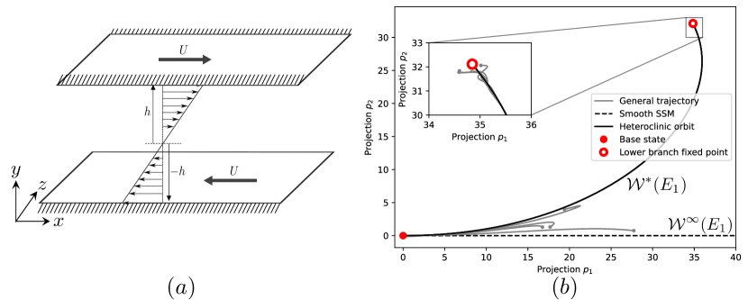
Figure 4: (a) The geometry of planar Couette flow. (b) Projection of the full Couette flow dynamics onto the first and second POD modes of the dynamics on the spectral subspace $E_{1}$ for $Re=134.52$. Solid red dot: stable base state; hollow red dot: unstable equilibrium state; black curve: 1D fractional SSM, $W^{*}\left(E_{1}\right)$ connecting the two steady states; dashed black line: primary (analytic) slow SSM $\mathcal{W^{\infty}}(E_{1})$ coinciding with $E_{1}$; grey curves: nearby trajectories converging to the base state.

As already mentioned in Section 2, Page and Kerswell [50] showed in detail the inevitable failure of linear model reduction methods to capture transitions among coexisting steady states in this flow. In contrast, Kaszás et al. [39] used data-driven SSM reduction to construct 1D and 2D models for such transitions. These models were obtained from an integer-powered polynomial approximation of the SSM. Here we will show that lower-order polynomial approximation to these manifolds are more accurate if we account for fractional-powered terms in the data-driven construction of the SSM.

The Navier–Stokes equations governing the evolution of the velocity field $\mathbf{u}(x,y,z,t)$ defined over the domain $(x,y,z)\in\Omega=[0,L_{x}]\times[-h,h]\times[0,L_{z}]$ can be written as

$$\frac{\partial\mathbf{u}}{\partial t}+(\mathbf{u}\nabla)\mathbf{u} =-\nabla p+\frac{1}{\text{Re}}\Delta\mathbf{u},$$ (60)

$$\nabla\cdot\mathbf{u} =0,$$

where $\mathrm{Re}=Uh/\nu$ denotes the Reynolds number with viscosity $\nu$ and $p$ is the pressure. To eliminate the pressure from (60), we recall the Helmholtz-decomposition to write $\mathbf{u}$ as

$$\mathbf{u}=\nabla\Phi+\mathbf{q},$$

where $\Phi$ is a scalar field and $\mathbf{q}$ is divergence free. The Leray projection of $\mathbf{u}$ , denoted by $\mathbb{P}[\mathbf{u}]$, extracts the divergence-free component of $\mathbf{u}$, i.e., returns $\mathbb{P}[\mathbf{u}]=\mathbf{q}.$ With this notation, the Leray projection of (60) becomes

$$\frac{\partial\mathbf{u}}{\partial t}=-\mathbb{P}\left[(\mathbf{u}\nabla)\mathbf{u}\right]+\frac{1}{\text{Re}}\Delta\mathbf{u}.$$ (61)

Denoting perturbations from the laminar solution $\mathbf{U}(y)=(y,0,0)$ by $\mathbf{v}$, we can rewrite the Leray-projected Navier-Stokes equation (61) as

$$\frac{\partial\mathbf{v}}{\partial t}=\frac{1}{\text{Re}}\Delta\mathbf{v}-\mathbb{P}\left[\left(\mathbf{U}\nabla\right)\mathbf{v}\right]-\mathbb{P}\left[\left(\mathbf{v}\nabla\right)\mathbf{U}\right]+\mathbb{P}\left[\left(\mathbf{v}\nabla\right)\mathbf{v}\right],$$ (62)

whose linear part,

$$\frac{\partial\mathbf{v}}{\partial t}=\frac{1}{\text{Re}}\Delta\mathbf{v}-\mathbb{P}\left[\left(\mathbf{U}\nabla\right)\mathbf{v}\right]-\mathbb{P}\left[\left(\mathbf{v}\nabla\right)\mathbf{U}\right],$$ (63)

is known as the Orr–Sommerfeld equation. Assuming periodicity in $x$ and $z$ allows us to expand $\mathbf{v}$ into Fourier-series as

$$\mathbf{v}(x,y,z,t)=\sum_{n,m}\mathbf{v}(y)e^{\lambda t}e^{i\alpha_{x}nx+i\alpha_{z}mz},$$

where the fundamental wave numbers are defined as $\alpha_{x}=\frac{2\pi}{L_{x}}$ and $\alpha_{z}=\frac{2\pi}{L_{z}}$. This turns the linearized equation (63) into an eigenvalue problem, with the eigenvalue denoted by $\lambda$. Using the explicit expressions of the differential operators involved (see, e.g., Schmid and Henningson [58]), one finds that the least stable mode is independent of $x$ and has eigenvalues and eigenfunctions of the form

$$\lambda_{1}=-\frac{\pi^{2}+4\alpha_{z}^{2}}{4\text{Re}}\qquad\mathbf{v}_{1}=\sin(\alpha_{z}z)\left(\begin{array}[]{c}\sin(\sqrt{\lambda_{1}\text{Re}}\,y)\\ 0\\ 0\end{array}\right).$$ (64)

For this mode, a direct calculation shows that

$$\mathbb{P}\left[\left(\mathbf{v}_{1}\nabla\right)\mathbf{v}_{1}\right]=\mathbf{0},$$

i.e., the nonlinear term in eq. (62) vanishes on the slowest eigenfunction. Consequently,

$$\mathcal{W^{\infty}}(E_{1})=E_{1}=\left\{\mathbf{U}(y)+\tau\mathbf{v}_{1}(y,z),\tau\in\mathbb{R}\right\}$$ (65)

is the primary, slow SSM of the laminar state.

Indeed, substituting an integer-powered polynomial expansion for an invariant manifold tangent to $E_{1}$ into the nonlinear equation (62) yields vanishing Taylor coefficients at all orders. In other words, such an expansion trivially converges and yields the single flat, analytic SSM shown as a dashed line in Fig. 4b. The dynamics on this primary SSM is governed by the linear system (63), and hence no connection from the laminar base state $\mathbf{U}(y)$ to any nontrivial steady state can be contained in $\mathcal{W^{\infty}}(E_{1})$. As a result, the transition to the base state to the other nontrivial steady state in system (62) must be a fractional SSM, $\mathcal{W}^{*}\left(E_{1}\right)$, anchored at the base state, just as in our simple example (1). We confirm this numerically in Fig. 4b, whose geometry bears a close similarity to that of our simple example in Fig. 1a.

The fractional SSM $\mathcal{W}^{*}\left(E_{1}\right)$ in Fig. 4b has limited differentiability. Yet a data-driven global approximation for this SSM still gives satisfactory results for high enough orders of regression, as shown by Kaszás et al. [39]. This is because every continuous curve can be arbitrarily closely approximated by smooth polynomials (Rudin [55]). The required order for such an approximation, however, is generally higher than necessary and leads to larger errors further away from the origin.

Here, we will seek the globally defined manifold $\mathcal{W}^{*}\left(E_{1}\right)$ in the asymptotic form (52) which has the same approximation power as polynomial expansions but also has the correct local form and correct degree of smoothness near the origin. We show that a data-driven fit of this exact fractional form for $\mathcal{W}^{*}\left(E_{1}\right)$ is indeed more accurate at a given order than the one with purely integer-powered polynomials.

We use Channelflow of Gibson et al. [30] with a spectral discretization of $n=\mathcal{O}\left(10^{5}\right)$ for the nonlinear system (62). For the parameter values chosen ($L_{x}=5\pi/2$, $L_{z}=4\pi/3$), we have $p=1$, $q=0$ and $r+s=n-1$ in terms of the notation used in Section 3. We use the discrete formulation of our results from Section 4 with an integer time sampling, which Kaszás et al. [39] found to give more robust reduced models than the continuous time formulation. The eigenvalues of the linearized map $\lambda_{\mathrm{map}}$ and the linearized flow $\lambda_{\text{flow}}$ at the base state are related to each other via $\lambda_{\mathrm{map}}=e^{\lambda_{\text{$\mathrm{flow}$}}}$ .

For these parameters, formulas (52) give the fractional SSM parametrization

$$v =\sum_{1\leq k_{1}+\sum_{\ell=1}^{r}k_{4\ell}\frac{\log\kappa_{\ell}}{\log\left|\lambda_{1}\right|}\leq\mathcal{K}}C_{\mathbf{k}}u_{1}^{k_{1}+\sum_{\ell=1}^{r}k_{4\ell}\frac{\log\kappa_{\ell}}{\log\left|\lambda_{1}\right|}}+o\left(\left|u_{1}\right|^{\mathcal{K}}\right),\qquad\mathbf{k}=\left(k_{1},\mathbf{k}_{2}\right)\in\mathbb{N}\times\mathbb{N}^{r},\quad C_{\mathbf{k}}\in\mathbb{R}^{n}.$$ (66)

In this expression, we have omitted the modulus of $u_{1}$ in the fractional powered terms as we are only interested in the positive branch of $\mathcal{W}^{*}\left(E_{1}\right)$ along which $u_{1}\geq 0$ can be chosen. A linear term with $\mathbf{k}=\left(1,\mathbf{0}\right)$ also appears in the expression (66) because the linear part of system (62) has not been diagonalized in the current set of coordinates.

The spectral ratio $\log\kappa_{1}/\log\lambda_{1}=1.989703$ in Table 1 shows that $\mathcal{W}^{*}\left(E_{1}\right)$ is only once continuously differentiable by formulas (50) if the coefficient $h_{\mathbf{k}}$ with $\mathbf{k}=\left(0,1,0,\ldots,0\right)$ is nonzero.

	value	$\frac{\log\kappa_{j}}{\log\left|\lambda_{1}\right|}$ (spectral ratio)
$\log\left|\lambda_{1}\right|$	-0.035068
$\log\kappa_{1}$	-0.069776	1.989703
$\log\kappa_{2}$	-0.073369	2.092178
$\log\kappa_{3}$	-0.140274	4.000013
$\log\kappa_{4}$	-0.168877	4.815674

Table 1: Leading eigenvalues of the base state in the plane Couette flow at $Re=134.52$ . The second column contains the first 5 eigenvalues, while in the third column we report the corresponding spectral ratios $\log\kappa_{j}/\log\left|\lambda_{1}\right|$.

Furthermore, Kaszás et al. [39] show that this heteroclinic connection between the base state is a graph over the square root of the energy input rate, $J=\sqrt{|I|},$ with the energy input rate

$$I[\mathbf{u}]=\frac{1}{2L_{x}L_{z}}\int_{0}^{L_{x}}\int_{0}^{L_{z}}\left(\left(\frac{\partial u}{\partial y}u\right)_{y=1}+\left(\frac{\partial u}{\partial y}u\right)_{y=-1}\right)\text{d}z\ \text{d}x-1.$$ (67)

Based on this, we will construct the fractional SSM $\mathcal{W}^{*}\left(E_{1}\right)$ as a graph over $J.$ Formally, this can be achieved by a change of coordinates. The observable $J$ is a function of the state,

$$J=F(x)=F(u_{1},...,u_{p},a,b,v,c,d),$$

where we recall the decomposition of (33). By the inverse function theorem, on a neighborhood of $x=0$, there exists a function $G$, such that $u_{1}=G(J,u_{2},...,u_{p},a,b,v,c,d)$, as long as

$$\left.\frac{\partial F}{\partial u_{1}}\right|_{x=0}\neq 0.$$

Let us now introduce the new state vector $\hat{x}=(J,\hat{u}_{2},...,\hat{u}_{p},\hat{a},\hat{b},\hat{v},\hat{c},\hat{d})$, which is related to $x$ through $x=g(\hat{x}),$ where

$$g(\hat{x})=\left(G(J,\hat{u}_{2},...,\hat{u}_{p},\hat{a},\hat{b},\hat{v},\hat{c},\hat{d}),\hat{u}_{2},\dots,\hat{u}_{p},\hat{a},\hat{b},\hat{v},\hat{c},\hat{d}\right)^{\mathrm{T}}.$$

Under this change of coordinates, (3) must be transformed as

$$\dot{\hat{x}} =(D_{\hat{x}}g)^{-1}\mathcal{A}(D_{\hat{x}}g)\hat{x}+\hat{f}(\hat{x}).$$ (68)

Since the linear part of (68) is related to the linear part of (3) through a similarity transformation, they have the same spectrum. This means, that we may view the manifolds as graphs over the variable $J$, and the parametrization contains the same fractional powers as the parametrization in the original phase space.

To compute $\mathcal{W}^{*}\left(E_{1}\right)$ up to order $5$ , we need to find all terms in (66) with integer and fractional powers up to $\mathcal{K}=5$. These powers satisfy

$$k_{1}+\sum_{\ell=1}^{\mathcal{K}-k_{1}}k_{4\ell}\frac{\log\kappa_{\ell}}{\log\left|\lambda_{1}\right|}\leq 5.$$

Since $\frac{\log\kappa_{5}}{\log|\lambda_{1}|}>5,$ we only have to use fractional terms arising from the eigenvalues with $\kappa_{1},...,\text{$\kappa_{4}$ in }$ (66). We also see from Table 1 that the fractional powers $\frac{\log\kappa_{j}}{\log\left|\lambda_{1}\right|}$ and $\frac{\log\kappa_{j}}{\log\left|\lambda_{1}\right|}$ are very close to the integer powers $2$ and $4$, which are also present in the expansion (66). While some of the near-integer spectral ratios arise due to resonances in the infinite-dimensional system, they are never exact resonances in the finite truncation of the system that we work with here. Nevertheless, to avoid sensitivity and overfit (see Remark 7), we set $k_{41}=k_{43}=0$. Based on these considerations, a quintic-order approximation for the SSM-reduced map $J(\imath)\mapsto J(\imath+1)$ can be written as

$$J(\imath+1)=\sum_{k_{1}+k_{42}\frac{\log\kappa_{2}}{\log\left|\lambda_{1}\right|}+k_{44}\frac{\log\kappa_{4}}{\log\left|\lambda_{1}\right|}\leq 5}R_{k_{1},k_{42},k_{45}}J(\imath)^{k_{1}+k_{42}\frac{\log\kappa_{2}}{\log|\lambda_{1}|}+k_{44}\frac{\log\kappa_{4}}{\log|\lambda_{1}|}}.$$ (69)

We determine the coefficients $R_{k_{1},k_{42},k_{44}}$ from linear regression by minimizing the squared error

$$\sum_{\imath=1}^{N_{s}}\left\|J(\imath+1)-\sum_{k_{1}+k_{42}\frac{\log\kappa_{2}}{\log\left|\lambda_{1}\right|}+k_{44}\frac{\log\kappa_{4}}{\log\left|\lambda_{1}\right|}\leq 5}R_{k_{1},k_{42},k_{45}}J(\imath)^{k_{1}+k_{42}\frac{\log\kappa_{2}}{\log|\lambda_{1}|}+k_{44}\frac{\log\kappa_{4}}{\log|\lambda_{1}|}}\right\|^{2},$$

along a training trajectory started on the heteroclinic orbit for the available data snapshots indexed by $\imath=1,\ldots,N_{s}$. This regression gives the coefficients listed in Table 2 for the reduced mapping (69):

$k_{1}$	$k_{42}$	$k_{44}$	$R_{k_{1},k_{42},k_{44}}$
1	0	0	0.96182
2	0	0	0.82616
0	1	0	-1.03809
3	0	0	0.43671
1	1	0	0.35338
2	1	0	-0.61552
4	0	0	-1.65568
0	2	0	0.67765
0	0	1	4.52449
5	0	0	-3.47146

Table 2: Coefficients $R_{k_{1},k_{42},k_{44}}$ in the reduced model (69) for transitions along the fractional SSM $W^{*}\left(E_{1}\right)$ in the planar Couette flow.

In Fig. 5, we compare the predictions of the model (69) with those of the model

$$J(\imath+1) =0.96262J(\imath)+0.04265J^{2}(\imath)-0.10282J^{3}(\imath)+0.24485J^{4}(\imath)-0.14738J^{5}(\imath),$$ (70)

which we obtain from a classical, integer-powered polynomial regression up to order $\mathcal{K}=5$. Note that this model is purely a numerical fit, given that the only SSM with an integer-powered expansion in the problem is $\mathcal{W}\left(E_{1}\right)=E_{1}$, whose expansion coefficients are all zero up to any order.

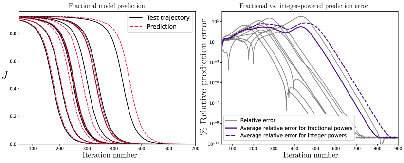
Figure 5: Performance of the fractional SSM-reduced model (69) for the planar Couette flow transition problem. Left: Reduced, 1D fractional model predictions (red) for 10 trajectories of the full system that were not used in regressing the model. Right: Instantaneous (gray) and mean errors (solid purple) for the fractional model and for a purely integer-powered fit (dashed purple) to the training trajectories. The relative error is defined as $|J_{true}(\imath)-J_{predicted}(\imath)|/\max J_{true}(\imath)$.

As seen from Fig. 5, there is a noticeable improvement in the correct, fractional expansion of the model relative to the formal, polynomial fit to the same data set up to the same order. The polynomial fit ignores five terms in the regression that do appear in the actual reduced dynamics below quintic order. The accuracy of the polynomial fit can only be increased by adding higher-order, integer-powered polynomials, which in turn add higher derivatives and hence more sensitivity to the model.

7 Example 2: Data-driven, mixed-mode, SSM-reduced model for the dynamic buckling of a beam

In our second example, we discuss the data-driven construction of a mixed-mode, SSM-reduced model for buckling using a discretized nonlinear von Kármán beam model. This model is a second-order approximation of geometrically exact beam theory that reproduces the bending-stretching coupling arising from bending displacements in the order of the beam thickness. We use the finite-element code of Jain et al. [37], who applied a combination of slow-fast reduction and SSM reduction to study oscillations of this beam model. In contrast, here we apply a sufficiently large longitudinal compression force and seek to derive an SSM-reduced nonlinear model for the ensuing buckling dynamics.

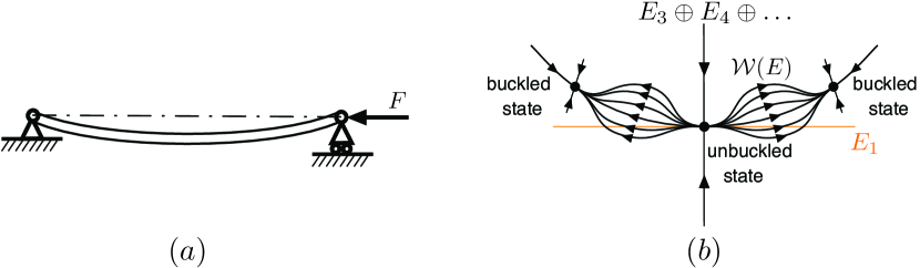
Figure 6: (a) Schematic of the geometry of the beam buckling under a horizontal force $F$. (b) Schematic of the family $\mathcal{W}\left(E\right)$ of 2D mixed-mode SSMs connecting the unstable unbuckled state to the two stable buckled states. The whole family $\mathcal{W}\left(E\right)$ is tangent to the unstable subspace $E_{1}$, as shown. However, only $\mathcal{W}^{\infty}(E)$ is tangent to the full spectral subspace $E$.

Schematically shown in Fig. 6, the finite element model of the von Kármán beam consists of $13$ nodes, each with three degrees of freedom (DOF): axial, transversal and rotational. By setting boundary conditions as pinned-pinned, we constrain 2 DOFs of the leftmost node and 1 DOF of the rightmost node. Therefore, the full system before model reduction has 12 elements and 72 DOFs. The beam is made of steel, with a Young’s modulus $E=1.9\cdot 10^{11}\,\mathrm{Pa}$, density $\rho=7,850\,kg/m^{3}$, viscous damping rate $\kappa=7\cdot 10^{6}\,kg\,m/s$, length $L=2\,m$, height $h=0,01\,m$ and width $w=0.05\,m$. Euler’s critical horizontal load for buckling is given by $P_{N}=N^{2}\pi^{2}EI/L^{2}$, with $I$ denoting the area moment of inertia of the cross section of the beam. Accordingly, to generate the first buckling mode ($N=1$), we apply the force

$$F=N^{2}\pi^{2}EI/L^{2}=\frac{1}{12}\pi^{2}Ebh^{3}/L^{2}.$$ (71)

.

7.1 2D primary mixed-mode SSM

Under the external force (71), the beam has three equilibria: one unstable equilibrium corresponding to purely axial displacement and two stable equilibria corresponding to the upper and lower buckled states. The first $10$ eigenvalues of the linearized finite element model at the unstable equilibrium are listed in Table 3, where we have already labelled the eigenvalues based on the role they will play in the construction of a mixed-mode SSM tangent to the 2D eigenspace

$$E=E_{1}\oplus E_{2},$$ (72)

with the 1D eigenspaces, $E_{1}$ and $E_{2}$ corresponding to the eigenvalues $\lambda_{1}=11.06$ and $\lambda_{2}=-11.10$, respectively. The remaining eigenvalues are all of the form $\beta_{m}\pm i\nu_{m}$ with $m>4$.

$\lambda_{1}$	$\lambda_{2}$	$\beta_{1}\pm i\nu_{1}$	$\beta_{2}\pm i\nu_{2}$	$\beta_{3}\pm i\nu_{3}$	$\beta_{4}\pm i\nu_{4}$
$11.06$	$-11.10$	$-0.36\pm i119.36$	$-1.83\pm i295.56$	$-5.80\pm i541.50$	$-14.19\pm i858.19$

Table 3: The first $10$ eigenvalues of the linearized finite-element model for a buckling beam at its unstable fixed point. Our notation is relative to the 2D eigenspace $E$ defined in (72).

To obtain a reduced model that captures the dynamics of buckling, we seek reduction to a member of the SSM family $\mathcal{W}\left(E\right)$. Therefore, we have $p=2$, $q=r=0$ and $s=n-2$ with $n=144$ in terms of the notation used in Theorem 1. By statement (ii) Theorem 1, a typical member of this mixed-mode family is only continuous, given that

$$\eta=\mathrm{Int}\left[\min_{j,k,\ell,m}^{+}\left\{\frac{\beta_{m}}{\lambda_{j}}\right\}\right]=\mathrm{Int}\left[\min_{m\geq 1}\left\{\frac{\beta_{m}}{\lambda_{2}}\right\}\right]=\mathrm{Int}\left[\frac{0.36}{11}\right]=0.$$

All these fractional SSMs and the primary SSM, $\mathcal{W}^{\infty}(E)$, contain all three fixed points and are all tangent to the 2D stable subspaces of the two buckled fixed points, as illustrated in Fig. 6b. For this reason, we select $\mathcal{W}^{\infty}(E)$ for constructing a reduced-order model because we can then use a classical polynomial expansion without fractional powers.

By Remark 1, the SSMLearn package of Cenedese et al. [18] can be used directly to approximate the primary mixed-mode SSM in this example. We use two training trajectories whose initial conditions are obtained via a positive and a negative vertical force applied to the midpoint of the beam, respectively. We then turn off the vertical forces and record the approach of the resulting two trajectories to the upper and lower buckled state of the beam. The two trajectories obtained in this fashion are shown in Fig. 7a, projected to a 3D coordinate space comprising the transverse displacement $q_{18}$ and velocity $\dot{q}_{18}$ of the midpoint, as well as the axial displacement $q_{35}$ of right endpoint. Figure 7b shows the primary mixed-mode SSM, $\mathcal{W}^{\infty}(E),$ projected onto the same coordinate system, along with truncated versions of the two training trajectories. Figure 7c shows truncated training trajectories in model coordinates from the spectral subspace $E=E_{1}\oplus E_{2}$. Finally, Figure 7d shows two truncated test trajectories of the full mechanical model system and predictions for them by the $\mathcal{W}^{\infty}(E)$-reduced and normalized 2D model.

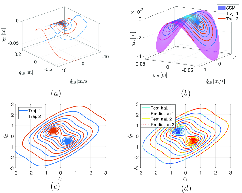
Figure 7: Construction and testing of a reduced model on the 2D, primary, mixed-mode SSM of the buckling beam problem. (a) Training trajectories. (b) The primary mixed-mode SSM, $\mathcal{W}^{\infty}(E)$, together with the two training trajectories. (c) Training trajectories in model coordinates. (d) Test trajectories of the full system along with model predictions for them.

Following the procedure outlined by Cenedese et al. [18] for data-driven primary SSMs, we find that both the invariance error of the manifold and the accuracy of the reduced-order model for the dynamics on the manifold is minimal at a polynomial order of $11$. This minimum, however, is quite weak for the invariance error and allows us to choose an order $\mathcal{K}=7$ approximation that reaches almost the same accuracy, resulting in a $0.1\%$ normalized error in fitting $\mathcal{W}^{\infty}(E)$ to the trajectories (see Cenedese et al. [18] on computing this error). Figure 7b shows the result of the data-driven identification of $\mathcal{W}^{\infty}(E)$ by SSMLearn, along with two training trajectories used in the procedure. Each training trajectory is truncated to a segment with no initial transients, which ensures that the trajectory is close to the SSM to be inferred from the data.

The training trajectories are also shown in Fig. 7c in modal coordinates that parametrize the spectral subspace $E.$ Finally, Fig. 7d shows a highly accurate prediction by the 2D $7^{th}$-order reduced model on $\mathcal{W}^{\infty}(E)$ for two test trajectories of the full system that were not used in the construction of the SSM-reduced model. We applied no normal form transformation to this model, because the two stable buckled states are far from the origin and hence are fully expected to lie outside the validity of a truncated normal form.

7.2 4D primary mixed-mode SSM

The reduced-order model derived in the previous section already captures the core dynamics (ie., all stable and unstable steady states) of the bucking beam.To illustrate how enlarging the dimension of the SSM reveals more transient behavior for larger initial conditions (see Remark 9), we repeat the above procedure for a 4D primary SSM constructed over the enlarged spectral subspace

$$E=E_{1}\oplus E_{2}\oplus E_{3}.$$ (73)

Here the newly added, 2D real eigenspace $E_{3}$ corresponds to the eigenvalue pair $-0.36\pm i119.36$ in Fig. 3. This means that we now have $p=2$, $q=1$, $r=0$ and $s=n-4$ with $n=144$ in the application of Theorem 1. Accordingly, our notation for the eigenvalues featured in the theorem changes from that in Fig. 3 to that in Table 4.

$\lambda_{1}$	$\lambda_{2}$	$\alpha_{1}\pm i\omega_{1}$	$\beta_{1}\pm i\nu_{1}$	$\beta_{2}\pm i\nu_{2}$	$\beta_{3}\pm i\nu_{3}$
$11.06$	$-11.10$	$-0.36\pm i119.36$	$-1.83\pm i295.56$	$-5.80\pm i541.50$	$-14.19\pm i858.19$

Table 4: Same eigenvalues as in Fig. 3, but now labelled with respect to the modified definition (73) of the spectral subspace $E$.

By Theorem 1, a typical fractional SSM in the $\mathcal{W}\left(E\right)$ family is still only continuous, given that

$$\eta=\mathrm{Int}\left[\min_{j,k,\ell,m}^{+}\left\{\frac{\beta_{m}}{\lambda_{j}},\quad\frac{\beta_{m}}{\alpha_{k}}\right\}\right]=\mathrm{Int}\left[\min_{m\geq 1}\left\{\frac{\beta_{m}}{\lambda_{2}},\frac{\beta_{m}}{\alpha_{1}}\right\}\right]=\mathrm{Int}\left[\frac{1.83}{11}\right]=0.$$ (74)

The geometry depicted in Fig. 6b remains similar for the choice of $E$ in (73) which again prompts us to choose the primary, mixed-mode SSM $\mathcal{W}^{\infty}\left(E\right)$ for reduced-order modeling. This SSM, however, is now 4D and hence cannot be easily visualized.

We initialize four new training trajectories in a way that they involve oscillations from the second buckling mode as well. To generate each training trajectory, we apply two vertical forces of opposing orientations at $1/4$ and $3/4$ of the total length of the beam to create a static, horizontal S-shaped equilibrium state for the beam. We then turn off these forces and use the resulting trajectories shown in Fig. 8a for extracting the 4D mixed-mode SSM $\mathcal{W}^{\infty}(E)$ and its reduced dynamics. Figures 8b-c show extended model prediction accuracy that now even capture transients of the test trajectories that were not used in constructing the model.

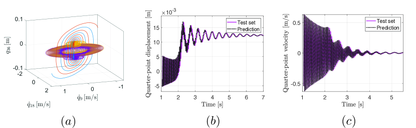
Figure 8: Construction and testing of a reduced model on the 4D, primary mixed-mode SSM of the buckling beam problem. (a) Four training trajectories projected to a 3D plane of the $\dot{q}_{18}$ transverse velocity of midpoint, the $\dot{q}_{9}$ transverse velocity of quarter-node and the $q_{36}$ rotation of the endpoint. (b) The quarter-node displacement of a test trajectory of the full beam model and a prediction for it by the $\mathcal{W}^{\infty}(E)$-reduced and normalized 4D model. (c) Same as (b) but for the quarter-node velocity of a test trajectory.

We close by recalling that within mixed-mode SSMs families, just as within like-mode SSMs, there are primary and secondary (fractional) SSMs. For instance, the SSMs computed in Sections 7.1 and 7.2 are primary mixed-mode SSMs. They also have fractional mixed-mode counterparts, which we did not have to compute in this case because of the manifold geometry shown in Fig. 6b.

8 Example 3: Fractional and mixed-mode SSMs in a forced oscillator system

Our third example involves a forced version of the 2 DOF nonlinear oscillator system originally proposed by Shaw and Pierre [60], which has been widely used to illustrate the concept of nonlinear normal modes in mechanical systems. A forced and slightly modified version of this example shown in Fig. 9 was considered by Ponsioen et al. [52] with small forcing amplitudes for SSM-based model reduction. That system comprises two identical rigid bodies of mass $m>0$ that move horizontally without friction, with their positions marked by the coordinates $q_{1}$ and $q_{2}$. The bodies are connected to each other and two walls via identical springs of linear stiffness $k>0$. The first spring also has a softening cubic nonlinearity with coefficient $\gamma>0$, while the other two springs are subject to linear damping with coefficient $c>0$. The first body is subjected to external forcing of amplitude $A$ and frequency $\Omega$.

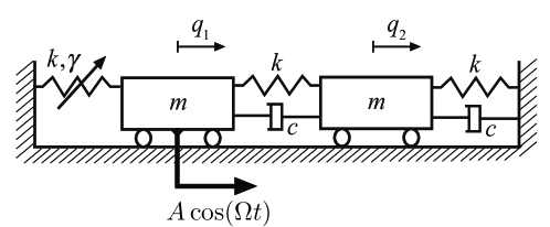
Figure 9: The periodically forced Shaw–Pierre oscillator from Ponsioen et al. [52].

With the notation $p_{1}=\dot{q}_{1}$, $p_{2}=\dot{q}_{2}$ , the first-order form of the equations of motion for the system is

$$\left(\begin{array}[]{c}\dot{q_{1}}\\ \dot{p}_{1}\\ \dot{q_{2}}\\ \dot{p_{2}}\end{array}\right)=\left(\begin{array}[]{cccc}0&1&0&0\\ -2\frac{k}{m}&-\frac{c}{m}&\frac{k}{m}&\frac{c}{m}\\ 0&0&0&1\\ \frac{k}{m}&\frac{c}{m}&-2\frac{k}{m}&-2\frac{c}{m}\end{array}\right)\left(\begin{array}[]{c}q_{1}\\ p_{1}\\ q_{2}\\ p_{2}\end{array}\right)+\left(\begin{array}[]{c}0\\ A\cos\Omega t-\frac{\gamma}{m}q_{1}^{3}\\ 0\\ 0\end{array}\right).$$ (75)

We first identify fractional SSMs near the trivial equilibrium of this system in the absence of external forcing $(A=0$). As a next step, under the addition of external time-periodic forcing ($A>0$), we construct a data-driven reduced model on a primary mixed-mode SSM of an unstable periodic orbit to capture transitions between coexisting periodic orbits. This second part of the example, therefore, serves as an illustration of our mixed-mode SSM results for discrete dynamical systems.

8.1 Fractional SSMs in the unforced Shaw–Pierre example ($A=0$)

Following Shaw and Pierre [60] and Ponsioen et al. [51], we fix the non-dimensionalized parameter values $m=1,$ $c=0.3,k=1,\gamma=0.5$. In that case, the eigenvalues of the linearized system near the origin are

$$\alpha\pm i\omega=-0.0741\pm 1.0027i\quad\beta\pm i\nu=-0.3759\pm 1.6812i,$$ (76)

where we have already applied the notation of Theorem 1 to the 2D spectral subspace $E$ corresponding to the slower decaying pair of complex eigenvalues. Then, after a linear change of coordinates, system (75) with $A=0$ will take the form

$$\left(\begin{array}[]{c}\dot{a}\\ \dot{b}\\ \dot{c}\\ \dot{d}\end{array}\right)=\left(\begin{array}[]{cccc}\alpha&\omega&0&0\\ -\omega&\alpha&0&0\\ 0&0&\beta&\nu\\ 0&0&-\nu&\beta\end{array}\right)\left(\begin{array}[]{c}a\\ b\\ c\\ d\end{array}\right)+f(a,b,c,d).$$ (77)

This system is of the general form (3) with $j=0$, $k=1$, $\ell=0$ and $m=1$. Therefore, formula (LABEL:eq:complex_SSM_1) simplifies to the single complex function

$$\mathcal{\mathcal{E}}(z) =Q\left|z\right|^{\frac{\beta}{\alpha}}e^{i\frac{\nu}{\alpha}\log\left|z\right|},$$

where $Q\in\mathbb{C}$ is a complex parameter.

In terms of the real $(a,b,c,d)$ coordinates, the full family of 2D invariant graphs of the linear part over the $E$ spectral subspace take the form

$$\left(\begin{array}[]{c}c(a,b)\\ d(a,b)\end{array}\right)=P_{1}\left(a^{2}+b^{2}\right)^{\frac{\beta}{2\alpha}}\left(\begin{array}[]{c}\cos\left(P_{2}+\frac{\nu}{2\alpha}\log\left[a^{2}+b^{2}\right]\right)\\ \sin\left(P_{2}+\frac{\nu}{2\alpha}\log\left[a^{2}+b^{2}\right]\right)\end{array}\right),\quad P_{1}=\left|Q\right|,\quad P_{2}=\arg Q,$$ (78)

which defines a two-parameter-family of invariant graphs in the linearized system, parametrized by $P_{1},P_{2}\in\mathbb{R}$.

As guaranteed by statement (i) of Theorem 1, the corresponding 2D, slow SSM family $\mathcal{W}\left(E\right)$ in the full nonlinear system (77) can be written near the origin as

$$w =\mathcal{\mathcal{E}}(z)+\sum_{2\leq k_{1}+k_{2}+\frac{\left(k_{3}+k_{4}\right)\beta}{2\alpha}\leq\mathcal{K}}h_{\mathbf{k}}z^{k_{2}}\bar{z}^{k_{3}}\mathcal{\mathcal{E}}^{k_{5}}\bar{\mathcal{\mathcal{E}}}^{k_{6}}+o\left(\left|z\right|^{\mathcal{K}}\right),\qquad\mathbf{k}=\left(k_{2},k_{3},k_{5},k_{6}\right).$$ (79)

By the complexification formula (14), when truncated at order $\mathcal{K}$ and re-indexed, this SSM family can be written in real coordinates as

$$\left(\begin{array}[]{c}c\\ d\end{array}\right) =\sum_{2\leq k_{1}+k_{2}+\frac{\left(k_{3}+k_{4}\right)\beta}{2\alpha}\leq\mathcal{K}}P_{1}^{k_{3}+k_{4}}\left(\begin{array}[]{c}C_{\mathbf{k}}\\ D_{\mathbf{k}}\end{array}\right)a^{k_{1}}b^{k_{2}}\left(a^{2}+b^{2}\right)^{\frac{\beta\left(k_{3}+k_{4}\right)}{2\alpha}}\times$$ (84)

$$\,\,\,\,\,\,\,\,\,\,\,\,\,\,\,\,\times\cos^{k_{3}}\left(P_{2}+\frac{\nu}{2\alpha}\log\left[a^{2}+b^{2}\right]\right)\sin^{k_{4}}\left(P_{2}+\frac{\nu}{2\alpha}\log\left[a^{2}+b^{2}\right]\right),$$ (85)

where

$$C_{0010}=D_{0001}=1,$$

and all other $C_{\mathbf{k}}$ and $D_{\mathbf{k}}$ coefficients with $\left|\mathbf{k}\right|=1$ are zero.

In all nonlinear normal mode and SSM calculations available in the literature for this model, only the $k_{3}=k_{4}=0$ terms of the above expansion have been used and hence only the unique primary SSM, $W^{\infty}\left(E\right)$, has been exploited for reduced-order modeling. This restriction to $W^{\infty}\left(E\right)$ is fully justified when $\beta/\alpha$ is relatively large ( $\beta/\alpha>\mathcal{K}$), in which case the fractional terms do not yet appear in the truncated expansion (85). For the parameter configuration used by Shaw and Pierre [60] and Ponsioen et al. [51], the eigenvalues in (76) give

$$\frac{\beta}{\alpha}=5.0729,$$

which means that fractional powers only appear in the expansion for any member of the $\mathcal{W}\left(E\right)$ family for orders $\mathcal{K}>5$. The $6^{th}$ order Taylor coefficients happen to vanish in this case, but the fractional coefficient $\sqrt{a^{2}+b^{2}}^{5.0729\left(k_{3}+k_{4}\right)}$ does appear and starts shaping the secondary SSMs and their reduced dynamics already below order $6$.

To show the difference between the primary SSM $W^{\infty}\left(E\right)$ and the secondary (fractional) SSMs in the full SSM family (85), we explicitly calculate the Taylor expansion of the $C^{\infty}$ linearizing transformation underlying the results of Theorem 1 for the present model up to and including order 7. In Fig. 10 we show the transformed images of some of the SSMs of the linearized system (78) under the inverse of that linearizing transformation. Note the difference between the smooth $W^{\infty}\left(E\right)$ ($P=0$, $Q=0$ in (78)) and the general fractional SSMs, which arises because fractional terms do start appearing beyond order $\mathcal{K}=6$. The figure also shows a general, decaying trajectory that follows the fractional SSM and only approaches $W^{\infty}\left(E\right)$ closer to the origin.

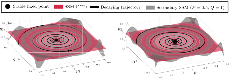
Figure 10: Primary and fractional slow SSMs in the unforced ($A=0$) limit of the Shaw-Pierre model (75). The $q_{1}$ and $p_{1}$ coordinates of the slow SSMs are plotted in panels (a) and (b), respectively. Red surface: order $K=7$ approximation of the analytic SSM $W^{\infty}\left(E\right)$. Grey surface: fractional SSM of order $\mathcal{K}=7$ with $P=0.5$ and $Q=1$. Black curve: a general, decaying trajectory off the primary SSM.

8.2 Mixed-mode SSM of a periodic orbit in the forced Shaw–Pierre example ($A>0$)

Let us now consider system (75) with a lower value of damping, $c=0.03$, as in [52] for which the forced response curves of the model are given in Fig. 11 for several forcing amplitudes $A$. Also shown are the theoretically computed backbone curves from SSMTool (see Jain and Haller [36]), which are based on a leading-order approximation to the time-periodic perturbation of $W^{\infty}\left(E\right)$. Note that for larger forcing amplitudes with $A>0.085$, even the $\mathcal{O}\left(15\right)$ theoretical predictions based on $W^{\infty}\left(E\right)$ divert from the actual periodic response.

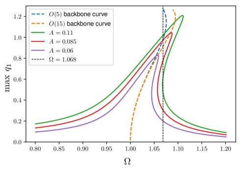
Figure 11: Forced response curves (i.e., maximal amplitudes of the observed steady-state oscillations of the first mass as a function of the forcing frequency $\Omega$) of the Shaw-Pierre system for different forcing amplitudes $A$. Dashed lines represent the backbone curves (i.e., theoretical centerpieces of the forced response curves) predicted by SSMTool from a reduced-order model on the analytic slow SSM.

To improve on these predictions, we focus on the forcing frequency $\Omega=1.07$ and forcing amplitude $A=0.11$ for which 3 periodic orbits coexist: a high-amplitude stable periodic orbit, a saddle-type periodic orbit and a low-amplitude stable periodic orbit. Their stability types can be more specifically determined by computing their Floquet multipliers numerically, which we show in Fig. 12. For our analysis, the most important is the spectrum of the saddle-type periodic orbit. With the notation used in Theorem 2, the Floquet-multipliers of that periodic orbits are $\lambda_{1},\lambda_{2}$ and $\beta\pm i\nu$, where

$$\lambda_{1} =1.0835,\quad\lambda_{2}=0.7726,\quad\beta=-0.4132,\quad\nu=0.6474.$$

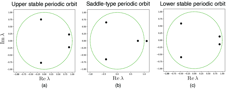
Figure 12: Panels (a)-(c) show, for $\Omega=1.07$ $A=0.11$, the Floquet multipliers of the upper periodic orbit, the saddle-type periodic orbit in the middle, and the lower periodic orbit, respectively. The green dashed line represents the unit circle.

To explore transitions among the coexisting periodic orbits, we consider the time-$T$ Poincaré map associated with the forced system (75). All three periodic orbits have period $T$ and hence all are hyperbolic fixed points of this map, as seen from their Floquet multipliers in Fig. 12. To capture connections among the fixed points, we seek to construct the 2D mixed-mode SSM family tangent to the 2D spectral subspace $E$ that is spanned by the stable and unstable real eigenvectors of the saddle points. Of these mixed-mode SSMs, we only consider the primary one, $\mathcal{W^{\infty}}\left(E\right)$, for the same reason as in the beam buckling problem (see Fig. 6b). The existence and uniqueness of this $\mathcal{W^{\infty}}\left(E\right)$ follows from statement (iii) of Theorem 2, given that the Floquet multipliers of the saddle fixed point are nonresonant.

Since the Poincaré map is not known explicitly, we have no direct access to the quantities featured in Section 3 for the map formulation of our main results. For a data-driven construction, we launch four trajectories along the tangent space with initial conditions

$$x_{0}^{(1,2,3,4)}=x_{0}\pm\delta\mathbf{e}_{1}\pm\delta\mathbf{e}_{2},$$

where $x_{0}$ is the location of the saddle-type fixed point, $\mathbf{e}_{1}$ is its unstable eigenvector, $\mathbf{e}_{2}$ is its weakest stable eigenvector, and $\delta=0.01.$ We use these trajectories for extracting the primary mixed-mode SSM $\mathcal{W^{\infty}}\left(E\right)$ via polynomial regression. In Fig. 13, we show the iterates of the four training trajectories under the time-$T$ map of system (75) via a projection onto the $(q_{1},p_{1})$ coordinate plane.

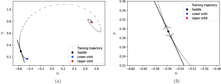
Figure 13: Training trajectories for constructing the 2D primary, mixed-mode SSM, $\mathcal{W^{\infty}}\left(E\right)$, of the Poincaré map of the Shaw–Pierre model (75). (a) Iterates of the four training initial conditions initialized near the saddle-type fixed point. The unstable eigenvector $\mathbf{e}_{1}$ is shown with the black vertical line. (b) Magnification of the region around the saddle.

To illustrate the accuracy of this reduced-order model on $\mathcal{W^{\infty}}\left(E\right)$, we generate $20$ test trajectories that are initialized near the saddle. Each initial condition has a distance of $2\cdot 10^{-2}$ from the saddle point. Figure 14 shows that these test trajectories indeed closely track the extracted $\mathcal{W^{\infty}}\left(E\right)$ in a 3D projection from the 4D phase space of the Poincaré map.

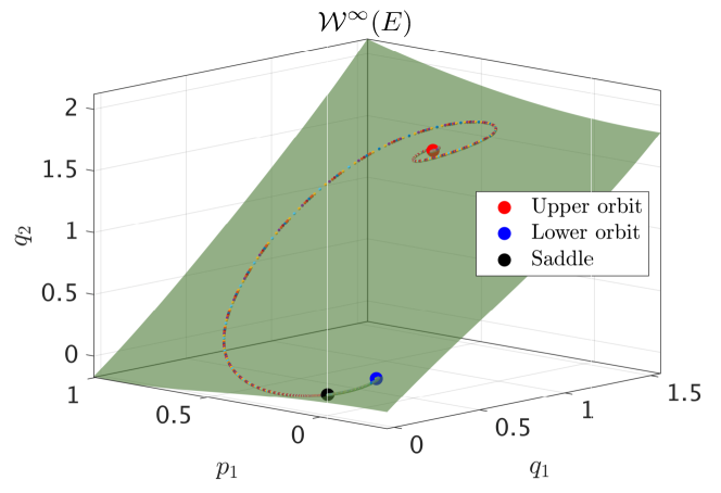
Figure 14: Fixed points and test trajectories on the primary, mixed-mode SSM, $\mathcal{W^{\infty}}\left(E\right)$, of the Poincaré map of the Shaw–Pierre model (75). The test trajectories are initialized near the saddle point and their iterates are denoted by colored dots. The extracted SSM is the green surface.

We can also make predictions for the time evolution of these test trajectories using solely the reduced discrete model. The resulting trajectories obtained from the iterations of the full Poincaré map and the predictions for them using the 2D reduced dynamics match closely, as seen in Fig. 15.

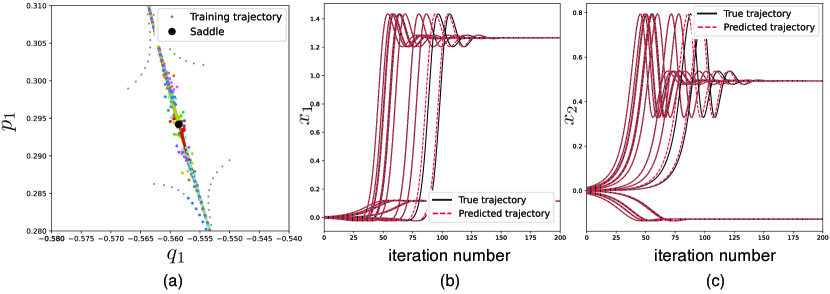
Figure 15: Test trajectories of the full Poincaré map and their corresponding predictions from the 2D reduced model on $\mathcal{W^{\infty}}\left(E\right)$ for the Shaw–Pierre model (75). (a) Test trajectories shown as colored dots, initialized near the saddle-type fixed point of the map. (b)-(c) Evolution of $q_{1}$ and $p_{1}$, respectively, along with the predictions of the $5^{th}$-order $\mathcal{W^{\infty}}\left(E\right)$-reduced model. The discrete iterates are connected into continuous lines for visual clarity.

9 Conclusions

We have extended the existing theory of (primary, or smoothest) spectral submanifolds to the full family of continuous invariant manifolds that emanate from a nonresonant fixed point of a generic finite-dimensional, class $C^{\infty}$ continuous or discrete dynamical system. This extended family now includes nonlinear continuations of spectral subspaces of mixed stability type and/or of finite smoothness. For the latter type of manifolds (fractional SSMs), we have derived a formal expansion with specific fractional powers that can be inferred from the spectrum of the linearized system. We have obtained similar results for discrete dynamical systems defined by iterated mappings. We have illustrated our results both for discrete and continuous dynamical systems on the data-driven reduced-order modeling of non-linearizable behavior in three physical systems: a canonical shear flow, a buckling beam and a forced nonlinear rigid body system.

The main technical tool we rely on to prove these results is a classic linearization result of Sternberg [63], coupled with the explicit construction of all continuous invariant manifolds through the origin of a general, multi-dimensional linear system with a hyperbolic fixed point. Neither this linearization result nor its refinements (see, e.g. Sell [59]) are specific enough about the smoothness of the linearizing transformation, except for the class of $C^{\infty}$ dynamical systems considered here, for which the linearization is also of class $C^{\infty}$. We note that the linearizing transformation only converges on a domain around the fixed point in which the original system exhibits linearizable behavior, completely missing all interesting dynamical phenomena that arise from the coexistence of several isolates invariant sets. For this reason, we do not advocate linearization for model reduction and only use linearization here to identify the function basis over which an SSMs should be more globally approximated from data. Specifically, we use truncated, finite fractional expansions for the SSMs and its reduced dynamics in our three data-driven examples. These truncated expansions continue to be well-defined outside the domain of linearizable behavior as well and hence have the potential to capture nontrivial dynamics, as we illustrate on examples.

A conceptual limitation of the results in this paper is that it assumes the underlying dynamical system to be finite dimensional. This is not an issue for numerical data sets or solid or fluid mechanics, as those are always generated from finite-dimensional discretization of their originally infinite-dimensional governing equations. Nevertheless, for experimental data obtained from a physical system, it would be desirable to have a general, infinite-dimensional extension of Sternberg’s linearization results that we use. Such an extension is available for the most frequent case in practice, wherein the spectrum of the linearized system is either fully in the left-hand or the right-hand side of the complex plane, i.e., satisfies the conditions of statement (v) in Theorems 1 or 2 (see Elbialy [24]). This extension implies that the finite-dimensional like-mode, primary and fractional SSMs we have identified have infinite-dimensional limits under appropriate spectral gap conditions. As for primary mixed-mode SSMs, their existence and uniqueness in infinite dimensions has been known under appropriate spectral gap conditions as long as they are also pseudo-unstable or pseudo-stable manifolds, i.e., normally hyperbolic and purely repelling or purely attracting, respectively (Elbialy [25]). Primary pseudo-stable manifold SSMs, which also include primary like-mode SSMs, have also been proven to exist by Buza [12] specifically for the Navier–Stokes equations.

A more practical challenge for the fully data-driven application of our results is that the fractional powers in the parametrization of secondary SSMs depend on the real part of the spectrum of the linearization outside the underlying spectral subspace $E$. While traces of frequencies outside of $E$ can be extracted from the frequency analysis of the available data, the real parts of the eigenvalues are more difficult to identify. An option is to treat the leading-order fractional powers as unknowns and determine them from a maximum likelihood regression. This approach shows promise in some of our preliminary numerical tests, but may also identify physically incorrect values for the fractional powers in some other examples we have considered. Another option is to estimate the real parts of the dominant eigenvalues outside $E$ from a linear data-driven method, such as DMD or EDMD. A third option is to excite individual modes at small amplitudes and infer their decay rates by fitting one-degree-of-freedom linear oscillators to their forced response curves. The detailed implementation of these strategies will be pursued in other publications.

The backbone curves and damping curves derived in Section 4 from a fractional normal form should be helpful in explaining some unexpected backbone curves and instantaneous damping curves observed in detailed experimental data from gravity measurements and hydrogel oscillations (Cenedese [15], Eriten [26]). In those experiments, the observed shapes of backbone curves and instantaneous damping curves cannot be explained without including the fractional-powered terms in formulas (58) and (58), which provided the original motivation of our present study. These experimental data sets along with others will be analyzed elsewhere with the methods developed here.

We close by noting that the fractional polynomial powers identified in Theorems 1 and 2 generically arise in the reduced dynamics of any non-unique invariant manifold emanating from hyperbolic fixed points. This implies that even other data-driven modeling approaches ignoring the existence of SSMs (e.g., EDMD and SINDy) would benefit from including such fractional powers in the dictionary of functions that they seek to fit to data.

10 Supplementary Material

In this section, we give technical details for Example 1 (Appendix A) and Example 2 (Appendix B). We also prove Theorem 1 (Appendix C), Propositions 1 and 2 (Appendix D), Theorem 2 (Appendix E), Propositions 3 and 4 (Appendix F), and Theorem 3 (Appendix G).

ACKNOWLEDGMENT

We acknowledge helpful discussion with Mattia Cenedese and Melih Eriten. We are also grateful to Gergely Buza for bringing Ref. [12] to our attention.

AUTHOR DECLARATIONS

Conflict of Interest

The authors have no conflicts to disclose.

Author Contributions

George Haller: Conceptualization (lead), Methodology (lead), Formal analysis (lead), Supervision (lead), Writing – original draft (lead). Bálint Kaszás: Conceptualization (equal), Formal analysis (lead), Data Curation (equal), Writing – original draft (equal), Writing – review & editing (equal). Aihiu Liu: Conceptualization (equal); Formal analysis (equal), Data Curation (equal), Writing – original draft (equal); Joar Axås: Conceptualization (equal), Supervision (equal), Writing – review & editing (equal).

DATA AVAILABILITY

All code and data used in the paper will be made available upon publication under https://github.com/haller-group.

Supplementary Material

11 Appendix A: Details for example (1)

11.1 Explicit solutions

We seek invariant manifolds of system

$$\dot{x} =x(y-b),$$

$$\dot{y} =cy(x-a),$$ (86)

with the parameters $a,b,c>0$ that can be written as

$$W(E_{1})=\{(x,h(x)):x\in\mathbb{R}\}.$$

Substituting $y=h(x)$ into the differential equation we get the invariance equation

$$x\left(h(x)-b\right)\frac{d}{dx}h(x)=ch(x)\left(x-a\right).$$ (87)

A solution to (87) is $h(x)=0$, which is the analytic smooth SSM, as we will see later. Assuming that $h(x)\neq 0$, we may rearrange (87) to obtain

$$\frac{c(x-a)}{x}=\frac{h^{\prime}(x)[h(x)-b]}{h(x)},$$

where differentiation with respect to $x$ is denoted by a prime. We may integrate both sides of this equation, after which we have

$$c(x-a\log x)=h(x)-b\log h(x)+C,$$

for some $C\in\mathbb{R}$, a constant of integration. This is an algebraic relationship, which already gives an implicit definition for the manifold $y=h(x).$ However, we may rearrange this to search for an explicit expression. With the substitution $\hat{h}=-\frac{h(x)}{b},$ we can obtain

$$-\frac{1}{b}e^{-\frac{cx}{b}+\frac{C}{b}}x^{\frac{ca}{b}}=e^{\hat{h}}\hat{h}(x).$$ (88)

Note that the solution $h(x)\equiv 0$ is a singular solution of (87), because it cannot be obtained from (88) for any choice of the parameter $C$: for $x\neq 0$, the left-hand side is never zero, which means $h\neq 0$. The implicit relation (88) can be solved for $h(x)$ using the Lambert $W$ function, which is also called the product logarithm function (see, e.g., Bronshtein and Semendyaev [8]). This is defined through the inverse relation

$$z=we^{w},$$

which can be solved for $w$ if $z\geq-\frac{1}{e}$. In this case, the solution is $w=W_{m}(z)$ for $m=-1$ or $m=0$, denoting the two branches of the $W$ function. This allows us to express the family of invariant manifolds, parametrized by the constant of integration $C$, as

$$h(x)=-bW_{m}\left(-\frac{1}{b}e^{-\frac{cx}{b}+\frac{C}{b}}x^{\frac{ca}{b}}\right).$$ (89)

To decide which branch of the $W$ function we need, we note that at $x=0$, the $m=-1$ branch diverges. The $m=0$ branch on the other hand is well defined at $x=0$ for all values of $C$. Since we are interested in an invariant manifold that contains the fixed point at the origin, we will use the principal branch $W_{0}$ of the $W$ function.

We can also determine the value of the constant $C$, if we require $h(x)$ to also contain the fixed point at $(a,b)$. The relationship $h(a)=b$ implies

$$W_{0}\left(-\frac{1}{b}e^{-\frac{ca}{b}+\frac{C^{*}}{b}}a^{\frac{ca}{b}}\right)=-1,$$

which can be solved for $C^{*}$ as

$$C^{*}=b\log\left(\frac{b}{e}a^{-\frac{ca}{b}}\right)+\frac{ca}{b},$$

to arrive at the particular member of the family of the invariant manifolds that contains both fixed points of system (86). This finally gives the exact reduced order model

$$\dot{x}=-bx\left[W_{0}\left(-\frac{1}{b}e^{-\frac{cx}{b}+\frac{C^{*}}{b}}x^{\frac{ca}{b}}\right)-1\right]$$

on the attracting SSM that connects the two fixed points.

11.2 POD, DMD and Koopman decompositions

One can consider the proper orthogonal decomposition (POD) on this problem to see if a projection to the dominant POD mode yields good reduced-order dynamics. If POD yields a dominant POD mode along a yet unknown line $y=Kx,$ then projection of the right-hand side of (86) to this line gives the equation

$$=\left.\frac{\left(x(y-b),cy(x-a)\right)\cdot\left(1,K\right)}{\sqrt{K^{2}+1}}\right|_{y=Kx}=\left.\frac{\left(x(Kx-b),cKx(x-a)\right)\cdot\left(1,K\right)}{\sqrt{K^{2}+1}}\right|_{y=Kx}$$ (90)

$$=\frac{K+cK^{2}}{\sqrt{K^{2}+1}}x\left[x-\frac{b+cK^{2}a}{K+cK^{2}}\right].$$

On the other hand, projecting the left-hand-side of (86) results in

$$\left.\frac{\left(\dot{x},\dot{y}\right)\cdot\left(1,K\right)}{\sqrt{K^{2}+1}}\right|_{y=Kx}=\left.\frac{\dot{x}+K\dot{y}}{\sqrt{K^{2}+1}}\right|_{y=Kx}.$$ (91)

Equating (91) and (90), we obtain the POD-based model

$$\dot{x}=\frac{K+cK^{2}}{1+K^{2}}x\left[x-\frac{b+cK^{2}a}{K+cK^{2}}\right].$$ (92)

This POD model will always have a fixed point at the origin and at another location, which is not necessarily $x=b$. Figure 16 shows the results of POD-based reduced order modeling for example (86) with $a=b=1$ and $c=2.5$. The model is not accurate for the details of the transition orbit but has the correct asymptotic behavior in forward time. Note, however, that deriving this reduced-order model required the knowledge of the full set of equations of the dynamical system, and hence this approach is inapplicable in a data-driven setting.

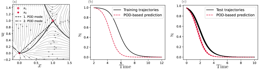
Figure 16: POD-based reduced order model example (86). Panel (a) shows the phase space of system (86) along with the numerically computed POD modes (dashed lines). The slope of the first POD mode is $K=0.95764$. In panels (b) and (c) the predicted dynamics is compared with the true dynamics for training and testing trajectories, respectively.

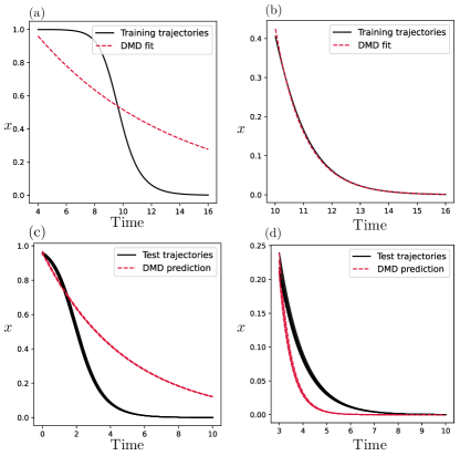
Figure 17: DMD-based reduced order models. (a) DMD fit to a full transition trajectory. (b) DMD fit to a subset of the same transition trajectory closer to the origin. (c) Predictions (red) from the DMD fit in (a) for test trajectories of the full system. (d) Predictions (red) from the DMD fit in (b) for truncated test trajectories of the full system.

Dynamic mode decomposition (DMD) is fully data driven and will fit a linear dynamical system to trajectories. This system will clearly have a stable node for small amplitude training data and a saddle for larger-amplitude training data. Figure 17 illustrates the prediction quality of two different DMD models: one fitted to the full transition trajectory (Fig. 17a) and one fitted to a truncated subset of the transition trajectory closer to the origin (Fig. 17b). The second fit can capture the asymptotic behavior (see the decay to the origin in Fig. 17d) but neither fit can make reliable predictions outside a small neighborhood of the origin, as expected.

A numerically constructed Koopman decomposition will behave similarly, given that it can only capture linearizable dynamics. Theoretically, the two $C^{1}$-unique principal Koopman eigenfunctions (see Kvalheim and Revzen [41]) associated with the domain of attraction of the origin are necessarily the ones whose zero set is the $x$ axis. On this, the dynamics is indeed globally linear and hence does not capture the nontrivial fixed point and the heteroclinic connection of interest.

11.3 Reduced-order models on fractional SSMs

By Theorem 1 of the main text, there exist a family $\mathcal{W}\left(E\right)$ of continuous SSMs tangent to the spectral subspace $E=\left\{\left(x,y\right)\in\mathbb{R}^{2}:\,y=0\right\}$ in example (86). By Proposition 1, for an arbitrary integer $\mathcal{K}\geq 2$, the $x\geq 0$ branches of members of this family can be written as

$$y =C_{\left(0,1\right)}(x)x^{\frac{k_{4}ac}{b}}+\sum_{2\leq k_{1}+k_{4}\frac{ac}{b}\leq\mathcal{K}}C_{\mathbf{k}}(x)x^{k_{1}+k_{4}\frac{ac}{b}}+o\left(\left|x\right|^{\mathcal{K}}\right),\qquad\mathbf{k}=\left(k_{1},k_{4}\right),$$ (93)

with the arbitrary, piecewise constant functions $C_{\mathbf{k}}(x)\in\mathbb{R}$ satisfying

$$C_{\mathbf{k}}(x)=\left\{\begin{array}[]{c}C_{\mathbf{k}}^{+}\qquad x>0,\\ \\ C_{\mathbf{k}}^{-}\qquad x\leq 0.\end{array}\right.$$

Restriction of example (86) to this invariant family of graphs gives the reduced-order model family

$$\dot{x}=x\left[-b+C_{\left(0,1\right)}\left|x\right|^{k_{4}\frac{ac}{b}}+\sum_{2\leq k_{1}+k_{4}\frac{ac}{b}\leq\mathcal{K}}C_{\mathbf{k}}(x)\left|x\right|^{k_{1}+k_{4}\frac{ac}{b}}+o\left(\left|x\right|^{\mathcal{K}}\right)\right].$$ (94)

One member of this family is the primary SSM $\mathcal{W}^{\infty}\left(E\right)=E$ satisfying $C_{\mathbf{k}}=0$ for all $\mathbf{k}$. Another member is the heteroclinic connection $\mathcal{W}^{*}\left(E\right)$ that is generally of class $C^{\mathrm{Int\left[ac/b\right]}}$ smooth. In the data-driven setting, the parameters in the formulas (93)-(94) can be determined by regression to training trajectories that are in a neighborhood of the heteroclinic orbit.

For comparison with the POD and DMD-based reduced-order models, we show the predictions obtained by a data-driven reduced-order model for example (86). In particular, using a single trajectory initialized close to the heteroclinic orbit, we compute the fractional SSM (93) up to order $\mathcal{K}=5$ via regression. Restricting to this fractional SSM then yields the reduced-order model (94) with specific coefficients up to order $\mathcal{K}=5$ . Figure 18 shows the close agreement between the predicted and true time evolutions of 5 test trajectories initialized close to the saddle. We also show the close agreement with the exact, analytically obtained reduced-order model, as well as the substantially larger errors produced by DMD and POD.

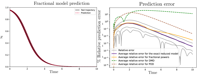
Figure 18: Fractional SSM-based reduced-order model compared with other model reduction methods for example (1). In the left panel we show the time evolution of 5 test trajectories along with the predicted time evolution based on the 5th order model. In the right panel, we show the prediction errors from data-driven fractional SSM reduction (yellow), DMD (green) and POD reduction (brown). For comparison, we also show the prediction for these nearby trajectories from the exact reduced mode obtained by restricting the full dynamics of example (1) to the heteroclinic connection obtained from formula (89) .

12 Appendix B: Details for example (2)

12.1 No 2D pseudo-unstable manifold

For the motivating example

$$\dot{x}_{1} =x_{2},$$

$$\dot{x}_{2} =-x_{1}-cx_{2}+x_{1}^{3},$$

$$\dot{x}_{3} =-kx_{3}+kax_{1}^{2}+2ax_{1}x_{2},$$ (95)

of the main text, we first recall from de la Llave and Wayne [23] the precise statement of Irwin’s theorem for the existence of a pseudo-unstable manifold for a $C^{r}$ diffeomorphism $f\colon\mathcal{B}\to\mathcal{B}$ on a Banach space $\mathcal{B}$ with $f(0)=0$. Assume that $\mathcal{B}=S\oplus U$ is an invariant direct-sum decomposition of $\mathcal{B}$ into the closed subspaces $S$ and $U$ such that for some number $a<1$, we have

$$\left\|Df^{-1}(0)|_{U}\right\|<a,\qquad\left\|Df(0)|_{S}\right\|<a^{-r}.$$ (96)

Then, for small enough $\epsilon>0$, the set

$$W(S)=\left\{\left\|x\right\|<\epsilon\colon\,\sup_{n\geq 0}\left|f^{-n}(x)\right|a^{-n}<\infty\right\}$$

is a $C^{r}$manifold that is tangent to $S$ at $x=0$. This manifold is, therefore, composed of orbits whose growth rates are bounded from above by $a^{n}$.

In example (95), let us select $U$ to be the spectral subspace corresponding to the eigenvalues $\left\{-1,+1\right\}$ and $S$ the spectral subspace corresponding to the eigenvalue $-k$, with $k=\sqrt{2}/2$. Then, noting that

$$Df(0)=\exp\left[\begin{array}[]{ccc}0&1&0\\ -1&0&0\\ 0&0&-\sqrt{2}/2\end{array}\right]$$

holds for the time-one flow map $f$ of system (95), the requirements in (96) become

$$\left\|Df^{-1}(0)|_{U}\right\|=e<a,\qquad\left\|Df(0)|_{S}\right\|=\frac{1}{e^{\sqrt{2}/2}}<\frac{1}{a^{r}}.$$

These conditions are satisfied if we find $a,r\in\mathbb{R}^{+}$ such that

$$e<a<e^{\frac{\sqrt{2}/2}{r}}.$$

Such an $a<1$, however, will not exists. In other words, the subspace $U$ is not a pseudo-unstable subspace.

12.2 2D mixed-mode SSM

Theorem 1 guarantees the existence of infinitely many continuous, mixed-mode SSMs tangent to the spectral subspace $E=\left\{x\in\mathbb{R}^{3}:\,x_{3}=0\right\}$. Precisely one of them, $\mathcal{W}^{\infty}\left(E\right),$ is of class $C^{\infty}$. Indeed, we identified this unique, smooth invariant manifold as $\mathcal{M}=\left\{x\in\mathbb{R}^{3}\colon x_{3}=ax_{1}^{2}\right\}$ in our description of the example. This manifold can also be approximated purely from data using the SSMLearn package, as we noted in Remark 1 after Theorem 1. We do not present this numerical identification here, as we identify a similar $\mathcal{W}^{\infty}\left(E\right)$ from data via SSMLearn for our more challenging buckling beam example.

13 Appendix C: Proof of Theorem 1

13.1 Secondary SSMs in the linearized system

Recalling the original nonlinear system

$$\dot{x}=\mathcal{A}x+f(x),\qquad x\in\mathbb{R}^{n},\quad\mathcal{A}\in\mathbb{R}^{n\times n},\quad f=\mathcal{O}\left(\left|x\right|^{2}\right)\in C^{\infty},\qquad 1\leq n<\infty,$$ (97)

we first describe all invariant graphs over the spectral subspace $E$ in the linear part

$$/\dot{y}=\mathcal{A}y,\qquad y\in\mathbb{R}^{n},$$ (98)

of (97). We use here the notation

$$y=\left(u,\left(a_{1},b_{1}\right),\ldots,\left(a_{q},b_{q}\right),v,\left(c_{1},d_{1}\right),\ldots,\left(c_{s},d_{s}\right)\right)\in\mathbb{R}^{p}\times\underbrace{\mathbb{R}^{2}\times\ldots\times\mathbb{R}^{2}}_{q}\times\mathbb{R}^{r}\times\underbrace{\mathbb{R}^{2}\times\ldots\times\mathbb{R}^{2}}_{s}$$

for the phase space variable of the linear equation (98) to distinguish its solutions from those of its nonlinear counterpart (97), for which we used the variable $x$ of the dame dimension. We also recall from the main text that $\mathcal{A}$ can be assumed in the form

$$\mathcal{A}=\left(\begin{array}[]{cccccccc}A\\ &B_{1}\\ &&\ddots&&&&0\\ &&&B_{q}\\ &&&&C\\ &&&&&D_{1}\\ &&0&&&&\ddots\\ &&&&&&&D_{s}\end{array}\right),$$ (99)

with

$$A =\mathrm{diag}\left[\lambda_{1},\ldots,\lambda_{p}\right]\in\mathbb{R}^{p\times p},\quad B_{k}=\left(\begin{array}[]{cc}\alpha_{k}&-\omega_{k}\\ \omega_{k}&\alpha_{k}\end{array}\right)\in\mathbb{R}^{2\times 2},\quad k=1,\ldots,q,$$ (102)

$$C =\mathrm{diag}\left[\kappa_{1},\ldots,\kappa_{r}\right]\in\mathbb{R}^{r\times r},\quad D_{m}=\left(\begin{array}[]{cc}\beta_{m}&-\nu_{m}\\ \nu_{m}&\beta_{m}\end{array}\right)\in\mathbb{R}^{2\times 2},\quad m=1,\ldots,s.$$ (105)

We also recall that the hyperbolicity condition

$$0\notin\mathrm{Re}\left[\mathrm{spect}\left(\mathcal{A}\right)\right],$$ (106)

and the nonresonance conditions

$$\lambda_{j}\neq\sum_{k=1}^{n}m_{k}\lambda_{k},\quad m_{k}\in\mathbb{N},\quad\sum_{k=1}^{n}m_{k}\geq 2,\quad j=1,\ldots,n$$ (107)

are assumed to hold.

To find all continuous invariant graphs in the linear system (98), we first introduce multi-dimensional polar coordinates $(r,\phi)$ and $(\rho,\theta)$ instead of the $(a,b)$ and $(c,d)$ coordinate pairs by letting

$$a_{k} =r_{k}\cos\phi_{k},\quad\,\,\,\,\,b_{k}=r_{k}\sin\phi_{k},$$

$$c_{m} =\rho_{m}\cos\theta_{m},\quad d_{m}=\rho_{m}\sin\theta_{m}.$$ (108)

This transforms the $\left(a,b,c,d\right)$ component of the linear system (98) to the polar form

$$\dot{r}_{k} =\alpha_{k}r_{k},\quad\dot{\phi}_{k}=\omega_{k},\quad\,\,\,\,\,k=1,\ldots,q,$$ (109)

$$\dot{\rho}_{m} =\beta_{m}\rho_{m},\quad\dot{\theta}_{m}=\nu_{m},\quad m=1,\ldots,s,$$ (110)

Using the $(u,r,\phi)$ coordinates within $E$ and the lack of explicit dependence of the right-hand side of eqs. (109)-(110) on $\phi$, we can write the $v_{\ell}(t)$ component of a trajectory contained in an invariant, continuous graph over $E$ as

$$v_{\ell}(t)=F_{\ell}\left(u(t),r(t)\right),\quad\ell=1,\ldots,r,$$ (111)

for some continuous function $F\colon\mathbb{R}^{p}\times\mathbb{R}^{q}\to\mathbb{R}^{r}$. Differentiating the invariance condition (111) with respect to time and using eqs. (99) and (105) gives the linear system of PDEs

$$\kappa_{\ell}F_{\ell}=\sum_{j=1}^{p}\partial_{u_{j}}F_{\ell}\lambda_{j}u_{j}+\sum_{k=1}^{q}\partial_{r_{k}}F_{\ell}\alpha_{k}r_{k},\quad\ell=1,\ldots,r.$$

The general solution of this PDE system for $u_{j}\in\mathbb{R}$ and $r_{k}\geq 0$ is

$$F_{\ell} =\sum_{j=1}^{p}\left[K_{\ell j}^{+}H(u_{j})+K_{\ell j}^{-}H(-u_{j})\right]\left|u_{j}\right|^{\frac{\kappa_{\ell}}{\lambda_{j}}}+\sum_{k=1}^{q}L_{\ell k}r_{k}^{\frac{\kappa_{\ell}}{\alpha_{k}}}$$

$$=\sum_{j=1}^{p}\left[K_{\ell j}^{+}H(u_{j})+K_{\ell j}^{-}H(-u_{j})\right]\left|u_{j}\right|^{\frac{\kappa_{\ell}}{\lambda_{j}}}+\sum_{k=1}^{q}L_{\ell k}\left(a_{k}^{2}+b_{k}^{2}\right)^{\frac{\kappa_{\ell}}{2\alpha_{k}}},$$ (112)

where

$$H(\zeta)=\left\{\begin{array}[]{c}1\qquad\zeta>0,\\ \\ 0\qquad\zeta\geq 0,\end{array}\right.$$ (113)

is the Heaviside step function and $K_{\ell j}^{\pm}$ and $L_{\ell k}$ are arbitrary real constants subject to the restriction

$$K_{\ell j}^{\pm}=0,\quad\mathrm{if}\quad\frac{\kappa_{\ell}}{\lambda_{j}}<0,$$

$$L_{\ell k}=0,\quad\mathrm{if}\quad\frac{\kappa_{\ell}}{\alpha_{k}}<0.$$ (114)

The need for using the piecewise constant function (113) and the restrictions on the parameters in (114) are explained in the remarks after Theorem 1 in the main text.

Next, using again the $(u,r,\phi)$ coordinates within $E$ and the $S^{1}$ symmetry of the equations (109) and (110) with respect to $\phi$, we can write the $\left(\rho_{m},\theta_{m}\right)$ component of a trajectory contained in an invariant graph over $E$ as

$$\rho_{m}(t)=G_{m}^{\rho}\left(u(t),r(t)\right),\quad\theta_{m}(t)=G_{m}^{\theta}\left(u(t),r(t)\right),\quad m=1,\ldots,s,$$

for some continuous functions $G^{\rho}\colon\mathbb{R}^{p}\times\mathbb{R}^{q}\to\mathbb{R}^{s}$ and $G^{\theta}\colon\mathbb{R}^{p}\times\mathbb{R}^{q}\to\mathbb{\mathbb{T}}^{s}$. Differentiating this invariance condition with respect to time and using eqs. (98), (109) and (110) gives now the set of $2m$ linear PDEs

$$\beta_{m}G_{m}^{\rho} =\sum_{j=1}^{p}\partial_{u_{j}}G_{m}^{\rho}\lambda_{j}u_{j}+\sum_{k=1}^{q}\partial_{r_{k}}G_{m}^{\rho}\alpha_{k}r_{k},$$

$$\nu_{m} =\sum_{j=1}^{p}\partial_{u_{j}}G_{m}^{\theta}\lambda_{j}u_{j}+\sum_{k=1}^{q}\partial_{r_{k}}G_{m}^{\theta}\alpha_{k}r_{k}.$$

The general solutions of these PDEs are

$$G_{m}^{\rho} =\sum_{j=1}^{p}\left[M_{mj}^{+}H(u_{j})+M_{mj}^{-}H(-u_{j})\right]\left|u_{j}\right|^{\frac{\beta_{m}}{\lambda_{j}}}+\sum_{k=1}^{q}P_{mk}r_{k}^{\frac{\beta_{m}}{\alpha}}$$

$$=\sum_{j=1}^{p}\left[M_{mj}^{+}H(u_{j})+M_{mj}^{-}H(-u_{j})\right]\left|u_{j}\right|^{\frac{\beta_{m}}{\lambda_{j}}}+\sum_{k=1}^{q}P_{mk}\left(a_{k}^{2}+b_{k}^{2}\right)^{\frac{\beta_{m}}{2\alpha_{k}}},$$ (115)

$$G_{m}^{\theta} =N_{m}+\sum_{j=1}^{p}\frac{\nu_{m}}{\lambda_{j}}\log\left|u_{j}\right|+\sum_{k=1}^{q}\frac{\nu_{m}}{\alpha_{k}}\log r_{k}$$

$$=N_{m}+\sum_{j=1}^{p}\frac{\nu_{m}}{\lambda_{j}}\log\left|u_{j}\right|+\sum_{k=1}^{q}\frac{\nu_{m}}{2\alpha_{k}}\log\left(a_{k}^{2}+b_{k}^{2}\right).$$ (116)

Here $M_{mj}^{\pm}$, $N_{m}$ and $P_{mk}$ are arbitrary real constants subject to the constraints

$$M_{mj}^{+} =M_{mj}^{-}=0,\quad\mathrm{if}\quad\frac{\beta_{m}}{\lambda_{j}}<0,$$

$$P_{mk} =0,\quad\mathrm{if}\quad\frac{\beta_{m}}{\alpha_{k}}<0,$$ (117)

that are needed for the same reason as those in eq. (114).

Using the formulas (108), (112), (115) and (116), we obtain the following general form for the full family of continuous invariant graphs over $E$ that contain the origin:

$$v_{\ell} =\mathcal{V}_{\ell}(u,a,b;K,L)$$

$$:=\sum_{j=1}^{p}\left[K_{\ell j}^{+}H(u_{j})+K_{\ell j}^{-}H(-u_{j})\right]\left|u_{j}\right|^{\frac{\kappa_{\ell}}{\lambda_{j}}}+\sum_{k=1}^{q}L_{\ell k}\left(a_{k}^{2}+b_{k}^{2}\right)^{\frac{\kappa_{\ell}}{2\alpha_{k}}},\quad\ell=1,\ldots,r,$$

$$\left(\begin{array}[]{c}c_{m}\\ d_{m}\end{array}\right) =\left(\begin{array}[]{c}\mathcal{C}{}_{m}(u,a,b)\\ \mathcal{D}_{m}(u,a,b)\end{array}\right)$$ (122)

$$:=\left(\sum_{j=1}^{p}\left[M_{mj}^{+}H(u_{j})+M_{mj}^{-}H(-u_{j})\right]\left|u_{j}\right|^{\frac{\beta_{m}}{\lambda_{j}}}+\sum_{k=1}^{q}P_{mk}\left(a_{k}^{2}+b_{k}^{2}\right)^{\frac{\beta_{m}}{2\alpha_{k}}}\right)$$ (123)

$$\,\,\,\,\,\,\times\left(\begin{array}[]{c}\cos\left(N_{m}+\sum_{j=1}^{p}\frac{\nu_{m}}{\lambda_{j}}\log\left|u_{j}\right|+\sum_{k=1}^{q}\frac{\nu_{m}}{2\alpha_{k}}\log\left(a_{k}^{2}+b_{k}^{2}\right)\right)\\ \sin\left(N_{m}+\sum_{j=1}^{p}\frac{\nu_{m}}{\lambda_{j}}\log\left|u_{j}\right|+\sum_{k=1}^{q}\frac{\nu_{m}}{2\alpha_{k}}\log\left(a_{k}^{2}+b_{k}^{2}\right)\right)\end{array}\right),\quad m=1,\ldots,s.$$ (126)

For SSMs that are symmetric in the $u_{j}$ variable, the formulas simplify due to the relations

$$K_{\ell j}^{+}H(u_{j})+K_{\ell j}^{-}H(-u_{j})=K_{\ell j},\quad M_{mj}^{+}H(u_{j})+M_{mj}^{-}H(-u_{j})=M_{mj}.$$

For fixed values of the parameter vectors $K,L,M,N$ and $P$, each of the scalar equations

$$v_{\ell} =\mathcal{V}_{\ell}(u,a,b),\quad\ell=1,\ldots,r,$$

$$c_{m} =\mathcal{C}_{m}(u,a,b),\quad m=1,\ldots,s,$$

$$d_{m} =\mathcal{D}_{m}(u,a,b),\quad m=1,\ldots,s,$$

define a codimension-one invariant surface in the phase space of the linearized system (98). The transverse intersections of these $2s+r$ hypersurfaces are the individual SSMs, each of which has codimension $2s+r$ and dimension $p+2q$, which is the same as the dimension of the underlying spectral subspace $E$. Note that under the nonresonance conditions, (107), the only analytic invariant graphs of the linear system over $E$ are those satisfying the SSMs described by analytic graphs with $K,L,M,N,P=0$. All other invariant graphs are only finitely many times differentiable at the origin.

13.2 Full family of SSMs in the nonlinear system (97)

The remaining question is if the full family of invariant graphs (123) of the linearized system (98) gives rise to a similar family of invariant manifolds in the original nonlinear system (97). Under the assumption of hyperbolicity (eq. (106)) and nonresonance (eq. (107)) for $\mathcal{A}$, Sternberg [63] proves the existence of a locally defined $C^{\infty}$ linearizing diffeomorphism for system (97) with a formal (i.e., not necessarily convergent) Taylor expansion

$$x=y+h(y)=y+\sum_{\left|\mathbf{k}\right|\geq 2}H_{\mathbf{k}}y^{\mathbf{k}},\qquad\mathbf{k}\in\mathbb{N}^{n},\quad\left|\mathbf{k}\right|=\sum_{j=1}^{n}k_{j},\quad y^{\mathbf{k}}:=y_{1}^{k_{1}}y_{2}^{k_{2}}\cdots y_{n}^{k_{n}},\quad h_{\mathbf{k}}\in\mathbb{R}^{n},$$ (127)

that transforms the full system (97) into its linear part (98).

Recalling that $y=(u,a,b,v,c,d)^{\mathrm{T}}$, we obtain from (127)

$$x =y+\sum_{\left|\mathbf{k}\right|\geq 2}H_{\mathbf{k}}u^{\mathbf{k}_{1}}a^{\mathbf{k}_{2}}b^{\mathbf{k}_{3}}v^{\mathbf{k}_{4}}c^{\mathbf{k}_{5}}d^{\mathbf{k}_{6}},$$

$$\,\,\,\,\,\,\mathbf{k}_{1}\in\mathbb{N}^{p},\quad\mathbf{k}_{2},\mathbf{k}_{3}\in\mathbb{N}^{q},\quad\mathbf{k}_{4}\in\mathbb{N}^{r},\quad\mathbf{k}_{5},\mathbf{k}_{6}\in\mathbb{N}^{s},\quad\mathbf{k}=\left(\mathbf{k}_{1},\mathbf{k}_{2},\mathbf{k}_{3},\mathbf{k}_{4},\mathbf{k}_{5},\mathbf{k}_{6}\right).$$ (128)

Then restricting this mapping to the invariant graph family (123), we obtain the full family of SSMs, $\mathrm{SSM}_{KLMNP}(E)$, of the nonlinear system (97) in the parametrized form

$$x =\mathrm{\mathrm{SSM}}(u,a,b)$$

$$:=\left(u,\left(a,b\right),\mathcal{V},(\mathcal{C},\mathcal{D})\right)^{\mathrm{T}}+\sum_{\left|\mathbf{k}\right|\geq 2}H_{\mathbf{k}}u^{\mathbf{k}_{1}}a^{\mathbf{k}_{2}}b^{\mathbf{k}_{3}}\mathcal{V}^{\mathbf{k}_{4}}(u,a,b)\mathcal{C}^{\mathbf{k}_{5}}(u,a,b)\mathcal{D}^{\mathbf{k}_{6}}(u,a,b),$$ (129)

with the coordinate components of $\mathcal{V}$, $\mathcal{C}$ and $\mathcal{D}$ defined in (123). We obtain locally all $C^{\infty}$ SSMs of the nonlinear system from formula (129) by setting $K,L,M,N,P=0$. Note that this also includes mixed-mode SSMs and hence already provides a larger family of invariant manifolds than those defined as SSMs by Haller and Ponsioen [33], who used the invariant manifold results of Cabré et al. [13] (as opposed to the linearization results of Sternberg [63]) to construct invariant manifolds tangent to spectral subspaces. The results of Cabré et al. [13] require weaker nonresonance conditions than those in (107) but do not yield fractional or mixed-mode SSMs.

13.3 Complex form of the SSM parameterization

We have derived the general SSM family (123) in real coordinates to avoid difficulties with handling complex logarithms and fractional powers in the derivation. The final form of the parameterization, however, can readily be converted to a more compact complexified form. Specifically, using the polar coordinates from eq. (108), we introduce the complex vectors $z\in\mathbb{C}^{q}$ and $w\in\mathbb{C}^{s}$ by letting

$$z_{k} =r_{k}e^{i\phi_{k}},\quad w_{m}=\rho_{m}e^{i\theta_{m}},\qquad k=1,\ldots,q,\quad m=1,\ldots,s.$$

We also restrict the general formula (123) to SSMs that are symmetric in all the real $u_{j}$ variables (see Fig. 3 of the main text) to obtain

$$v_{\ell} =\mathcal{V}_{\ell}(u,z):=\sum_{j=1}^{p}K_{\ell j}\left|u_{j}\right|^{\frac{\kappa_{\ell}}{\lambda_{j}}}+\sum_{k=1}^{q}L_{\ell k}\left|z_{k}\right|^{\frac{\kappa_{\ell}}{\alpha_{k}}},$$

$$w_{m} =\mathcal{\mathcal{E}}_{m}(u,z):=\left[\sum_{j=1}^{p}O_{mj}\left|u_{j}\right|^{\frac{\beta_{m}}{\lambda_{j}}}+\sum_{k=1}^{q}Q_{mk}\left|z_{k}\right|^{\frac{\beta_{m}}{\alpha_{k}}}\right]e^{i\left(\sum_{j=1}^{p}\frac{\nu_{m}}{\lambda_{j}}\log\left|u_{j}\right|+\sum_{k=1}^{q}\frac{\nu_{m}}{\alpha_{k}}\log\left|z_{k}\right|\right)},$$ (130)

for all $\ell=1,\ldots,r$, $m=1,\ldots,s$, and with the definition $O_{mj}=M_{mj}e^{iN_{m}}$ and $Q_{mk}=P_{mk}e^{iN_{m}}$. In these coordinates, the near-identity, linearizing transformation (128) becomes

$$x =y+\sum_{\left|\mathbf{k}\right|\geq 2}H_{\mathbf{k}}u^{\mathbf{k}_{1}}z^{\mathbf{k}_{2}}\bar{z}^{\mathbf{k}_{3}}v^{\mathbf{k}_{4}}w^{\mathbf{k}_{5}}\bar{w}^{\mathbf{k}_{6}},$$ (131)

$$\,\,\,\,\,\,\mathbf{k}_{1}\in\mathbb{N}^{p},\quad\mathbf{k}_{2},\mathbf{k}_{3}\in\mathbb{N}^{q},\quad\mathbf{k}_{4}\in\mathbb{N}^{r},\quad\mathbf{k}_{5},\mathbf{k}_{6}\in\mathbb{N}^{s},\quad\mathbf{k}=\left(\mathbf{k}_{1},\mathbf{k}_{2},\mathbf{k}_{3},\mathbf{k}_{4},\mathbf{k}_{5},\mathbf{k}_{6}\right).$$

Substitution of the formulas (130) into (131) and denoting the $(v,w)$ coordinate components of the coefficients $H_{\mathbf{k}}$ by $h_{\mathbf{k}}$ proves statement (i) of the theorem.

13.4 Reduced dynamics on the SSM

As the SSM family (123) is a graph over the $(u,z)$ components of the $x$ variable, the reduced dynamics on any member of this family can be expressed locally near the origin in terms of the $(u,z)$ variables. Specifically, substituting formula (128) for the SSM family into the right-hand side of the original nonlinear system (97) and keeping only the $(u,z$) components of the system proves statement (ii) of theorem.

13.5 Smoothness and analyticity

The spectral subspace $E$ of the linearized system (98) is also locally the only $C^{\infty}$ invariant graph over $E$, as all other invariant graphs over $E$ have finite smoothness by formula (130). Mapping this manifold under the inverse of the $C^{\infty}$ linearizing transformation (127) gives a unique $C^{\infty}$ invariant graph over $E$ in the original nonlinear system (97). Under condition

$$\frac{\kappa_{\ell}}{\lambda_{j}}<0,\qquad\frac{\beta_{m}}{\lambda_{j}}<0,\qquad\frac{\kappa_{\ell}}{\alpha_{k}}<0,\qquad\frac{\beta_{m}}{\alpha_{k}}<0,$$ (132)

there are no neighboring continuous invariant graphs over the spectral subspace $E$, as one sees from formula (130), and hence there is a unique (primary), class $C^{\infty}$ SSM, $\mathcal{W}\left(E\right)$, in this case in system (97). If at least one of the inequalities in ((132)) are violated, then there are additional invariant graphs over $E$ but all have finite smoothness. Therefore, even in that case, the $C^{\infty}$ SSM is still unique in its own smoothness class.

Typical fractional SSMs will have fractional expansions involving all terms in in eq. (130) that violate one of the inequalities in statement (iii) of the Theorem 1. This implies a generic smoothness class of $C^{\eta}$ for fractional SSMs, with the positive integer $\eta$ defined in statement (iii) of the Theorem 1. Nongeneric fractional SSMs (that do not include all admissible terms in their expansions in (130) can have smoothness classes higher than $C^{\eta}$, as noted in one of the remarks after Theorem 1. This concludes the proof of statement (iii) of the theorem.

Sell [59] proves that if the original system (97) is $C^{R}$ smooth with respect to a parameter vector $\mu$, then the transformation is also $C^{R}$ smooth with respect to $\mu$. This proves statement (iv) of Theorem 1.

Sternberg [62] proves the existence of $C^{\rho}$ linearizing transformations for nonresonant fixed points that are asymptotically stable in forward or backward time. This implies statement (v) of Theorem 1, as long as the leading part of the expansions for the SSMs is below $\rho$, as stated.

Under the assumptions of Sternberg [62] and under the added assumption of analyticity for $f$, Poincaré’s analytic linearization theorem (see, e.g., [4]) implies that the formal Taylor expansion in eq. (127) converges in a neighborhood of the origin. This proves the statement (vi) about the convergence of the expansion in formula for the SSMs.

14 Appendix D: Proofs of Propositions 1 and 2

14.1 Proof of Proposition 1

Under the assumptions of Proposition 1, we obtain from the general formula in statement (i) of Theorem 1 the specific expression

$$v =\mathcal{V}+\sum_{2\leq\mathrm{k_{1}+\sum_{\ell=1}^{r}k_{4\ell}\frac{\kappa_{\ell}}{\lambda_{1}}}\leq\mathcal{K}}h_{\mathbf{k}}u_{1}^{k_{1}}\mathcal{V}^{\mathbf{k}_{4}}+o\left(\left|u_{1}\right|^{\mathcal{K}}\right),$$ (133)

$$\,\,\,\,\,\,k_{1}\in\mathbb{N},\quad\mathbf{k}_{4}\in\mathbb{N}^{r},\quad\mathbf{k}=\left(k_{1},\mathbf{k}_{4}\right),$$

with

$$\mathcal{V}_{\ell}(u,z) =K_{\ell 1}(u_{1})\left|u_{1}\right|^{\frac{\kappa_{\ell}}{\lambda_{1}}}\quad\ell=1,\ldots,r,$$ (134)

where

$$K_{\ell j}(u_{j})\equiv 0,\quad\mathrm{if}\quad\frac{\kappa_{\ell}}{\lambda_{j}}<0.$$

Substitution of (134) into (133) and a subsequent re-indexing gives

$$v =\left(\begin{array}[]{c}K_{11}(u_{1})\left|u_{1}\right|^{\frac{\kappa_{1}}{\lambda_{1}}}\\ \vdots\\ K_{r1}(u_{1})\left|u_{1}\right|^{\frac{\kappa_{r}}{\lambda_{1}}}\end{array}\right)+\sum_{2\leq\mathrm{k_{1}+\sum_{\ell=1}^{r}k_{4\ell}\frac{\kappa_{\ell}}{\lambda_{1}}}\leq\mathcal{K}}h_{\mathbf{k}}u_{1}^{k_{1}}\prod_{\ell=1}^{r}K_{\ell 1}^{k_{4\ell}}(u_{1})\left|u_{1}\right|^{\sum_{\ell=1}^{r}k_{4\ell}\frac{\kappa_{\ell}}{\lambda_{1}}}+o\left(\left|u_{1}\right|^{\mathcal{K}}\right)$$ (138)

$$=\left(\begin{array}[]{c}K_{11}(u_{1})\left|u_{1}\right|^{\frac{\kappa_{1}}{\lambda_{1}}}\\ \vdots\\ K_{r1}(u_{1})\left|u_{1}\right|^{\frac{\kappa_{r}}{\lambda_{1}}}\end{array}\right)+\sum_{2\leq\mathrm{k_{1}+\sum_{\ell=1}^{r}k_{4\ell}\frac{\kappa_{\ell}}{\lambda_{1}}}\leq\mathcal{K}}h_{\mathbf{k}}\prod_{\ell=1}^{r}K_{\ell 1}^{k_{4\ell}}(u_{1})u_{1}^{k_{1}}\left|u_{1}\right|^{\sum_{\ell=1}^{r}k_{4\ell}\frac{\kappa_{\ell}}{\lambda_{1}}}+o\left(\left|u_{1}\right|^{\mathcal{K}}\right)$$ (142)

$$=\sum_{1\leq\mathrm{k_{1}+\sum_{\ell=1}^{r}k_{4\ell}\frac{\kappa_{\ell}}{\lambda_{1}}}\leq\mathcal{K}}C_{\mathbf{k}}(u_{1})u_{1}^{k_{1}}\left|u_{1}\right|^{\sum_{\ell=1}^{r}k_{4\ell}\frac{\kappa_{\ell}}{\lambda_{1}}}+o\left(\left|u_{1}\right|^{\mathcal{K}}\right),$$ (143)

with

$$C_{\mathbf{k}\ell}(u_{1})=\left\{\begin{array}[]{c}C_{\mathbf{k}\ell}^{+}\qquad u_{1}>0,\\ \\ C_{\mathbf{k}\ell}^{-}\qquad u_{1}\leq 0,\end{array}\right.\qquad C_{\mathbf{k}\ell}^{\pm}=0:\quad\frac{\kappa_{\ell}}{\lambda_{1}}<0\,\,\,\,\,\,\,\mathrm{or}\,\,\,\,\,\left|\mathbf{k}\right|=1,\,k_{1}=1.$$

as claimed.

14.2 Proof of Proposition 2

Under the assumptions of Proposition 2, we obtain from the general formula in statement (i) of Theorem 1 the specific expression

$$w =\mathcal{\mathcal{E}}+\sum_{1\leq\mathrm{k_{2}+k_{3}+\sum_{m=1}^{s}\left(k_{5m}+k_{6m}\right)\frac{\beta_{m}}{\alpha_{1}}}\leq\mathcal{K}}h_{\mathbf{k}}z_{1}^{k_{2}}\bar{z}_{1}^{k_{3}}\mathcal{\mathcal{E}}^{\mathbf{k}_{5}}\bar{\mathcal{\mathcal{E}}}^{\mathbf{k}_{6}}+o\left(\left|z_{1}\right|^{\mathcal{K}}\right),$$ (144)

$$\,\,\,\,\,\,k_{2},k_{3}\in\mathbb{N},\quad\mathbf{k}_{5},\mathbf{k}_{6}\in\mathbb{N}^{s},\quad\mathbf{k}=\left(k_{2},k_{3},\mathbf{k}_{5},\mathbf{k}_{6}\right),$$

with

$$\mathcal{\mathcal{E}}_{m}(z) =Q_{m1}\left|z_{1}\right|^{\frac{\beta_{m}}{\alpha_{1}}}e^{i\frac{\nu_{m}}{\alpha_{1}}\log\left|z_{1}\right|},\quad m=1,\ldots,s,$$ (145)

where

$$Q_{m1}=0,\quad\mathrm{if}\quad\frac{\beta_{m}}{\alpha_{1}}<0.$$ (146)

To put the scope of formula (144) in perspective for this case, all manifold-based model-reduction approaches in the literature have been focusing exclusively on SSMs satisfying $Q_{mk}=0$ for all $m=1,\ldots,s$. Substitution of (145) into (144) and a subsequent re-indexing gives

$$w =\left(\begin{array}[]{c}Q_{11}\left|z\right|^{\frac{\beta_{1}}{\alpha_{1}}}e^{i\frac{\nu_{1}}{\alpha_{1}}\log\left|z\right|}\\ \vdots\\ Q_{s1}\left|z\right|^{\frac{\beta_{s}}{\alpha_{1}}}e^{i\frac{\nu_{s}}{\alpha_{1}}\log\left|z\right|}\end{array}\right)$$ (150)

$$+\sum_{2\leq\mathrm{k_{2}+k_{3}+\sum_{m=1}^{s}\left(k_{5m}+k_{6m}\right)\frac{\beta_{m}}{\alpha_{1}}}\leq\mathcal{K}}D_{\mathbf{k}}z_{1}^{k_{2}}\bar{z}_{1}^{k_{3}}\prod_{m=1}^{s}\left|z_{1}\right|^{\left(k_{5m}+k_{6m}\right)\frac{\beta_{m}}{\alpha_{1}}}e^{i\left(k_{5m}-k_{6m}\right)\frac{\nu_{m}}{\alpha_{1}}\log\left|z\right|}+o\left(\left|z_{1}\right|^{\mathcal{K}}\right)$$

$$=\sum_{2\leq\mathrm{k_{2}+k_{3}+\sum_{m=1}^{s}\left(k_{5m}+k_{6m}\right)\frac{\beta_{m}}{\alpha_{1}}}\leq\mathcal{K}}D_{\mathbf{k}}z_{1}^{k_{2}}\bar{z}_{1}^{k_{3}}\prod_{m=1}^{s}\left|z_{1}\right|^{\left(k_{5m}+k_{6m}\right)\frac{\beta_{m}}{\alpha_{1}}}e^{i\left(k_{5m}-k_{6m}\right)\frac{\nu_{m}}{\alpha_{1}}\log\left|z\right|}+o\left(\left|z_{1}\right|^{\mathcal{K}}\right)$$ (151)

$$=\sum_{2\leq\mathrm{k_{2}+k_{3}+\sum_{m=1}^{s}\left(k_{5m}+k_{6m}\right)\frac{\beta_{m}}{\alpha_{1}}}\leq\mathcal{K}}D_{\mathbf{k}}z_{1}^{k_{2}}\bar{z}_{1}^{k_{3}}\left|z_{1}\right|^{\sum_{m=1}^{s}\left(k_{5m}+k_{6m}\right)\frac{\beta_{m}}{\alpha_{1}}}e^{i\sum_{m=1}^{s}\left(k_{5m}-k_{6m}\right)\frac{\nu_{m}}{\alpha_{1}}\log\left|z_{1}\right|}+o\left(\left|z_{1}\right|^{\mathcal{K}}\right),$$

with

$$D_{\mathbf{k}m} =0:\quad\frac{\beta_{m}}{\alpha_{1}}<0\,\,\,\,\,\,\mathrm{or}\,\,\,\,\,\,\,\left|\mathbf{k}\right|=1,\,\,k_{2}+k_{3}=1.$$

as claimed.

15 Appendix E: Proof of Theorem 2

15.1 Generalized SSMs in the linearized mapping

To construct the full SSM family arising from the spectral subspace $E$ in the nonlinear mapping

$$x(\imath+1)=\mathcal{A}x(\imath)+f\left(x(\imath)\right),\qquad x\in\mathbb{R}^{n},\quad\mathcal{A}\in\mathbb{R}^{n\times n},\quad f=\mathcal{O}\left(\left|x\right|^{2}\right)\in C^{\infty},\qquad 1\leq n<\infty,$$ (152)

we first describe all invariant graphs over the spectral subspace $E$ in the linear part

$$x(\imath+1)=\mathcal{A}x(\imath),\qquad x\in\mathbb{R}^{n},$$ (153)

of the original nonlinear system, where

$$\mathcal{A}=\left(\begin{array}[]{cccccccc}A\\ &B_{1}\\ &&\ddots&&&&0\\ &&&B_{q}\\ &&&&C\\ &&&&&D_{1}\\ &&0&&&&\ddots\\ &&&&&&&D_{s}\end{array}\right),$$ (154)

where

$$A =\mathrm{diag}\left[\lambda_{1},\ldots,\lambda_{p}\right]\in\mathbb{R}^{p\times p},\quad B_{k}=\left(\begin{array}[]{cc}\alpha_{k}&-\omega_{k}\\ \omega_{k}&\alpha_{k}\end{array}\right)\in\mathbb{R}^{2\times 2},\quad k=1,\ldots,q,$$ (157)

$$C =\mathrm{diag}\left[\kappa_{1},\ldots,\kappa_{r}\right]\in\mathbb{R}^{r\times r},\quad D_{m}=\left(\begin{array}[]{cc}\beta_{m}&-\nu_{m}\\ \nu_{m}&\beta_{m}\end{array}\right)\in\mathbb{R}^{2\times 2},\quad m=1,\ldots,s.$$ (160)

We also recall that the hyperbolicity condition

$$\mathrm{spect}\left(\mathcal{A}\right)\cap\left\{\lambda\in\mathbb{C}:\,\,\left|\lambda\right|=1\right\}=\emptyset,$$ (161)

the nonresonance conditions

$$\lambda_{j}\neq\prod_{k=1}^{n}\lambda_{k}^{m_{k}},\quad m_{k}\in\mathbb{N},\quad\sum_{k=1}^{n}m_{k}\geq 2,\quad j=1,\ldots,n,$$ (162)

and the simplifying assumption

$$\kappa_{\ell}>0,\quad\ell=1,\ldots,r,$$ (163)

are assumed to be satisfied.

We first introduce multi-dimensional polar coordinates $(r,\phi)$ and $(\rho,\theta)$ instead of the $(a,b)$ and $(c,d)$ coordinate pairs by letting

$$a_{k} =r_{k}\cos\phi_{k},\quad\,\,\,\,\,b_{k}=r_{k}\sin\phi_{k},$$

$$c_{m} =\rho_{m}\cos\theta_{m},\quad d_{m}=\rho_{m}\sin\theta_{m}.$$ (164)

This transform the $\left(a,b,c,d\right)$ component of the linear system (153) to the polar form

$$r_{k} (\imath+1)=\sqrt{\alpha_{k}^{2}+\omega_{k}^{2}}r_{k}(\imath),\quad\phi_{k}(\imath+1)=\phi_{k}(\imath)+\arctan\frac{\omega_{k}}{\alpha_{k}},\quad\,\,\,\,\,k=1,\ldots,q,$$ (165)

$$\rho_{m} (\imath+1)=\sqrt{\beta_{m}^{2}+\nu_{m}^{2}}\rho_{m}(\imath),\quad\theta_{m}(\imath+1)=\theta_{m}(\imath)+\arctan\frac{\nu_{m}}{\beta_{m}},\quad m=1,\ldots,s.$$ (166)

As in the continuous-time case, we can write the $v_{\ell}(\imath+1)$ component of a trajectory contained in an invariant graph over $E$ as

$$v_{\ell}(\imath+1)=F_{\ell}\left(u(\imath+1),r(\imath+1)\right),\quad\ell=1,\ldots,r.$$ (167)

Using eqs. (154), (160), (165) and (166), we find that eq. (167) is equivalent to

$$\kappa_{\ell}F_{\ell}\left(u(\imath),r(\imath)\right)=F_{\ell}\left(\lambda_{1}u_{1}(\imath),\ldots,\lambda_{p}u_{p}(\imath),\sqrt{\alpha_{1}^{2}+\omega_{1}^{2}}r_{1}(\imath),\ldots,\sqrt{\alpha_{q}^{2}+\omega_{q}^{2}}r_{q}(\imath)\right).$$ (168)

We find the general solution of the functional equation (168) for $r_{k}\geq 0$ to be

$$F_{\ell} =\sum_{j=1}^{p}\left[K_{\ell j}^{+}H(u_{j})+K_{\ell j}^{-}H(-u_{j})\right]\left|u_{j}\right|^{\log_{\left|\lambda_{j}\right|}\kappa_{\ell}}+\sum_{k=1}^{q}L_{\ell k}r_{k}^{\log_{\sqrt{\alpha_{k}^{2}+\omega_{k}^{2}}}\kappa_{\ell}}$$

$$=\sum_{j=1}^{p}\left[K_{\ell j}^{+}H(u_{j})+K_{\ell j}^{-}H(-u_{j})\right]\left|u_{j}\right|^{\frac{\log\kappa_{\ell}}{\log\left|\lambda_{j}\right|}}+\sum_{k=1}^{q}L_{\ell k}\left(a_{k}^{2}+b_{k}^{2}\right)^{\frac{\log\kappa_{\ell}}{\log\left(\alpha_{k}^{2}+\omega_{k}^{2}\right)}},$$ (169)

with the Heaviside function $H(x)$ defined in (113) and with the real constants $K_{\ell j}^{\pm}$ and $L_{\ell k}$ subject to the restrictions

$$K_{\ell j}^{\pm}=0,\quad\mathrm{if}\quad\frac{\log\kappa_{\ell}}{\log\left|\lambda_{j}\right|}<0,$$

$$L_{\ell k}=0,\quad\mathrm{if}\quad\frac{\log\kappa_{\ell}}{\log\left(\alpha_{k}^{2}+\omega_{k}^{2}\right)}<0.$$ (170)

We recall that $\kappa_{\ell}$ is positive by assumption (163).

Next, we seek the $\left(\rho_{m},\theta_{m}\right)$ component of a trajectory of the linearized map (153) contained in an invariant graph over $E$ as

$$\rho_{m}(\imath+1)=G_{m}^{\rho}\left(u(\imath+1),r(\imath+1)\right),\quad\theta_{m}(\imath+1)=G_{m}^{\theta}\left(u(\imath+1),r(\imath+1)\right),\quad m=1,\ldots,s,$$

or, equivalently,

$$\sqrt{\beta_{m}^{2}+\nu_{m}^{2}}G_{m}^{\rho}\left(u(\imath),r(\imath)\right) =G_{m}^{\rho}\left(\lambda_{1}u_{1}(\imath),\ldots,\lambda_{p}u_{p}(\imath),\sqrt{\alpha_{1}^{2}+\omega_{1}^{2}}r_{1}(\imath),\ldots,\sqrt{\alpha_{q}^{2}+\omega_{q}^{2}}r_{q}(\imath)\right),$$

$$G_{m}^{\rho}\left(u(\imath),r(\imath)\right)+\arctan\frac{\nu_{m}}{\beta_{m}} =G_{m}^{\rho}\left(\lambda_{1}u_{1}(\imath),\ldots,\lambda_{p}u_{p}(\imath),\sqrt{\alpha_{1}^{2}+\omega_{1}^{2}}r_{1}(\imath),\ldots,\sqrt{\alpha_{q}^{2}+\omega_{q}^{2}}r_{q}(\imath)\right).$$ (171)

The general solutions of these functional equations are

$$G_{m}^{\rho} =\sum_{j=1}^{p}\left[M_{mj}^{+}H(u_{j})+M_{mj}^{-}H(-u_{j})\right]\left|u_{j}\right|^{\log_{\left|\lambda_{j}\right|}\sqrt{\beta_{m}^{2}+\nu_{m}^{2}}}+\sum_{k=1}^{q}P_{mk}r_{k}^{\log_{\sqrt{\alpha_{k}^{2}+\omega_{k}^{2}}}\sqrt{\beta_{m}^{2}+\nu_{m}^{2}}}$$

$$=\sum_{j=1}^{p}\left[M_{mj}^{+}H(u_{j})+M_{mj}^{-}H(-u_{j})\right]\left|u_{j}\right|^{\frac{\log\sqrt{\beta_{m}^{2}+\nu_{m}^{2}}}{\log\left|\lambda_{j}\right|}}+\sum_{k=1}^{q}P_{mk}\left(a_{k}^{2}+b_{k}^{2}\right)^{\frac{\log\sqrt{\beta_{m}^{2}+\nu_{m}^{2}}}{\log\left(\alpha_{k}^{2}+\omega_{k}^{2}\right)}},$$ (172)

$$G_{m}^{\theta} =N_{m}+\frac{1}{p+q}\arctan\frac{\nu_{m}}{\beta_{m}}\left[\sum_{j=1}^{p}\frac{\log\left|u_{j}\right|}{\log\left|\lambda_{j}\right|}+\sum_{k=1}^{q}\frac{\log r_{k}}{\log\sqrt{\alpha_{k}^{2}+\omega_{k}^{2}}}\right]$$

$$=N_{m}+\frac{1}{p+q}\arctan\frac{\nu_{m}}{\beta_{m}}\left[\sum_{j=1}^{p}\frac{\log\left|u_{j}\right|}{\log\left|\lambda_{j}\right|}+\sum_{k=1}^{q}\frac{\log\left(a_{k}^{2}+b_{k}^{2}\right)}{\log\left(\alpha_{k}^{2}+\omega_{k}^{2}\right)}\right].$$ (173)

Here $M_{mj}^{\pm}$ and $P_{mk}$ are arbitrary real constants subject to the constraints

$$M_{mj}^{+} =M_{mj}^{-}=0,\quad\mathrm{if}\quad\frac{\log\sqrt{\beta_{m}^{2}+\nu_{m}^{2}}}{\log\left|\lambda_{j}\right|}<0,$$ (174)

that are needed for the same reason as (114).

Using the formulas (164), (169), (172) and (173), we obtain the following general form for the full family of invariant graphs over $E$ that contain the origin:

$$v_{\ell} =\mathcal{V}_{\ell}(u,a,b;K,L)$$

$$:=\sum_{j=1}^{p}\left[K_{\ell j}^{+}H(u_{j})+K_{\ell j}^{-}H(-u_{j})\right]\left|u_{j}\right|^{\frac{\log\kappa_{\ell}}{\log\left|\lambda_{j}\right|}}+\sum_{k=1}^{q}L_{\ell k}\left(a_{k}^{2}+b_{k}^{2}\right)^{\frac{\log\kappa_{\ell}}{\log\left(\alpha_{k}^{2}+\omega_{k}^{2}\right)}},\quad\ell=1,\ldots,r,$$

$$\left(\begin{array}[]{c}c_{m}\\ d_{m}\end{array}\right) =\left(\begin{array}[]{c}\mathcal{C}{}_{m}(u,a,b;M,N,P)\\ \mathcal{D}_{m}(u,a,b;M,N,P)\end{array}\right)$$ (179)

$$:=\left[\sum_{j=1}^{p}\left[M_{mj}^{+}H(u_{j})+M_{mj}^{-}H(-u_{j})\right]\left|u_{j}\right|^{\frac{\log\sqrt{\beta_{m}^{2}+\nu_{m}^{2}}}{\log\left|\lambda_{j}\right|}}+\sum_{k=1}^{q}P_{mk}\left(a_{k}^{2}+b_{k}^{2}\right)^{\frac{\log\sqrt{\beta_{m}^{2}+\nu_{m}^{2}}}{\log\left(\alpha_{k}^{2}+\omega_{k}^{2}\right)}}\right]$$ (180)

$$\,\,\,\,\,\,\times\left(\begin{array}[]{c}\cos\left(N_{m}+\frac{1}{p+q}\arctan\frac{\nu_{m}}{\beta_{m}}\left[\sum_{j=1}^{p}\frac{\log\left|u_{j}\right|}{\log\left|\lambda_{j}\right|}+\sum_{k=1}^{q}\frac{\log\left(a_{k}^{2}+b_{k}^{2}\right)}{\log\left(\alpha_{k}^{2}+\omega_{k}^{2}\right)}\right]\right)\\ \sin\left(N_{m}+\frac{1}{p+q}\arctan\frac{\nu_{m}}{\beta_{m}}\left[\sum_{j=1}^{p}\frac{\log\left|u_{j}\right|}{\log\left|\lambda_{j}\right|}+\sum_{k=1}^{q}\frac{\log\left(a_{k}^{2}+b_{k}^{2}\right)}{\log\left(\alpha_{k}^{2}+\omega_{k}^{2}\right)}\right]\right)\end{array}\right),\quad m=1,\ldots,s,$$ (183)

where

$$K_{\ell j}^{+} =K_{\ell j}^{-}=0,\quad\mathrm{if}\quad\frac{\log\kappa_{\ell}}{\log\left|\lambda_{j}\right|}<0,$$

$$L_{\ell k} =0,\quad\mathrm{if}\quad\frac{\log\kappa_{\ell}}{\log\left(\alpha_{k}^{2}+\omega_{k}^{2}\right)}<0,$$

$$M_{mj}^{+}=M_{mj}^{-} =0,\quad\mathrm{if}\quad\frac{\log\sqrt{\beta_{m}^{2}+\nu_{m}^{2}}}{\log\left|\lambda_{j}\right|}<0.$$

For SSMs symmetric in the $u_{j}$ variable, the formulas again simplify in the same fashion as in the continuous time case.

15.2 Full family of SSMs in the nonlinear mapping (180)

As in the continuous time case, the $C^{\infty}$ linearization results of Sternberg [63] imply that the full family of invariant graphs (180) of the linearized mapping (153) are smoothly mapped into a similar family of invariant manifolds of the original nonlinear mapping (152). This means that a formal (i.e., not necessarily convergent) Taylor expansion,

$$x=y+h(y)=y+\sum_{\left|\mathbf{k}\right|\geq 2}H_{\mathbf{k}}y^{\mathbf{k}},\qquad\mathbf{k}\in\mathbb{N}^{n},\quad y^{\mathbf{k}}:=y_{1}^{k_{1}}y_{2}^{k_{2}}\cdots y_{n}^{k_{n}},\quad h_{\mathbf{k}}\in\mathbb{R}^{n},$$ (184)

transforms the full mapping (180) into its linear part (153).

As in the continuous time case, restricting the specific form

$$x =y+\sum_{\left|\mathbf{k}\right|\geq 2}H_{\mathbf{k}}u^{\mathbf{k}_{1}}a^{\mathbf{k}_{2}}b^{\mathbf{k}_{3}}v^{\mathbf{k}_{4}}c^{\mathbf{k}_{5}}d^{\mathbf{k}_{6}},$$

$$\,\,\,\,\,\,\mathbf{k}_{1}\in\mathbb{N}^{p},\quad\mathbf{k}_{2},\mathbf{k}_{3}\in\mathbb{N}^{q},\quad\mathbf{k}_{4}\in\mathbb{N}^{r},\quad\mathbf{k}_{5},\mathbf{k}_{6}\in\mathbb{N}^{s},\quad\mathbf{k}=\left(\mathbf{k}_{1},\mathbf{k}_{2},\mathbf{k}_{3},\mathbf{k}_{4},\mathbf{k}_{5},\mathbf{k}_{6}\right),$$

of the linearizing transformation to the invariant graph family (180), we obtain the full family of SSMs, $\mathrm{SSM}_{KLMNP}(E)$, of the nonlinear mapping (152) in the parametrized form

$$x =\mathrm{\mathrm{SSM}_{KLMNP}}(u,a,b)$$

$$:=\left(u,a,b,\mathcal{V},\mathcal{C},\mathcal{D}\right)^{\mathrm{T}}+\sum_{\left|\mathbf{k}\right|\geq 2}H_{\mathbf{k}}u^{\mathbf{k}_{1}}a^{\mathbf{k}_{2}}b^{\mathbf{k}_{3}}\mathcal{V}^{\mathbf{k}_{4}}\mathcal{C}^{\mathbf{k}_{5}}\mathcal{D}^{\mathbf{k}_{6}},$$ (185)

with the coordinate components of $\mathcal{V}$, $\mathcal{C}$ and $\mathcal{D}$ defined in (180). We obtain locally all $C^{\infty}$ SSMs of the nonlinear system from formula (185) by setting $K,L,M,N,P=0$.

15.3 Complex form of the SSM parameterization

The derivation of the complexified form of the SSM family representation again requires the the complex vectors $z\in\mathbb{C}^{q}$ and $w\in\mathbb{C}^{s}$ defined as

$$z_{k} =r_{k}e^{i\phi_{k}},\quad w_{m}=\rho_{m}e^{i\theta_{m}},\qquad k=1,\ldots,q,\quad m=1,\ldots,s.$$

We then obtain

$$v_{\ell} =\mathcal{V}_{\ell}(u,z;K,L):=\sum_{j=1}^{p}K_{\ell j}\left(u_{j}\right)\left|u_{j}\right|^{\frac{\log\kappa_{\ell}}{\log\left|\lambda_{j}\right|}}+\sum_{k=1}^{q}L_{\ell k}\left(a_{k}^{2}+b_{k}^{2}\right)^{\frac{\log\kappa_{\ell}}{\log\left(\alpha_{k}^{2}+\omega_{k}^{2}\right)}},\quad\ell=1,\ldots,r$$

$$w_{m} =\mathcal{\mathcal{E}}_{m}(u,z;O,Q):=\left[\sum_{j=1}^{p}O_{mj}\left(u_{j}\right)\left|u_{j}\right|^{\frac{\log\left(\beta_{m}^{2}+\nu_{m}^{2}\right)}{2\log\left|\lambda_{j}\right|}}+\sum_{k=1}^{q}Q_{mk}\left|z_{k}\right|^{\frac{\log\left(\beta_{m}^{2}+\nu_{m}^{2}\right)}{\log\left(\alpha_{k}^{2}+\omega_{k}^{2}\right)}}\right]\times$$ (186)

$$\,\,\,\,\,\,\,\,\,\,\,\,\,\,\,\,\,\,\,\,\,\,\,\,\,\,\,\,\,\,\,\,\,\,\,\,\,\,\,\,\,\,\,\,\,\,\,\,\times e^{i\left(\frac{1}{p+q}\arctan\frac{\nu_{m}}{\beta_{m}}\left[\sum_{j=1}^{p}\frac{\log\left|u_{j}\right|}{\log\left|\lambda_{j}\right|}+\sum_{k=1}^{q}\frac{2\log\left|z_{k}\right|}{\log\left(\alpha_{k}^{2}+\omega_{k}^{2}\right)}\right]\right)},$$

for all $\ell=1,\ldots,r$, $m=1,\ldots,s$, and with the definition $O_{mj}=M_{mj}e^{iN_{m}}$ and $Q_{mk}=P_{mk}e^{iN_{m}}$. In these coordinates, the general expansion for the SSM family in (185) becomes

$$x =\mathrm{\mathrm{SSM}_{KLMQ}}(u,z)$$

$$:=\left(u,z,\mathcal{V},\mathcal{\mathcal{E}},\bar{\mathcal{\mathcal{E}}}\right)^{\mathrm{T}}+\sum_{\left|\mathbf{k}\right|\geq 2}H_{\mathbf{k}}u^{\mathbf{k}_{1}}z^{\mathbf{k}_{2}}\mathcal{V}^{\mathbf{k}_{3}}\left(u,z\right)\mathcal{E}^{\mathbf{k}_{4}}\left(u,z\right),$$ (187)

$$\,\,\,\,\,\,\mathbf{k}_{1}\in\mathbb{N}^{p},\quad\mathbf{k}_{2}\in\mathbb{N}^{q},\quad\mathbf{k}_{3}\in\mathbb{N}^{r},\quad\mathbf{k}_{4},\mathbf{k}_{6}\in\mathbb{N}^{s},\quad\mathbf{k}=\left(\mathbf{k}_{1},\mathbf{k}_{2},\mathbf{k}_{3},\mathbf{k}_{4}\right),$$ (188)

which proves statement (i) of the theorem if we denote the $(v,w)$ coordinate components of the coefficients $H_{\mathbf{k}}$ by $h_{\mathbf{k}}$.

15.4 Reduced dynamics, smoothness and analyticity

Statements (ii)-(v) follow from the same reasoning we used in proving the corresponding statements of Theorem 1. This is because with the appropriate re-formulation, all linearization results we have used for continuous dynamical systems are equally valid for discrete dynamical systems defined by iterated maps.

16 Appendix F: Proofs of Propositions 3 and 4

16.1 Proof of Proposition 3

Under the assumptions of Proposition 3, we obtain from the general formula in statement (i) of Theorem 2 the specific expression

$$v =\mathcal{V}+\sum_{2\leq\mathrm{k_{1}+\sum_{\ell=1}^{r}k_{4\ell}\frac{\log\kappa_{\ell}}{\log\left|\lambda_{1}\right|}}\leq\mathcal{K}}h_{\mathbf{k}}u_{1}^{k_{1}}\mathcal{V}^{\mathbf{k}_{4}}+o\left(\left|u_{1}\right|^{\mathcal{K}}\right),$$ (189)

$$\,\,\,\,\,\,k_{1}\in\mathbb{N},\quad\mathbf{k}_{4}\in\mathbb{N}^{r},\quad\mathbf{k}=\left(k_{1},\mathbf{k}_{4}\right),$$

with

$$\mathcal{V}_{\ell}(u,z) =K_{\ell 1}(u_{1})\left|u_{1}\right|^{\frac{\log\kappa_{\ell}}{\log\left|\lambda_{1}\right|}}\quad\ell=1,\ldots,r,$$ (190)

where

$$K_{\ell j}(u_{j})\equiv 0,\quad\mathrm{if}\quad\frac{\log\kappa_{\ell}}{\log\left|\lambda_{1}\right|}<0.$$

Substitution of (190) into (189) and a subsequent re-indexing gives

$$v =\left(\begin{array}[]{c}K_{11}(u_{1})\left|u_{1}\right|^{\frac{\log\kappa_{1}}{\log\left|\lambda_{1}\right|}}\\ \vdots\\ K_{r1}(u_{1})\left|u_{1}\right|^{\frac{\log\kappa_{r}}{\log\left|\lambda_{1}\right|}}\end{array}\right)+\sum_{2\leq\mathrm{k_{1}+\sum_{\ell=1}^{r}k_{4\ell}\frac{\kappa_{\ell}}{\lambda_{1}}}\leq\mathcal{K}}h_{\mathbf{k}}u_{1}^{k_{1}}\prod_{\ell=1}^{r}K_{\ell 1}^{k_{4\ell}}(u_{1})\left|u_{1}\right|^{\sum_{\ell=1}^{r}k_{4\ell}\frac{\log\kappa_{\ell}}{\log\left|\lambda_{1}\right|}}+o\left(\left|u_{1}\right|^{\mathcal{K}}\right)$$ (194)

$$=\sum_{1\leq\mathrm{k_{1}+\sum_{\ell=1}^{r}k_{4\ell}\frac{\log\kappa_{\ell}}{\log\left|\lambda_{1}\right|}}\leq\mathcal{K}}C_{\mathbf{k}}(u_{1})u_{1}^{k_{1}}\left|u_{1}\right|^{\sum_{\ell=1}^{r}k_{4\ell}\frac{\log\kappa_{\ell}}{\log\left|\lambda_{1}\right|}}+o\left(\left|u_{1}\right|^{\mathcal{K}}\right),$$ (195)

with

$$C_{\mathbf{k}\ell}(u_{1})=\left\{\begin{array}[]{c}C_{\mathbf{k}\ell}^{+}\qquad u_{1}>0,\\ \\ C_{\mathbf{k}\ell}^{-}\qquad u_{1}\leq 0,\end{array}\right.\qquad C_{\mathbf{k}\ell}^{\pm}=0:\quad\frac{\log\kappa_{\ell}}{\log\left|\lambda_{1}\right|}<0\,\,\,\,\,\,\,\mathrm{or}\,\,\,\,\,\left|\mathbf{k}\right|=1,\,k_{1}=1.$$

as claimed.

16.2 Proof of Proposition 4

As in our discussion for continuous dynamical systems, we consider here in more detail SSMs arising from 2D spectral subspaces in underdamped oscillatory systems ($p=0$, $q=1$, $r=0$, $\frac{\beta_{m}}{2\alpha_{1}}>0$). We then obtain from the general formula (180) the specific expression

$$\left(\begin{array}[]{c}c_{m}(a,b)\\ d_{m}(a,b)\end{array}\right) =\left(\begin{array}[]{c}\mathcal{C}{}_{m}(a_{1},b_{1};N,P)\\ \mathcal{D}_{m}(a_{1},b_{1};N,P)\end{array}\right)$$ (200)

$$=P_{m1}\left(a_{1}^{2}+b_{1}^{2}\right)^{\frac{\log\left(\beta_{m}^{2}+\nu_{m}^{2}\right)}{2\log\left(\alpha_{1}^{2}+\omega_{1}^{2}\right)}}\left(\begin{array}[]{c}\cos\left(N_{m}+\arctan\frac{\nu_{m}}{\beta_{m}}\frac{\log\left(a_{1}^{2}+b_{1}^{2}\right)}{\log\left(\alpha_{1}^{2}+\omega_{1}^{2}\right)}\right)\\ \sin\left(N_{m}+\arctan\frac{\nu_{m}}{\beta_{m}}\frac{\log\left(a_{1}^{2}+b_{1}^{2}\right)}{\log\left(\alpha_{1}^{2}+\omega_{1}^{2}\right)}\right)\end{array}\right),\quad m=1,\ldots,s,$$ (203)

in which we can individually select the $P_{m1}$ and $N_{m}$ coefficients to be zero or nonzero.

For the complex form of the SSM family, eq. (186) gives, with $z\in\mathbb{C}$, the formula

$$w_{m} =\mathcal{\mathcal{E}}_{m}(z;Q):=Q_{m1}\left|z\right|^{\frac{\log\left(\beta_{m}^{2}+\nu_{m}^{2}\right)}{\log\left(\alpha_{1}^{2}+\omega_{1}^{2}\right)}}e^{i\arctan\frac{\nu_{m}}{\beta_{m}}\frac{\log\left|z\right|}{\log\sqrt{\alpha_{1}^{2}+\omega_{1}^{2}}}},$$ (204)

for all $m=1,\ldots,s$. Then the general expression (187) for the full SSM family becomes

$$x =\mathrm{\mathrm{SSM}_{Q}}(z,\bar{z})$$

$$:=\left(z,\bar{z},\mathcal{\mathcal{E}},\bar{\mathcal{\mathcal{E}}}\right)^{\mathrm{T}}+\sum_{\sum_{i=1}^{4}\left|k_{i}\right|\geq 2}H_{\mathbf{k}}z^{k_{1}}\bar{z}^{k_{2}}\mathcal{E}^{\mathbf{k}_{3}}\left(z\right)\mathcal{\bar{E}}^{\mathbf{k}_{4}}\left(z\right),$$ (205)

$$\,\,\,\,\,\,k_{1},k_{2}\in\mathbb{N},\quad\mathbf{k}_{3},\mathbf{k}_{4}\in\mathbb{N}^{s},\quad\mathbf{k}=\left(k_{1},k_{2},\mathbf{k}_{3},\mathbf{k}_{4}\right).$$

Substitution of (204) into eq. (205) and a subsequent reindexing then leads to the expression

$$\left(\begin{array}[]{c}z\\ \bar{z}\\ w\\ \bar{w}\end{array}\right)=\left(\begin{array}[]{c}z\\ \bar{z}\\ \mathcal{\mathcal{E}}(z;Q)\\ \bar{\mathcal{\mathcal{E}}}(z;Q)\end{array}\right)+\sum_{\left|\mathbf{k}\right|\geq 2}\left(\begin{array}[]{c}A_{\mathbf{k}}\\ B_{\mathbf{k}}\\ \mathbf{C}_{\mathbf{k}}\\ \mathbf{D}_{\mathbf{k}}\end{array}\right)z^{k_{1}}\bar{z}^{k_{2}}\prod_{m=1}^{s}\left|z\right|^{\left(k_{3m}+k_{4m}\right)\frac{\log\left(\beta_{m}^{2}+\nu_{m}^{2}\right)}{\log\left(\alpha_{1}^{2}+\omega_{1}^{2}\right)}}e^{i\left(k_{3m}-k_{4m}\right)\arctan\frac{\nu_{m}}{\beta_{m}}\frac{\log\left|z\right|}{\log\sqrt{\alpha_{1}^{2}+\omega_{1}^{2}}}},$$ (206)

with

$$\bar{A}_{k_{1}k_{2}k_{3}k_{4}}=B_{k_{2}k_{1}k_{4}k_{3}}\in\mathbb{C},\quad\bar{\mathbf{C}}_{k_{1}k_{2}k_{3}k_{4}}=\mathbf{D}_{k_{2}k_{1}k_{4}k_{3}}\in\mathbb{C}^{s},$$

$$k_{1},k_{2}\in\mathbb{N},\quad\mathbf{k}_{3},\mathbf{k}_{4}\in\mathbb{N}^{s},\quad\mathbf{k}=\left(k_{1},k_{2},\mathbf{k}_{3},\mathbf{k}_{4}\right).$$

Formula (206) gives the embedding of the manifolds into the space of the original coordinates as

$$w_{\mathrm{SSM}}(z,\bar{z}) =\left(\begin{array}[]{c}Q_{11}\left|z\right|^{\frac{\log\left(\beta_{1}^{2}+\nu_{1}^{2}\right)}{\log\left(\alpha_{1}^{2}+\omega_{1}^{2}\right)}}e^{i\arctan\frac{\nu_{1}}{\beta_{1}}\frac{\log\left|z\right|}{\log\sqrt{\alpha_{1}^{2}+\omega_{1}^{2}}}}\\ \vdots\\ Q_{s1}\left|z\right|^{\frac{\log\left(\beta_{s}^{2}+\nu_{s}^{2}\right)}{\log\left(\alpha_{1}^{2}+\omega_{1}^{2}\right)}}e^{i\arctan\frac{\nu_{s}}{\beta_{s}}\frac{\log\left|z\right|}{\log\sqrt{\alpha_{1}^{2}+\omega_{1}^{2}}}}\end{array}\right)$$ (210)

$$+\sum_{\left|\mathbf{k}\right|\geq 2}\mathbf{C}_{\mathbf{k}}z^{k_{1}}\bar{z}^{k_{2}}\prod_{m=1}^{s}\left|z\right|^{\left(k_{3m}+k_{4m}\right)\frac{\log\left(\beta_{m}^{2}+\nu_{m}^{2}\right)}{\log\left(\alpha_{1}^{2}+\omega_{1}^{2}\right)}}e^{i\left(k_{3m}-k_{4m}\right)\arctan\frac{\nu_{m}}{\beta_{m}}\frac{\log\left|z\right|}{\log\sqrt{\alpha_{1}^{2}+\omega_{1}^{2}}}}$$

$$=\sum_{\left|\mathbf{k}\right|\geq 1}\mathbf{C}_{\mathbf{k}}z^{k_{1}}\bar{z}^{k_{2}}\left|z\right|^{\sum_{m=1}^{s}\left(k_{3m}+k_{4m}\right)\frac{\log\left(\beta_{m}^{2}+\nu_{m}^{2}\right)}{\log\left(\alpha_{1}^{2}+\omega_{1}^{2}\right)}}e^{i\sum_{m=1}^{s}\left(k_{3m}-k_{4m}\right)\arctan\frac{\nu_{m}}{\beta_{m}}\frac{\log\left|z\right|}{\log\sqrt{\alpha_{1}^{2}+\omega_{1}^{2}}}},$$ (211)

where

$$\mathbf{C}_{\mathbf{k}} =\mathbf{0},\quad\left|\mathbf{k}\right|=1,\quad k_{1}+k_{2}=1,$$

$$C_{\mathbf{k}}^{m} =\mathbf{0}:\quad\left|\mathbf{k}\right|=1,\quad k_{4m}\neq 0,\quad m=1,\ldots s.$$

17 Appendix G: Proof of Theorem 3

Under the complex parametrization (211) of 2D secondary SSMs of underdamped nonlinear oscillatory systems, Theorem 1 yields the reduced dynamics on the SSM in the general form

$$\dot{z}=\gamma z+\sum_{\left|\mathbf{k}\right|\geq 2}P_{\mathbf{k}}(z,\bar{z}),\quad\gamma=\alpha_{1}+i\beta_{1},\quad P_{\mathbf{k}}(z,\bar{z})=E_{\mathbf{k}}z^{k_{1}}\bar{z}^{k_{2}}\left|z\right|^{\sum_{m=1}^{s}\left(k_{3m}+k_{4m}\right)\frac{\beta_{m}}{\alpha_{1}}}e^{i\sum_{m=1}^{s}\left(k_{3m}-k_{4m}\right)\frac{\nu_{m}}{\alpha_{1}}\log\left|z\right|},$$ (212)

where we have used the variable $z=z_{1}$ for notational simplicity. We want to perform a normal form transformation to remove as many terms from this class of generalized monomials as possible. Specifically, we seek a near-identity transformation defined on the SSM in the form

$$z=\xi+\sum_{\left|\mathbf{k}\right|\geq 2}R_{\mathbf{k}}(\xi,\bar{\xi}),\quad R_{\mathbf{k}}(\xi,\bar{\xi})=F_{\mathbf{k}}\xi^{k_{1}}\bar{\xi}^{k_{2}}\left|\xi\right|^{\sum_{m=1}^{s}\left(k_{3m}+k_{4m}\right)\frac{\beta_{m}}{\alpha_{1}}}e^{i\sum_{m=1}^{s}\left(k_{3m}-k_{4m}\right)\frac{\nu_{m}}{\alpha_{1}}\log\left|\xi\right|}$$ (213)

to simplify the dynamics on the SSM to

$$\dot{\xi}=\gamma\xi+\sum_{\left|\mathbf{k}\right|\geq 2}S_{\mathbf{k}}(\xi,\bar{\xi}).$$

Substituting this transformation into eq. (212), we obtain

$$\dot{\xi} =-\partial_{\xi}\sum_{\left|\mathbf{k}\right|\geq 2}R_{\mathbf{k}}(\xi,\bar{\xi})\dot{\xi}-\partial_{\bar{\xi}}\sum_{\left|\mathbf{k}\right|\geq 2}R_{\mathbf{k}}(\xi,\bar{\xi})\dot{\bar{\xi}}+\gamma\left(\xi+\sum_{\left|\mathbf{k}\right|\geq 2}R_{\mathbf{k}}(\xi,\bar{\xi})\right)+\sum_{\left|\mathbf{k}\right|\geq 2}E_{\mathbf{k}}P_{\mathbf{k}}(z,\bar{z})$$

$$=\gamma\xi+\gamma\sum_{\left|\mathbf{k}\right|\geq 2}R_{\mathbf{k}}(\xi,\bar{\xi})-\partial_{\xi}\sum_{\left|\mathbf{k}\right|\geq 2}R_{\mathbf{k}}(\xi,\bar{\xi})\gamma\xi-\partial_{\bar{\xi}}\sum_{\left|\mathbf{k}\right|\geq 2}R_{\mathbf{k}}(\xi,\bar{\xi})\bar{\gamma}\bar{\xi}+\sum_{\left|\mathbf{k}\right|\geq 2}E_{\mathbf{k}}P_{\mathbf{k}}(z,\bar{z})$$

$$-\partial_{\xi}\sum_{\left|\mathbf{k}\right|\geq 2}R_{\mathbf{k}}(\xi,\bar{\xi})\sum_{\left|\mathbf{k}\right|\geq 2}S_{\mathbf{k}}(\xi,\bar{\xi})-\partial_{\bar{\xi}}\sum_{\left|\mathbf{k}\right|\geq 2}R_{\mathbf{k}}(\xi,\bar{\xi})\sum_{\left|\mathbf{k}\right|\geq 2}\bar{S}_{\mathbf{k}}(\xi,\bar{\xi})$$

The order-$\mathbf{k}$ fractional monomial on the right-hand side of this equation drops out if $\mathcal{N}$ can be selected such a way that

$$\gamma R_{\mathbf{k}}(\xi,\bar{\xi})-\left[\partial_{\xi}R_{\mathbf{k}}(\xi,\bar{\xi})\gamma\xi+\partial_{\bar{\xi}}R_{\mathbf{k}}(\xi,\bar{\xi})\bar{\gamma}\bar{\xi}\right]=T_{\mathbf{k}}(\xi,\bar{\xi}),$$ (214)

where $T_{\mathbf{k}}(\xi,\bar{\xi})$ only depends on fractional monomials of order less than $\mathcal{O}\left(\left|\mathbf{k}\right|\right)$. As a consequence, a member of the family of (214) of homological equations can be solved for $R_{\mathbf{k}}$ if the linear operator

$$\mathcal{N}\colon R_{\mathbf{k}}\mapsto\gamma R_{\mathbf{k}}-\left[\partial_{\xi}R_{\mathbf{k}}\gamma\xi+\partial_{\bar{\xi}}R_{\mathbf{k}}\bar{\gamma}\bar{\xi}\right]$$ (215)

is invertible on the space $\mathcal{F}^{\mathbf{k}}$ of the fractional monomial family defined in (213).

First, note that the operator $\mathcal{N}$maps the space $\mathcal{F}^{\mathbf{k}}$ into itself. Second, note that

$$\partial_{\xi}R_{\mathbf{k}}\gamma\xi =F_{\mathbf{k}}\gamma\xi e^{i\sum_{m=1}^{s}\left(k_{3m}-k_{4m}\right)\frac{\nu_{m}}{\alpha_{1}}\log\left|\xi\right|}\times$$

$$\times\left[k_{1}\xi^{k_{1}-1}\bar{\xi}^{k_{2}}\left|\xi\right|^{\sum_{m=1}^{s}\left(k_{3m}+k_{4m}\right)\frac{\beta_{m}}{\alpha_{1}}}+\sum_{m=1}^{s}\frac{\beta_{m}}{\alpha_{1}}\left(k_{3m}+k_{4m}\right)\xi^{k_{1}}\bar{\xi}^{k_{2}}\left|\xi\right|^{\sum_{m=1}^{s}\left(k_{3m}+k_{4m}\right)\frac{\beta_{m}}{\alpha_{1}}-1}\frac{\bar{\xi}}{2\left|\xi\right|}\right.$$

$$\,\,\,\,\,\,\,\,\,\,\,\left.+\xi^{k_{1}}\bar{\xi}^{k_{2}}\left|\xi\right|^{\sum_{m=1}^{s}\left(k_{3m}+k_{4m}\right)\frac{\beta_{m}}{\alpha_{1}}}i\sum_{m=1}^{s}\left(k_{3m}-k_{4m}\right)\frac{\nu_{m}}{\alpha_{1}}\frac{1}{\left|\xi\right|}\frac{\bar{\xi}}{2\left|\xi\right|}\right]$$

$$=\gamma\left[k_{1}+\sum_{m=1}^{s}\frac{\beta_{m}}{2\alpha_{1}}\left(k_{3m}+k_{4m}\right)+i\sum_{m=1}^{s}\left(k_{3m}-k_{4m}\right)\frac{\nu_{m}}{2\alpha_{1}}\right]R_{\mathbf{k}},$$

$$\partial_{\bar{\xi}}R_{\mathbf{k}}\bar{\gamma}\bar{\xi} =\bar{\gamma}\left[k_{2}+\sum_{m=1}^{s}\frac{\beta_{m}}{2\alpha_{1}}\left(k_{3m}+k_{4m}\right)+i\sum_{m=1}^{s}\left(k_{3m}-k_{4m}\right)\frac{\nu_{m}}{2\alpha_{1}}\right]R_{\mathbf{k}}.$$

This implies that all monomials $R_{\mathbf{k}}(\xi,\bar{\xi})$ are eigenfunctions of the operator $\mathcal{N}$ defined in (215). Specifically, using the extended normal form introduced in the data-driven SSM construction by [19] (which approximates the eigenvalue pair along the SSM as $\gamma=\pm i\omega$ to maximize the domain of definition of the normal from transformation), we obtain

$$\mathcal{N}R_{\mathbf{k}} =\left(i\omega-\left[k_{1}i\omega-k_{2}i\omega\right]\right)R_{\mathbf{k}}=i\omega\left[k_{2}+1-k_{1}\right]R_{\mathbf{k}}.$$

When the eigenvalue $i\omega\left[k_{2}+1-k_{1}\right]$ of $\mathcal{N}$ vanishes, the term $T_{\mathbf{k}}(\xi,\bar{\xi})$ in the homological equation (214) is called resonant and will have to stay in the normal form after the transformation (213) is carried out. The general form of all such unremovable, resonant terms in the normal form is, therefore,

$$T_{\mathbf{k}}^{res}(\xi,\bar{\xi})=\xi^{k_{1}}\bar{\xi}^{k_{1}-1}\left|\xi\right|^{\sum_{m=1}^{s}\left(k_{3m}+k_{4m}\right)\frac{\beta_{m}}{\alpha_{1}}}e^{i\sum_{m=1}^{s}\left(k_{3m}-k_{4m}\right)\frac{\nu_{m}}{\alpha_{1}}\log\left|\xi\right|},$$ (216)

which includes, as a subclass, the classic normal form terms for $k_{3m}=k_{4m}=0$. Note that the lowest-order resonant fractional terms in the normal form arise for $k_{1}=k_{3m}=1$, $k_{4m}=0$ and $k_{1}=k_{4m}=1$, $k_{3m}=0$ yielding the fractional normal terms $\xi\left|\xi\right|^{\frac{\beta_{m}}{2\alpha_{1}}}e^{i\frac{\nu_{m}}{\alpha_{1}}\log|\xi|}$ and $\xi\left|\xi\right|^{\frac{\beta_{m}}{2\alpha_{1}}}e^{-i\frac{\nu_{m}}{\alpha_{1}}\log|\xi|}$ in the complex normal form ODE for $\xi$ and $\bar{\xi}\left|\xi\right|^{\frac{\beta_{m}}{2\alpha_{1}}}e^{-i\frac{\nu_{m}}{\alpha_{1}}\log|\xi|}$ and $\bar{\xi}\left|\xi\right|^{\frac{\beta_{m}}{2\alpha_{1}}}e^{i\frac{\nu_{m}}{\alpha_{1}}\log|\xi|}$ in the complex normal form ODE for $\bar{\xi}$ on the SSM. Up to a given polynomial order $\mathcal{K}$ of normalization, only fractional terms with multi-indices $\mathbf{k}$ satisfying

$$2k_{1}-1+\sum_{m=1}^{s}\left(k_{3m}+k_{4m}\right)\frac{\beta_{m}}{\alpha_{1}}\leq\mathcal{K}$$

will appear in the normal form. The smoothness of the normal form transformation follows directly from the form of the fractional exponents in eq. (213), which concludes the proof of statement (i) of the theorem.

To prove statement (ii) of the theorem, let us consider SSMs constructed over a 2D spectral subspace of a 4D dynamical system ($n=4$) with two pairs of complex conjugate eigenvalues at the origin ($p=r=0$ and $q=s=1$). Using the notation of Section 13.3, the complexified dynamical system can be written as

$$\frac{d}{dt}\left(\begin{array}[]{c}z\\ \bar{z}\\ w\\ \bar{w}\end{array}\right)=\left(\begin{array}[]{cccc}\alpha+i\omega&0&0&0\\ 0&\alpha-i\omega&0&0\\ 0&0&\beta+i\nu&0\\ 0&0&0&\beta-i\nu\end{array}\right)\left(\begin{array}[]{c}z\\ z\\ w\\ \bar{w}\end{array}\right)+\mathbf{f}(z,\bar{z},w,\bar{w}),$$ (217)

where the nonlinearity $\mathbf{f}(z,\bar{z},w,\bar{w})$ is at least quadratic in its arguments. (We have dropped the subscripts of $z_{1}$ and $w_{1}$ to simplify our notation.) By Proposition 2, the full SSM family over the 2D subspace

$$E=\left\{(z,\bar{z},w,\bar{w})\in\mathbb{C}^{4}\colon w=\bar{w}=0\right\}$$

can be described as

$$w\left(z,\bar{z}\right)=\sum_{\left|\mathbf{k}\right|=1}^{\infty}C_{\mathbf{k}}z^{k_{1}}\bar{z}^{k_{2}}|z|^{(k_{3}+k_{4})\frac{\beta}{\alpha}}e^{i\frac{\nu}{\alpha}\log|z|(k_{3}-k_{4})}.$$ (218)

We will compute the normal form of the SSM-reduced dynamics up to cubic orders ($\mathcal{K}=3$), which includes all terms in (218) satisfying

$$k_{1}+k_{2}+(k_{3}+k_{4})\frac{\beta}{\alpha}\leq 3.$$

Note that the exponential term in (218) is of unit norm and thus does not contribute to the magnitude of $w.$

Under the assumption

$$\frac{1}{2}<\frac{\beta_{1}}{\alpha_{1}}<2$$ (219)

of Theorem 3, the relevant terms in the expansion (218) of $w$ are

$$w\left(z,\bar{z}\right) =C_{1100}z\bar{z}+C_{2000}z^{2}+C_{0200}\bar{z}^{2}+C_{2100}z^{2}\bar{z}+C_{1200}z\bar{z}^{2}+C_{3000}z^{3}+C_{0300}\bar{z}^{3}$$

$$+C_{0010}|z|^{\frac{\beta}{\alpha}}e^{i\frac{\nu}{\alpha}\log|z|}+C_{0001}|z|^{\frac{\beta}{\alpha}}e^{-i\frac{\nu}{\alpha}\log|z|}+C_{1010}z|z|^{\frac{\beta}{\alpha}}e^{i\frac{\nu}{\alpha}\log|z|}+C_{1001}z|z|^{\frac{\beta}{\alpha}}e^{-i\frac{\nu}{\alpha}\log|z|}$$

$$+C_{0110}\bar{z}|z|^{\frac{\beta}{\alpha}}e^{i\frac{\nu}{\alpha}\log|z|}+C_{0101}\bar{z}|z|e^{-i\frac{\nu}{\alpha}\log|z|}+C_{0011}|z|^{2\frac{\beta}{\alpha}}+C_{0020}|z|e^{2i\frac{\nu}{\alpha}\log|z|}$$

$$+C_{0002}|z|^{2\frac{\beta}{\alpha}}e^{-2i\frac{\nu}{\alpha}\log|z|}+o\left(\left|z\right|^{3}\right).$$

We obtain the reduced dynamics on the SSM by restricting (217) to (218), which gives

$$\dot{z} =(\alpha+i\omega)z+az^{2}\bar{z}+bz|z|^{\frac{\beta}{\alpha}}e^{i\theta(|z|)}+cz|z|^{\frac{\beta}{\alpha}}e^{-i\theta(|z|)}+dz|z|^{\frac{2\beta}{\alpha}}+ez|z|^{\frac{2\beta}{\alpha}}e^{i\theta(|z|)}+fz|z|^{\frac{2\beta}{\alpha}}e^{-i\theta(|z|)},$$

$$\dot{\bar{z}} =(\alpha-i\omega)\bar{z}+\bar{a}\bar{z}^{2}z+\bar{b}\bar{z}|z|^{\frac{\beta}{\alpha}}e^{i\theta(|z|)}+\bar{c}\bar{z}|z|^{\frac{\beta}{\alpha}}e^{-i\theta(|z|)}+\bar{d}\bar{z}|z|^{\frac{2\beta}{\alpha}}+\bar{e}\bar{z}|z|^{\frac{2\beta}{\alpha}}e^{2i\theta(|z|)}+\bar{f}\bar{z}|z|^{\frac{2\beta}{\alpha}}e^{-2i\theta(|z|)}.$$

Introducing polar coordinates via $z=re^{i\phi}$, we obtain we obtain the real normal form

$$\dot{r} =\alpha r+Ar^{3}+r^{\frac{\beta}{\alpha}+1}\left[A_{1}\cos\theta+A_{2}\sin\theta\right]+r^{\frac{2\beta}{\alpha}+1}\left[A_{3}+A_{4}\cos 2\theta+A_{5}\sin 2\theta\right],$$

$$\dot{\phi} =\omega+Br^{2}+r^{\frac{\beta}{\alpha}}\left[B_{1}\cos\theta+B_{2}\sin\theta\right]+r^{\frac{2\beta}{\alpha}}\left[B_{3}+B_{4}\cos 2\theta+B_{5}\sin 2\theta\right],$$

or, equivalently, by the definition of $\theta(|z|)$,

$$\dot{r} =\alpha r+Ar^{3}+P_{1}r^{\frac{\beta}{\alpha}+1}\sin 2\left[Q+\frac{\nu}{\alpha}\log r\right]+P_{2}r^{\frac{2\beta}{\alpha}+1}+P_{3}r^{\frac{2\beta}{\alpha}+1}\sin 2\left[Q+\frac{\nu}{\alpha}\log r\right],$$

$$\dot{\phi} =\omega+Br^{2}+R_{1}r^{\frac{\beta}{\alpha}}\sin 2\left[Q+\frac{\nu}{\alpha}\log r\right]+R_{2}r^{\frac{2\beta}{\alpha}}+R_{3}r^{\frac{2\beta}{\alpha}}\sin 2\left[Q+\frac{\nu}{\alpha}\log r\right],$$ (220)

for appropriately redefined constants that depend on both the original full system and the specific SSM chosen. This completes the proof of statement (ii) of the theorem.

References

- Abramovich [2018] H. Abramovich. Stability and Vibrations of Thin Walled Composite Structures. Elesevier, Amsterdam, 2018.
- Alora et al. [2023] J.I. Alora, M. Cenedese, E. Schmerling, G. Haller, and M. Pavone. Data-driven spectral submanifold reduction for nonlinear optimal control of high-dimensional robots. Proc. IEEE Int. Conf. Robotics and Autom. (ICRA), London, accepted:arXiv:2209.0571, 2023.
- Amsallem et al. [2015] D. Amsallem, C. Farhat, and B. Haasdonk. Special Issue on Model Reduction. Int. J. Num. Meth. Eng., 102(5):931–932, 2015.
- Arnold [1983] V.I. Arnold. Geometric Methods in the Theory of Ordinary Differential Equations. Springer-Verlag, New York, 1983.
- Avila et al. [2023] M. Avila, D. Barkley, and B. Hof. Transition to turbulence in pipe flow. Ann. Rev. Fluid Mech., 55(1):575–602, 2023.
- Axås et al. [2022] J. Axås, M. Cenedese, and G. Haller. Fast data-driven model reduction for nonlinear dynamical systems. (https://doi.org/10.1007/s11071-022-08014-0), 2022.
- Breunung and Haller [2018] T. Breunung and G. Haller. Explicit backbone curves from spectral submanifolds of forced-damped nonlinear mechanical systems. Proc. Royal Soc. A, 474:20180083, 2018.
- Bronshtein and Semendyaev [2015] I.N. Bronshtein and K.A. Semendyaev. Handbook of Mathematics. Springer, New York, 2015.
- Brunton et al. [2016a] S.L. Brunton, B.W. Brunton, J.L. Proctor, and J.N. Kutz. Koopman invariant subspaces and finite linear representations of nonlinear dynamical systems for control. PLOS ONE, 11:1–19, 2016a.
- Brunton et al. [2016b] S.L. Brunton, J.L. Proctor, and J.N. Kutz. Discovering governing equations from data by sparse identification of nonlinear dynamical systems. Proc. National Acad. Sci., 113(15):3932–3937, 2016b.
- Budišić et al. [2012] M. Budišić, R. Mohr, and I. Mezić. Applied Koopmanism. Chaos, 22:047510, 2012.
- Buza [2023] G. Buza. Spectral submanifolds of the Navier-Stokes equations. arXiv:2301.07898, 2023.
- Cabré et al. [2003] X. Cabré, E. Fontich, and R. de la Llave. The parameterization method for invariant manifolds i: Manifolds associated to non-resonant subspaces. Indiana Univ. Math. J., 52(2):283–328, 2003.
- Calka et al. [2021] M. Calka, P. Perrier, J. Ohayon, C. Grivot-Boichon, M. Rochette, and Y. Payan. Machine-learning based model order reduction of a biomechanical model of the human tongue. Comp. Meth. Programs in Biomed., 198:105786, 2021.
- Cenedese [2023] M. Cenedese. personal communication, 2023.
- Cenedese and Haller [2020a] M. Cenedese and G. Haller. How do conservative backbone curves perturb into forced responses? A Melnikov function analysis. Proc. R. Soc. A, 476:20190494, 2020a.
- Cenedese and Haller [2020b] M. Cenedese and G. Haller. Stability of forced-damped response in mechanical systems from a Melnikov analysis. Chaos, 30:083103, 2020b.
- Cenedese et al. [2021] M. Cenedese, J. Axås, and G. Haller. SSMLearn. https://github.com/haller-group/SSMLearn, 2021.
- Cenedese et al. [2022a] M. Cenedese, J. Axås, B. Bäuerlein, K. Avila, and G. Haller. Data-driven modeling and prediction of non-linearizable dynamics via spectral submanifolds. Nature Comm., 198, 2022a.
- Cenedese et al. [2022b] M. Cenedese, J. Axås, H. Yang, M. Eriten, and G. Haller. Data-driven nonlinear model reduction to spectral submanifolds in mechanical systems. Phil. Trans. R. Soc. A, 380:20210194, 2022b.
- Daniel et al. [2020] T. Daniel, F. Casenave, N. Akkari, and D. Ryckelynck. Model order reduction assisted by deep neural networks (ROM-net). Adv. Model. Simul. Eng. Sci., 7:105786, 2020.
- de la Llave [1997] R. de la Llave. Invariant manifolds associated to nonresonant spectral subspaces. J. Stat. Phys., 87:211–249, 1997.
- de la Llave and Wayne [1995] R. de la Llave and C.E. Wayne. On Irwin’s proof of the pseudostable manifold theorem. Math. Z., 219(4):301–321, 1995.
- Elbialy [2001] S.M. Elbialy. Local contractions of Banach spaces and spectral gap conditions. J. Func. Anal., 182:108–150, 2001.
- Elbialy [2002] S.M. Elbialy. invariant manifolds for maps on Batch spaces. J. Math. Anal. Apple., 268:1–24, 2002.
- Eriten [2022] M. Eriten. personal communication, 2022.
- Farzamnik et al. [2023] E. Farzamnik, A. Ianiro, S. Discetti, N. Deng, K. Oberleithner, B.R. Noack, and V. Guerrero. From snapshots to manifolds - a tale of shear flows. J. Fluid Mech., 955:A34, 2023.
- Floryan and Graham [2022] D. Floryan and M.D. Graham. Data-driven discovery of intrinsic dynamics. Nature Machine Intel., 4(12):1113–1120, 2022.
- Ghadami and Epureanu [2022] A. Ghadami and B.I. Epureanu. Data-driven prediction in dynamical systems: recent developments. Phil. Trans. Roy. Soc. A, 380(2229):20210213, 2022.
- Gibson et al. [2018] J. F. Gibson, F. Reetz, S. Azimi, A. Ferraro, T. Kreilos, H. Schrobsdorff, M. Farano, A. F. Yesil, S. S. Schütz, M. Culpo, and T. M. Schneider. Channelflow 2.0. https://channelflow.ch, 2018.
- Graham and Floryan [2021] M. D. Graham and D. Floryan. Exact coherent states and the nonlinear dynamics of wall-bounded turbulent flows. Ann. Rev. Fluid. Mech, 53(1):227–253, 2021.
- Guckenheimer and Holmes [1983] J. Guckenheimer and P. Holmes. Nonlinear Oscillations, Dynamical Systems and Bifurcation of Vector Fields. Springer, New York, 1983.
- Haller and Ponsioen [2016] G. Haller and S. Ponsioen. Nonlinear normal modes and spectral submanifolds: existence, uniqueness and use in model reduction. Nonlinear Dyn., 86(3):1493–1534, 2016.
- Hartman and Mestha [2017] D. Hartman and L.K. Mestha. A deep learning framework for model reduction of dynamical systems. In 2017 IEEE Conference on Control Technology and Applications (CCTA), pages 1917–1922, 2017.
- Hof et al. [2004] B. Hof, C. W. H. van Doorne, J. Westerweel, F.T. M. Nieuwstadt, H. Faisst, B. Eckhardt, H. Wedin, R.R. Kerswell, and F. Waleffe. Experimental observation of nonlinear traveling waves in turbulent pipe flow. Science, 305(5690):1594–1598, 2004.
- Jain and Haller [2022] S. Jain and G. Haller. How to compute invariant manifolds and their reduced dynamics in high-dimensional finite-element models? Nonlin. Dyn., 107:1417–1450, 2022.
- Jain et al. [2018] S. Jain, P. Tiso, and G. Haller. Exact nonlinear model reduction for a von Kármán beam: slow-fast decomposition and spectral submanifolds. J. Sound Vibr., 423:195–211, 2018.
- Karniadakis et al. [2021] G.E. Karniadakis, I.G. Kevrekidis, L. Lu, P. Perdikaris, S. Wang, and L. Yang. Physics-informed machine learning. Nature Rev. Phys., 123:422–440, 2021.
- Kaszás et al. [2022] B. Kaszás, M. Cenedese, and G. Haller. Dynamics-based machine learning of transitions in couette flow. Phys. Rev. Fluids., 7:L082402, 2022.
- Krechetnikov and Marsden [2007] R. Krechetnikov and J. E. Marsden. Dissipation-induced instabilities in finite dimensions. Rev. Mod. Phys., 79:519–553, 2007.
- Kvalheim and Revzen [2021] M.D. Kvalheim and S. Revzen. Existence and uniqueness of global koopman eigenfunctions for stable fixed points and periodic orbits. Physica D, 425:132959, 2021.
- Leliévre et al. [2019] T. Leliévre, S. Perotto, and G. et al. Rozza. Preface: Special Issue on Model Reduction. J. Sci. Comput., pages 1–2, 2019.
- Lenton et al. [2008] T.M. Lenton, H. Held, E. Kriegler, and H.J. Schnellhuber. Tipping elements in the Earth’s climate system. Proc. National Acad. Sci., 105(6):1786–1793, 2008.
- Li et al. [1995] B. Li, N. Madras, and A.D. Sokal. Critical exponents, hyperscaling, and universal amplitude ratios for two- and three-dimensional self-avoiding walks. J. Stat. Phys., 80:661–754, 1995.
- Li et al. [2022a] M. Li, S. Jain, and G. Haller. Nonlinear analysis of forced mechanical systems with internal resonance using spectral submanifolds, Part I: Periodic response and forced response curve. Nonlin.Dyn., pages https://doi.org/10.1007/s11071–022–07714–x, 2022a.
- Li et al. [2022b] M. Li, S. Jain, and G. Haller. Nonlinear analysis of forced mechanical systems with internal resonance using spectral submanifolds, Part II: Bifurcation and quasi-periodic response. Nonlin.Dyn., pages https://doi.org/10.1007/s11071–022–07476–6, 2022b.
- Loiseau et al. [2020] J.-C. Loiseau, S.L. Brunton, and B.R. Noack. From the POD-Galerkin method to sparse manifold models, pages 279–320. De Gruyter, Berlin, 2020.
- Mauroy et al. [2020] A. Mauroy, I. Mezić, and Y. Susuki. The Koopman Operator in Systems and Control Concepts, Methodologies, and Applications: Concepts, Methodologies, and Applications. Springer, New York, 2020.
- Mohamed [2018] K.S. Mohamed. Machine Learning for Model Order Reduction. Springer, 2018.
- Page and Kerswell [2019] J. Page and R.R. Kerswell. Koopman mode expansions between simple invariant solutions. J. Fluid Mech., 879:1–27, 2019.
- Ponsioen et al. [2018] S. Ponsioen, T. Pedergnana, and G. Haller. Automated computation of autonomous spectral submanifolds for nonlinear modal analysis. J. Sound Vibr., 420:269–295, 2018.
- Ponsioen et al. [2019] S. Ponsioen, T. Pedergnana, and G. Haller. Analytic prediction of isolated forced response curves from spectral submanifolds. Nonlin. Dyn., 98:2755–2773, 2019.
- Ponsioen et al. [2020] S. Ponsioen, S. Jain, and G. Haller. Model reduction to spectral submanifolds and forced-response calculation in high-dimensional mechanical systems. J. Sound Vibr., 488:115640, 2020.
- Rowley et al. [2009] C.W. Rowley, I. Mezić, S. Bagheri, P. Schlachter, and D.S. Henningson. Spectral analysis of nonlinear flows. J. Fluid Mech., 641:115–127, 2009.
- Rudin [1976] W. Rudin. Principles of Mathematical Analysis. International series in pure and applied mathematics. McGraw-Hill, New York, 3d ed edition, 1976.
- Schmid [2010] P.J. Schmid. Dynamic mode decomposition of numerical and experimental data. J. Fluid Mech., 656:5–28, 2010.
- Schmid [2022] P.J. Schmid. Dynamic mode decomposition and its variants. Ann. Rev. Fluid Mech., 54:225–254, 2022.
- Schmid and Henningson [2001] P.J. Schmid and D.S. Henningson. Stability and Transition in Shear Flows. Springer, New York, 2001.
- Sell [1985] G.. Sell. Smooth linearization near a fixed point. American J. Math., 107:1035–1109, 1985.
- Shaw and Pierre [1993] S.W. Shaw and C. Pierre. Normal modes for non-linear vibratory systems. J. Sound Vibr., 164(1):85–124, 1993.
- Skufca et al. [2006] J. D. Skufca, J. A. Yorke, and B. Eckhardt. Edge of chaos in a parallel shear flow. Phys. Rev. Lett., 96:174101, 2006.
- Sternberg [1957] S. Sternberg. Local contractions and theorem of Poincaré. Am. J. Math., 79(4):809–824, 1957.
- Sternberg [1958] S. Sternberg. On the structure of local homeomorphisms of Euclidean n-space, II. Am. J. Math., 80(3):623–631, 1958.
- Williams and Rowley [2015] I.G. Williams, M.O. Kevrekidis and C.W. Rowley. A data–driven approximation of the Koopman operator: Extending dynamic mode decomposition. J. Nonlin. Sci., 9:1307–1346, 2015.