IDEA: Invariant Causal Defense for Graph Adversarial Robustness

Abstract

Graph neural networks (GNNs) have achieved remarkable success in various tasks, however, their vulnerability to adversarial attacks raises concerns for the real-world applications. Existing defense methods can resist some attacks, but suffer unbearable performance degradation under other unknown attacks. This is due to their reliance on either limited observed adversarial examples to optimize (adversarial training) or specific heuristics to alter graph or model structures (graph purification or robust aggregation). In this paper, we propose an Invariant causal DEfense method against adversarial Attacks (IDEA), providing a new perspective to address this issue. The method aims to learn causal features that possess strong predictability for labels and invariant predictability across attacks, to achieve graph adversarial robustness. Through modeling and analyzing the causal relationships in graph adversarial attacks, we design two invariance objectives to learn the causal features. Extensive experiments demonstrate that our IDEA significantly outperforms all the baselines under both poisoning and evasion attacks on five benchmark datasets, highlighting the strong and invariant predictability of IDEA. The implementation of IDEA is available at https://anonymous.4open.science/r/IDEA_repo-666B.

1 Introduction

Graph neural networks (GNNs) have achieved immense success in numerous tasks and real-world applications, including node classification [27, 21, 53, 59, 58], cascade prediction [7], products recommendation [18], and fraud detection [38, 12]. However, GNNs have been found to be vulnerable to adversarial attacks [15, 67, 3], i.e., imperceptible perturbations on graph data [68, 36, 67] can easily mislead GNNs [24, 8] into misprediction. For example, in credit scoring, attackers add fake connections with high-credit customers to deceive GNN [24], leading to loan fraud and severe economic losses. This vulnerability poses significant security risks, hindering the deployment of GNNs in real-world scenarios. Defending against adversarial attacks is crucial for practical utilization of GNNs, and has attracted substantial research interests.

Existing defense methods, mainly including graph purification, robust aggregation, and adversarial training  [24], demonstrate effectiveness under specific attacks but lack broad protection across various attacks. Specifically, graph purification [56, 25, 17] purifies adversarial perturbations by modifying graph structure, while robust aggregation [65, 37, 23] redesigns GNN structure to defend against attacks. Both methods rely on specific heuristic priors such as local smoothness [56, 53, 25, 63, 33, 23] or low rank [25, 17]. However, these heuristic priors may be ineffective for some attacks [10], causing the methods to fail. As shown in Figure 1 (a), graph purification methods (ProGNN [25] and STABLE [33]) perform well under MetaAttack [67] (light green and dark green), however, they suffer severe performance degradation when faced with TDGIA [66] (purple) and G-NIA [49] (red). Robust aggregation methods (SimPGCN [23] and ElasticGNN[37]) also exhibit weaknesses against TDGIA and G-NIA. Moreover, modifying graph structure (ProGNN) or adding noise (RGCN) can even degrade performance on clean graphs. Figure 1 (b) shows the degradation on clean graphs using GCN as a reference. Adversarial training [28, 32] optimizes on generated adversarial examples, resulting in addressing only limited observed adversarial examples [4]. As shown in Figure 1 (a), adversarial training FLAG [28] also exhibits inconsistent performance across various attacks. Due to space limitations, we discuss further literature in Appendix C.

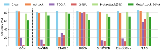
(a) Node classification accuracy on clean and attacked graphs on Cora

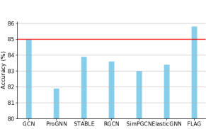
(b) Clean: performance comparison

Figure 1: Limitation of existing methods: Defenses suffer performance degradation under various attacks and on clean graph. 5% and 20% denote perturbation rates of MetaAttack.

In this paper, to tackle the above issues, we innovatively propose an invariant causal defense paradigm to achieve adversarial robustness across attacks. We aim to learn causal features that determine labels, ensuring that these features exhibit: (1) strong predictability for labels: the model should perform well on the clean graph; (2) invariant predictability across attacks: the model maintains good performance across attacks. We suggest that these two goals are exactly what an effective defense model should possess.

To learn causal features, we need to model and analyze the relationship between causal features with other variables. However, existing methods like structural causal models (SCMs) face challenges in grasping non-IID characteristics present in graph data, specifically the interactions (e.g., edges) between samples (e.g., nodes) [62]. To overcome the challenge, we design an interaction causal model [62] for graph adversarial attacks, which can capture the causalities between different samples. Next, we propose an Invariant causal DEfense method against adversarial Attacks, namely IDEA, to learn causal features. By analyzing the difference in attack impacts and the causal features’ characteristics, we design node-based and structure-based invariance objectives from an information-theoretic perspective. Under the linear assumption of causal relationships, we theoretically demonstrate that our IDEA yields causally invariant defense, thereby achieving graph adversarial robustness. Extensive experiments demonstrate that our IDEA attains state-of-the-art defense performance against all five attacks on each of the five datasets, emphasizing that IDEA possesses both strong and invariant predictability across attacks.

The primary contributions of this paper can be mainly summarized as:

1. New paradigm: We introduce an innovative invariant causal defense paradigm to achieve adversarial robusntess, offering a novel perspective on graph adversarial learning field.

2. Methodology: We propose IDEA method to learn causal features to achieve graph adversarial robustness. Through modeling and analyzing the causalities in graph adversarial attacks, we design two invariance objectives to learn causal features.

3. Experimental evaluation: Comprehensive experiments on five benchmarks demonstrate that IDEA significantly surpasses all baselines under both evasion and poisoning attacks, highlighting the strong and invariant predictability of IDEA.

2 Preliminary

In this section, we introduce the widely-used node classification task and graph neural networks. We also introduce the goal of graph adversarial robustness.

GNN for Node Classification. Given an attributed graph $G=(\mathcal{V},\mathcal{E},X)$, we denote $\mathcal{V}=\{1,2,...,n\}$ as the set of $n$ nodes, $\mathcal{E}\subseteq\mathcal{V}\times\mathcal{V}$ as the set of edges, and $X\in\mathbb{R}^{n\times d}$ as the attribute matrix with $d$-dimensional attributes. The class set $\mathcal{K}$ contains $K=|\mathcal{K}|$ classes. The goal [25, 24] is to assign labels for nodes based on the node attributes and network structure by learning a GNN classifier $f_{\theta}$. The objective is: $\min_{\theta}\sum_{i\in\mathcal{V}}[L(f_{\theta}(G)_{i},Y_{i})]$, where $Y_{i}$ denotes the ground-truth label of node $i$.

Graph adversarial robustness. The graph adversarial attack aims to find a perturbed graph $\hat{G}$ that maximizes the loss of GNN model [24]:

$$\max_{\hat{G}\in\mathcal{B}(G)}\sum_{i\in\mathcal{V}}[L(f_{\theta^{*}}(\hat{G})_{i},Y_{i})]\quad\quad s.t.,\quad\theta^{*}=\arg\min_{\theta}\sum_{i\in\mathcal{V}}[L(f_{\theta}(G_{\text{train}})_{i},Y_{i})].$$ (1)

Here, $\hat{G}$ is the perturbed graph chosen from the constraint set $\mathcal{B}(G)$, where the perturbing nodes, edges, and node attributes should not exceed the corresponding budget [24]. $G_{\text{train}}=G$ in evasion attacks, and $G_{\text{train}}=\hat{G}$ in poisoning attacks.

Defense methods aim to improve graph adversarial robustness, defending against any adversarial attack. The goal can be formulated as:

$$\min_{\theta}\max_{\hat{G}\in\mathcal{B}(G)}\sum_{i\in\mathcal{V}}[L(f_{\theta}(\hat{G})_{i},Y_{i})].$$ (2)

Existing defense methods suffer performance degradation under various attacks or on clean graphs. Adversarial training methods can only be optimized for the training adversarial examples, limiting their ability to generalize to unseen adversarial examples. While graph purification or robust aggregation methods, designed based on specific heuristic priors (such as local smoothness [56, 53, 25, 63, 33, 23] and low rank [25, 17]), are only effective for adversarial attacks that satisfy these priors and may even damage performance on clean graphs. Hence, there is an urgent need to design a defense method that performs well both on clean graphs and across various attacks.

3 Methodology

In this section, we propose an invariant causal defense paradigm by learning causal features that determine labels. We first model the causal relationships between causal features and other variables in graph adversarial attacks. Then, we propose an Invariant causal DEfense method against Attacks (IDEA) to learn causal features by designing goals based on the analysis of causalities, to achieve adversarial robustness.

3.1 Interaction Causal Model

To model non-IID characteristics in graph data, specifically the interactions (e.g. edges) between samples (e.g. nodes), we design an interaction causal model with explicit variables  for graph adversarial attacks, which captures the causality between different samples [62].

As shown in Figure 2 (left), we take an example of two connected nodes $i$ and $k$, and inspect the causal relationships among variables: input data $G_{i}$ (node $i$’s ego-network), label $Y_{i}$, causal feature $C_{i}$, perturbation $T_{i}$, attack domain $D_{i}$, and those variables of neighbor node $k$. We introduce the latent causal feature $C_{i}$ as an abstraction that causes both input $G_{i}$ and label $Y_{i}$. For example, in credit scoring, $C_{i}$ represents the asset, which determines both the individual’s subgraph $G_{i}$ (including attributes and connections) and their credit score $Y_{i}$. Besides, the causal feature $C_{i}$ influences neighbor’s $G_{k}$ due to network structure, which aligns with GNN studies [27, 53]. To model graph adversarial attack, we introduce perturbation $T_{i}$, and attack domain $D_{i}$ which is a latent factor that determines $T_{i}$, as shown in Figure 2 (left). Attack domain $D_{i}$ refers to a category of adversarial attacks based on their characteristics, such as attack type or attack strength. Here, $D_{i}$ and $T_{i}$ are considered as non-causal feature $N_{i}$ in graph adversarial attacks, which we aim to eliminate. Note that perturbation $T_{i}$ also impacts the ego-network $G_{k}$ of the neighbor $k$, due to edges between nodes.

We analyze these causal relationships and find that: (i) causal feature $C$ determines label $Y$, indicating that causal feature exhibits strong predictability for label; (ii) the causality between $C$ and $Y$ remains unchanged across attack domains, indicating the causal feature maintains invariant predictability across attack domains. These two properties of causal features align with the capabilities we expect the robust model to possess. Specifically, strong predictability enables model to perform well on clean graph, invariant predictability allows it to maintain good performance under various attacks. Next, we devote to designing a defense method to learn causal feature $C$.

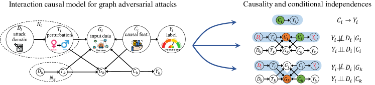
Figure 2: Left: Interaction causal model. Right: Causality and conditional independences.

3.2 IDEA: Invariant causal DEfense method against adversarial Attack

We propose Invariant causal DEfense against adversarial Attack (IDEA) to learn causal features. Our approach involves designing invariance objectives based on the distinctive properties of causal features and approximating losses accordingly. To reveal the diverse influence of attack domains, we introduce a domain partitioner for partitioning. We present the overall framework of IDEA.

3.2.1 Invariance Objective

To learn causal features, we design invariance objectives by analyzing the causality and conditional independences with the $d$-separation [42, 41] in Figure 2 (right). The observations are as follows:

1. $C_{i}\rightarrow Y_{i}$ denotes that causal feature $C$ causes label $Y$, i.e., $C$ has strong predictability for $Y$.

2. $Y_{i}\not\!\perp\!\!\!\perp D_{i}\mid G_{i}$ denotes that $Y$ and attack domain $D$ are associated, conditioned on $G$ (second path in Figure 2(right)), due to $G$ acting as a collider between $Y$ and $D$.

3. $Y_{i}\perp\!\!\!\perp D_{i}\mid C_{i}$ means that the causality of $Y$ determined by $C$ remains unchanged across attack domain $D$, i.e., $C$ has invariant predictability for $Y$ across various attack domains.

4. $Y_{i}\not\!\perp\!\!\!\perp D_{i}\mid G_{k}$ means that $Y_{i}$ and $D_{i}$ are associated, conditioned on $G_{k}$ of neighbor node $k$ (third path in Figure 2(right)), due to $G_{k}$ acting as a collider of $Y_{i}$ and $D_{i}$, similar to (2).

5. $Y_{i}\perp\!\!\!\perp D_{i}\mid C_{k}$ represents that given neighbor’s causal feature $C_{k}$, the relationship between $Y_{i}$ and attack domain $D_{i}$ remains unchanged.

Based on these observations, we analyze the characteristics of $C$ and propose three goals from the perspective of mutual information $I$ to guide model learning causal feature $C$. Let $\Phi$ represent the feature encoder, and $Z=\Phi(G)$ denote learned representation, which is intended to capture $C$.

• Predictive goal: $\max I\left(Z,Y\right)$ to guide $Z$ to have strong predictability for $Y$, based on (1).

• Node-based Invariance goal: $\min I\left(Y,D\mid Z\right)$. By comparing the conditional independences regarding $G_{i}$ in (2) and $C_{i}$ in (3), we propose this goal to guide $Z$ learning $C$ to obtain invariant predictability across different attack domains.

• Structural-based Invariance goal: $\min I\left(Y,D\mid Z_{\mathcal{N}}\right)$ to guide $Z_{\mathcal{N}}$ learning the causal feature for neighbor ($C_{\mathcal{N}}$), by comparing $G_{k}$ in (4) and $C_{k}$ in (5).

To sum up, the objective can be formulated as:

$$\max_{\Phi} I\left(\Phi(\hat{G}^{*}),Y\right)-\left[I\left(Y,D\mid\Phi(\hat{G}^{*})\right)+I\left(Y,D\mid\Phi(\hat{G}^{*})_{\mathcal{N}}\right)\right]$$ (3)

s.t. $$\hat{G}^{*}=\arg\min_{\hat{G}}I\left(\Phi(\hat{G}),Y\right),$$

Here, attack domain $D$ determines perturbation $T$, and $T$ influences the attacked graph $\hat{G}$. The objective guides IDEA to learn causal feature with strong predictability and invariant predictability across attack domains. Notably, the capability of this objective relies on the diversity of attack domain $D$, as detailed in Section 3.2.3. Proposition 2 demonstrates the effectiveness of our objective under the assumption of linear causalities. However, two challenges persist in solving Eq. (3): i) The objective is not directly optimizable due to the difficulty in estimating the mutual information of high-dimensional variables. ii) There may be a lack of diverse attack domains $D$, which are required to expose influence of the attack to promote better learning of invariant causal features.

3.2.2 Loss Approximation

We develop tractable losses for the above goals. For the predictive goal, we adopt variational approximation to solve it, similar to VIB [1, 31]. Specifically, by letting $q(y|z)$ be a variational approximation of distribution $p(y|z)$, we can derive the lower bound of the predictive goal:

$$I(Z,Y)=\mathbb{E}_{p(y,z)}\log\frac{p(y|z)}{p(y)}\geq\mathbb{E}_{p(x)}\mathbb{E}_{p(y|x)}\mathbb{E}_{p(z|x)}\log q\left(y\mid z\right),$$ (4)

where $x$ denotes the input data, i.e., the ego-network of node. To solve the lower bound, we employ encoder $h$ as a realization of $\Phi$ to learn representation. We assume $p(z\mid x)=\mathcal{N}\left(z\mid h^{\mu}(x),h^{\Sigma}(x)\right)$, where $h^{\mu}$ and $h^{\Sigma}$ output the mean $\mu$ and covariance matrix $\Sigma$ of $z$, respectively. We then leverage a re-parameterization technique [26] to overcome non-differentiability: $z=\mu+\epsilon*\Sigma$, where $\epsilon$ is a standard Gaussian random variable [31, 1]. Generally, encoder $h$ contains GNN and re-parameterization, and $h$ outputs $z=h(x,\epsilon)$. After that, we use a neural network $g$ as classifier to learn variation distribution $q(y|z)$ in Eq. (4), and obtain predictive loss $\mathcal{L}_{P}$:

$$\small\min_{g,h}\mathcal{L}_{P}\left(g,h,\hat{G}^{*}\right)=\min_{g,h}\sum_{i\in\mathcal{V}_{l}}L(g(h(\hat{G}^{*})_{i}),Y_{i}).$$ (5)

For the node-based invariance goal, the conditional mutual information is defined as:

$$I(Y,D|Z)= \ \mathbb{E}_{p(z)}\left[\mathbb{E}_{p(y,d\mid z)}\left[\log\frac{p(y,d\mid z)}{p(d\mid z)p(y\mid z)}\right]\right]$$ (6)

$$= \ \mathbb{E}_{p(z)}\left[\mathbb{E}_{p(y,d\mid z)}[\log p(y\mid z,d)-\log p(y\mid z)]\right].$$

We employ two variational distributions $q_{d}(y\mid z,d),\ q(y\mid z)$ with parameters to approximate $p(y\mid z,d),\ p(y\mid z)$. This allows us to obtain an estimation of $I(Y,D|Z)$:

$$\small\hat{I}(Y,D|Z)=\mathbb{E}_{p(z)}\left[\mathbb{E}_{p(y,d\mid z)}[\log q_{d}(y\mid z,d)-\log q(y\mid z)]\right].$$ (7)

To ensure that the above estimation serves as an upper bound of $I(Y,D|Z)$, we can minimize the KL-divergence $\mathbb{E}_{p(z,d)}KL[p(y\mid z,d)\|q_{d}(y\mid z,d)]$, similar to CLUB [13]. We prove that our goal $I(Y,D|Z)$ is minimized when both estimation $\hat{I}(Y,D|Z)$ and KL-divergence $\mathbb{E}_{p(z,d)}KL[p(y\mid z,d)\|q_{d}(y\mid z,d)]$ are minimized.

Proposition 1.

The node-based invariance goal $I(Y,D|Z)$ attains its lowest value if the following two quantities are minimized: $\mathbb{E}_{p(z,d)}KL[p(y\mid z,d)\|q_{d}(y\mid z,d)]$ and $\hat{I}(Y,D|Z)$.

The proof is in Appendix A.1. Then we use a neural network $g_{d}$ as classifier to learn $q_{d}(y\mid z,d)$. We optimize $\mathbb{E}_{p(z,d)}KL[p(y\mid z,d)\|q_{d}(y\mid z,d)]$ by minimizing $\sum_{i\in\mathcal{V}}L\left(g_{d}(h(\hat{G}^{*})_{i},D_{i}),Y_{i}\right)$, and optimize $\hat{I}(Y,D|Z)$ by minimizing $\sum_{i\in\mathcal{V}}\left[L\left(g(h(\hat{G}^{*})_{i}),Y_{i})-L(g_{d}(h(\hat{G}^{*})_{i},D_{i}),Y_{i}\right)\right]$. The node-based invariance loss $\mathcal{L}_{I}$:

$$\min_{g,g_{d},h} \mathcal{L}_{I}\left(g,g_{d},h,\hat{G}^{*},D\right)$$ (8)

$$=\min_{g,g_{d},h} \sum_{i\in\mathcal{V}}L\Bigr{(}g_{d}\bigl{(}h(\hat{G}^{*})_{i},D_{i}\bigr{)},Y_{i}\Bigr{)}+\alpha\left[L\Bigr{(}g\bigl{(}h(\hat{G}^{*})_{i}\bigr{)},Y_{i}\Bigr{)}-L\Bigr{(}g_{d}\bigl{(}h(\hat{G}^{*})_{i},D_{i}\bigr{)},Y_{i}\Bigr{)}\right],$$

where coefficient $\alpha$ is a hyper-parameter to balance the two terms.

The structural-based invariance goal aims to learn the causal feature for the neighbor. Similar to the above, this goal can be achieved by optimizing the structure-based invariance loss $\mathcal{L}_{E}$:

$$\min_{g,g_{d},h} \mathcal{L}_{E}\left(g,g_{d},h,\hat{G}^{*}D\right)$$ (9)

$$=\min_{g,g_{d},h} \sum_{i\in\mathcal{V},k\sim\mathcal{N}_{i}}L\Bigr{(}g_{d}\bigl{(}h(\hat{G}^{*})_{k},D_{i}\bigr{)},Y_{i}\Bigr{)}+\alpha\left[L\Bigr{(}g\bigl{(}h(\hat{G}^{*})_{k}\bigr{)},Y_{i}\Bigr{)}-L\Bigr{(}g_{d}\bigl{(}h(\hat{G}^{*})_{k},D_{i}\bigr{)},Y_{i}\Bigr{)}\right],$$

where $k$ is the sampled node from the neighbors $\mathcal{N}_{i}$ of node $i$.

In summary, the loss function consists of the predictive loss and the newly proposed two invariance loss terms, formally written as follows:

$$\!\min_{g,g_{d},h} \mathcal{L}_{P}\left(g,h,\hat{G}^{*}\right)+\mathcal{L}_{I}\left(g,g_{d},h,\hat{G}^{*},D\right)+\mathcal{L}_{E}\left(g,g_{d},h,\hat{G}^{*},D\right)$$ (10)

s.t. $$\hat{G}^{*}=\arg\max_{\hat{G}}\mathcal{L}_{P}\left(g,h,\hat{G}\right).$$

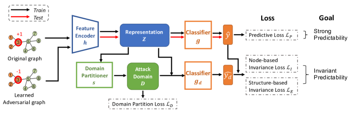
Figure 3: Overall architecture of our IDEA method. The black arrows denote the workflow of IDEA during training, while the red arrows denote how IDEA predicts in the test phase.

3.2.3 Domain Construction

For attack domain $D$ in Eq. (10), straightforward partitioning ways include dividing by attack type or strength. However, these approaches may yield an extremely limited number and diversity of domains. Intuitively, attack domains should be both sufficiently numerous [44, 2] and distinct from each other [14, 2] to reveal the various effects of attacks. To this end, we leverage a neural network $s$ as domain partitioner to find an appropriate partitioning. The partitioner $s$ allows for adjustable attack domain numbers. We ensure the diversity of domains by minimizing the co-linearity between the samples from different domains. We adopt Pearson correlation coefficient (PCCs) to measure of linear correlation between two sets of data. The loss function $\mathcal{L}_{D}$:

$$\min_{s}\mathcal{L}_{D}\left(s,h\right)= \min_{s}\sum_{D\neq D^{\prime}}\textbf{PCCs}\left(r^{D},r^{D^{\prime}}\right)$$ (11)

$$r^{D}= \mathbb{E}_{i\in\mathcal{V}^{D}}\left[h(\hat{G}^{*})_{i}\left(g(h(\hat{G}^{*})_{i})-Y_{i}\right)\right],\mathcal{V}^{D}=\left\{i|(s(h(\hat{G}^{*}))_{i}=D\right\},$$

where $\mathcal{V}^{D}$ denotes nodes assigned to domain $D$ by partitioner $s$, $r^{D}$ denotes the representation of $\mathcal{V}^{D}$. The form of $r^{D}$ aids in proving IDEA achieving adversarial robustness (proof of Proposition 2).

3.2.4 Overall Framework

According to the above analysis, the overall loss function of IDEA is formulated as:

$$\!\min_{g,g_{d},h} \mathcal{L}_{P}\left(g,h,\hat{G}^{*}\right)+\mathcal{L}_{I}\left(g,g_{d},h,s^{*},\hat{G}^{*}\right)+\mathcal{L}_{E}\left(g,g_{d},h,s^{*},\hat{G}^{*}\right)]$$ (12)

s.t. $$\hat{G}^{*}=\arg\max_{\hat{G}}\mathcal{L}_{P}\left(g,h,\hat{G}\right),\quad s^{*}=\arg\min_{s}\mathcal{L}_{D}\left(s,h\right).$$

The overall architecture of IDEA is illustrated in Figure 3. The IDEA model consists of four parts: an encoder $h$ to learn the node representation, i.e., causal feature; a classifier $g$ for final classification; a domain-based classifier $g_{d}$ for invariance goals; and a domain partitioner $s$ to provide the partition of attack domain. We also provide the algorithm in Appendix B.

Through theoretical analysis in Proposition 2, IDEA produces causally invariant defenders under the linear assumption of causal relationship [2], enabling graph adversarial robustness.

Proposition 2.

Assume that $Y=C\cdot\gamma+\epsilon,\ \hat{G}=\psi\left(C,N\right),$ where $\gamma$ and $\psi$ denote the intrinsic mechanism how $C$ determines $Y$ and $\hat{G}$, respectively, and noise term $\epsilon$ satisfies $\mathbb{E}\left[\epsilon\right]=0$. Suppose there exists a function $\tilde{\psi}$ satisfying $\tilde{\psi}(\hat{G})=C$, which can extract causal feature $C$, $\tilde{\psi}^{\top}\gamma$ is the ground truth predictor (ideal defender). Let encoder $\Phi\in\mathbb{R}^{m\times m}$ have rank $r$, and let $\omega$ be a classifier, then $\Phi^{\top}\omega$ is a defender. If $\Phi^{\top}\omega$ fulfills the following conditions in training attack domain set $\mathcal{D}_{\text{tr}}$:
(1) Eq. (3), $I\left(\Phi(\hat{G}),Y\right)-\left[I\left(Y,D\mid\Phi(\hat{G})\right)+I\left(Y,D\mid\Phi(\hat{G})_{\mathcal{N}}\right)\right]$ is maximized,
(2) $\left\{\mathbb{E}_{\hat{G}^{D}}\left[\hat{G}^{D}\hat{G}^{D^{\top}}\right]\left(\Phi^{\top}w-\tilde{\psi}^{\top}\gamma\right)\right\}_{D\in\mathcal{D}_{\text{tr}}}$ is linearly independent, which means samples across distinct domains are dissimilar, and $\operatorname{dim}\left(\operatorname{span}\left(\left\{\mathbb{E}_{\hat{G}_{i}}\left[\hat{G}_{i}\hat{G}_{i}^{\top}\right]\left(\Phi^{\top}w-\tilde{\psi}^{\top}\gamma\right)\right\}_{i\in\mathcal{V}}\right)\right)>m-r$,
then $\Phi^{\top}\omega=\tilde{\psi}^{\top}\gamma$ is causal invariant defender for all attack domain set $\mathcal{D}_{\text{all}}$.

The proof of Proposition 2 is available in Appendix A.2. Note that condition (1) is aligns with minimizing the losses $\mathcal{L}_{P}$, $\mathcal{L}_{I}$, and $\mathcal{L}_{E}$ in Eq.(12). In condition (2), the first term corresponds to minimizing $\mathcal{L}_{D}$ in Eq.(12), while the second term implies the diversity of adversarial examples, common in graph. Proposition 2 serves as a theoretical validation for the effectiveness of IDEA.

Table 1: Accuracy(%) of targets under evasion attacks. The best and second-best are highlighted. Parentheses denote IDEA’s relative increase compared to second-best. ’-’ for out-of-memory (OOM).

Dataset	Attack	GCN	GAT	ProGNN	STABLE	RGCN	SimpGCN	ElasticGNN	FLAG	IDEA
Cora	Clean	85.0 $\pm$ 0.5	84.6 $\pm$ 0.8	81.9 $\pm$ 1.2	83.9 $\pm$ 0.6	83.6 $\pm$ 0.7	83.0 $\pm$ 1.2	83.4 $\pm$ 1.9	85.8 $\pm$ 0.6	88.4 $\pm$ 0.6  ( $\uparrow$ 3.0%)
	nettack	83.0 $\pm$ 0.5	81.7 $\pm$ 0.7	79.9 $\pm$ 1.1	21.5 $\pm$ 4.8	81.7 $\pm$ 0.6	82.0 $\pm$ 1.2	79.4 $\pm$ 1.7	84.8 $\pm$ 0.6	85.4 $\pm$ 0.7  ( $\uparrow$ 0.8%)
	PGD	44.2 $\pm$ 3.4	26.7 $\pm$ 7.6	19.6 $\pm$ 2.2	32.2 $\pm$ 0.2	80.5 $\pm$ 0.4	9.0 $\pm$ 2.2	29.0 $\pm$ 5.5	60.2 $\pm$ 2.4	83.6 $\pm$ 2.1  ( $\uparrow$ 3.8%)
	TDGIA	20.2 $\pm$ 2.3	33.7 $\pm$ 14.9	15.4 $\pm$ 1.7	30.9 $\pm$ 2.4	79.9 $\pm$ 0.9	13.5 $\pm$ 1.2	18.0 $\pm$ 1.2	57.2 $\pm$ 3.0	81.2 $\pm$ 2.5  ( $\uparrow$ 1.6%)
	G-NIA	2.3 $\pm$ 0.5	5.2 $\pm$ 3.1	4.2 $\pm$ 0.8	25.8 $\pm$ 10.1	81.3 $\pm$ 0.9	11.5 $\pm$ 8.1	11.2 $\pm$ 3.7	64.8 $\pm$ 2.0	85.3 $\pm$ 1.2  ( $\uparrow$ 4.9%)
	AVG	47.0 $\pm$ 37.0	46.4 $\pm$ 35.2	40.2 $\pm$ 37.6	38.9 $\pm$ 25.5	81.4 $\pm$ 1.4	39.8 $\pm$ 39.0	44.2 $\pm$ 34.6	70.6 $\pm$ 13.7	84.8 $\pm$ 2.7  ( $\uparrow$ 4.1%)
Citeseer	Clean	73.6 $\pm$ 0.6	74.7 $\pm$ 1.0	74.1 $\pm$ 0.9	75.2 $\pm$ 0.5	74.6 $\pm$ 0.5	74.9 $\pm$ 1.3	74.0 $\pm$ 1.3	74.7 $\pm$ 0.9	82.0 $\pm$ 1.9  ( $\uparrow$ 9.1%)
	nettack	72.6 $\pm$ 0.7	72.6 $\pm$ 1.8	71.5 $\pm$ 0.9	20.8 $\pm$ 8.5	73.2 $\pm$ 0.6	74.5 $\pm$ 1.1	71.8 $\pm$ 1.5	73.6 $\pm$ 1.2	78.8 $\pm$ 1.6  ( $\uparrow$ 5.7%)
	PGD	52.7 $\pm$ 4.5	54.5 $\pm$ 5.3	41.4 $\pm$ 4.1	17.7 $\pm$ 6.2	70.1 $\pm$ 1.1	48.2 $\pm$ 13.9	39.1 $\pm$ 6.0	60.1 $\pm$ 2.5	76.9 $\pm$ 3.4  ( $\uparrow$ 9.8%)
	TDGIA	23.0 $\pm$ 3.8	44.7 $\pm$ 11.2	16.9 $\pm$ 2.1	15.5 $\pm$ 5.3	63.8 $\pm$ 7.4	28.1 $\pm$ 11.1	18.2 $\pm$ 3.6	57.5 $\pm$ 1.7	75.9 $\pm$ 3.9  ( $\uparrow$ 19.0%)
	G-NIA	15.0 $\pm$ 3.6	13.6 $\pm$ 3.6	22.5 $\pm$ 4.8	18.5 $\pm$ 6.6	32.1 $\pm$ 6.4	54.4 $\pm$ 16.8	30.2 $\pm$ 4.2	68.0 $\pm$ 0.9	79.4 $\pm$ 3.0  ( $\uparrow$ 16.8%)
	AVG	47.4 $\pm$ 27.3	52.0 $\pm$ 24.9	45.3 $\pm$ 26.7	29.5 $\pm$ 25.6	62.8 $\pm$ 17.7	56.0 $\pm$ 19.6	46.6 $\pm$ 25.1	66.8 $\pm$ 7.8	78.6 $\pm$ 2.4  ( $\uparrow$ 17.7%)
Reddit	Clean	84.9 $\pm$ 0.6	88.5 $\pm$ 0.3	66.2 $\pm$ 3.1	83.6 $\pm$ 0.4	68.0 $\pm$ 1.7	50.2 $\pm$ 8.3	72.7 $\pm$ 0.6	86.9 $\pm$ 0.4	90.8 $\pm$ 0.3  ( $\uparrow$ 2.7%)
	nettack	84.8 $\pm$ 0.5	87.9 $\pm$ 0.4	68.8 $\pm$ 3.1	3.6 $\pm$ 3.2	67.0 $\pm$ 1.7	49.5 $\pm$ 8.4	71.4 $\pm$ 0.7	85.5 $\pm$ 0.4	89.1 $\pm$ 0.5  ( $\uparrow$ 1.4%)
	PGD	46.0 $\pm$ 1.6	30.8 $\pm$ 2.5	20.0 $\pm$ 5.4	3.6 $\pm$ 1.5	53.1 $\pm$ 2.1	9.8 $\pm$ 3.3	19.0 $\pm$ 1.0	72.1 $\pm$ 0.9	81.6 $\pm$ 0.9  ( $\uparrow$ 13.2%)
	TDGIA	24.1 $\pm$ 1.6	32.8 $\pm$ 3.8	9.0 $\pm$ 3.0	3.6 $\pm$ 1.4	44.3 $\pm$ 1.9	5.5 $\pm$ 1.6	8.3 $\pm$ 0.6	73.1 $\pm$ 0.7	81.3 $\pm$ 0.6  ( $\uparrow$ 11.1%)
	G-NIA	1.0 $\pm$ 0.8	2.5 $\pm$ 1.1	4.0 $\pm$ 3.6	4.7 $\pm$ 2.2	5.0 $\pm$ 2.0	5.3 $\pm$ 3.7	3.3 $\pm$ 0.7	76.9 $\pm$ 1.2	84.2 $\pm$ 1.1  ( $\uparrow$ 9.5%)
	AVG	48.2 $\pm$ 37.1	48.5 $\pm$ 38.2	33.6 $\pm$ 31.5	19.8 $\pm$ 35.6	47.5 $\pm$ 25.7	24.1 $\pm$ 23.6	34.9 $\pm$ 34.4	78.9 $\pm$ 6.9	85.4 $\pm$ 4.4  ( $\uparrow$ 8.2%)
ogbn- products	Clean	63.9 $\pm$ 0.7	69.6 $\pm$ 0.4	49.7 $\pm$ 2.4	67.6 $\pm$ 0.8	64.3 $\pm$ 0.4	57.7 $\pm$ 2.2	57.9 $\pm$ 0.9	67.6 $\pm$ 0.7	76.1 $\pm$ 0.4  ( $\uparrow$ 9.2%)
	nettack	63.3 $\pm$ 0.6	62.1 $\pm$ 2.1	50.1 $\pm$ 3.1	14.9 $\pm$ 1.4	62.1 $\pm$ 0.8	56.1 $\pm$ 2.4	52.6 $\pm$ 0.9	65.8 $\pm$ 0.5	74.4 $\pm$ 0.6  ( $\uparrow$ 13.1%)
	PGD	32.2 $\pm$ 0.9	25.0 $\pm$ 0.8	17.5 $\pm$ 1.0	14.3 $\pm$ 1.8	34.8 $\pm$ 0.9	17.8 $\pm$ 1.5	21.2 $\pm$ 0.5	54.0 $\pm$ 0.6	67.9 $\pm$ 0.6  ( $\uparrow$ 25.7%)
	TDGIA	23.1 $\pm$ 1.0	16.9 $\pm$ 1.1	11.0 $\pm$ 0.5	16.5 $\pm$ 1.9	28.0 $\pm$ 0.9	16.5 $\pm$ 2.2	16.9 $\pm$ 0.8	49.5 $\pm$ 1.0	64.9 $\pm$ 0.9  ( $\uparrow$ 31.2%)
	G-NIA	2.7 $\pm$ 1.0	3.6 $\pm$ 2.0	2.2 $\pm$ 0.8	9.9 $\pm$ 5.2	7.1 $\pm$ 2.6	8.6 $\pm$ 4.5	3.3 $\pm$ 0.6	54.2 $\pm$ 0.8	65.6 $\pm$ 1.1  ( $\uparrow$ 21.0%)
	AVG	37.1 $\pm$ 26.5	35.5 $\pm$ 28.9	26.1 $\pm$ 22.4	24.7 $\pm$ 24.1	39.3 $\pm$ 24.1	31.3 $\pm$ 23.6	30.4 $\pm$ 23.7	58.2 $\pm$ 8.0	69.8 $\pm$ 5.2  ( $\uparrow$ 19.8%)
ogbn- arxiv	Clean	65.3 $\pm$ 0.3	65.2 $\pm$ 0.1	-	-	60.2 $\pm$ 1.0	-	58.0 $\pm$ 0.1	61.0 $\pm$ 0.7	66.7 $\pm$ 0.4  ( $\uparrow$ 2.1%)
	PGD	41.1 $\pm$ 1.0	22.6 $\pm$ 1.9	-	-	37.8 $\pm$ 2.0	-	29.9 $\pm$ 0.6	24.2 $\pm$ 2.8	52.9 $\pm$ 1.0  ( $\uparrow$ 28.8%)
	TDGIA	33.1 $\pm$ 1.6	9.7 $\pm$ 1.8	-	-	27.5 $\pm$ 2.1	-	20.5 $\pm$ 0.9	29.3 $\pm$ 2.3	53.2 $\pm$ 0.8  ( $\uparrow$ 60.8%)
	G-NIA	4.6 $\pm$ 0.4	2.5 $\pm$ 0.3	-	-	5.6 $\pm$ 0.8	-	14.6 $\pm$ 0.1	11.5 $\pm$ 1.1	40.5 $\pm$ 1.6  ( $\uparrow$ 251.9%)
	AVG	36.0 $\pm$ 25.0	25.0 $\pm$ 28.1	-	-	32.8 $\pm$ 22.7	-	30.7 $\pm$ 19.2	31.5 $\pm$ 21.0	53.3 $\pm$ 10.7  ( $\uparrow$ 48.0%)

4 Experiments

Datasets. To evaluate the adaptability of IDEA across various datasets, we conduct node classification experiments on 5 diverse network benchmarks: three citation networks (Cora [5], Citeseer [5], and obgn-arxiv [22]), a social network (Reddit [21, 61]), and a product co-purchasing network (ogbn-products [22]). The statistics and details of datasets are provided in Appendix D.1.

Attack methods and defense baselines. To demonstrate the effectiveness of our IDEA, we compare IDEA with the state-of-the-art defense methods, including: traditional GNNs (GCN [27], GAT [53]), graph purification (ProGNN [25], STABLE [33]), robust aggregation (RGCN [65], SimPGCN [23], ElasticGNN [37]), and adversarial training (FLAG [28]). The details are described in Appendix D.2. We evaluate the robustness of IDEA using five attacks, including a representative poisoning attack (MetaAttack [68]) and four evasion attacks (nettack [67], PGD [39], TDGIA [66], G-NIA [49]). The details of attacks are provided in Appendix D.3.

Implementation. For each dataset, we randomly split 10%/10%/80% of nodes for training, validation and test, following [25, 23, 37, 33]. For each experiment, we report the average performance and the standard deviation of 10 runs. We employ the widely-used DeepRobust [35] library for the attack and defense methods. We tune their hyper-parameters according validation set. Note that the evasion attacks are targeted attacks, and we randomly sample $20\%$ of all nodes from the test set as targets. Nettack perturbs 20% edges, while node injection attacks (PGD, TDGIA, and G-NIA) inject 20% nodes and edges. MetaAttack is untargeted, performance is reported on the test set with perturbation rates from 0% to 20%, following [37, 33]. For IDEA, our backbone model is GCN, which is used for the encoder $h$. We tune the hyper-parameters from the following range: the coefficient $\alpha$ over $\{10,25,100,150\}$, the number of domains over $\{2,5,10,20\}$. The details are in Appendix D.4.

4.1 Robustness against Evasion Attacks

We conduct experiments under four evasion attacks (nettack, PGD, TDGIA, and G-NIA), and show the accuracy of target nodes in Table 1. We also report the average accuracy of clean and attacked graphs, along with standard deviation of accuracy across these graphs, denoted as AVG. Note that we exclude nettack from ogbn-arxiv evaluation due to its lack of scalability. GCN and GAT exhibit high accuracy on clean graphs, however, their accuracy significantly declines under PGD, TDGIA, and G-NIA. Defense methods suffer from inconsistent performance across various attacks, with some, e.g., ProGNN (81.9%) and RGCN (83.6%), even experiencing a decline on Clean. For graph purification methods, ProGNN and STABLE perform poorly under most attacks, maybe because they require retraining to achieve defensive effects, rendering them unsuitable for evasion attacks. RGCN, SimPGCN, and ElasticGNN perform well against nettack; however, they suffer from performance degradation on clean graphs, which is undesirable. Adversarial training FLAG outperforms other baselines but exhibits unsatisfactory defense on Cora, Citeseer, and ogbn-arxiv.

Our proposed method, IDEA, achieves the best performance on Clean and across all attacks, significantly outperforming all baselines on all datasets. On Clean, IDEA exhibits the best performance primarily due to its ability to learn causal features that have strong label predictability. Furthermore, IDEA’s performance remains good consistency under both clean graphs and various attacks, evidenced by the low standard deviation in AVG. This emphasizes its invariant predictability across all attacks. For instance, on Citeseer, IDEA’s standard deviation across graphs is a only 2.4, while the runner-up, FLAG, reaches 7.8. These results demonstrate that IDEA possesses both strong predictability (high accuracy on Clean) and invariant predictability (sustained accuracy across attacks).

Table 2: Accuracy(%) of test set under poisoning attack (MetaAttack).

Dataset	Pt.	GCN	GAT	ProGNN	STABLE	RGCN	SimPGCN	ElasticGNN	FLAG	IDEA
Cora	0%	83.6 $\pm$ 0.5	83.5 $\pm$ 0.5	83.0 $\pm$ 0.2	85.6 $\pm$ 0.6	82.6 $\pm$ 0.3	81.9 $\pm$ 1.0	85.8 $\pm$ 0.4	83.4 $\pm$ 0.3	87.1 $\pm$ 0.7  ( $\uparrow$ 1.6%)
	5%	77.8 $\pm$ 0.6	80.3 $\pm$ 0.5	82.3 $\pm$ 0.5	81.4 $\pm$ 0.5	77.5 $\pm$ 0.5	77.6 $\pm$ 0.7	82.2 $\pm$ 0.9	80.9 $\pm$ 0.3	84.6 $\pm$ 1.0  ( $\uparrow$ 2.8%)
	10%	74.9 $\pm$ 0.7	78.5 $\pm$ 0.6	79.0 $\pm$ 0.6	80.5 $\pm$ 0.6	73.7 $\pm$ 1.2	75.7 $\pm$ 1.1	78.8 $\pm$ 1.7	78.8 $\pm$ 0.9	84.1 $\pm$ 0.6  ( $\uparrow$ 4.5%)
	15%	67.8 $\pm$ 1.2	73.6 $\pm$ 0.8	76.4 $\pm$ 1.3	78.6 $\pm$ 0.4	70.2 $\pm$ 0.6	72.7 $\pm$ 2.8	77.2 $\pm$ 1.6	75.0 $\pm$ 0.7	83.3 $\pm$ 0.6  ( $\uparrow$ 6.1%)
	20%	61.6 $\pm$ 1.1	66.6 $\pm$ 0.8	73.3 $\pm$ 1.6	77.8 $\pm$ 1.1	62.7 $\pm$ 0.7	70.3 $\pm$ 4.6	70.5 $\pm$ 1.3	70.2 $\pm$ 1.1	82.6 $\pm$ 0.7  ( $\uparrow$ 6.2%)
Citeseer	0%	73.3 $\pm$ 0.3	74.4 $\pm$ 0.8	73.3 $\pm$ 0.7	75.8 $\pm$ 0.4	74.4 $\pm$ 0.3	74.4 $\pm$ 0.7	73.8 $\pm$ 0.6	72.8 $\pm$ 0.8	80.3 $\pm$ 1.0  ( $\uparrow$ 5.8%)
	5%	70.2 $\pm$ 0.8	72.3 $\pm$ 0.5	72.9 $\pm$ 0.6	74.1 $\pm$ 0.6	71.7 $\pm$ 0.3	73.3 $\pm$ 1.0	72.9 $\pm$ 0.5	71.1 $\pm$ 0.6	78.7 $\pm$ 0.5  ( $\uparrow$ 6.2%)
	10%	68.0 $\pm$ 1.4	70.3 $\pm$ 0.7	72.5 $\pm$ 0.8	73.5 $\pm$ 0.4	69.3 $\pm$ 0.4	72.0 $\pm$ 1.0	72.6 $\pm$ 0.4	69.2 $\pm$ 0.6	77.6 $\pm$ 0.9  ( $\uparrow$ 5.7%)
	15%	65.2 $\pm$ 0.9	67.7 $\pm$ 1.0	72.0 $\pm$ 1.1	73.2 $\pm$ 0.5	66.0 $\pm$ 0.2	70.8 $\pm$ 1.3	71.9 $\pm$ 0.7	66.5 $\pm$ 0.8	75.5 $\pm$ 0.9  ( $\uparrow$ 3.3%)
	20%	60.1 $\pm$ 1.4	64.3 $\pm$ 1.0	70.0 $\pm$ 2.3	72.8 $\pm$ 0.5	61.2 $\pm$ 0.5	70.0 $\pm$ 1.7	64.7 $\pm$ 0.8	64.1 $\pm$ 0.8	74.9 $\pm$ 0.9  ( $\uparrow$ 2.9%)
Reddit	0%	84.5 $\pm$ 0.5	88.0 $\pm$ 0.3	73.4 $\pm$ 2.8	86.6 $\pm$ 0.2	78.2 $\pm$ 0.6	51.4 $\pm$ 7.6	83.8 $\pm$ 0.3	84.6 $\pm$ 0.2	91.2 $\pm$ 0.3  ( $\uparrow$ 3.6%)
	5%	81.0 $\pm$ 0.8	86.1 $\pm$ 0.6	73.9 $\pm$ 1.2	81.5 $\pm$ 0.4	73.9 $\pm$ 1.7	34.8 $\pm$ 9.9	80.6 $\pm$ 0.5	83.6 $\pm$ 0.4	89.7 $\pm$ 0.3  ( $\uparrow$ 4.2%)
	10%	72.1 $\pm$ 0.6	78.8 $\pm$ 0.8	63.2 $\pm$ 1.2	75.9 $\pm$ 0.5	57.8 $\pm$ 1.3	27.3 $\pm$ 7.8	70.4 $\pm$ 1.0	72.2 $\pm$ 0.8	88.8 $\pm$ 0.2  ( $\uparrow$ 12.7%)
	15%	70.1 $\pm$ 1.7	76.0 $\pm$ 1.6	59.9 $\pm$ 1.4	73.8 $\pm$ 0.4	53.3 $\pm$ 1.4	25.0 $\pm$ 6.4	68.7 $\pm$ 0.6	66.3 $\pm$ 1.2	88.3 $\pm$ 0.3  ( $\uparrow$ 16.2%)
	20%	67.9 $\pm$ 1.4	72.7 $\pm$ 1.9	56.7 $\pm$ 0.9	71.7 $\pm$ 0.5	51.5 $\pm$ 2.8	19.0 $\pm$ 4.5	67.4 $\pm$ 0.6	63.7 $\pm$ 0.5	87.9 $\pm$ 0.4  ( $\uparrow$ 20.8%)
ogbn- products	0%	63.0 $\pm$ 0.7	68.6 $\pm$ 0.4	64.3 $\pm$ 2.0	70.5 $\pm$ 0.5	63.0 $\pm$ 0.5	57.1 $\pm$ 2.1	72.7 $\pm$ 0.2	66.3 $\pm$ 0.4	75.2 $\pm$ 0.3  ( $\uparrow$ 3.5%)
	5%	49.6 $\pm$ 0.9	64.4 $\pm$ 0.3	50.0 $\pm$ 2.4	58.7 $\pm$ 0.7	40.0 $\pm$ 1.1	31.9 $\pm$ 10.3	61.0 $\pm$ 0.7	57.3 $\pm$ 0.7	73.6 $\pm$ 0.5  ( $\uparrow$ 14.2%)
	10%	39.4 $\pm$ 1.1	54.4 $\pm$ 0.7	43.4 $\pm$ 1.9	50.5 $\pm$ 0.5	33.4 $\pm$ 0.9	26.7 $\pm$ 8.1	52.3 $\pm$ 0.7	46.7 $\pm$ 0.7	72.9 $\pm$ 0.5  ( $\uparrow$ 34.0%)
	15%	34.4 $\pm$ 1.1	46.7 $\pm$ 0.7	38.4 $\pm$ 1.8	44.6 $\pm$ 0.8	29.9 $\pm$ 1.0	20.3 $\pm$ 6.6	48.6 $\pm$ 0.4	42.7 $\pm$ 0.5	72.0 $\pm$ 0.5  ( $\uparrow$ 48.1%)
	20%	31.2 $\pm$ 1.0	41.9 $\pm$ 1.2	34.0 $\pm$ 2.5	40.3 $\pm$ 0.7	27.8 $\pm$ 0.8	16.0 $\pm$ 2.1	46.3 $\pm$ 0.4	39.3 $\pm$ 0.6	71.2 $\pm$ 0.8  ( $\uparrow$ 53.8%)

4.2 Robustness against Poisoning Attacks

We evaluate IDEA’s robustness under poisoning attacks, employing the widely-adopted MetaAttack [68] and varying the perturbation rate (the rate of changing edges) from 0 to 20% following [37, 33]. We exclude ogbn-arxiv since MetaAttack cannot handle large graphs. Table 2 shows that all methods’ accuracy decreases as perturbation rate increases. Among baselines, graph purification methods demonstrate better defense performance, with STABLE outperforming others on Cora and Citeseer. RGCN and SimPGCN resist attacks only at low perturbation rates. The adversarial training FLAG brings less improvement than it does under evasion attacks. Maybe due to its training on evasion attacks, leading to poor generalization for poisoning attacks.

For ours, IDEA also achieves the state-of-the-art performance under all perturbation rates on all datasets, significantly outperforming all baselines. When the attack strength becomes larger, our IDEA still maintains good performance, demonstrating that IDEA has the invariant prediction ability across perturbations.

4.3 Ablation Study

We analyze the influence of each part of IDEA through experiments on invariance goals and domain construction. We implement four variants of IDEA, including IDEA removing the node-based invariance goal (IDEA w/o $\mathcal{L}_{I}$), IDEA removing the structure-based invariance goal $\mathcal{L}_{E}$ (IDEA w/o $\mathcal{L}_{E}$), IDEA removing both invariance goals (IDEA w/o $\mathcal{L}_{I}$ and $\mathcal{L}_{E}$), and IDEA removing domain partition (IDEA w/o $\mathcal{L}_{D}$). IDEA w/o $\mathcal{L}_{I}$ and $\mathcal{L}_{E}$ only optimizes the predictive loss, which can be regarded as an adversarial training version of IDEA, which can verify the benefit brought by learning causal features. We take the results on clean graph and evasion attacks on Cora as an illustration.

As shown in Figure 5, all variants exhibit a decline compared to IDEA (red), highlighting the significance of both invariance goals and domain construction. Specifically, IDEA w/o $\mathcal{L}_{I}$ and $\mathcal{L}_{E}$ (blue) suffers the largest drop, highlighting our objectives’ benefits since IDEA is much more robust than simple adversarial training using same adversarial examples. The performance decline of IDEA w/o $\mathcal{L}_{E}$ (orange) illustrates the significant advantages of the structural-based invariance goal, especially on clean graph, highlighting the benefits of modeling the interactions between samples. IDEA w/o $\mathcal{L}_{D}$ (green) displays a large standard deviation, with the error bar much larger than that of IDEA, emphasizing the stability achieved through the diverse attack domains.

More detailed hyper-parameter analysis regarding coefficient $\alpha$ and the number of attack domains can be found in Appendix D.5.

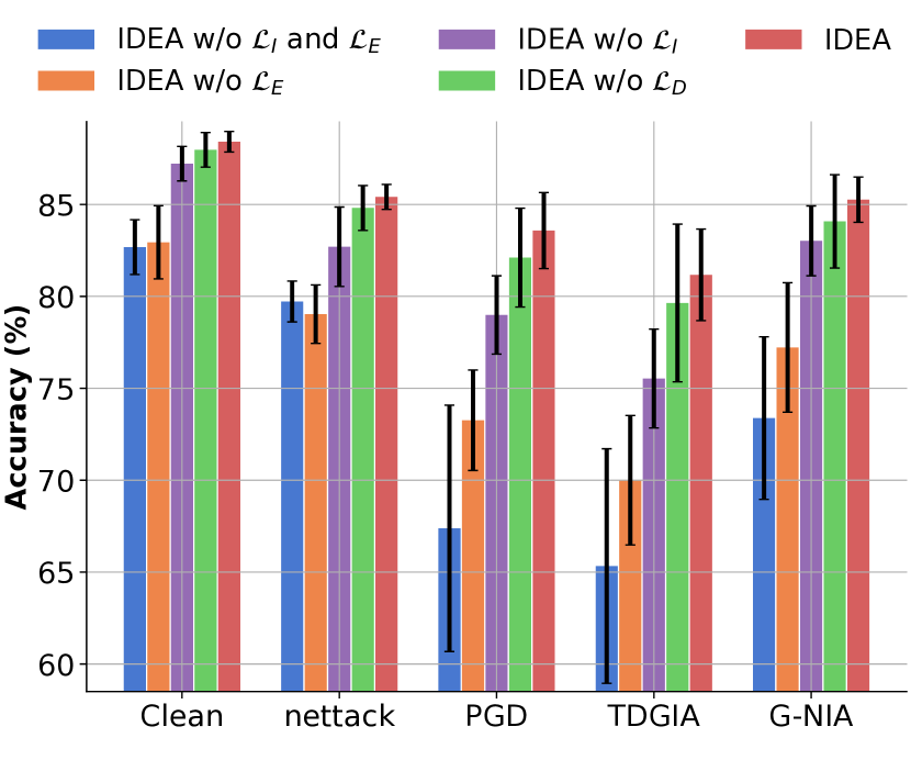
Figure 4: Ablation Study.

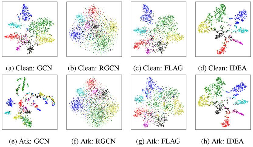
Figure 5: Visualizing learned features: clean and attacked graphs.

4.4 Visualization

We further visualize the learned features with t-SNE technique [52] to show whether IDEA learns the features that have strong and invariant predictability. Figure 5 illustrates the feature learned by GCN, RGCN, FLAG, and IDEA on clean graph and under the strongest G-NIA attack on Cora. As shown in Figure 5, existing methods either learn discriminative features on Clean but destroyed under attack (GCN and FLAG), or learn features are mixed (RGCN).

For our IDEA, in Figure 5(d,h), the features learned by IDEA can be distinguished by labels. Specifically, IDEA’s learned features are similar for nodes with the same label and distinct for different labels, emphasizing features’ strong predictability for labels. Furthermore, the features in Figure 5(d) on the clean graph and those in Figure 5(h) on the attacked graph exhibit nearly the same distributions. This observation demonstrates that the relationship between features and labels can remain invariant across attacks, thus exhibiting invariant predictability.

5 Conclusion

In this paper, we propose a novel causal defense paradigm by learning the causal features that have strong and invariant predictability across attacks, which brings a new perspective on graph adversarial learning. Then, we design two invariance objectives to learn causal features and propose IDEA method to achieve graph adversarial robustness. Extensive experiments demonstrate that our IDEA significantly outperforms all the baselines under both evasion attack and poisoning attacks on five benchmark datasets, emphasizing that IDEA possesses both strong and invariant predictability across attacks. We believe the causal defense paradigm is a promising research direction, and look forward to further exploration in the future.

Broader impact. Our paper focuses on a defense method, aiming to resist adversarial attacks and enhance the reliability of Graph Neural Networks (GNN) in practical applications. We do not foresee any significant negative impact associated with this research.

Limitation. Our work mainly focuses on graph data. It is challenging for us to identify causal features like those in image data, due to its inherent complexity and visualization limitations. Instead, we visualize the relationships between causal features and labels, aiming to show that these causal variables can have both strong predictability for labels and invariant predictability across attacks. In addition, although empirical evidence supports IDEA’s superiority across various datasets, theoretically, we can only establish invariant defender when assuming a linear causality. We believe studying theoretical guarantee for general scenarios is a valuable research question.

Appendix A Proofs

A.1 Proof for Proposition 1

Proof.

The difference between $\hat{I}(Y,D|Z)$ and $I(Y,D|Z)$ could be written as

$$\hat{I}(Y,D|Z)-I(Y,D|Z)$$ (13)

$$= \ \mathbb{E}_{p(z)}\biggl{[}\mathbb{E}_{p\left(y,d|z\right)}\Bigl{[}\left[\log q_{d}(y\mid z,d)-\log q(y|z)\right]-\left[\log p(y\mid z,d)-\log p(y\mid z)\right]\Bigr{]}\biggr{]}$$

$$= \ \mathbb{E}_{p(z)}\left[\mathbb{E}_{p(y,d\mid z)}\left[\log\frac{p(y\mid z)}{q(y\mid z)}-\log\frac{p(y\mid z,d)}{q_{d}(y\mid z,d)}\right]\right]$$

$$= \ \mathbb{E}_{p(z)}\left[\mathbb{E}_{p(y\mid z)}\left[\log\frac{p(y\mid z)}{q(y\mid z)}\right]-\mathbb{E}_{p(d\mid z)}\mathbb{E}_{p(y\mid z,d)}\left[\log\frac{p(y\mid z,d)}{q_{d}(y\mid z,d)}\right]\right]$$

$$= \ \mathbb{E}_{p(z)}KL\left[p(y\mid z)\|q(y\mid z)\right]-\mathbb{E}_{p(z,d)}KL\left[p(y\mid z,d)\|q_{d}(y\mid z,d)\right]$$

Next, similar to the theoretical analysis in CLUB [13], we can prove that $\hat{I}$ is either a upper bound of $I$ or a esitimator of $I$ whose absolute error is bounded by the approximation performance $\mathbb{E}_{p(z,d)}KL[p(y\mid z,d)\|q_{d}(y\mid z,d)]$. That is to say, if $\mathbb{E}_{p(z,d)}KL[p(y\mid z,d)\|q_{d}(y\mid z,d)]$ is small enough, $I(Y,D|Z)$ is bounded by $\hat{I}(Y,D|Z)$. Therefore, $\hat{I}(Y,D|Z)$ is minimized, if $\mathbb{E}_{p(z,d)}KL[p(y\mid z,d)\|q_{d}(y\mid z,d)]$ and $\hat{I}(Y,D|Z)$ are both minimized. ∎

A.2 Proof for Proposition 2

Proof.

The proof includes three steps:

Step 1: We prove that if $\Phi^{\top}\omega$ satisfies the condition (1), i.e., $I\left(\Phi(\hat{G}),Y\right)-\left[I\left(Y,D\mid\Phi(\hat{G})\right)+I\left(Y,D\mid\Phi(\hat{G})_{\mathcal{N}}\right)\right]$ (denoted as $\kappa$) is maximized, then $\Phi\mathbb{E}_{\hat{G}^{D}}\left[\hat{G}^{D}{\hat{G}^{{D}^{\top}}}\right]\Phi^{\top}\omega=\Phi\mathbb{E}_{\hat{G}^{D},{Y}^{D}}\left[\hat{G}^{D}{Y}^{D}\right]$ where $\hat{G}^{D}=\left\{\hat{G}_{i}|i\in\mathcal{V}^{D}\right\}$, for all $D\in\mathcal{D}_{\text{tr}}$,

Suppose that $\Phi$ has infinite capacity for representation, with $\Phi=\arg\max\kappa$, we have $Y^{D}=\Phi(\hat{G})+\epsilon_{\Phi}$, where the error term $\epsilon_{\Phi}$ satisfies $\mathbb{E}_{{Y}^{D}}\left[\epsilon_{\Phi}\right]=0$. Note that we denote $\Phi(\hat{G})$ in $\kappa$ as $\Phi(\hat{G})\triangleq{\hat{G}^{{D}^{\top}}}\Phi^{\top}\omega$. We have:

$$Y^{D} ={\hat{G}^{{D}^{\top}}}{\Phi}^{\top}\omega+\epsilon_{\Phi}$$ (14)

$$\mathbb{E}_{{Y}^{D}}\left[Y^{D}\right] =\mathbb{E}_{Y^{D}}\left[{\hat{G}^{{D}^{\top}}}{\Phi}^{\top}\omega+\epsilon_{\Phi}\right]=\mathbb{E}_{Y^{D}}\left[{\hat{G}^{{D}^{\top}}}{\Phi}^{\top}\omega\right]={\hat{G}^{{D}^{\top}}}{\Phi}^{\top}\omega$$

$$\mathbb{E}_{\hat{G}^{D},{Y}^{D}}\left[\hat{G}^{D}{Y}^{D}\right] =\mathbb{E}_{\hat{G}^{D}}\left[\hat{G}^{D}{\hat{G}^{{D}^{\top}}}\right]\Phi^{\top}\omega$$

$$\Phi\mathbb{E}_{\hat{G}^{D},{Y}^{D}}\left[\hat{G}^{D}{Y}^{D}\right] =\Phi\mathbb{E}_{\hat{G}^{D}}\left[\hat{G}^{D}{\hat{G}^{{D}^{\top}}}\right]\Phi^{\top}\omega.$$

The validity of line 2 in Eq. (14) stems from $\mathbb{E}_{{Y}^{D}}\left[\epsilon_{\Phi}\right]=0$, and the fact that $Y^{D}$ is independent with ${\hat{G}^{{D}^{\top}}}{\Phi}^{\top}\omega$. Consequently, we have $\Phi\mathbb{E}_{\hat{G}^{D}}\left[\hat{G}^{D}{\hat{G}^{{D}^{\top}}}\right]\Phi^{\top}\omega=\Phi\mathbb{E}_{\hat{G}^{D},{Y}^{D}}\left[\hat{G}^{D}{Y}^{D}\right]$.

Step 2: We prove that if $\Phi^{\top}\omega$ satisfies the condition (2), i.e., $\left\{\mathbb{E}_{\hat{G}^{D}}\left[\hat{G}^{D}\hat{G}^{D^{\top}}\right]\left(\Phi^{\top}w-\tilde{\psi}^{\top}\gamma\right)\right\}_{D\in\mathcal{D}_{\text{tr}}}$ is linearly independent, and $\operatorname{dim}\left(\operatorname{span}\left(\left\{\mathbb{E}_{\hat{G}_{i}}\left[\hat{G}_{i}\hat{G}_{i}^{\top}\right]\left(\Phi^{\top}w-\tilde{\psi}^{\top}\gamma\right)\right\}_{i\in\mathcal{V}}\right)\right)>m-r$, then $\operatorname{dim}\left(\operatorname{span}\left(\left\{\mathbb{E}_{\hat{G}^{D}}[\hat{G}^{D}\hat{G}^{{D}^{\top}}]\bigl{(}\Phi^{\top}w-\tilde{\psi}^{\top}\gamma\bigr{)}-\mathbb{E}_{\hat{G}^{D},\epsilon^{D}}[\hat{G}^{D}\epsilon^{D}]\right\}_{D\in\mathcal{D}_{\text{tr}}}\right)\right)>m-r$.

We examine the two component individually. Suppose that

$$\operatorname{dim}\left(\operatorname{span}\left(\left\{\mathbb{E}_{\hat{G}^{D}}\bigl{[}\hat{G}^{D}\hat{G}^{{D}^{\top}}\bigr{]}\bigl{(}\Phi^{\top}w-\tilde{\psi}^{\top}\gamma\bigr{)}\right\}_{D\in\mathcal{D}_{\text{tr}}}\right)\right)=k$$ (15)

Since the set $\left\{\mathbb{E}_{\hat{G}^{D}}\bigl{[}\hat{G}^{D}\hat{G}^{{D}^{\top}}\bigr{]}\bigl{(}\Phi^{\top}w-\tilde{\psi}^{\top}\gamma\bigr{)}\right\}_{D\in\mathcal{D}_{\text{tr}}}$ is linearly independent, and $\operatorname{dim}\left(\operatorname{span}\left(\left\{\mathbb{E}_{\hat{G}_{i}}\bigl{[}\hat{G}_{i}\hat{G}_{i}^{\top}\bigr{]}\bigl{(}\Phi^{\top}w-\tilde{\psi}^{\top}\gamma\bigr{)}\right\}_{i\in\mathcal{V}}\right)\right)>m-r$, we have $k>m-r$.

Next, we consider $\mathbb{E}_{\hat{G}^{D},\epsilon^{D}}[\hat{G}^{D}\epsilon^{D}]$. Since $\operatorname{rank}(A)\geq\operatorname{rank}(AB)$, and both $\epsilon^{D}$ and $\left(\Phi^{\top}w-\tilde{\psi}^{\top}\gamma\right)$ are scalar values that do not affect the dimension, we have

$$\small\operatorname{dim}\left(\operatorname{span}\left(\left\{\mathbb{E}_{\hat{G}^{D},\epsilon^{D}}\bigl{[}\hat{G}^{D}\epsilon^{D}\bigr{]}\right\}_{D\in\mathcal{D}_{\text{tr}}}\right)\right)\geq\operatorname{dim}\left(\operatorname{span}\left(\left\{\mathbb{E}_{\hat{G}^{D}}\bigl{[}\hat{G}^{D}\hat{G}^{{D}^{\top}}\bigr{]}\bigl{(}\Phi^{\top}w-\tilde{\psi}^{\top}\gamma\bigr{)}\right\}_{D\in\mathcal{D}_{\text{tr}}}\right)\right)$$ (16)

Taking the dimensions of both components into account, we arrive at

$$\operatorname{dim}\left(\operatorname{span}\left(\left\{\mathbb{E}_{\hat{G}^{D}}\bigl{[}\hat{G}^{D}\hat{G}^{{D}^{\top}}\bigr{]}\bigl{(}\Phi^{\top}w-\tilde{\psi}^{\top}\gamma\bigl{)}-\mathbb{E}_{\hat{G}^{D},\epsilon^{D}}\bigl{[}\hat{G}^{D}\epsilon^{D}\bigr{]}\right\}_{D\in\mathcal{D}_{\text{tr}}}\right)\right)\geq k>m-r.$$ (17)

Step 3: We prove that if $\Phi^{\top}\omega$ satisfies: $\Phi\mathbb{E}_{\hat{G}^{D}}\bigl{[}\hat{G}^{D}{\hat{G}^{{D}^{\top}}}\bigr{]}\Phi^{\top}\omega=\Phi\mathbb{E}_{\hat{G}^{D},{Y}^{D}}\bigl{[}\hat{G}^{D}{Y}^{D}\bigr{]}$, for all $D\in\mathcal{D}_{tr}$ and $\operatorname{dim}\left(\operatorname{span}\left(\left\{\mathbb{E}_{\hat{G}^{D}}[\hat{G}^{D}\hat{G}^{{D}^{\top}}]\bigl{(}\Phi^{\top}w-\tilde{\psi}^{\top}\gamma\bigr{)}-\mathbb{E}_{\hat{G}^{D},\epsilon^{D}}[\hat{G}^{D}\epsilon^{D}]\right\}_{D\in\mathcal{D}_{\text{tr}}}\right)\right)>m-r$, then $\Phi^{\top}\omega=\tilde{\psi}^{\top}\gamma$ is causal invariant defender for all attack domain set $\mathcal{D}_{\text{all}}$,

According to $Y=C\cdot\gamma+\epsilon$, $\tilde{\psi}(\hat{G})=C$, and Step 1, we have

$$\Phi\mathbb{E}_{\hat{G}^{D}}\bigl{[}\hat{G}^{D}{\hat{G}^{{D}^{\top}}}\bigr{]}\Phi^{\top}\omega=\Phi\mathbb{E}_{\hat{G}^{D},{Y}^{D}}\bigl{[}\hat{G}^{D}{Y}^{D}\bigr{]}=\Phi\mathbb{E}_{\hat{G}^{D},{\epsilon}^{D}}\left[\hat{G}^{D}\left(\bigl{(}\tilde{\psi}\hat{G}^{D}\bigr{)}^{\top}\gamma+\epsilon^{D}\right)\right]$$ (18)

We can re-write the Eq. (18) as:

$$\Phi\left(\underbrace{\mathbb{E}_{\hat{G}^{D}}\left[\hat{G}^{D}{\hat{G}^{{D}^{\top}}}\right]\Phi^{\top}\omega-\mathbb{E}_{\hat{G}^{D},{\epsilon}^{D}}\left[\hat{G}^{D}\left(\bigl{(}\tilde{\psi}\hat{G}^{D}\bigr{)}^{\top}\gamma+\epsilon^{D}\right)\right]}_{:=t_{D}}\right)=0$$ (19)

To show that $\Phi$ leads to the desired invariant defender $\Phi^{\top}w=\tilde{\psi}^{\top}\gamma$, we assume $\Phi^{\top}w\neq\tilde{\psi}^{\top}\gamma$ and derive a contradiction. Firstly, according to Step 2, we have $\operatorname{dim}\left(\operatorname{span}\left(\{t_{D}\}_{D\in\mathcal{D}_{\text{tr}}}\right)\right)>m-r$. Secondly, according to Step 1, each $t_{D}\in\operatorname{Ker}(\Phi)$. Hence, we have $\operatorname{dim}(\operatorname{Ker}(\Phi))>m-r$, which contradicts the assumption that $\operatorname{rank}(\Phi)=r$. Therefore, $\Phi$ leads to the desired invariant defender $\Phi^{\top}w=\tilde{\psi}^{\top}\gamma$.

∎

Appendix B Algorithm

In this section, we present the training process for the IDEA algorithm, as illustrated in Algorithm 1. The model $f$ is first optimized using Algorithm 2. During this optimization, the encoder $h$ calculates the representation $z$ for a minibatch of nodes $V_{b}$, and the domain partitioner $s$ identifies the attack domain $D$. Next, classifiers $g$ and $g_{d}$ produce predictions $\hat{y}$ and $\hat{y_{d}}$, respectively, which are then used to compute the total loss. After updating $f$, both the attack method and domain partitioner are optimized. This procedure is repeated iteratively for the number of training iterations.

Algorithm 1 The training process for IDEA method

0:  clean graph $G=(\mathcal{V},\mathcal{E},X)$, attack method $r$, set of node labels $Y$

0:  model $f$ concluding encoder $h$, classifiers $g$ and $g_{d}$, domain partitioner $s$

1:  for number of training iterations do

2:     Sample minibatch of nodes $V_{b}$ from node set $\mathcal{V}$, $V_{b}=\text{Sample}(\mathcal{V})$ % Optimize the model $f$

3:     Update the model $f$ by Algorithm 2

4:     Sample minibatch of nodes $V_{b}$ from node set $\mathcal{V}$, $V_{b}=\text{Sample}(\mathcal{V})$ % Optimize the attack method

5:     Generate the perturbed graph by attack method $r$, $\hat{G}=r(G)$

6:     Compute the prediction $\hat{y}$ by the classifier $g$, $\hat{y}=g(z_{\text{atk}})$, where $z_{\text{atk}}=h(\hat{G})[V_{b}]$

7:     Compute the attack loss $\mathcal{L}_{\text{atk}}=-\mathcal{L}_{P}$ , where $\mathcal{L}_{P}$ is computed by Eq. (5)

8:     Compute the gradient of attack method $r$ and update $r$.

9:     Sample minibatch of nodes $V_{b}$ from node set $\mathcal{\mathcal{V}}$, $V_{b}=\text{Sample}(V)$ % Optimize the domain partitioner

10:     Generate the perturbed graph by attack method $r$, $\hat{G}=r(G)$

11:     Obtain total representation $z$ by concatenating $z_{\text{cln}}$ and $z_{\text{ptb}}$, $z=\text{Concat}(z_{\text{cln}},z_{\text{ptb}})$, where $z_{\text{cln}}=h(G)[V_{b}]$ , $z_{\text{ptb}}=h(\hat{G})[V_{b}]$

12:     Obatin the attack domain $D$ by domain partitioner $s$, $D=s(z)$

13:     Compute the prediction $\hat{y}$ by the classifier $g$, $\hat{y}=g(z)$

14:     Compute the loss for the domain partitioner $s$ by Eq. (11)

15:     Compute the gradient of domain partitioner $s$ and update $s$

16:  end for

Algorithm 2 The optimization of IDEA

0:  clean graph $G=(\mathcal{V},\mathcal{E},X)$, attack method $r$, set of node labels $Y$, minibatch nodes $V_{b}$

0:  updated model $f$

1:  Sample a neighbor for each $v$ in $V_{b}$ and obtain neighbor nodes $\mathcal{N}_{b}$, $\mathcal{N}_{b}=\text{NeighbSample}(V_{b})$

2:  Generate the perturbed graph by attack method $r$, $\hat{G}=r(G)$

3:  Compute the representation by the encoder $h$ on clean graph $G$ (i.e., $z_{\text{cln}}$) and on perturbed graph $\hat{G}$ (i.e., $z_{\text{ptb}}$), $z_{\text{cln}}=h(G)[V_{b}]$, $z_{\text{ptb}}=h(\hat{G})[V_{b}]$

4:  Obtain the total representation $z$ by concatenating $z_{\text{cln}}$ and $z_{\text{ptb}}$, $z=\text{Concat}(z_{\text{cln}},z_{\text{ptb}})$

5:  Obatin the attack domain $D$ by domain partitioner $s$, $D=s(z)$

6:  Compute the prediction $\hat{y}$ and the domain-specific prediction $\hat{y_{d}}$ for nodes $V_{b}$ by the classifier $g$ and $g_{d}$, $\hat{y}=g(z)$, $\hat{y_{d}}=g_{d}(z,D)$

7:  Compute the predictive loss $\mathcal{L}_{P}$, node-based invariance loss $\mathcal{L}_{I}$, and structural-based invariance loss $\mathcal{L}_{E}$ by Eq. (5), Eq. (8), and Eq. (9), respectively.

8:  Compute the total loss $\mathcal{L}=\mathcal{L}_{P}+\mathcal{L}_{I}+\mathcal{L}_{E}$

9:  Compute the gradient of the model $f$ and update $f$

10:  Return model $f$

Appendix C Related Works

In this section, we present the related works on defense methods against graph adversarial attacks and invariant learning methods.

C.1 Defense against Graph Adversarial Attacks

Despite the success of graph neural networks (GNNs), they are shown to be vulnerable to adversarial attacks, [67, 47, 8], i.e., imperceptible perturbations on graph data can dramatically degrade the performance of GNNs [49, 66, 48, 54], blocking the deployment of GNNs to real world applications [24]. Various defense mechanisms [34, 20, 40, 51] have been proposed to counter these graph adversarial attacks, which can broadly be classified into adversarial training, graph purification, and robust aggregation strategies [47, 33, 24].

Adversarial training methods, such as FLAG [28] and others [16, 19, 32], typically employ a min-max optimization approach. This involves iteratively generating adversarial examples that maximize the loss and updating GNN parameters to minimize the loss on these examples. However, adversarial training may be not robust under unseen attacks [4]. Robust training methods [69, 4, 70, 6, 45] incorporate worst-case adversarial examples to enhance certifiable robustness [4, 69]. These methods can be considered an improved version of traditional adversarial training. However, due to limited search space, robust training still faces similar challenges as adversarial training.

Graph purification methods [56, 25, 17] aim to purify adversarial perturbations by modifying graph structure. Jaccard [56] prunes edges that connect two dissimilar nodes, while ProGNN [25] concurrently learns the graph structure and GNN parameters through optimization of feature smoothness, low-rank and sparsity. The recent method STABLE [33] acquires reliable representations of graph structure via unsupervised learning. Robust aggregation methods [65, 37, 23, 30, 63] redesign model structures to establish robust GNNs. RGCN [65] applies Gaussian distribution in graph convolutional layers to absorb adversarial perturbations. SimPGCN [23] presents a feature similarity preserving aggregation that balances the structure and feature information. ElasticGNN [37] improves the local smoothness adaptivity and derives the elastic message passing. However, both kinds of methods rely on specific heuristic priors such as local smoothness [56, 53, 25, 63, 33, 23] or low rank [25, 17], that may be ineffective against some attacks [10], leading to method failure. What’s worse, modifying graph structure [25, 63] or adding noise [65] with this heuristic may even cause performance degradation on clean graphs.

Different from the above studies, in this paper, we creatively propose an invariant causal defense paradigm, providing a new perspective to address this issue. Our method aims to learn causal features that possess strong predictability for labels and invariant predictability across attacks, to achieve graph adversarial robustness.

C.2 Invariant Learning Methods

Invariant learning methods [2, 29, 31] have fueled a surge of research interests [46, 14, 60, 9, 11, 57]. These work typically assume that data are collected through different domains or environments [2], and the causal relationships within the data remain unchanged across different domains, denoting invariant causality [46]. Generally, invariant learning methods aim to learn the causal mechanism or causal feature that is invariant across different domains or environments, allowing the causal feature to generalize across all domains, which can be used to solve the out-of-distribution generalization problem [46, 2, 44].

However, such methods cannot be directly applied to solve graph adversarial robustness due to the complex nature of graph data and the scarcity of diverse domains. Two main challenges arise: i) On graph data, there are interconnections (edges) between nodes, so nodes are no longer independent of each other, making samples not independent and identically distributed (non-IID) [57, 11]. We model the generation of graph adversarial attack via an interaction causal model and propose corresponding invariance goals considering both node itself and the interconnection between nodes. ii) In adversarial learning, constructing sufficiently diverse domains or environments is challenging due to a lack of varied domains. We propose a domain partitioner to find appropriate domain partitioning by limiting the co-linearity between domains.

C.3 Causal Methods for Adversarial Robustness

A few recent works attempt to achieve adversarial robustness with causal methods on computer vision [43, 64]. These methods, such as DICE [43] and ADA [64], mainly use causal intervention to achieve the robustness. The difference between them and our work lies in two aspects: (1) Existing causal methods for robustness are developed for the image area. However, the non-IID nature of graph data brings challenges to these methods in achieving graph adversarial robustness. Our work proposes the structural-level invariance goal for the non-IID graph data. (2) These methods adopt causal intervention. For example, DICE uses hard intervention [43], and ADA [64] uses "soft" intervention. However, the intervention is difficult to achieve [41]. Our work learns causal features by optimizing both node-based and structural-based invariance goals.

Appendix D Experiments

D.1 Datasets

Table 3: Statistics of benchmark datasets

Dataset	Type	#Nodes	#Edges	#Attr.	#Classes
Cora	Citation network	2,485	5,069	1,433	7
Citeseer	Citation network	2,110	3,668	3,703	6
Reddit	Social network	10,004	73,512	602	41
ogbn-products	Co-purchasing network	10,494	38,872	100	35
ogbn-arxiv	Citation network	169,343	2,484,941	128	39

We conduct node classification experiments on 5 diverse network benchmarks: three citation networks (Cora [25], Citeseer [25], and obgn-arxiv [22]), a social network (Reddit [21, 61]), and a product co-purchasing network (ogbn-products [22]). Due to the high complexity of some GNN and defense methods, it is difficult to apply them to very large graphs with more than million nodes. Thus, we utilize subgraphs from Reddit and ogbn-products for experiments, following [49, 50]. Experiments are conducted on the largest connected component (LCC), following the settings of most methods [67, 25, 23]. All datasets can be assessed at https://anonymous.4open.science/r/IDEA_repo-666B. The statistics of datasets are summarized in Table 3.

• Cora [25]: A node represents a paper with key words as attributes and paper class as label, and the edge represents the citation relationship.

• Citeseer [25]: Same as Cora.

• Reddit [21, 61]: Each node represents a post, with word vectors as attributes and community as the label, while each edge represents the post-to-post relationship.

• ogbn-products [22]: A node represents a product sold in Amazon with the word vectors of product descriptions as attributes and the product category as the label, and edges between two products indicate that the products are purchased together.

• ogbn-arxiv [22]: Each node denotes a Computer Science (CS) arXiv paper indexed by  [55] with attributes obtained by averaging the embeddings of words in paper’s title and abstract. Each edge indicates the citation relationship, and the node label is the primary category of each arXiv paper.

D.2 Defense Baselines

We evaluate the performance of our proposed method, IDEA, by comparing it against eight baseline approaches. These baselines include traditional GNNs and defense techniques from three main categories: graph purification, robust aggregation, and adversarial training. For each category, we select the most representative and state-of-the-art methods for comparison. In summary, our comparison includes the following eight baselines:

• Traditional GNNs

  1. GCN [27]: GCN is a popular graph convolutional network based on spectral theory.

  2. GAT [53]: GAT computes the hidden representations of each node by attending over its neighbors via graph attentional layers.

• Graph purification

  1. ProGNN [25]: ProGNN simultaneously learns the graph structure and GNN parameters by optimizing three regularizations, i.e., feature smoothness, low-rank and sparsity.

  2. STABLE [33]: STABLE first learns reliable representations of graph structure via unsupervised learning, and then designs an advanced GCN as a downstream classifier to enhance the robustness of GCN.

• Robust aggregation

  1. RGCN [65]: RGCN uses gaussian distributions in graph convolutional layers to absorb the effects of adversarial attacks.

  2. SimPGCN [23]: SimPGCN presents a feature similarity preserving aggregation which balances the structure and feature information, and self-learning regularization to capture the feature similarity and dissimilarity between nodes.

  3. ElasticGNN [37]: ElasticGNN enhances the local smoothness adaptivity of GNNs via $\ell_{1}$-based graph smoothing and derives the elastic message passing (EMP).

• Adversarial training

  1. FLAG [28]: FLAG, a state-of-the-art adversarial training method, defends against attacks by incorporating adversarial examples into the training set, enabling the model to correctly classify them.

D.3 Attack Methods

We assess the robustness of IDEA by examining its performance against five adversarial attacks, including one representative poisoning attack (MetaAttack [68]) and four evasion attacks (nettack [67], PGD [39], TDGIA [66], G-NIA [49]). Among these attacks, nettack and MetaAttack modify the original graph structure, while PGD, TDGIA, and G-NIA are node injection attacks. The following is a brief description of each attack:

• nettack [67]: Nettack is the first adversarial attack on graph data, which can attack node attributes and graph structure with gradient. In this paper, we adopt nettack to attack graph structure, i.e., adding and removing edges.

• PGD [39]: PGD, a popular adversarial attack, is used as node injection attack. We employi projected gradient descent (PGD) to inject malicious nodes on graphs.

• TDGIA [66]: TDGIA consists of two modules: the heuristic topological defective edge selection for injecting nodes and smooth adversarial optimization for generating features of injected nodes.

• G-NIA [49]: G-NIA is one of the state-of-the-art node injection attack methods, showing excellent attack performance. G-NIA models the optimization process via a parametric model to preserve the learned attack strategy and reuse it when inferring.

• MetaAttack [68]: MetaAttack adopts meta-gradient to solve the bilevel problem, which has been widely-used to evaluate the robustness of GNN models.

D.4 Implementation Details

For attack and defense methods, we employ the most widely recognized DeepRobust [35] benchmark in the field of graph adversarial and defense, to ensure that the experimental results can be compared directly to other papers that use DeepRobust (such as ElasticGNN [37], ProGNN [25], STABLE [33], and SimPGCN [23]). For our IDEA, hyper-parameters of all datasets can be assessed at https://anonymous.4open.science/r/IDEA_repo-666B. Note that we implement both attribute and structural attacks to generate adversarial examples that minimize the predictive loss $\mathcal{L}_{P}$. For all methods that require a backbone model (e.g., FLAG and our IDEA), we use GCN as the backbone model. All experiments are conducted on a single NVIDIA V100 32 GB GPU.

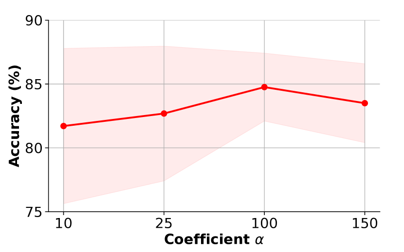
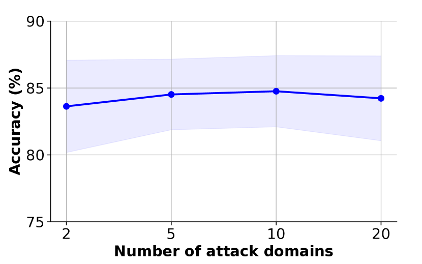
Figure 6: Hyperparameter analysis: The average accuracy of clean and attacked graphs, including Clean, nettack, PGD, TDGIA, and G-NIA.

D.5 Hyper-Parameter Analysis

We investigate the effects of coefficient $\alpha$ and the number of domains and compare the defense performance. Note that we take experimental results under evasion attacks on Cora as an illustration. Figure 6 shows that the average accuarcy of the clean and attacked graphs, along with the standard deviation of accuracy across these graphs, i.e., AVG in Section 4.1. For coefficient $\alpha$, we observe that when $\alpha$ is increasing, IDEA achieves better performance (higher accuracy), and performs more stable (lower standard deviation), validating the effectiveness of invariance component. While, too large $\alpha$ (e.g. $\alpha=150$) causes domination of invariance goal, leading to little attention to the predictive goal and degradation of performance. Regarding the number of attack domains, performance improves with increasing domain numbers, reaching its peak at 10 domains. This may be due to the relatively small number of nodes in the Cora dataset, suggesting that a larger number of domains (e.g., 20) is not necessary. In our main experiment shown in Table 1 (main body), we utilized $\alpha=100$ and the attack domain number = 10 to achieve the best results.

References

- [1] A. A. Alemi, I. Fischer, J. V. Dillon, and K. Murphy. Deep variational information bottleneck. In International Conference on Learning Representations, ICLR ’17, Oct. 2017.
- [2] M. Arjovsky, L. Bottou, I. Gulrajani, and D. Lopez-Paz. Invariant risk minimization. arXiv preprint arXiv:1907.02893, 2019.
- [3] A. Bojchevski and S. Günnemann. Adversarial attacks on node embeddings via graph poisoning. In Proceedings of the 36th International Conference on Machine Learning, ICML ’19, pages 695–704, 2019.
- [4] A. Bojchevski and S. Günnemann. Certifiable robustness to graph perturbations. In Advances in Neural Information Processing Systems 32, NeurIPS ’19, pages 8319–8330. 2019.
- [5] A. Bojchevski and S. Günnemann. Certifiable robustness to graph perturbations. NeurIPS ’19, pages 8317–8328, 2019.
- [6] A. Bojchevski, J. Klicpera, and S. Günnemann. Efficient robustness certificates for discrete data: Sparsity-aware randomized smoothing for graphs, images and more. In Proceedings of the 37th International Conference on Machine Learning, ICML ’20, pages 11647–11657, 2020.
- [7] Q. Cao, H. Shen, J. Gao, B. Wei, and X. Cheng. Popularity prediction on social platforms with coupled graph neural networks. In Proceedings of the 13th International Conference on Web Search and Data Mining, WSDM ’20, pages 70–78, 2020.
- [8] L. Chen, J. Li, J. Peng, T. Xie, Z. Cao, K. Xu, X. He, and Z. Zheng. A survey of adversarial learning on graphs. ArXiv, abs/2003.05730, 2020.
- [9] Y. Chen, R. Xiong, Z. Ma, and Y. Lan. When does group invariant learning survive spurious correlations? In Advances in Neural Information Processing Systems 36, NeurIPS ’22, 2022.
- [10] Y. Chen, H. Yang, Y. Zhang, M. KAILI, T. Liu, B. Han, and J. Cheng. Understanding and improving graph injection attack by promoting unnoticeability. In International Conference on Learning Representations, 2022.
- [11] Y. Chen, Y. Zhang, Y. Bian, H. Yang, M. KAILI, B. Xie, T. Liu, B. Han, and J. Cheng. Learning causally invariant representations for out-of-distribution generalization on graphs. In Advances in Neural Information Processing Systems 36, NeurIPS ’22, 2022.
- [12] D. Cheng, X. Wang, Y. Zhang, and L. Zhang. Graph neural network for fraud detection via spatial-temporal attention. IEEE Transactions on Knowledge and Data Engineering, 34(8):3800–3813, 2022.
- [13] P. Cheng, W. Hao, S. Dai, J. Liu, Z. Gan, and L. Carin. Club: A contrastive log-ratio upper bound of mutual information. In Proceedings of the 37th International Conference on Machine Learning, ICML ’20, 2020.
- [14] E. Creager, J.-H. Jacobsen, and R. Zemel. Environment inference for invariant learning. In Proceedings of the 38th International Conference on Machine Learning, ICML ’21, pages 2189–2200, 2021.
- [15] H. Dai, H. Li, T. Tian, X. Huang, L. Wang, J. Zhu, and L. Song. Adversarial attack on graph structured data. In Proceedings of the 35th International Conference on Machine Learning, ICML ’18, pages 1123–1132, 2018.
- [16] Q. Dai, X. Shen, L. Zhang, Q. Li, and D. Wang. Adversarial training methods for network embedding. In Proceedings of The Web Conference 2019, WWW ’19, pages 329–339, 2019.
- [17] N. Entezari, S. A. Al-Sayouri, A. Darvishzadeh, and E. E. Papalexakis. All you need is low (rank): Defending against adversarial attacks on graphs. In Proceedings of the 13th International Conference on Web Search and Data Mining, WSDM ’20, pages 169–177, 2020.
- [18] W. Fan, Y. Ma, Q. Li, Y. He, E. Zhao, J. Tang, and D. Yin. Graph neural networks for social recommendation. In The World Wide Web Conference, WWW ’19, pages 417–426, 2019.
- [19] F. Feng, X. He, J. Tang, and T.-S. Chua. Graph adversarial training: Dynamically regularizing based on graph structure. IEEE Transactions on Knowledge and Data Engineering, 2019.
- [20] L. Gosch, D. Sturm, S. Geisler, and S. Günnemann. Revisiting robustness in graph machine learning. In International Conference on Learning Representations, ICLR ’23, 2023.
- [21] W. Hamilton, Z. Ying, and J. Leskovec. Inductive representation learning on large graphs. NeurIPS ’17, pages 1024–1034, 2017.
- [22] W. Hu, M. Fey, M. Zitnik, Y. Dong, H. Ren, B. Liu, M. Catasta, and J. Leskovec. Open graph benchmark: Datasets for machine learning on graphs. Advances in neural information processing systems, pages 22118–22133, 2020.
- [23] W. Jin, T. Derr, Y. Wang, Y. Ma, Z. Liu, and J. Tang. Node similarity preserving graph convolutional networks. In Proceedings of the 14th International Conference on Web Search and Data Mining, WSDM ’21, pages 148–156, 2021.
- [24] W. Jin, Y. Li, H. Xu, Y. Wang, and J. Tang. Adversarial attacks and defenses on graphs: A review and empirical study. ArXiv, abs/2003.00653, 2020.
- [25] W. Jin, Y. Ma, X. Liu, X.-F. Tang, S. Wang, and J. Tang. Graph structure learning for robust graph neural networks. In Proceedings of the 26th ACM SIGKDD International Conference on Knowledge Discovery & Data Mining, KDD ’20, 2020.
- [26] D. P. Kingma and M. Welling. Auto-encoding variational bayes. In International Conference on Learning Representations, ICLR ’14, Oct. 2014.
- [27] T. N. Kipf and M. Welling. Semi-supervised classification with graph convolutional networks. In International Conference on Learning Representations, ICLR ’17, 2017.
- [28] K. Kong, G. Li, M. Ding, Z. Wu, C. Zhu, B. Ghanem, G. Taylor, and T. Goldstein. Robust optimization as data augmentation for large-scale graphs. In Proceedings of the IEEE conference on computer vision and pattern recognition, CVPR’22, 2022.
- [29] D. Krueger, E. Caballero, J.-H. Jacobsen, A. Zhang, J. Binas, D. Zhang, R. Le Priol, and A. Courville. Out-of-distribution generalization via risk extrapolation (rex). In Proceedings of the 38th International Conference on Machine Learning, ICML ’21, pages 5815–5826, 2021.
- [30] R. Lei, W. Zhen, Y. Li, B. Ding, and Z. Wei. Evennet: Ignoring odd-hop neighbors improves robustness of graph neural networks. In Advances in Neural Information Processing Systems 35, NeurIPS ’22, 2022.
- [31] B. Li, Y. Shen, Y. Wang, W. Zhu, D. Li, K. Keutzer, and H. Zhao. Invariant information bottleneck for domain generalization. In Proceedings of the 36th AAAI Conference on Artificial Intelligence, AAAI ’22, pages 7399–7407, 2022.
- [32] J. Li, J. Peng, L. Chen, Z. Zheng, T. Liang, and Q. Ling. Spectral adversarial training for robust graph neural network. IEEE Transactions on Knowledge and Data Engineering, 2022.
- [33] K. Li, Y. Liu, X. Ao, J. Chi, J. Feng, H. Yang, and Q. He. Reliable representations make a stronger defender: Unsupervised structure refinement for robust gnn. In Proceedings of the 28th ACM SIGKDD International Conference on Knowledge Discovery & Data Mining, KDD ’22, pages 925–935, 2022.
- [34] K. Li, Y. Liu, X. Ao, and Q. He. Revisiting graph adversarial attack and defense from a data distribution perspective. In International Conference on Learning Representations, ICLR ’23, 2023.
- [35] Y. Li, W. Jin, H. Xu, and J. Tang. Deeprobust: A pytorch library for adversarial attacks and defenses. In Proceedings of the 35rd AAAI Conference on Artificial Intelligence, AAAI ’21, 2021.
- [36] X. Lin, C. Zhou, H. Yang, J. Wu, H. Wang, Y. Cao, and B. Wang. Exploratory adversarial attacks on graph neural networks. 2020 IEEE International Conference on Data Mining (ICDM), pages 1136–1141, 2020.
- [37] X. Liu, W. Jin, Y. Ma, Y. Li, H. Liu, Y. Wang, M. Yan, and J. Tang. Elastic graph neural networks. In Proceedings of the 38th International Conference on Machine Learning, ICML ’21, pages 6837–6849, 2021.
- [38] X. Ma, J. Wu, S. Xue, J. Yang, C. Zhou, Q. Z. Sheng, H. Xiong, and L. Akoglu. A comprehensive survey on graph anomaly detection with deep learning. IEEE Transactions on Knowledge and Data Engineering, pages 1–1, 2021.
- [39] A. Madry, A. Makelov, L. Schmidt, D. Tsipras, and A. Vladu. Towards deep learning models resistant to adversarial attacks. In International Conference on Learning Representations, ICLR ’18, 2018.
- [40] F. Mujkanovic, S. Geisler, S. Günnemann, and A. Bojchevski. Are defenses for graph neural networks robust? In Advances in Neural Information Processing Systems 35, NeurIPS ’22, 2022.
- [41] J. Pearl. Causal inference in statistics: An overview. 2009.
- [42] J. Pearl. Causal inference. In Causality: Objectives and Assessment (NIPS 2008 Workshop), pages 39–58, 2010.
- [43] Q. Ren, Y. Chen, Y. Mo, Q. Wu, and J. Yan. Dice: Domain-attack invariant causal learning for improved data privacy protection and adversarial robustness. In Proceedings of the 28th ACM SIGKDD International Conference on Knowledge Discovery & Data Mining, KDD ’22, pages 1483–1492, 2022.
- [44] E. Rosenfeld, P. K. Ravikumar, and A. Risteski. The risks of invariant risk minimization. In International Conference on Learning Representations, ICLR ’21, 2021.
- [45] Y. Scholten, J. Schuchardt, S. Geisler, A. Bojchevski, and S. Günnemann. Randomized message-interception smoothing: Gray-box certificates for graph neural networks. In Advances in Neural Information Processing Systems 35, NeurIPS ’22, 2022.
- [46] Z. Shen, J. Liu, Y. He, X. Zhang, R. Xu, H. Yu, and P. Cui. Towards out-of-distribution generalization: A survey. arXiv preprint arXiv:2108.13624, 2021.
- [47] L. Sun, J. Wang, P. S. Yu, and B. Li. Adversarial attack and defense on graph data: A survey. ArXiv, abs/1812.10528, 2018.
- [48] Y. Sun, S. Wang, X.-F. Tang, T.-Y. Hsieh, and V. G. Honavar. Adversarial attacks on graph neural networks via node injections: A hierarchical reinforcement learning approach. In Proceedings of The Web Conference 2020, WWW ’20, pages 673–683, 2020.
- [49] S. Tao, Q. Cao, H. Shen, J. Huang, Y. Wu, and X. Cheng. Single node injection attack against graph neural networks. In Proceedings of the 30th ACM International Conference on Information and Knowledge Management, CIKM ’21, page 1794–1803, 2021.
- [50] S. Tao, Q. Cao, H. Shen, Y. Wu, L. Hou, F. Sun, and X. Cheng. Adversarial camouflage for node injection attack on graphs. ArXiv, abs/2208.01819, 2022.
- [51] S. Tao, H. Shen, Q. Cao, L. Hou, and X. Cheng. Adversarial immunization for certifiable robustness on graphs. In Proceedings of the 14th ACM International Conference on Web Search and Data Mining, WSDM’21, 2021.
- [52] L. Van der Maaten and G. Hinton. Visualizing data using t-sne. Journal of machine learning research, 9(11), 2008.
- [53] P. Veličković, G. Cucurull, A. Casanova, A. Romero, P. Liò, and Y. Bengio. Graph Attention Networks. In International Conference on Learning Representations, ICLR ’18, 2018.
- [54] J. Wang, M. Luo, F. Suya, J. Li, Z. Yang, and Q. Zheng. Scalable attack on graph data by injecting vicious nodes. arXiv preprint arXiv:2004.13825, 2020.
- [55] K. Wang, Z. Shen, C. Huang, C.-H. Wu, Y. Dong, and A. Kanakia. Microsoft academic graph: When experts are not enough. Quantitative Science Studies, 1(1):396–413, 2020.
- [56] H. Wu, C. Wang, Y. Tyshetskiy, A. Docherty, K. Lu, and L. Zhu. Adversarial examples on graph data: Deep insights into attack and defense. In Proceedings of the 28th International Joint Conference on Artificial Intelligence, IJCAI ’19, pages 4816–4823, 2019.
- [57] Q. Wu, H. Zhang, J. Yan, and D. Wipf. Handling distribution shifts on graphs: An invariance perspective. In International Conference on Learning Representations, ICLR ’22, 2022.
- [58] B. Xu, H. Shen, Q. Cao, K. Cen, and X. Cheng. Graph convolutional networks using heat kernel for semi-supervised learning. In Proceedings of the 28th International Joint Conference on Artificial Intelligence, IJCAI ’19, pages 1928–1934, 2019.
- [59] B. Xu, H. Shen, Q. Cao, Y. Qiu, and X. Cheng. Graph wavelet neural network. In International Conference on Learning Representations, ICLR ’19, 2019.
- [60] L. Yong, S. Zhu, L. Tan, and P. Cui. Zin: When and how to learn invariance without environment partition? In Advances in Neural Information Processing Systems 36, NeurIPS ’22, 2022.
- [61] H. Zeng, H. Zhou, A. Srivastava, R. Kannan, and V. K. Prasanna. Graphsaint: Graph sampling based inductive learning method. In International Conference on Learning Representations, 2020.
- [62] C. Zhang, K. Mohan, and J. Pearl. Causal inference with non-iid data using linear graphical models. In Advances in Neural Information Processing Systems 36, NeurIPS ’22, 2022.
- [63] X. Zhang and M. Zitnik. Gnnguard: Defending graph neural networks against adversarial attacks. In Proceedings of Neural Information Processing Systems, NeurIPS ’20, pages 9263–9275, 2020.
- [64] Y. Zhang, M. Gong, T. Liu, G. Niu, X. Tian, B. Han, B. Schölkopf, and K. Zhang. Adversarial robustness through the lens of causality. In International Conference on Learning Representations, ICLR ’22, 2022.
- [65] D. Zhu, Z. Zhang, P. Cui, and W. Zhu. Robust graph convolutional networks against adversarial attacks. In Proceedings of the 25th ACM SIGKDD International Conference on Knowledge Discovery & Data Mining, KDD ’19, pages 1399–1407, 2019.
- [66] X. Zou, Q. Zheng, Y. Dong, X. Guan, E. Kharlamov, J. Lu, and J. Tang. Tdgia: Effective injection attacks on graph neural networks. In Proceedings of the 27th ACM SIGKDD International Conference on Knowledge Discovery & Data Mining, page 2461–2471, 2021.
- [67] D. Zügner, A. Akbarnejad, and S. Günnemann. Adversarial attacks on neural networks for graph data. In Proceedings of the 24th ACM SIGKDD International Conference on Knowledge Discovery & Data Mining, KDD ’18, pages 2847–2856, 2018.
- [68] D. Zügner and S. Günnemann. Adversarial attacks on graph neural networks via meta learning. In International Conference on Learning Representations, ICLR ’19, 2019.
- [69] D. Zügner and S. Günnemann. Certifiable robustness and robust training for graph convolutional networks. In Proceedings of the 25th ACM SIGKDD International Conference on Knowledge Discovery & Data Mining, KDD ’19, pages 246–256, 2019.
- [70] D. Zügner and S. Günnemann. Certifiable robustness of graph convolutional networks under structure perturbations. In Proceedings of the 26th ACM SIGKDD International Conference on Knowledge Discovery & Data Mining, KDD ’20, 2020.