DP-LDMs: Differentially Private Latent
Diffusion Models

Abstract

Diffusion models (DMs) are widely used for generating high-quality high-dimensional images in a non-differentially private manner. However, due to the notoriously slow training process of DMs, applying differential privacy (DP) to the training routine requires adding large amounts of noise, yielding poor-quality generated images. To address this challenge, recent papers suggest pre-training DMs with public data, then fine-tuning them with private data using DP-SGD for a relatively short period. In this paper, we further improve the current state of DMs with DP by adopting the Latent Diffusion Models (LDMs). LDMs are equipped with powerful pre-trained autoencoders that map the high-dimensional pixels into lower-dimensional latent representations, in which DMs are trained, yielding a more efficient and fast training of DMs. In our algorithm, DP-LDMs, rather than fine-tuning the entire DMs, we fine-tune only the attention modules of LDMs at varying layers with privacy-sensitive data, reducing the number of trainable parameters by roughly $90\%$ and achieving a better accuracy, compared to fine-tuning the entire DMs. The smaller parameter space to fine-tune with DP-SGD helps our algorithm to achieve new state-of-the-art results in several public-private benchmark data pairs. Our approach also allows us to generate more realistic, high-dimensional images (256x256) and those conditioned on text prompts with differential privacy, which have not been attempted before us, to the best of our knowledge. Our approach provides a promising direction for training more powerful, yet training-efficient differentially private DMs, producing high-quality high-dimensional DP images.

1 Introduction

Creating impactful machine learning solutions for real-world applications often requires access to personal data that may compromise privacy, raising ethical and legal concerns. These reasons motivate differentially private data generation as an active area of research. The main objective of this research is to generate synthetic data that preserves the privacy of the individuals in the original data while maintaining the statistical properties of the original data. Unlike traditional methods that require strict assumptions about the intended use of synthetic data (Mohammed et al., 2011; Xiao et al., 2010; Hardt et al., 2012; Zhu et al., 2017), recent approaches aim to create synthetic data that is general-purpose and useful for a range of downstream tasks, including training a classifier and performing statistical testing. These popular approaches include GAN-based models (Xie et al., 2018; Torkzadehmahani et al., 2019; Yoon et al., 2019; Chen et al., 2020), optimal transport or kernel-based distance approaches (Cao et al., 2021; Harder et al., 2021; Vinaroz et al., 2022; Yang et al., 2023), and diffusion models (Dockhorn et al., 2023; Ghalebikesabi et al., 2023).

Many of these popular approaches for differentially private data generation operate on small generative models, such as two-layer convolutional neural networks (CNNs), and simple datasets such as MNIST and FashionMNIST. This is because the DP training algorithm, called differentially private stochastic gradient descent (DP-SGD) by Abadi et al. (2016), does not scale well for large models that are necessary for learning complex distributions. For instance, the recent approach by Dockhorn et al. (2023) uses diffusion models that have shown impressive performance on high-dimensional image generation in non-DP settings. However, due to the scalability issue of DP-SGD, DP trained diffusion models yield rather underwhelming performance when evaluated on complex datasets such as CIFAR10 and CelebA.

More recent approaches attempt to overcome this issue by utilizing the abundant resource of public data. For example, Harder et al. (2023) use public data for pre-training a large feature extractor model to learn useful features without incurring a privacy loss, then use those features to train a generator using private data. As another example, Ghalebikesabi et al. (2023) pretrain a large diffusion-based generator using public data, then fine-tune it for private data for a relatively small number of epochs using DP-SGD. This method currently achieves the state-of-the-art performance on CIFAR10 image generation using DMs with differential privacy.

In this paper, we attempt to further improve the performance of differentially private image generation by reducing the number of parameters to fine-tune. To achieve this, we build off of latent diffusion models (LDMs) by Rombach et al. (2022), which uses a pre-trained autoencoder to reduce the size of images, often called latent variables, entering into the diffusion model. This latent diffusion model defined on this latent space has a significantly lower number of parameters than the diffusion model defined on the pixel space. Inspired by You & Zhao (2023) that establishes a transfer learning paradigm for LDMs in non-DP settings, we pre-train the entire LDM including the auto-encoder using public data, and fine-tune only attention modules and a conditioning embedder using our private data. As a result, the number of trainable parameters under our approach is only $10\%$ of that of the diffusion models used in (Ghalebikesabi et al., 2023) and achieves better performance.

While readers might find the use of DP-SGD to fine-tune a pre-trained model unremarkable at first glance, the potential impact of this seemingly ordinary method is substantial. We describe the significance in the following:

• We improve the state-of-the-art (SOTA) results in all three commonly used image benchmark datasets in DP literature, including CIFAR10, CelebA64, and MNIST. This is thanks to the unique aspects of our proposed method, i.e., training DMs in the latent space and fine-tuning only a few selected parameters. This makes our training process considerably more efficient than training a DM from scratch with DP-SGD in (Dockhorn et al., 2023), or fine-tuning the entire DM with DP-SGD in (Ghalebikesabi et al., 2023). Reducing the fine-tuning space not only improves the performance but also helps to democratize DP image generation using diffusion models, which otherwise have to rely on massive computational resources only available to a small fraction of the field and would leave a huge carbon footprint (e.g., reducing the training time from 192 GPU hours Dockhorn et al. (2023) to mere 10 GPU hours for similar performance).

• We push the boundary of what DP-SGD fine-tuned generative models can achieve, by being the first to produce high-dimensional images (256x256) at a reasonable privacy level. We showcase this in text-conditioned and class-conditioned image generation, where we input a certain text prompt (or a class label) and generate a corresponding image from a DP-fine-tuned LDM for CelebAHQ. These conditional, high-dimensional image generation tasks present more complex but also more realistic benchmarks compared to the conventional CIFAR10 and MNIST datasets. These latter datasets, though widely used in DP image generation literature for years, are now rather simplistic and outdated. Our work contributes to narrowing down the large gap between the current state of synthetic image generation in non-DP settings and that in DP settings.

In the following section, we provide relevant background information. We then present our method along with related work and experiments on benchmark datasets.

2 Background

We first describe latent diffusion models (LDMs), then the definition of differential privacy (DP) and finally the DP-SGD algorithm, which we will use to train the LDM in our method.

2.1 Latent Diffusion Models (LDMs)

Latent diffusion models (LDMs) by Rombach et al. (2022) are a modification of denoising diffusion probabilistic models (DDPMs) by Ho et al. (2020) in the following way. First, Rombach et al. (2022) uses a powerful auto-encoder, consisting of an encoder $\Delta$ and a decoder $\nabla$. The encoder transforms a high-dimensional pixel representation $\mathbf{x}$ into a lower-dimensional latent representation $\mathbf{z}$ via $\mathbf{z}=\Delta(\mathbf{x})$; and the decoder transforms the lower-dimensional latent representation back to the original space via $\hat{\mathbf{x}}=\nabla(\mathbf{z})$. Rombach et al. (2022) use a combination of a perceptual loss and a patch-based adversarial objective, with extra regularization for better-controlled variance in the learned latent space, to obtain powerful autoencoders (See section 3 in (Rombach et al., 2022) for details). This training loss encourages the latent representations to carry equivalent information (e.g., the spatial structure of pixels) as the pixel representations, although the dimensionality of the former is greatly reduced.

Second, equipped with the powerful auto-encoder, Rombach et al. (2022) trains a diffusion model (typically a UNet) in the latent representation space. Training a DM in this space can significantly expedite the training process of diffusion models, e.g., from hundreds of GPU days to several GPU hours for similar accuracy.

Third, LDMs also contain attention modules that take inputs from a conditioning embedder, inserted into the layers of the underlying UNet backbone to achieve flexible conditional image generation (e.g., generating images conditioning on text, image layout, class labels, etc.). The modified Unet is then used as a function approximator $\tau_{\mathbf{\bm{\theta}}}$ to predict an initial noise from the noisy lower-dimensional latent representations at several finite time steps $t$, where in LDMs, the noisy representations (rather than data) follow the diffusion process defined in Ho et al. (2020).

The parameters of the approximator are denoted by $\mathbf{\bm{\theta}}=[\mathbf{\bm{\theta}}^{U},\mathbf{\bm{\theta}}^{Att},\mathbf{\bm{\theta}}^{Cn}]$, where $\mathbf{\bm{\theta}}^{U}$ are the parameters of the underlying Unet backbone, $\mathbf{\bm{\theta}}^{Att}$ are the parameters of the attention modules, and $\mathbf{\bm{\theta}}^{Cn}$ are the parameters of the conditioning embedder (We will explain these further in Sec. 3). These parameters are then optimized by minimizing the prediction error defined by

$$\mathcal{L}_{ldm}(\mathbf{\bm{\theta}})=\mathbb{E}_{(\mathbf{z}_{t},y),\tau,t}\left[\|\tau-\tau_{\mathbf{\bm{\theta}}}(\mathbf{z}_{t},t,y)\|_{2}^{2}\right],$$ (1)

where $\tau\sim\mathcal{N}(0,I),\mathbf{z}_{t}=\Delta(\mathbf{x}_{t})$ and $y$ is what the model is conditioning on to generate data, e.g., class labels, or a prompt. Once the approximator is trained, the drawn samples in latent space, $\tilde{\mathbf{z}}$, are transformed back to pixel space through the decoder, i.e., $\tilde{\mathbf{x}}=\nabla(\tilde{\mathbf{z}})$. Our work introduced in Sec. 3 pre-trains both auto-encoder and $\tau_{\mathbf{\bm{\theta}}}$ using public data, then fine-tunes only $\mathbf{\bm{\theta}}_{Att},\mathbf{\bm{\theta}}_{Cn}$, the parameters of the attention modules and the conditioning embedder, using DP-SGD for private data.

2.2 Differential Privacy (DP)

A mechanism $\mathcal{M}$ is ($\epsilon$, $\delta$)-DP for a given $\epsilon\geq 0$ and $\delta\geq 0$ if and only if $\text{Pr}[\mathcal{M}(\mathcal{D})\in S]\leq e^{\epsilon}\cdot\text{Pr}[\mathcal{M}(\mathcal{D}^{\prime})\in S]+\delta$ for all possible sets of the mechanism’s outputs $S$ and all neighbouring datasets $\mathcal{D}$, $\mathcal{D}^{\prime}$ that differ by a single entry. A single entry difference could come from either replacing or removing one entry from the dataset $\mathcal{D}$. One of the most well-known and widely used DP mechanisms is the Gaussian mechanism. The Gaussian mechanism adds a calibrated level of noise to a function $\mu:\mathcal{D}\mapsto\mathbb{R}^{p}$ to ensure that the output of the mechanism is ($\epsilon,\delta$)-DP: $\widetilde{\mu}(\mathcal{D})=\mu(\mathcal{D})+n$, where $n\sim\mathcal{N}(0,\sigma^{2}\Delta_{\mu}^{2}\mathbf{I}_{p})$. Here, $\sigma$ is often called a privacy parameter, which is a function of $\epsilon$ and $\delta$. $\Delta_{\mu}$ is often called the global sensitivity (Dwork et al., 2006), which is the maximum difference in $L_{2}$-norm given two neighbouring $\mathcal{D}$ and $\mathcal{D}^{\prime}$, $||\mu(\mathcal{D})-\mu(\mathcal{D}^{\prime})||_{2}$. Because we are adding noise, the natural consequence is that the released function $\tilde{\mu}(\mathcal{D})$ is less accurate than the non-DP counterpart, $\mu(\mathcal{D})$. This introduces privacy-accuracy trade-offs.

Two properties of DP: The post-processing invariance property of DP (Dwork et al., 2006) implies that the composition of any data-independent mapping with an $(\epsilon,\delta)$-DP algorithm is also $(\epsilon,\delta)$-DP. So no analysis of the released synthetic data can yield more information about the real data than what our choice of $\epsilon$ and $\delta$ allows. The composability property Dwork et al. (2006) states that the strength of privacy guarantee degrades in a measurable way with repeated use of DP-algorithms. This composability property of DP poses a significant challenge in deep learning.

DP-SGD (Abadi et al., 2016) is one of the most widely used DP algorithms for training deep neural network models. It modifies stochastic gradient descent (SGD) by adding an appropriate amount of noise by employing the Gaussian mechanism to the gradients in every training step to ensure the parameters of a neural network are differentially private. However, there are two challenges in DP-SGD. First, it is infeasible to obtain an analytic sensitivity of gradients under complex deep neural network models. A remedy to this issue is explicitly normalizing the norm of each sample-wise gradient with some pre-chosen value $C$ such that the gradient norm given any datapoint’s difference between two neighbouring datasets cannot exceed $C$. Second, due to the composability property of DP, privacy loss is accumulating over a typically long course of training. Abadi et al. (2016) exploit the subsampled Gaussian mechanism (i.e., applying the Gaussian mechanism on randomly subsampled data) to achieve a tight privacy bound. The Opacus package (Yousefpour et al., 2021) implements the privacy analysis in DP-SGD, which we adopt in our method.

3 Differentially private latent diffusion models (DP-LDMs)

In our method, which we call differentially private latent diffusion models (DP-LDMs), we carry out two training steps: non-private and private steps.

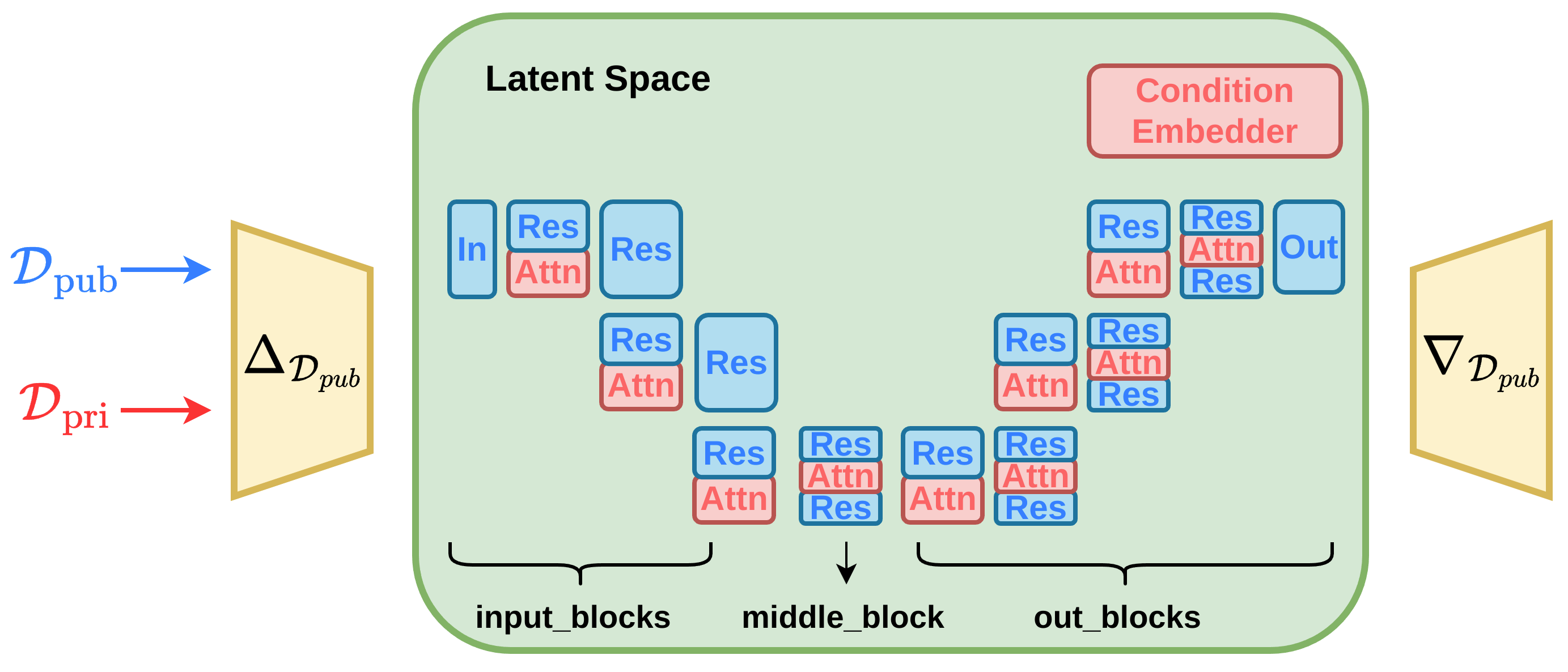
Figure 1: A schematic of DP-LDM. In the non-private step, we pre-train the auto-encoder depicted in yellow (Right and Left) with public data. We then forward pass the public data through the encoder (blue arrow on the left) to obtain latent representations. We then train the diffusion model (depicted in the green box) on the lower-dimensional latent representations. The diffusion model consists of the Unet backbone and added attention modules (in Red) with a conditioning embedder (in Red, at top-right corner). In the private step, we forward pass the private data (red arrow on the left) through the encoder to obtain latent representations of the private data. We then fine-tune only the red blocks, which are attention modules and conditioning embedder, with DP-SGD. Once the training is done, we sample the latent representations from the diffusion model, and pass them through the decoder to obtain the image samples in the pixel space.

Non-Private Step: Pre-training an autoencoder and a DM using public data.

Following Rombach et al. (2022), we first pre-train an auto-encoder. The encoder scales down an image $\mathbf{x}\in\mathbb{R}^{H\times W\times 3}$ to a 3-dimensional latent representation $\mathbf{z}\in\mathbb{R}^{h\times w\times c}$ by a factor of $f$, where $f=H/h=W/w$. This 3-dimensional latent representation is chosen to take advantage of image-specific inductive biases that the Unet contains, e.g., 2D convolutional layers. Following Rombach et al. (2022), we also train the autoencoder by minimizing a combination of different losses, such as perceptual loss and adversarial loss, with some form of regularization. See Appendix Sec. A.1 for details. As noted by Rombach et al. (2022), we also observe that a mild form of downsampling performs the best, achieving a good balance between training efficiency and perceptually decent results. See Appendix Sec. A.1 for details on different scaling factors $f=2^{m}$, with a different value of $m$. Training an auto-encoder does not incur any privacy loss, as we use public data $\mathcal{D}_{pub}$ that is similar to private data $\mathcal{D}_{priv}$ at hand. The trained autoencoder is, therefore, a function of public data: an encoder $\Delta_{\mathcal{D}_{pub}}$ and a decoder $\nabla_{\mathcal{D}_{pub}}$.

A forward pass through the trained encoder $\Delta_{\mathcal{D}_{pub}}$ gives us a latent representation of each image, which we use to train a diffusion model. As in (Rombach et al., 2022), we consider a modified Unet for the function approximator $\tau_{\mathbf{\bm{\theta}}}$ shown in Fig. 1. We minimize the loss given in (1) to estimate the parameters of $\tau_{\mathbf{\bm{\theta}}}$ as:

$$\mathbf{\bm{\theta}}^{U}_{\mathcal{D}_{pub}},\mathbf{\bm{\theta}}^{Att}_{\mathcal{D}_{pub}},\mathbf{\bm{\theta}}^{Cn}_{\mathcal{D}_{pub}} =\mathop{\rm arg\,min}_{\mathbf{\bm{\theta}}}\;\mathcal{L}_{ldm}(\mathbf{\bm{\theta}}).$$ (2)

Since we use public data, there is no privacy loss incurred in estimating the parameters, which are a function of public data $\mathcal{D}_{pub}$.

Private Step: Fine-tuning attention modules & conditioning embedder for private data.

Given a pre-trained diffusion model, we fine-tune the attention modules and a conditioning embedder using our private data.

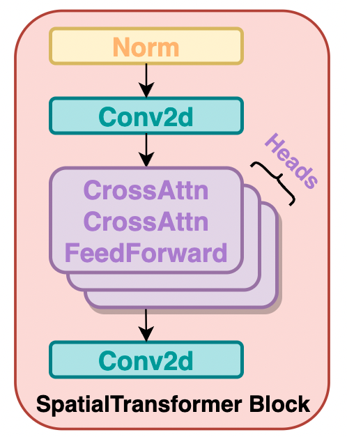
Figure 2: A SpatialTransformer Block

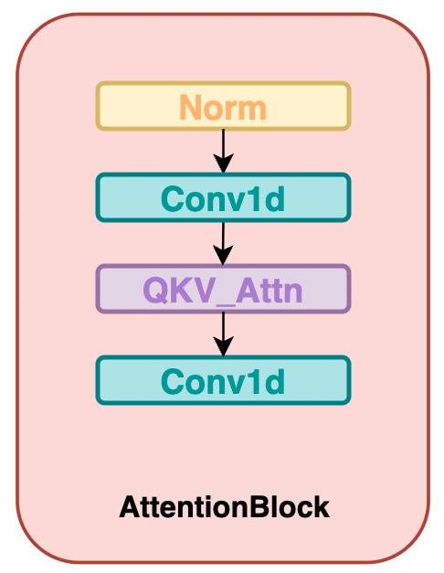
Figure 3: An AttentionBlock

For the models with the conditioned generation, the attention modules refer to the spatial transformer blocks shown in Fig. 2 which contains cross-attentions and multiple heads. For the models with an unconditional generation, the attention modules refer to the attention blocks shown in Fig. 3. Consequently, the parameters of the attention modules, denoted by $\mathbf{\bm{\theta}}^{Att}$, differ, depending on the conditioned or unconditioned cases. The conditioning embedder only exists in the conditioned case. Depending on the different modalities the model is trained on, the conditioning embedder takes a different form. For instance, if the model generates images conditioning on the class labels, the conditioning embedder is simply a class embedder, which embeds class labels to a latent dimension. If the model conditions on language prompts, the embedder can be a transformer.

The core part of the spatial transformer block and the attention block is the attention layer, which has the following parameterization (For simplicity, we explain it under the conditioned case):

$$\text{Attention}(\psi_{i}(\mathbf{z}_{t}),\phi(y);Q,K,V) =\text{softmax}\left(\tfrac{QK^{T}}{\sqrt{d_{k}}}\right)V\;\in\mathbb{R}^{N\times d_{k}},$$ (3)

where $\psi_{i}(\mathbf{z}_{t})\in\mathbb{R}^{N\times d^{i}}$ is an intermediate representation of the latent representation $\mathbf{z}_{t}$ through the $i$th residual convolutional block in the backbone Unet, and $\phi(y)\in\mathbb{R}^{M\times d_{c}}$ is the embedding of what the generation is conditioned on (e.g., class labels, CLIP embedding). Furthermore, $Q=\psi_{i}(\mathbf{z}_{t})W_{Q}^{(i)}{{}^{\top}},K=\phi(\mathbf{x})W_{K}^{(i)}{{}^{\top}},$ and $V=\phi(\mathbf{x})W_{V}^{(i)}{{}^{\top}},$ where the parameters are denoted by $W_{Q}^{(i)}\in\mathbb{R}^{d_{k}\times d^{i}}$; $W_{K}^{(i)}\in\mathbb{R}^{d_{k}\times d_{c}}$; and $W_{V}^{(i)}\in\mathbb{R}^{d_{k}\times d_{c}}$. Unlike the conditioned case, where the key ($K$) and value ($V$) vectors are computed as a projection of the conditioning embedder, the key and value vectors are a projection of the pixel embedding $\psi_{i}(\mathbf{z}_{t})$ only in the case of the unconditioned model. We run DP-SGD to fine-tune these parameters to obtain differentially private $\mathbf{\bm{\theta}}^{Att}_{\mathcal{D}_{priv}}$ and $\mathbf{\bm{\theta}}^{Cn}_{\mathcal{D}_{priv}}$, starting from $\mathbf{\bm{\theta}}^{Att}_{\mathcal{D}_{pub}},\mathbf{\bm{\theta}}^{Cn}_{\mathcal{D}_{pub}}$. Our algorithm is given in Algorithm 1.

Algorithm 1 DP-LDM

  Input: Latent representations through a pre-trained auto-encoder and conditions (if conditioned generation) $\{(\mathbf{z}_{i},y_{i})\}_{i=1}^{N}$, a pre-trained diffusion model with parameters $\mathbf{\bm{\theta}}$, number of iterations $P$, mini-batch size $B$, clipping norm $C$, learning rate $\eta$, privacy parameter $\sigma$ corresponding to ($\epsilon$, $\delta$)-DP. Denote $\hat{\mathbf{\bm{\theta}}}=\{\mathbf{\bm{\theta}}^{Att},\mathbf{\bm{\theta}}^{Cn}\}$

  for $p=1$ to $P$ do

     Step 1. Take a mini-batch $B_{p}$ uniformly at random with a sampling probability, $q=B/N$

     Step 2. For each sample $i\in B_{p}$ compute the gradient: $g_{p}(\mathbf{z}_{i},y_{i})=\nabla_{\hat{\mathbf{\bm{\theta}}}_{p}}\mathcal{L}_{ldm}(\hat{\mathbf{\bm{\theta}}}_{p},\mathbf{z}_{i},y_{i})$

     Step 3. Clip the gradient: $\hat{g}_{p}(\mathbf{z}_{i},y_{i})=g_{p}(\mathbf{z}_{i},y_{i})/\max(1,\|g_{p}(\mathbf{z}_{i},y_{i})\|_{2}/C)$

     Step 4. Add noise: $\tilde{g}_{p}=\frac{1}{B}\sum_{i=1}^{B}\hat{g}_{p}(\mathbf{z}_{i},y_{i})+\mathcal{N}(0,\sigma^{2}C^{2}I)$

     Step 5. Gradient descent: $\hat{\mathbf{\bm{\theta}}}_{p+1}=\hat{\mathbf{\bm{\theta}}}_{p}-\eta\tilde{g}_{p}$

  end for

  Return: ($\epsilon$, $\delta$)-differentially private $\hat{\mathbf{\bm{\theta}}}_{P}=\{\mathbf{\bm{\theta}}^{Att}_{P},\mathbf{\bm{\theta}}^{Cn}_{P}\}$

Why do we choose the attention modules to be fine-tuned among any other parts of the model?

Our rationale behind this choice is as follows. The output of the attention in (3) assigns a high focus to the features that are more important, by zooming into what truly matters in an image depending on a particular context, e.g., relevant to what the image is conditioned on. This can be quite different when we move from one distribution to the other. By fine-tuning the attention modules (together with the conditioning embedder when conditioned case), we are able to effectively transfer what we learned from the public data distribution to the private data distribution, as shown in Sec. 5. However, if we fine-tune other parts of the model, e.g., the ResBlocks, the fine-tuning of these blocks can make a large change in the features themselves, which could reduce the performance in the private training. See our results when fine-tuning other parts of the model in Sec. 5.

The idea of fine-tuning attention blocks is explored elsewhere. For instance, in fine-tuning large language models, existing work introduces a few new parameters to transformer attention blocks, and those new parameters are fine-tuned (Yu et al., 2022; Hu et al., 2021) to adapt to new distributions. In the context of pre-trained diffusion models, adding, modifying, and controlling attention layers are gaining popularity for tasks such as image editing and text-to-image generation(Hertz et al., 2022; Park et al., 2023; Zhang et al., 2023; You & Zhao, 2023).

Which public dataset do I use for a given private dataset?

This is an open question in transfer learning literature. Generally, if the two datasets are close to each other in some sense, they are assumed to be a better pair. We use FID as a proxy to judge the similarity between two image datasets. For instance, if a public dataset from the private dataset has a smaller FID than other candidates, we use that public data to begin with (See Sec. 5). In other datasets out of the image domain, there could be a more appropriate metric to use than FID, e.g., in the case of discrete data, kernel-based distance metrics with an appropriately chosen kernel could be more useful.

4 Related Work

Early efforts in differentially private data generation imposes strict limitations on the data type and the intended purpose of the released data (Snoke & Slavković, 2018; Mohammed et al., 2011; Xiao et al., 2010; Hardt et al., 2012; Zhu et al., 2017), which leads to the difficulties in generating large-scale data. Later, several works have explored generating discrete data with restricted range of values, by understanding the relationships of small groups of features and then privatizing them (Zhang et al., 2017; Qardaji et al., 2014; Chen et al., 2015; Zhang et al., 2021). However, these techniques cannot be applied to high-dimensional data due to the constraint of discretization. Recently, more efforts have focused on leveraging advanced generative models to achieve better differentially private synthetic data. Some of them (Xie et al., 2018; Torkzadehmahani et al., 2019; Frigerio et al., 2019; Yoon et al., 2019; Chen et al., 2020) utilize generative adversarial networks (GANS)(Goodfellow et al., 2014), or trained GANs with the PATE structure (Papernot et al., 2017). Other works have employed variational autoencoders (VAEs) (Acs et al., 2018; Jiang et al., 2022; Pfitzner & Arnrich, 2022), or proposed customized structures (Harder et al., 2021; Vinaroz et al., 2022; Cao et al., 2021; Liew et al., 2022a; Harder et al., 2023). For instance, Harder et al. (2023) pretrained perceptual features using public data and privatized only data-dependent terms using maximum mean discrepancy.

Limited works have so far delved into privatizing diffusion models. Dockhorn et al. (2023) develop a DP score-based generative models Song et al. (2021) using DP-SGD, applied to relatively simple datasets such as MNIST, FashionMNIST and CelebA (downsampled to 32$\times$32). Ghalebikesabi et al. (2023) fine-tune the ImageNet pre-trained diffusion model (DDPM) (Ho et al., 2020) with more than 80 M parameters using DP-SGD for CIFAR-10. We instead adopt a different model (LDM) and fine-tune only the small part of the DM in our model to achieve better privacy-accuracy trade-offs. As concurrent work to ours, Lin et al. (2023) propose an API-based approach that uses a DP-histogram mechanism to generate high-quality synthetic data. However, Lin et al. (2023) do privatize diffusion models directly, so we do not compare our method against it.

5 Experiments

Here, we demonstrate the performance of our method in comparison with the state-of-the-art methods in DP data generation, using several combinations of public/private data of different levels of complexity at varying privacy levels.

Datasets. For private datasets, we considered three image datasets of varying complexity : the commonly used datasets MNIST (LeCun & Cortes, 2010), the more complex datasets CelebA (Liu et al., 2015) , and also CIFAR-10 (Krizhevsky et al., 2009). In addition, we also consider the high-quality version CelebAHQ of size $256\times 256$ to generate high-dimensional images. For text-to-image generation, we used Multi-Modal-CelebAHQ (MM-CelebAHQ)(Xia et al., 2021) dataset, containing of 30,000 $256\times 256$ images, each of which is accompanied by descriptive text captions. As public datasets, we used EMNIST (Cohen et al., 2017) English letter split parts for MNIST, ImageNet (Deng et al., 2009) (rescaled it to the corresponding sizes) for CelebA and CIFAR-10 and CelebAHQ, and LAION-400M (Schuhmann et al., 2021) for MM-CelebAHQ.

Implementations. We implemented DP-LDMs in PyTorch Lightning (Paszke et al., 2019) building on the LDM codebase by Rombach et al. (2022) and Opacus (Yousefpour et al., 2021) for DP-SGD training. Several recent papers present the importance of using large batches in DP-SGD training to improve accuracy at a fixed privacy level (Ponomareva et al., 2023; De et al., 2022; Bu et al., 2022). To incorporate this finding in our work, we write custom batch splitting code that integrates with Opacus and Pytorch Lightning, allowing us to test arbitrary batch sizes. Our DP-LDM also improves significantly with large batches as will be shown soon, consistent with the findings in the recent work.

Evaluation. For the simple dataset MNIST, we take generated samples to train downstream classifiers and compute the accuracy on real data. We consider CNN classifier as in standard practice, and also Wide ResNet (WRN-40-4), a much larger classifier. For CelebA, CIFAR-10, CelebAHQ, and MM-CelebAHQ, we measure the model performance by computing the Fréchet Inception Distance (FID) (Heusel et al., 2017) between the generated samples and the real data. For CIFAR-10, we additionally train downstream classifiers (ResNet-9 and WRN-40-4) to compare against other state-of-the-art methods. Each number in our tables represents an average value across three independent runs, with a standard deviation (unless stated otherwise). Values for comparison methods are taken from their papers, with an exception for the DP-MEPF comparison to CelebAHQ, which we ran their code by loading this data.

5.1 Transferring from Imagenet to CIFAR10 distribution

Table 1: FID scores (lower is better) for synthetic CIFAR-10 data.

	$\epsilon=10$	$\epsilon=5$	$\epsilon=1$
DP-LDM	8.4 $\pm$ 0.2	13.4 $\pm$ 0.4	22.9 $\pm$ 0.5
DP-Diffusion	9.8	15.1	25.2
DP-MEPF $(\mathbf{\bm{\phi}}_{1},\mathbf{\bm{\phi}}_{2})$	29.1	30.0	54.0
DP-MEPF ($\mathbf{\bm{\phi}}_{1}$)	30.3	35.6	56.5

Table 2: Test accuracies (higher is better) of ResNet9 (left) and WRN40-4 (right) trained on CIFAR-10 synthetic data. When trained on real data, test accuracy is 88.3% on ResNet9.

	ResNet 9
	$\epsilon=10$	$\epsilon=5$	$\epsilon=1$
DP-LDM	65.3 $\pm$ 0.3	59.1 $\pm$ 0.2	51.3 $\pm$ 0.1
DP-MEPF ($\mathbf{\bm{\phi}}_{1},\mathbf{\bm{\phi}}_{2}$)	48.9	47.9	28.9
DP-MEPF ($\mathbf{\bm{\phi}}_{1}$)	51.0	48.5	29.4
DP-MERF	13.2	13.4	13.8

WRN40-4
	$\epsilon=10$
DP-LDM	78.6 $\pm$ 0.3
DP-Diffusion	75. 6

First, we pre-train a class-conditional LDM model considering ImageNet32 as public data. The Unet we use has 16 SpatialTransformer blocks as in Fig. 2. For the fine-tuning part, we consider CIFAR-10 as the private dataset and test the performance of DP-LDM at different privacy levels for 3 independent sampling runs. See Appendix Sec. A.3 for all experimental details.

Comparison to other SOTA methods in terms of FID (the lower the better) is given in Table  1. Our DP-LDM outperforms other methods at all epsilon levels ($\epsilon=1,5,10$ and $\delta=10^{-5}$). These FID values correspond to the case where only 9-16 attention modules are fine-tuned (i.e., fine-tuning only $10\%$ of trainable parameters in the model) and the rest remain fixed. See Table  10 for ablation experiments for fine-tuning different attention modules. In terms of downstream accuracy of ResNet-9 and WRN40-4 classifiers, DP-LDM also outperforms others, as shown in Table  2. Both classifiers are trained with 50K synthetic samples and then evaluated on real data samples.

Table 3: Fine-tuning different parts of the model for synthetic CIFAR-10 images.

	$\epsilon=1$
	Input block	Attention module
FID	50.2 $\pm$ 0.2	22.9 $\pm$ 0.5

	$\epsilon=10$
	Resblocks	Attention module
FID	86.9 $\pm$ 0.6	8.4 $\pm$ 0.2

When we fine-tune other parts of the model, we see a significant drop in accuracy as shown in Table  3. This confirms that fine-tuning resblocks or input blocks alone is less effective than fine-tuning attention modules at a fixed privacy budget.

5.2 Transferring from Imagenet to CelebA distribution

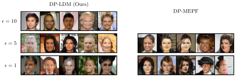
Figure 9: Synthetic $64\times 64$ CelebA samples generated at different levels of privacy. Samples for DP-MEPF are taken from Harder et al. (2023).

We evaluate the performance of our model on the task of unconditional image generation for CelebA (rescaled to 64x64) using an LDM pretrained on ImageNet. Additional experiments for CelebA32 are available in appendix A.4 We compare DP-LDM to existing methods at the privacy settings $\delta=10^{-6}$ and $\epsilon=1,5,10$ in Table 4. We achieve a new SOTA results at $\epsilon=10,5$ and are comparable to DP-MEPF at $\epsilon=1$. Samples are available in Figure 9. Table 5 provides evidence suggesting that training with larger batch sizes improves the performance of the model.

Table 4: CelebA FID scores (lower is better) for images of resolution $64\times 64$.

	$\epsilon=10$	$\epsilon=5$	$\epsilon=1$
DP-LDM (ours, average)	14.3 $\pm$ 0.1	16.1 $\pm$ 0.2	21.1 $\pm$ 0.2
DP-LDM (ours, best)	14.2	15.8	21.0
DP-MEPF $(\mathbf{\bm{\phi}}_{1})$	17.4	16.5	20.4
DP-GAN (pre-trained)	57.1	62.3	72.5

Table 5: Effect of increasing batch size on FID. At a fixed epsilon level, larger batches improve FIDs.

Batch size	$\epsilon=10$	$\epsilon=5$	$\epsilon=1$
$512$	$17.2\pm 0.1$	$18.0\pm 0.1$	$22.3\pm 0.2$
$2048$	$16.2\pm 0.2$	$17.1\pm 0.2$	$22.1\pm 0.1$
$8192$	$\textbf{14.3}\pm 0.1$	$\textbf{16.1}\pm 0.2$	$\textbf{21.1}\pm 0.2$

5.3 Transferring from EMNIST to MNIST distribution

To choose the public dataset for MNIST, we consider SVHN (Netzer et al., 2011), KMNIST (Clanuwat et al., 2018), and EMNIST (Cohen et al., 2017) as candidates. As a selection criterion, we computed the FID score between the samples from each candidate dataset and those from MNIST. Based on the FID scores (See Appendix Sec. A.2.1 for FIDs and additional experiments for SVHN and KMNIST), we chose EMNIST as the public dataset to pretrain a class-conditional LDM. We only took the English letter split of EMNIST such that the model does not see the MNIST data during the non-private pre-training step. We then finetune the attention modules with MNIST and test the performance of DP-LDM with downstream classifiers. We compare DP-LDM to existing methods with the most common DP settings $\epsilon=1,10$ and $\delta=10^{-5}$ in Table  7 in Appendix Sec. A.2. We also did ablation experiments to reduce the trainable parameters in Appendix Sec. A.2.2.

5.4 differentially private generation for high quality CelebA

With the latent representations of the inputs, LDMs can better improve DP training. We present high-dimensional differentially private generation for CelebAHQ in this section.

Text-to-image generation. For text-to-image generation, we fine-tune the LDM models pretrained with LAION-400M (Schuhmann et al., 2021) for MM-CelebAHQ (256 $\times$ 256). Each image is described by a caption, which is fed to the conditioning embedder, BERT (Devlin et al., 2018). We freeze the BERT embedder during fine-tuning to reduce the trainable parameters, then we bring back BERT for sampling. DP-LDM achieves FID scores of 44.5 for $\epsilon=10$ and 55.0 for $\epsilon=1$. We illustrate our samples with example prompts in Fig. 4. The samples are faithful to our input prompts even at the $\epsilon=1$ level.

	”This woman has brown hair, and	”This man has sideburns,	”She wears heavy makeup.
	black hair. She is attractive	and mustache.”	She is attractive and has
	and wears lipstick”		wavy hair, and black hair.”
$\epsilon=10$
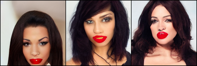
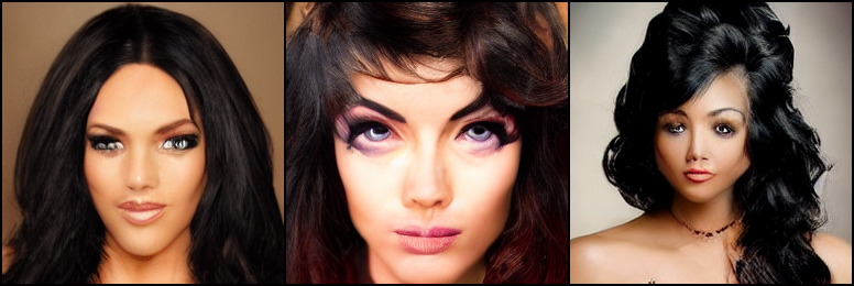
$\epsilon=1$

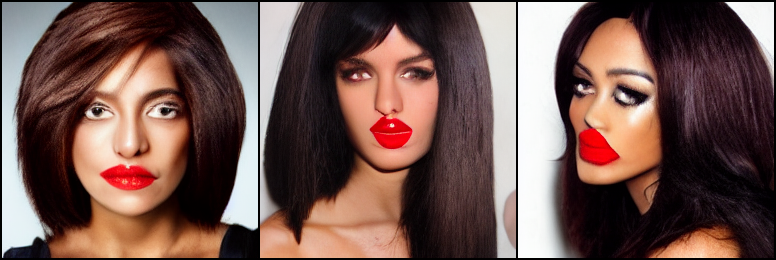
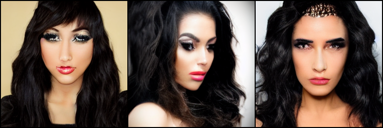
Figure 4: Text-to-image generation for CelebAHQ 256 by 256 with three sample prompt inputs. Privacy condition is set to $\epsilon=10,1$ and $\delta=10^{-5}$.

Class conditional generation. We build our model on the LDM model provided by Rombach et al. (2022) which is pretrained on Imagenet at a resolution of $256\times 256$. Following our experiments in Section 5.2, we fine-tune all of the SpatialTransformer blocks. While CelebAHQ does not provide class labels, each image is associated with 40 binary attributes. We choose the attribute “Male” to act as a binary class label for each image. Generated samples are available in Figure 5 along with FID values. Compared to DP-MEPF, based on the FID scores and perceptual image quality, DP-LDM is better suited for generating detailed, plausible samples from the high-resolution dataset at a wide range of privacy levels.

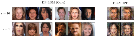
Figure 5: Synthetic $256\times 256$ CelebA samples generated at different levels of privacy. Samples for DP-MEPF are generated from code available in Harder et al. (2023). We computed FID between our generated samples and the real data and achieve FIDs of $19.0\pm 0.0$ at $\epsilon=10$, $20.5\pm 0.1$ at $\epsilon=5$, and $25.6\pm 0.1$ at $\epsilon=1$. DP-MEPF achieves an FID of $200.8$ at $\epsilon=10$ and $293.3$ at $\epsilon=1$.

6 Conclusion and Discussion

In Differentially Private Latent Diffusion Models (DP-LDM), we utilize DP-SGD to finetune only the attention modules (and embedders for conditioned generation) of the pretrained LDM at varying layers with privacy-sensitive data. We demonstrate that our method is capable of generating images for simple datasets like MNIST, more complex datasets like CIFAR-10 and CelebA, and high-dimensional datasets like CelebAHQ. We perform an in-depth analysis of ablation of DP-LDM to explore the strategy to reducing parameters for more applicable training of DP-SGD. Based on our promising results, we conclude that fine-tuning LDMs is an efficient and effective framework for DP generative learning. We hope our results can contribute to future research in DP data generation, considering the rapid advances in diffusion-based generative modelling.

7 Ethics and reproducibility

As investigated in (Carlini et al., 2023), diffusion models can memorize individual images from the training data and gives the same as generating samples. Aiming to bringing positive effects to society, our research is driven by the necessity of robust and scalabel data privacy. However, it is also important to approach the use of public data cautiously. As (Tramèr et al., 2022) pointed out, public data themselves may still be sensitive due to lack of curation practices. In addition, the public data usually achieve similar distribution as the private data, however, no proper public data is available currently as this might require heavy domain shift of the data themselves. We understand these potential issues but current DP machine learning research leads to minimal effects because of the inadequacy of the utility. From our perspective, auxiliary public data still emerges as the most promising option for attaining satisfactory utility, comparing to the potential harm it might inject. We hope our discussion will contribute to further research in differential privacy in machine learning using public data.

To guarantee the reproduciblity, our code is available at https://anonymous.4open.science/r/DP-LDM-4525 with detailed instructions. And all the hyperparameters are discussed in detail in Appendix Sec. B.

Appendix

Appendix A Additional Experiments

A.1 Scaling factor effect in pre-training the autoencoder

In Table  6, we provide FID results after pre-training the autoencoder with Imagenet dataset for different scaling factors $f$ and number of channels.

Table 6: FID scores (lower is better) for pre-trained autoencoders with different $f$ and number of channels.

	$\#$ channels
	128	64	32
$f=2$	27.6	36.4	46.8
$f=4$	32.9	51.0	83.5

A.2 Transferring from EMNIST to MNIST distribution

Here we compare DP-LDM to existing methods with the most common DP settings $\epsilon=1,10$ and $\delta=10^{-5}$ in Table  7.

Table 7: Downstream accuracies by CNN and WRN-40-4, evaluated on the generated MNIST data samples. We compare our results with existing work DPDM (Dockhorn et al., 2023), DP-Diffusion (Ghalebikesabi et al., 2023), PEARL (Liew et al., 2022b), DPGANr (Bie et al., 2022), and DP-HP (Vinaroz et al., 2022).

		DP-LDM (Ours)	DP-DM	DP-Diffusion	DP-HP	PEARL	DPGANr
$\epsilon=10$	CNN	$97.4\pm$ 0.1	98.1	-	-	78.8	95.0
	WRN	$97.5\pm$ 0.0	-	98.6	-	-	-
$\epsilon=1$	CNN	95.9$\pm$ 0.1	95.2	-	81.5	78.2	80.1
	# params	0.8M	1.75M	4.2M	-	-	-
	GPU Hours	10h	192h	-	-	-	-

A.2.1 Choose public dataset from SVHN, KMNIST and EMNIST for MNIST

We consider SVHN (street number digit but 3 channels), KMNIST (Japanese character in MNIST format 1 channel), and EMNIST (English letter in MNIST format 1 channel) as public dataset candidates. In general, if the two datasets are close to each other, then transfer learning from one to another is assumed to achieve better results within few iterations. To choose the best candidate, we compute the FID between each one with respect to MNIST and pick EMNIST as the public dataset in the end. We also did additional experiments using SVHN and KMNIST under the same privacy condition $\epsilon=10,\delta=10^{-5}$ in Table  8, which furthermore verifies our choice of EMNIST.

Table 8: FID scores for datasets with respect to MNIST. We also pretrained LDMs using SVHN and KMNIST then fine-tuned with MNIST, and list the best CNN accuracy here respectively.

Dataset pair	FID	Best CNN accuracy
(SVHN, MNIST)	231.6	94.3
(KMNIST, MNIST)	53.7	96.3
(EMNIST, MNIST)	27.5	97.4

A.2.2 Ablation experiments for MNIST

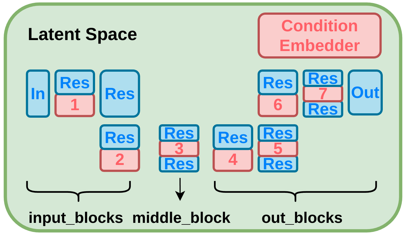
Figure 6: Unet Structure for MNIST.

There are 7 attention modules in the Unet structure for MNIST, 1-2 are in input_blocks, 3 is in middle_block, 4-7 are in out_blocks as illustrated in Fig. 6. Modules in blue are frozen during fine-tuning. Parameters of condition embedder is always trained. We consider fine tune only $i$-th to 7th attention modules to reduce more trainable parameters. Results for $\epsilon=10,\delta=10^{-5}$ are listed in Table  9. The best results is achieved when fine tune with 4-7 attention blocks, which means out_blocks are more important than others during training.

Table 9: CNN accuracy and number of trainable parameters for MNIST ablation experiments with varying number of fine-tuning layers. Privacy condition is set to $\epsilon=10,\delta=10^{-5}$.

	1-7(all)	2-7	3-7	4-7	5-7
CNN	97.3	97.3	90	97.4	97.3
# of trainable params	1.6M	1.5M	1.2M	0.8M	0.5M
out of 4.6M total params	(34.3%)	(32.4%)	(25.2%)	(18.0%)	(10.9%)

A.3 Transferring from Imagenet to CIFAR10 distribution

Here, we provide the results for ablation experiments to test the performance of DP-LDM when fine-tuning only certain attention modules inside the pre-trained model and keeping the rest of the parameters fixed. There are 16 attention modules in total as illustrated in Fig. 7. Table  10 shows the FID obtained for $\epsilon=1,5,10$ and $\delta=10^{-5}$ for the different number of attention modules fine-tuned. The results show that fixing up to the first half of the attention layers in the LDM has a positive effect in terms of the FID (the lower the better) in our model.

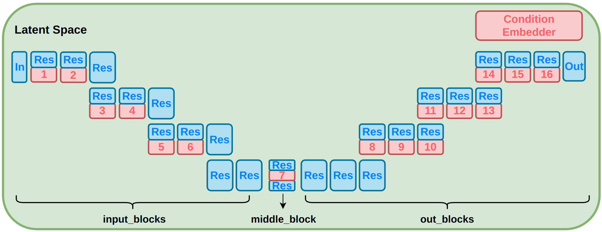
Figure 7: Unet Structure for CIFAR-10

Table 10: FID scores (lower is better) for synthetic CIFAR-10 data with varying the number of fine-tuning layers and privacy guarantees. Top row (1-16 layers): Fine-tuning all attention modules. Second row (5-16 layers): Keep first 4 attention modules fixed and fine-tuning from 5 to 16 attention modules. Third row (9-16 layers): Keep first 8 attention modules fixed and fine-tuning from 9 to 16 attention modules. Bottom row (13-16 layers): Keep first 12 attention modules fixed and fine-tuning from 13 to 16 attention modules.

DP-LDM	$\epsilon=10$	$\epsilon=5$	$\epsilon=1$
1-16 layers	25.8 $\pm$ 0.3	29.9 $\pm$ 0.2	33.0 $\pm$ 0.3
5 - 16 layers	15.7 $\pm$ 0.3	21.2 $\pm$ 0.2	28.9 $\pm$ 0.2
9 - 16 layers	8.4 $\pm$ 0.2	13.4 $\pm$ 0.4	22.9 $\pm$ 0.5
13 - 16 layers	12.3 $\pm$ 0.2	18.5 $\pm$ 0.2	25.2 $\pm$ 0.5

We also report the different hyper-parameter settings used in ablation experiments in table Table  11.

Table 11: DP-LDM hyper-parameter setting on CIFAR-10 for different ablation experiments.

		$\epsilon=10$	$\epsilon=5$	$\epsilon=1$
1-16 layers ($24.4$M parameters)	batch size	1000	2000	1000
	clipping norm	$10^{-5}$	$10^{-5}$	$10^{-3}$
	learning rate	$10^{-6}$	$10^{-6}$	$10^{-6}$
	epochs	30	30	10
5-16 layers ($20.8$M parameters)	batch size	5000	5000	2000
	clipping norm	$10^{-6}$	$10^{-5}$	$10^{-3}$
	learning rate	$10^{-6}$	$10^{-6}$	$10^{-5}$
	epochs	50	50	10
9-16 layers ($10.2$M parameters)	batch size	2000	2000	5000
	clipping norm	$10^{-6}$	$10^{-6}$	$10^{-2}$
	learning rate	$10^{-6}$	$10^{-6}$	$10^{-6}$
	epochs	30	30	10
13-16 layers ($4$M parameters)	batch size	2000	2000	2000
	clipping norm	$10^{-6}$	$10^{-6}$	$10^{-2}$
	learning rate	$10^{-6}$	$10^{-6}$	$10^{-6}$
	epochs	30	30	10

Table  12 shows the hyper-parameters used during training ResNet9 and WRN40-4 downstream classifiers on CIFAR10 synthetic samples.

Table 12: Hyperparameters for downstream classification ResNet9 and WRN40-4 trained on CIFAR10 synthetic data

	ResNet9	WRN40-4
learning rate	0.5	0.1
batch size	512	1000
epochs	10	10000
optimizer	SGD	SGD
label smoothing	0.1	0.0
weight decay	$5\cdot 10^{-4}$	$5\cdot 10^{-4}$
momentum	0.9	0.9

A.4 Transferring from Imagenet to CelebA32

We also apply our model in the task of generating $32\times 32$ CelebA images. The same pretrained autoencoder as our CIFAR-10 experiments in Section 5.1 is used, but since this experiment is for unconditional generation, we are unable to re-use the LDM. A new LDM is pretrained on Imagenet without class conditioning information, and then fine-tuned on CelebA images scaled and cropped to $32\times 32$ resolution. Our FID results for $\delta=10^{-6}$, $\epsilon=1,5,10$ are summarized in Table 13. We achieve similar results to DP-MEPF for $\epsilon=5$ and $\epsilon=10$. As with our results at $64\times 64$ resolution, our LDM model does not perform as well in higher privacy settings ($\epsilon=1$). Sample images are provided in Figure 8

Table 13: CelebA FID scores (lower is better) for images of resolution $32\times 32$ comparing with results from DPDM (Dockhorn et al., 2023), DP Sinkhorn (Cao et al., 2021), and DP-MEPF (Harder et al., 2023).

	$\epsilon=10$	$\epsilon=5$	$\epsilon=1$
DP-LDM (ours, average)	16.2 $\pm$ 0.2	16.8 $\pm$ 0.3	25.8 $\pm$ 0.9
DP-LDM (ours, best)	16.1	16.6	24.6
DP-MEPF $(\mathbf{\bm{\phi}}_{1})$	16.3	17.2	17.2
DP-GAN (pre-trained)	58.1	66.9	81.3
DPDM (no public data)	21.2	-	71.8
DP Sinkhorn (no public data)	189.5	-	-

Figure 8: Synthetic $32\times 32$ CelebA samples generated at different levels of privacy. Samples for DP-MERF and DP-Sinkhorn are taken from (Cao et al., 2021), DP-Diffusion samples are taken from (Dockhorn et al., 2023), and DP-MEPF samples are taken from (Harder et al., 2023).

Appendix B Hyperparameters

Here we provide an overview of the hyperparameters of the pretrained autoencoder in Table  14, hyperparameters of the pretrained diffusion models in Table  15. Note that $base\ learning\ rate$ is the one set in the yaml files. The real learning rate passed to the optimizer is $accumulate\_grad\_batches$ $\times$ $num\_gpus$ $\times$ $batch\ size$ $\times$ $base\ learning\ rate$.

Table 14: Hyperparameters for the pretrained autoencoders for different datasets.

	EMNIST	ImageNet	ImageNet	ImageNet
	(to MNIST)	(to CIFAR10)	(to CelebA 32)	(to CelebA 64)
Input size	32	32	32	64
Latent size	4	16	16	32
$f$	8	2	2	2
$z$-shape	$4\times 4\times 3$	$16\times 16\times 3$	$16\times 16\times 3$	$64\times 64\times 3$
Channels	128	128	128	192
Channel multiplier	[1,2,3,5]	[1,2]	[1,2]	[1,2]
Attention resolutions	[32,16,8]	[16, 8]	[16, 8]	[16,8]
num_res_blocks	2	2	2	2
Batch size	50	16	16	16
Base learning rate	$4.5\times 10^{-6}$	$4.5\times 10^{-6}$	$4.5\times 10^{-6}$	$1.0\times 10^{-6}$
Learning rate	$4.5\times 10^{-4}$	$1.4\times 10^{-4}$	$1.4\times 10^{-4}$	$1.4\times 10^{-4}$
Epochs	50	2	2	-
GPU(s)	1 NVIDIA V100	1 NVIDIA RTX A4000	1 NVIDIA RTX A4000	1 NVIDIA V100
Time	8 hours	1 day	1 day	1 day

Table 15: Hyperparameters for the pretrained diffusion models for different datasets.

	EMNIST	ImagNnet	ImageNet	ImageNet
	(to MNIST)	(to CIFAR10)	(to CelebA 32)	(to CelebA64)
input size	32	32	32	64
latent size	4	16	16	32
$f$	8	2	2	2
$z$-shape	$4\times 4\times 3$	$16\times 16\times 3$	$16\times 16\times 3$	$32\times 32\times 3$
channels	64	128	192	192
channel multiplier	[1,2]	[1,2,2,4]	[1,2,4]	[1,2,4]
attention resolutions	[1,2]	[1,2,4]	[1,2,4]	[1,2,4]
num_res_blocks	1	2	2	2
num_heads	2	8	-	8
num_head_channels	-	-	32	-
batch size	512	500	384	256
base learning rate	$5\times 10^{-6}$	$1\times 10^{-6}$	$5\times 10^{-7}$	$1\times 10^{-6}$
learning rate	$2.6\times 10^{-3}$	$5\times 10^{-4}$	$2\times 10^{-4}$	$2.6\times 10^{-4}$
epochs	120	30	13	40
# trainable parameters	4.6M	90.8M	162.3M	72.2M
GPU(s)	1 NVIDIA V100	1 NVIDIA RTX A4000	1 NVIDIA V100	1 NVIDIA V100
time	6 hours	7 days	30 hours	10 days
use_spatial_transformer	True	True	False	False
cond_stage_key	class_label	class_label	-	-
conditioning_key	crossattn	crossattn	-	-
num_classes	26	1000	-	-
embedding dimension	5	512	-	-
transformer depth	1	1	-	-

Table  16 shows the hyperparameters we used for fine-tuning on MNIST. Table  17 shows the hyperparameters we used for CelebA32. Table  18 shows the hyperparameters we used for CelebA64. Table  19 shows the hyperparameters we used for text-to-image CelebAHQ generation. Table  20 shows the hyperparmeters we used for class-conditioned CelebAHQ generation.

Table 16: Hyperparameters for fine-tuning diffusion models with DP constraints $\epsilon=10,1$ and $\delta=10^{-5}$ on MNIST. The “ablation” hyperparameter determines which attention modules are fine-tuned, where a value of $i$ means that the first $i-1$ attention modules are frozen and others are trained. Setting “ablation” to $-1$ (default) fine-tunes all attention modules.

	$\epsilon=10$	$\epsilon=1$
batch size	2000	2000
base learning rate	$5\times 10^{-7}$	$6\times 10^{-7}$
learning rate	$1\times 10^{-3}$	$1.2\times 10^{-3}$
epochs	200	200
clipping norm	0.01	0.001
noise scale	1.47	9.78
ablation	4	-1
num of params	0.8M	1.6M
use_spatial_transformer	True	True
cond_stage_key	class_label	class_label
conditioning_key	crossattn	crossattn
num_classes	26	26
embedding dimension	13	13
transformer depth	1	1
train_condition_only	True	True
attention_flag	spatial	spatial
# condition params	338	338

Table 17: Hyperparameters for fine-tuning diffusion models with DP constraints $\epsilon=10,5,1$ and $\delta=10^{-6}$ on CelebA32.

	$\epsilon=10$	$\epsilon=5$	$\epsilon=1$
batch size	8192	8192	2048
base learning rate	$5\times 10^{-7}$	$5\times 10^{-7}$	$5\times 10^{-7}$
learning rate	$4\times 10^{-3}$	$4\times 10^{-3}$	$1\times 10^{-3}$
epochs	20	20	20
clipping norm	$5.0\times 10^{-4}$	$5.0\times 10^{-4}$	$5.0\times 10^{-4}$
ablation	-1	-1	-1
use_spatial_transformer	False	False	False
cond_stage_key	-	-	-
conditioning_key	-	-	-
num_classes	-	-	-
embedding dimension	-	-	-
transformer depth	-	-	-
train_attention_only	True	True	True

Table 18: Hyperparameters for fine-tuning diffusion models with DP constraints $\epsilon=10,5,1$ and $\delta=10^{-6}$ on CelebA64.

	$\epsilon=10$	$\epsilon=5$	$\epsilon=1$
batch size	8192	8192	8192
base learning rate	$1\times 10^{-7}$	$1\times 10^{-7}$	$1\times 10^{-7}$
learning rate	$8.2\times 10^{-4}$	$8.2\times 10^{-4}$	$8.2\times 10^{-4}$
epochs	70	70	70
clipping norm	$5.0\times 10^{-4}$	$5.0\times 10^{-4}$	$5.0\times 10^{-4}$
ablation	-1	-1	-1
use_spatial_transformer	False	False	False
cond_stage_key	-	-	-
conditioning_key	-	-	-
num_classes	-	-	-
embedding dimension	-	-	-
transformer depth	-	-	-
train_attention_only	True	True	True

Table 19: Hyperparameters for fine-tuning diffusion models with DP constraints $\epsilon=10,1$ and $\delta=10^{-5}$ on text-conditioned CelebAHQ.

	$\epsilon=10$	$\epsilon=1$
batch size	256	256
base learning rate	$1\times 10^{-7}$	$1\times 10^{-7}$
learning rate	$2.6\times 10^{-5}$	$2.6\times 10^{-5}$
epochs	10	10
clipping norm	0.01	0.01
noise scale	0.55	1.46
ablation	-1	-1
num of params	280M	280M
use_spatial_transformer	True	True
cond_stage_key	caption	caption
context_dim	1280	1280
conditioning_key	crossattn	crossattn
transformer depth	1	1

Table 20: Hyperparameters for fine-tuning diffusion models with DP constraints $\epsilon=10,5,1$ and $\delta=10^{-5}$ on class-conditional CelebAHQ.

	$\epsilon=10$	$\epsilon=5$	$\epsilon=1$
batch size	2048	2048	2048
base learning rate	$1\times 10^{-7}$	$1\times 10^{-7}$	$1\times 10^{-7}$
learning rate	$2.0\times 10^{-4}$	$2.0\times 10^{-4}$	$2.0\times 10^{-4}$
epochs	50	50	50
clipping norm	$5.0\times 10^{-4}$	$5.0\times 10^{-4}$	$5.0\times 10^{-4}$
ablation	-1	-1	-1
use_spatial_transformer	True	True	True
cond_stage_key	class_label	class_label	class_label
context_dim	512	512	512
conditioning_key	crossattn	crossattn	crossattn
transformer depth	1	1	1

Appendix C Additional Samples

References

- Abadi et al. (2016) Martin Abadi, Andy Chu, Ian J. Goodfellow, H. Brendan McMahan, Ilya Mironov, Kunal Talwar, and Li Zhang. Deep learning with differential privacy. In Proceedings of the 2016 ACM SIGSAC Conference on Computer and Communications Security, CCS ’16, pp. 308–318, New York, NY, USA, 2016. Association for Computing Machinery. ISBN 9781450341394. doi: 10.1145/2976749.2978318.
- Acs et al. (2018) Gergely Acs, Luca Melis, Claude Castelluccia, and Emiliano De Cristofaro. Differentially private mixture of generative neural networks. IEEE Transactions on Knowledge and Data Engineering, 31(6):1109–1121, 2018.
- Bie et al. (2022) Alex Bie, Gautam Kamath, and Guojun Zhang. Private GANs, revisited. In NeurIPS 2022 Workshop on Synthetic Data for Empowering ML Research, 2022.
- Bu et al. (2022) Zhiqi Bu, Jialin Mao, and Shiyun Xu. Scalable and efficient training of large convolutional neural networks with differential privacy, 2022.
- Cao et al. (2021) Tianshi Cao, Alex Bie, Arash Vahdat, Sanja Fidler, and Karsten Kreis. Don’t generate me: Training differentially private generative models with sinkhorn divergence. In Neural Information Processing Systems (NeurIPS), 2021.
- Carlini et al. (2023) Nicholas Carlini, Jamie Hayes, Milad Nasr, Matthew Jagielski, Vikash Sehwag, Florian Tramer, Borja Balle, Daphne Ippolito, and Eric Wallace. Extracting training data from diffusion models. arXiv preprint arXiv:2301.13188, 2023.
- Chen et al. (2020) Dingfan Chen, Tribhuvanesh Orekondy, and Mario Fritz. Gs-wgan: A gradient-sanitized approach for learning differentially private generators. In Advances in Neural Information Processing Systems 33, 2020.
- Chen et al. (2015) Rui Chen, Qian Xiao, Yu Zhang, and Jianliang Xu. Differentially private high-dimensional data publication via sampling-based inference. In Proceedings of the 21th ACM SIGKDD International Conference on Knowledge Discovery and Data Mining, pp. 129–138, 2015.
- Clanuwat et al. (2018) Tarin Clanuwat, Mikel Bober-Irizar, Asanobu Kitamoto, Alex Lamb, Kazuaki Yamamoto, and David Ha. Deep learning for classical japanese literature. arXiv preprint arXiv:1812.01718, 2018.
- Cohen et al. (2017) Gregory Cohen, Saeed Afshar, Jonathan Tapson, and Andre Van Schaik. Emnist: Extending mnist to handwritten letters. In 2017 international joint conference on neural networks (IJCNN), pp. 2921–2926. IEEE, 2017.
- De et al. (2022) Soham De, Leonard Berrada, Jamie Hayes, Samuel L. Smith, and Borja Balle. Unlocking high-accuracy differentially private image classification through scale, 2022.
- Deng et al. (2009) Jia Deng, Wei Dong, Richard Socher, Li-Jia Li, Kai Li, and Li Fei-Fei. Imagenet: A large-scale hierarchical image database. In 2009 IEEE conference on computer vision and pattern recognition, pp. 248–255. Ieee, 2009.
- Devlin et al. (2018) Jacob Devlin, Ming-Wei Chang, Kenton Lee, and Kristina Toutanova. Bert: Pre-training of deep bidirectional transformers for language understanding. arXiv preprint arXiv:1810.04805, 2018.
- Dockhorn et al. (2023) Tim Dockhorn, Tianshi Cao, Arash Vahdat, and Karsten Kreis. Differentially private diffusion models, 2023. URL https://openreview.net/forum?id=pX21pH4CsNB.
- Dwork et al. (2006) Cynthia Dwork, Krishnaram Kenthapadi, Frank McSherry, Ilya Mironov, and Moni Naor. Our data, ourselves: Privacy via distributed noise generation. In Advances in Cryptology - EUROCRYPT 2006, 25th Annual International Conference on the Theory and Applications of Cryptographic Techniques, volume 4004 of Lecture Notes in Computer Science, pp. 486–503. Springer, 2006. doi: 10.1007/11761679˙29.
- Frigerio et al. (2019) Lorenzo Frigerio, Anderson Santana de Oliveira, Laurent Gomez, and Patrick Duverger. Differentially private generative adversarial networks for time series, continuous, and discrete open data. In ICT Systems Security and Privacy Protection - 34th IFIP TC 11 International Conference, SEC 2019, Lisbon, Portugal, June 25-27, 2019, Proceedings, pp. 151–164, 2019. doi: 10.1007/978-3-030-22312-0“˙11.
- Ghalebikesabi et al. (2023) Sahra Ghalebikesabi, Leonard Berrada, Sven Gowal, Ira Ktena, Robert Stanforth, Jamie Hayes, Soham De, Samuel L. Smith, Olivia Wiles, and Borja Balle. Differentially private diffusion models generate useful synthetic images, 2023.
- Goodfellow et al. (2014) I. J. Goodfellow, J. Pouget-Abadie, M. Mirza, B. Xu, D. Warde-Farley, S. Ozair, A. Courville, and Y. Bengio. Generative adversarial networks. In Advances in Neural Information Processing Systems, 2014.
- Harder et al. (2021) Frederik Harder, Kamil Adamczewski, and Mijung Park. DP-MERF: Differentially private mean embeddings with random features for practical privacy-preserving data generation. In AISTATS, volume 130 of Proceedings of Machine Learning Research, pp. 1819–1827. PMLR, 2021.
- Harder et al. (2023) Frederik Harder, Milad Jalali, Danica J. Sutherland, and Mijung Park. Pre-trained perceptual features improve differentially private image generation. Transactions on Machine Learning Research, 2023. ISSN 2835-8856. URL https://openreview.net/forum?id=R6W7zkMz0P.
- Hardt et al. (2012) Moritz Hardt, Katrina Ligett, and Frank Mcsherry. A simple and practical algorithm for differentially private data release. In Advances in Neural Information Processing Systems 25, pp. 2339–2347. Curran Associates, Inc., 2012.
- Hertz et al. (2022) Amir Hertz, Ron Mokady, Jay Tenenbaum, Kfir Aberman, Yael Pritch, and Daniel Cohen-Or. Prompt-to-prompt image editing with cross attention control, 2022.
- Heusel et al. (2017) Martin Heusel, Hubert Ramsauer, Thomas Unterthiner, Bernhard Nessler, and Sepp Hochreiter. Gans trained by a two time-scale update rule converge to a local nash equilibrium. Advances in neural information processing systems, 30, 2017.
- Ho et al. (2020) Jonathan Ho, Ajay Jain, and Pieter Abbeel. Denoising diffusion probabilistic models. In H. Larochelle, M. Ranzato, R. Hadsell, M.F. Balcan, and H. Lin (eds.), Advances in Neural Information Processing Systems, volume 33, pp. 6840–6851. Curran Associates, Inc., 2020. URL https://proceedings.neurips.cc/paper_files/paper/2020/file/4c5bcfec8584af0d967f1ab10179ca4b-Paper.pdf.
- Hu et al. (2021) Edward J. Hu, Yelong Shen, Phillip Wallis, Zeyuan Allen-Zhu, Yuanzhi Li, Shean Wang, Lu Wang, and Weizhu Chen. Lora: Low-rank adaptation of large language models, 2021.
- Jiang et al. (2022) Dihong Jiang, Guojun Zhang, Mahdi Karami, Xi Chen, Yunfeng Shao, and Yaoliang Yu. Dp2-vae: Differentially private pre-trained variational autoencoders. arXiv preprint arXiv:2208.03409, 2022.
- Krizhevsky et al. (2009) Alex Krizhevsky, Geoffrey Hinton, et al. Learning multiple layers of features from tiny images. Technical report, University of Toronto, Toronto, ON, Canada, 2009.
- LeCun & Cortes (2010) Yann LeCun and Corinna Cortes. MNIST handwritten digit database. http://yann.lecun.com/exdb/mnist/, 2010. URL http://yann.lecun.com/exdb/mnist/.
- Liew et al. (2022a) Seng Pei Liew, Tsubasa Takahashi, and Michihiko Ueno. PEARL: Data synthesis via private embeddings and adversarial reconstruction learning. In International Conference on Learning Representations, 2022a.
- Liew et al. (2022b) Seng Pei Liew, Tsubasa Takahashi, and Michihiko Ueno. PEARL: Data synthesis via private embeddings and adversarial reconstruction learning. In International Conference on Learning Representations, 2022b.
- Lin et al. (2023) Zinan Lin, Sivakanth Gopi, Janardhan Kulkarni, Harsha Nori, and Sergey Yekhanin. Differentially private synthetic data via foundation model apis 1: Images, 2023.
- Liu et al. (2015) Ziwei Liu, Ping Luo, Xiaogang Wang, and Xiaoou Tang. Deep learning face attributes in the wild. In Proceedings of International Conference on Computer Vision (ICCV), December 2015.
- Mohammed et al. (2011) Noman Mohammed, Rui Chen, Benjamin C.M. Fung, and Philip S. Yu. Differentially private data release for data mining. In Proceedings of the 17th ACM SIGKDD International Conference on Knowledge Discovery and Data Mining, KDD ’11, pp. 493–501, New York, NY, USA, 2011. ACM. ISBN 978-1-4503-0813-7. doi: 10.1145/2020408.2020487.
- Netzer et al. (2011) Yuval Netzer, Tao Wang, Adam Coates, Alessandro Bissacco, Bo Wu, and Andrew Y Ng. Reading digits in natural images with unsupervised feature learning. 2011.
- Papernot et al. (2017) Nicolas Papernot, Martín Abadi, Úlfar Erlingsson, Ian J. Goodfellow, and Kunal Talwar. Semi-supervised knowledge transfer for deep learning from private training data. In Proceedings of the International Conference on Learning Representations (ICLR), 2017.
- Park et al. (2023) Dong Huk Park, Grace Luo, Clayton Toste, Samaneh Azadi, Xihui Liu, Maka Karalashvili, Anna Rohrbach, and Trevor Darrell. Shape-guided diffusion with inside-outside attention, 2023.
- Paszke et al. (2019) Adam Paszke, Sam Gross, Francisco Massa, Adam Lerer, James Bradbury, Gregory Chanan, Trevor Killeen, Zeming Lin, Natalia Gimelshein, Luca Antiga, et al. Pytorch: An imperative style, high-performance deep learning library. Advances in neural information processing systems, 32, 2019.
- Pfitzner & Arnrich (2022) Bjarne Pfitzner and Bert Arnrich. Dpd-fvae: Synthetic data generation using federated variational autoencoders with differentially-private decoder. arXiv preprint arXiv:2211.11591, 2022.
- Ponomareva et al. (2023) Natalia Ponomareva, Sergei Vassilvitskii, Zheng Xu, Brendan McMahan, Alexey Kurakin, and Chiyaun Zhang. How to dp-fy ml: A practical tutorial to machine learning with differential privacy. In Proceedings of the 29th ACM SIGKDD Conference on Knowledge Discovery and Data Mining, KDD ’23, pp. 5823–5824, New York, NY, USA, 2023. Association for Computing Machinery. ISBN 9798400701030. doi: 10.1145/3580305.3599561. URL https://doi.org/10.1145/3580305.3599561.
- Qardaji et al. (2014) Wahbeh Qardaji, Weining Yang, and Ninghui Li. Priview: practical differentially private release of marginal contingency tables. In Proceedings of the 2014 ACM SIGMOD international conference on Management of data, pp. 1435–1446, 2014.
- Rombach et al. (2022) Robin Rombach, Andreas Blattmann, Dominik Lorenz, Patrick Esser, and Björn Ommer. High-resolution image synthesis with latent diffusion models. In Proceedings of the IEEE/CVF Conference on Computer Vision and Pattern Recognition (CVPR), pp. 10684–10695, June 2022.
- Schuhmann et al. (2021) Christoph Schuhmann, Richard Vencu, Romain Beaumont, Robert Kaczmarczyk, Clayton Mullis, Aarush Katta, Theo Coombes, Jenia Jitsev, and Aran Komatsuzaki. Laion-400m: Open dataset of clip-filtered 400 million image-text pairs. arXiv preprint arXiv:2111.02114, 2021.
- Snoke & Slavković (2018) Joshua Snoke and Aleksandra Slavković. pmse mechanism: differentially private synthetic data with maximal distributional similarity. In International Conference on Privacy in Statistical Databases, pp. 138–159. Springer, 2018.
- Song et al. (2021) Yang Song, Jascha Sohl-Dickstein, Diederik P Kingma, Abhishek Kumar, Stefano Ermon, and Ben Poole. Score-based generative modeling through stochastic differential equations. International Conference on Learning Representations, 2021.
- Torkzadehmahani et al. (2019) Reihaneh Torkzadehmahani, Peter Kairouz, and Benedict Paten. Dp-cgan: Differentially private synthetic data and label generation. In The IEEE Conference on Computer Vision and Pattern Recognition (CVPR) Workshops, June 2019.
- Tramèr et al. (2022) Florian Tramèr, Gautam Kamath, and Nicholas Carlini. Considerations for differentially private learning with large-scale public pretraining. arXiv preprint arXiv:2212.06470, 2022.
- Vinaroz et al. (2022) Margarita Vinaroz, Mohammad-Amin Charusaie, Frederik Harder, Kamil Adamczewski, and Mi Jung Park. Hermite polynomial features for private data generation. In ICML, volume 162 of Proceedings of Machine Learning Research, pp. 22300–22324. PMLR, 2022.
- Xia et al. (2021) Weihao Xia, Yujiu Yang, Jing-Hao Xue, and Baoyuan Wu. Tedigan: Text-guided diverse face image generation and manipulation. In Proceedings of the IEEE/CVF conference on computer vision and pattern recognition, pp. 2256–2265, 2021.
- Xiao et al. (2010) Yonghui Xiao, Li Xiong, and Chun Yuan. Differentially private data release through multidimensional partitioning. In Secure Data Management, pp. 150–168, Berlin, Heidelberg, 2010. Springer Berlin Heidelberg. ISBN 978-3-642-15546-8.
- Xie et al. (2018) Liyang Xie, Kaixiang Lin, Shu Wang, Fei Wang, and Jiayu Zhou. Differentially private generative adversarial network. arXiv preprint arXiv:1802.06739, 2018.
- Yang et al. (2023) Yilin Yang, Kamil Adamczewski, Danica J. Sutherland, Xiaoxiao Li, and Mijung Park. Differentially private neural tangent kernels for privacy-preserving data generation, 2023.
- Yoon et al. (2019) Jinsung Yoon, James Jordon, and Mihaela van der Schaar. PATE-GAN: Generating synthetic data with differential privacy guarantees. In International Conference on Learning Representations, 2019.
- You & Zhao (2023) Fuming You and Zhou Zhao. Transferring pretrained diffusion probabilistic models, 2023. URL https://openreview.net/forum?id=8u9eXwu5GAb.
- Yousefpour et al. (2021) Ashkan Yousefpour, Igor Shilov, Alexandre Sablayrolles, Davide Testuggine, Karthik Prasad, Mani Malek, John Nguyen, Sayan Ghosh, Akash Bharadwaj, Jessica Zhao, Graham Cormode, and Ilya Mironov. Opacus: User-friendly differential privacy library in PyTorch. arXiv preprint arXiv:2109.12298, 2021.
- Yu et al. (2022) Da Yu, Saurabh Naik, Arturs Backurs, Sivakanth Gopi, Huseyin A Inan, Gautam Kamath, Janardhan Kulkarni, Yin Tat Lee, Andre Manoel, Lukas Wutschitz, Sergey Yekhanin, and Huishuai Zhang. Differentially private fine-tuning of language models. In International Conference on Learning Representations, 2022. URL https://openreview.net/forum?id=Q42f0dfjECO.
- Zhang et al. (2017) Jun Zhang, Graham Cormode, Cecilia M Procopiuc, Divesh Srivastava, and Xiaokui Xiao. Privbayes: Private data release via bayesian networks. ACM Transactions on Database Systems (TODS), 42(4):1–41, 2017.
- Zhang et al. (2023) Lvmin Zhang, Anyi Rao, and Maneesh Agrawala. Adding conditional control to text-to-image diffusion models, 2023.
- Zhang et al. (2021) Zhikun Zhang, Tianhao Wang, Ninghui Li, Jean Honorio, Michael Backes, Shibo He, Jiming Chen, and Yang Zhang. Privsyn: Differentially private data synthesis. In 30th USENIX Security Symposium (USENIX Security 21), 2021.
- Zhu et al. (2017) T. Zhu, G. Li, W. Zhou, and P. S. Yu. Differentially private data publishing and analysis: A survey. IEEE Transactions on Knowledge and Data Engineering, 29(8):1619–1638, August 2017. ISSN 1041-4347. doi: 10.1109/TKDE.2017.2697856.