Bayesian Analysis for Over-parameterized Linear Model
without Sparsity

Abstract.

In high-dimensional Bayesian statistics, several methods have been developed, including many prior distributions that lead to the sparsity of estimated parameters. However, such priors have limitations in handling the spectral eigenvector structure of data, and as a result, they are ill-suited for analyzing over-parameterized models (high-dimensional linear models that do not assume sparsity) that have been developed in recent years. This paper introduces a Bayesian approach that uses a prior dependent on the eigenvectors of data covariance matrices, but does not induce the sparsity of parameters. We also provide contraction rates of derived posterior distributions and develop a truncated Gaussian approximation of the posterior distribution. The former demonstrates the efficiency of posterior estimation, while the latter enables quantification of parameter uncertainty using a Bernstein-von Mises-type approach. These results indicate that any Bayesian method that can handle the spectrum of data and estimate non-sparse high dimensions would be possible.

1. Introduction

1.1. Overview

We consider an over-parameterized linear regression problem. Suppose that we observe $n$ independent pairs of responses and $p$-dimensional random covariates $(y_{1},\bm{x}_{1}),...,(y_{n},\bm{x}_{n})\in\mathbb{R}\times\mathbb{R}^{p}$ that are identically generated from the following regression model for $i=1,\ldots,n$:

$$y_{i}=\bm{x}_{i}^{\top}\bm{\theta}^{*}+\varepsilon_{i},$$ (1)

where $\varepsilon_{i}$ is an independent noise from $N(0,(\sigma^{*})^{2})$ and $\bm{\theta}^{*}\in\mathbb{R}^{p}$ and $\sigma^{*}$ are the true parameters. Here, the dimension $p$ is allowed to be much larger than the sample size $n$, i.e. $p\gg n$, and we assume that almost every coordinate of the covariate $\bm{x}_{i}$ is relevant to the response $y_{i}$, which implies the non-sparsity of $\bm{\theta}^{*}$. This paper studies a Bayesian method for the model (1) by developing a prior distribution on parameters $\bm{\theta}$, then investigates its associated posterior distribution under certain assumptions on the covariates.

In the realm of over-parametrized Bayesian statistics, a plethora of prior distributions leveraging sparsity have been developed to effectively handle $p$ parameters with large $p$. Specifically, starting with double exponential prior for Bayesian lasso [40], many prior distributions for the linear regression problem [e.g., 17, 41] have been incorporated into the extraction of information from an excess number of covariates. Notably, these methodologies are highly adept at deriving insights from a vast amount of data and selectively determining whether components of parameter vectors should be estimated either as zero or non-zero. While these approaches have demonstrated interpretability and theoretical underpinnings [18, 39], they necessitate the stringent assumption that most coordinates of the regression parameters are zero (or close to zero).

On the other hand, within a frequentist framework, several studies have focused on a non-sparse high-dimensional model, commonly known as an over-parameterized model, which is motivated by the success of large-scale models such as deep learning [29]. These methods mainly use spectral properties of data, i.e., eigenvalues and eigenvectors of the covariance matrix of the covariates. [20] and [26] studied ridge and ridgeless estimators of a linear regression model and derived a precious estimation error in a high-dimensional limit such that $p\to\infty$. [10] and [45] investigated the estimators for linear regression, then showed that the risks of the estimators are independent of dimension $p$ but described by an effective rank of a covariance matrix of covariates. These results have led to a great deal of subsequent research on high-dimensional statistics that do not rely on sparsity, as listed in Section 1.2. One limitation of the Bayesian methods in this context is that they cannot be applied to the over-parameterized model because high-dimensional Bayesian methods that rely on sparsity do not allow such spectral control. Therefore, a new prior distribution must be designed to handle over-parameterized models.

In this work, we develop a prior distribution for an over-parameterized linear regression and examine the theoretical features of its corresponding posterior distribution. The prior is $p$-dimensional Gaussian with a given covariance matrix using eigenvalues and eigenvectors estimated from the data in an empirical Bayesian manner, and the number of eigenvalues is selected by a hierarchical Bayesian approach. To study the posterior distribution, we introduce an assumption on a spectral structure on covariance matrices of covariates, as same to that of [10]. As a main contribution, we show the contraction of the posterior distribution toward the true parameter and also show its contraction rate. These results imply that a prediction risk of a mean of the posterior converges to zero. Another contribution is to develop a useful approximator of the posterior distribution, which is an over-parameterized version of the Bernstein-von Mises theorem [23, 24, 12]. This approximation is instantly obtained without running onerous Bayesian computations such as Markov chain Monte-Carlo, that are slow to converge in high dimensional spaces. The results are also broadly applicable in practice, for example, in constructing credible intervals for parameters and forecasts. Furthermore, our framework relaxes the assumption on the distribution of covariates, imposed by previous over-parameterized regression theories.

From a technical perspective, this study makes two contributions. The first is the analysis of a prior distribution with a singular covariance that corresponds to the intrinsic low-dimensionality of the data distribution. Since the data in our setting have low-dimensionality through its eigenvalue decay, we design the prior on a suitable low-dimensional sublinear space through an empirical covariance matrix with a truncation of eigenvalues. This design allows the complexity of the parameters determined to fit the intrinsic low-dimensionality of the covariates. The second is the derivation of our proof that allows for a simpler treatment of the distribution of covariates. That is, we can easily handle the heavy-tail property of covariates in our proof for the benign overfitting. By the proof, we apply the recent development of dimension-free bounds with heavy-tail distributions [37, 56] to our analysis.

1.2. Related Work

There is abundant literature on Bayesian methods for linear regression models. For high-dimensional problems, prior distributions, taking care of the sparsity structure, were developed such as Laplace [40], horseshoe prior [17], the spike and slab prior [41], the normal-gamma prior [7], the double-Pareto prior [2], the Dirichlet–Laplace (DL) prior [13], the horseshoe+ prior [6] and the triple gamma prior [14].

Regarding the asymptotic behavior of the posterior distribution, [22, 23, 24] examine the approximation of the posterior distribution by a Gaussian distribution in a variety of situations, including a high dimensional setting (not over-parameterized setting). [21] organized the conditions for posterior contraction and made a significant contribution to Bayes’ asymptotic theory. [19, 11] proved posterior concentration and variable selection properties for certain point-mass priors. [18, 35, 9, 11] achieved posterior concentration and variable selection in high dimensional linear models. [1] showed posterior consistency with several shrinkage priors. [49] showed that the posterior concentration with the horseshoe prior. [13] showed the result using the DL prior. [8, 43] considered a general class of continuous shrinkage priors. [39] considers variable selection with unknown covariance matrix and established posterior consistency result. [57, 54] studied efficiency and the Gaussian approximation of a coordinate of the high dimensional parameters. [5] provided a detailed review of these references.

There has been a rapidly growing body of theoretical work on the frequentist analysis of over-parameterized models, that is, on benign overfitting. A theory closely related to our work is [10], which showed that excess risk converges to zero in an over-parameterized linear model. The phenomenon has been studied in other situations such as regularized regressions [45, 28, 52, 33, 16], logistic regressions [15, 36], kernel regressions [31, 32], and regressions for dependent data [38, 48].

1.3. Paper Organization

The remainder of the paper is structured as follows. Section 2 describes the prior design. In Section 3, we provide our theoretical results about posterior distribution. Section 4 explains a sketch of the proof. In Section 5, we confirm our theoretical results through numerical experiments. Section 6 presents a conclusion and discusses our contributions. Appendices A and B contain proofs of the theorems.

1.4. Notation

For $n\in\mathbb{N}$ and any vector $\bm{v}$, $\|\bm{v}\|_{n}$ denotes an $\ell_{n}$-norm of $\bm{v}$. For any vector $\bm{v}$ and a matrix of the same dimension $A$, we define $\|\bm{v}\|_{A}=\sqrt{\bm{v}^{\top}A\bm{v}}$. $a_{n}\gtrsim b_{n}$ denotes that there exists a constant $c>0$ such that $a_{n}\geq cb_{n}$ for all $n\geq\overline{n}$ with some finite $\overline{n}\in\mathbb{N}$; $a_{n}\lesssim b_{n}$ denotes its opposite. For any matrix $A$, let $A^{-1}$ be the inverse matrix of $A$, and $A^{\dagger}$ be the Moore–Penrose inverse matrix. For a pseudo-metric space $(\Omega,d)$ and a positive value $\delta$, $\mathcal{N}(\delta,\Omega,d)$ denotes the covering number, that is, the minimum number of balls that cover $\Omega$, with the radius $\delta$ in terms of $d$, and $\mathcal{M}(\delta,\Omega,d)$ denotes the packing number, that is, the maximum number of balls of radius $\delta/2$ in terms of $d$, whose centers are in $\Omega$, such that no two balls intersect. The total variation distance between $\Pi_{1}$ and $\Pi_{2}$ are given by $\|\Pi_{1}-\Pi_{2}\|_{\mathrm{TV}}$. The Kullback-Leibler divergence and the Kullback-Leibler variation between $p$ and $q$ are defined as $K(p,q)=\int p\log(p/q)$ and $V(p,q)=\int p\{\log(p/q)-K(p,q)\}^{2}$, respectively. $a_{n}=o(b_{n})$ means $a_{n}/b_{n}\to 0$ as $n\to\infty$, $a_{n}=\omega(b_{n})$ does $a_{n}/b_{n}\to\infty$ as $n\to\infty$.

2. Prior Design

We consider a linear regression model (1), from the independent identically distributed samples $\mathcal{D}=\{y_{i},\bm{x}_{i}\}_{i=1}^{n}$, and perform prediction in a Bayesian manner. To this end, we construct the prior distributions in this section. Suppose $\bm{x}$ is a random vector distributed to non-atomic distribution.

2.1. Preparation

To begin with, we split the dataset $\mathcal{D}$ to $\mathcal{D}_{1}$ and $\mathcal{D}_{2}$. The split ratio can be any, as long as it does not depend on $n$. Without loss of generality, we assume that $n$ is even and define $\mathcal{D}_{1}=\{y_{i},\bm{x}_{i}\}_{i=1}^{n/2}$ and $\mathcal{D}_{2}=\{y_{i},\bm{x}_{i}\}_{i=n/2+1}^{n}$. Note that $\mathcal{D}_{1}$ is used to construct the prior distribution and $\mathcal{D}_{2}$ serves as the likelihood. Next, we consider a covariance matrix $\Sigma:=E[\bm{x}\bm{x}^{\top}]$ and its empirical analogue $\widehat{\Sigma}:=\frac{2}{n}\sum_{i=1}^{n/2}\bm{x}_{i}\bm{x}^{\top}_{i}$ by $\mathcal{D}_{1}$, and also define their spectral decompositions:

$$\Sigma=\sum_{j=1}^{p}\lambda_{j}\bm{v}_{j}\bm{v}_{j}^{\top},\mbox{~{}and~{}}\ \widehat{\Sigma}=\sum_{j=1}^{p}\widehat{\lambda}_{j}\widehat{\bm{v}}_{j}\widehat{\bm{v}}_{j}^{\top},$$

where $\{\lambda_{j}\}$ are eigenvalues sorted in descending order as $\lambda_{1}\geq\lambda_{2}\geq\ldots\geq\lambda_{p}$, $\{\bm{v}_{j}\}$ are corresponding eigenvectors, $\widehat{\Sigma}$, $\{\widehat{\lambda}_{j}\}$ and $\{\widehat{\bm{v}}_{j}\}$ respectively denote empirical covariance, its eigenvalues, and eigenvectors for dataset $\mathcal{D}_{1}$. Here, $\widehat{\lambda}_{j}=0$ for $j=n/2+1,\ldots,p$ and, for $j=n/2+1,\ldots,p$, $\widehat{\lambda}_{j}$ and $\widehat{v}_{j}$ converge to the $\lambda_{j}$ and $v_{j}$, respectively, depending on the complexity of $\Sigma$ and distribution of $\bm{x}$ [e.g., 27].

We further define a low-rank approximation of $\Sigma$ and $\widehat{\Sigma}$ with a truncation level $k^{*}\in\{1,2,\ldots,p\}$. That is, we define

$$\Sigma=\Sigma_{1}+\Sigma_{2}:=\sum_{j=1}^{k^{*}}\lambda_{j}\bm{v}_{j}\bm{v}_{j}^{\top}+\sum_{j=k^{*}+1}^{p}\lambda_{j}\bm{v}_{j}\bm{v}_{j}^{\top},\mbox{~{}and~{} }\ \widehat{\Sigma}=\widehat{\Sigma}_{1}+\widehat{\Sigma}_{2}:=\sum_{j=1}^{k^{*}}\widehat{\lambda}_{j}\widehat{\bm{v}}_{j}\widehat{\bm{v}}_{j}^{\top}+\sum_{j=k^{*}+1}^{p}\widehat{\lambda}_{j}\widehat{\bm{v}}_{j}\widehat{\bm{v}}_{j}^{\top}.$$

$\Sigma_{1}$ and $\widehat{\Sigma}_{1}$ respectively represent the approximations of $\Sigma$ and $\widehat{\Sigma}$, and $\Sigma_{2}$ and $\widehat{\Sigma}_{2}$ are the remaining parts. There are many studies that consider the low-rank nature of matrices in the Bayesian context [e.g., 3, 47].

We allow $\bm{\theta}$ and $\sigma$ to be independent in the prior.

2.2. Prior for Regression Parameters

We develop the following truncated Gaussian prior distribution:

$$\Pi_{\bm{\theta}}(\bm{\theta}\mid\widehat{\Sigma}_{1}) =\frac{\exp\big{(}-\bm{\theta}^{\top}\widehat{\Sigma}_{1}^{\dagger}\bm{\theta}\big{)}\textbf{1}\{\|\bm{\theta}\|_{2}\leq R\}}{\int_{\mathbb{R}^{p}}\exp\big{(}-\bm{\theta}^{\prime\top}\widehat{\Sigma}_{1}^{\dagger}\bm{\theta}^{\prime}\big{)}\textbf{1}\{\|\bm{\theta}^{\prime}\|_{2}\leq R\}d\bm{\theta}^{\prime}},$$

where $R$ denotes the radius of the support of distribution. We suppose $R$ is a sufficiently large value. Since the covariance matrix is rank-deficient, we define a proper probability distribution by restricting its support. The covariance matrix of the prior distribution on $\bm{\theta}$ is $\widehat{\Sigma}_{1}$, indicating that $\bm{\theta}$ is believed to contain information for $k^{*}$ ranks. Since $\widehat{\Sigma}_{1}$ is an empirical estimator for $\Sigma$, this approach is regarded as an empirical Bayesian method akin to $g$-prior [55].

There are two points worth noting. First, we design a prior distribution that precludes sparse (Gaussian series model-like) estimation. Second, this prior distribution implies an intrinsic structure for parameters, by considering $k^{*}$-dimensional eigenspaces of the empirical covariance matrix $\widehat{\Sigma}_{1}$. This structure has the role of finding the subspace necessary for parameter estimation from the high-dimensional space.

2.3. Prior for Truncation Level

The second prior distribution, which pertains to the truncation level of $\Sigma_{1}$, regulates the amount of information that the aforementioned prior is expected to include.

$$\pi(k^{*}=k) \propto\begin{cases}e^{f(k)},\ \ \ &k\in[L_{k},U_{k}]\subset\mathbb{R},\\ 0,&\ \ \ \mathrm{otherwise}.\end{cases}$$

$L_{k}$ ($U_{k}$) represents the minimum (maximum) value of the support of $k^{*}$, and $f:\mathbb{R}\to\mathbb{R}$ is a decreasing function such that $f(k)\leq-k^{2}-4k$. In fact, the truncation is essential, because neither an overabundance of the information nor a lack of the information will result in a successful estimation.

2.4. Prior for Error Variance

We sprcify the prior distribution on $\sigma$

$$\sigma^{2} \sim IG(\eta,\zeta),$$

where $IG$ denotes inverse Gaussian distribution and $\eta$ and $\zeta$ denote mean and shape parameters, respectively. These parameters can be assigned arbitrarily. The important property of inverse Gaussian distribution is the rapidly decreasing tails on both sides, whereas inverse Gamma distribution, a conjugate prior distribution for Gaussian likelihood, has a light lower tail and a heavy upper tail. From a Bayesian perspective, this prior reflects the belief that the parameter will not take extremely large or small values. This prior distribution for variance parameter of Gaussian distribution was also employed in [44, 39].

3. Main Result

In this section, we examine the theoretical properties of the posterior inference based on the proposed prior distributions. To this end, we introduce some notions to describe assumptions and the theoretical results.

3.1. Preliminary

We measure the distance of a parameter $\bm{\theta}$ to the true parameter $\bm{\theta}^{*}$ based on the norm $\|\cdot\|_{\Sigma}$ weighted by the covariance matrix $\Sigma$. This assessment with the norm has several advantages. One is that this is consistent with the predictive risk, that is, we have

$$\|\bm{\theta}-\bm{\theta}^{*}\|_{\Sigma}^{2}=\mathbb{E}_{\bm{x}}\bigl{[}\bigl{\{}\bm{x}^{\top}({\bm{\theta}}-\bm{\theta}^{*})\bigl{\}}^{2}\bigl{]},$$

where $\bm{x}$ in the expectation follows the marginal distribution in the regression model (1). Another advantage is that even in situations where the dimension $p$ diverges to infinity, we do not need to introduce scaling in $p^{-1/2}$ (i.e., that used in [34]), since a regularity condition on $\Sigma$ works as an appropriate scaling.

3.2. Assumption

We first place the Assumption 1 on the data-generating process.

Assumption 1.

Covariate vector $\bm{x}$ is generated from a centered sub-Gaussian distribution, that is, there exists some constant $b\in\mathbb{R}$ such that

$$\mathbb{E}_{\bm{x}}\left[\exp(\bm{c}^{\top}\bm{x})\right]\leq\exp(\|\bm{c}\|_{2}^{2}b^{2}/2),\ \ \ \ \ \forall\bm{c}\in\mathbb{R}^{p}.$$

Furthermore, we impose the following regularity condition.

Assumption 2.

There exist a sequence of a tuple $(\varepsilon_{n},L_{k},U_{k},H_{n},\rho_{n})$ whose all elements depend on $n\in\mathbb{N}$ such that it satisfies the following conditions as $n\to\infty$:

$$[1] \qquad\varepsilon_{n}\to 0,\quad n^{-1/2}\lesssim\rho_{n}\lesssim\varepsilon_{n}^{2},$$

$$[2] \qquad\frac{\varepsilon_{n}^{2}(1-nk(\rho_{n}+\lambda_{k})\lambda_{k})}{k(\rho_{n}+\lambda_{k})\lambda_{k}}\lesssim\frac{k}{2}\log\frac{\varepsilon_{n}^{2}}{k(\rho_{n}+\lambda_{k})\lambda_{k}},\quad\sum_{i=k+1}^{p}\lambda_{i}\lesssim\frac{n\varepsilon_{n}^{4}}{H_{n}^{2}},\ \ \ \forall k\in[L_{k},U_{k}],$$

$$[3] \qquad U_{k}\log\left(\frac{H_{n}U_{k}}{\varepsilon_{n}}\right)\lesssim n\varepsilon_{n}^{2},\ \ \ H_{n}^{2}+L_{k}^{2}\gtrsim n\varepsilon_{n}^{2}.$$

Note that both $L_{k}$ and $U_{k}$ also depend on $n$. $\rho_{n}$ is considered to be an estimation error of $\Sigma$, typically on the order of $O(n^{-1/2})$ when $\Sigma$ has a bounded trace [27]. We will discuss this point in more detail in Section 3.4.

[1] describes a property of $\varepsilon_{n}$ which corresponds to a contraction rate of the posterior. [2] is an assumption regarding the data, specifically the eigenvalues of $\Sigma$. Since the first condition in [2] is complicated to discuss, for simplicity, we consider its sufficient condition:

$$\frac{1}{nk}\leq(\rho_{n}+\lambda_{k})\lambda_{k}\leq\frac{\varepsilon_{n}^{2}}{k},\ \ \ \ \forall k\in[L_{k},U_{k}].$$

This condition requires that the eigenvalues within the considered range decay moderately but not drastically. On the other hand, the second condition in [2] means the cumulative sum of the $k$th and subsequent eigenvalues must be attenuated enough to be considered noise. Namely, $k$ marks a boundary of the magnitude of the eigenvalues. This condition is semantically consistent with the eigenvalue decay assumption proposed by [10, 28, 45]. This is satisfied when, for example, the covariate comprises a small number $k$ of influential eigenvalues (the informative part) alongside numerous noise-like minuscule eigenvalues (the less informative part). [3] is an assumption about the design of the prior distribution with respect to $k$. The example combinations are provided in Section 3.3.1.

3.3. Posterior Contraction

The following theorem ensures the ability of the posterior distribution to recover the true parameters from the given data. It provides the contraction rates of the posterior distribution for both the regression parameter and error variance parameter.

Theorem 1.

Suppose that Assumption 1 and 2 hold. For large $M$, with probability at least $1-e^{-n\rho_{n}^{2}-\mathrm{tr}(\Sigma)/\lambda_{1}}$,

$$\Pi\left(\bm{\theta}:\|\bm{\theta}-\bm{\theta}^{*}\|_{\Sigma}>M\varepsilon_{n}\mid\,\mathcal{D}_{2}\right)\overset{P_{*}}{\longrightarrow}0,$$ (2)

$$\Pi\Big{(}\sigma^{2}:|\sigma^{2}-\sigma^{*2}|>M\varepsilon_{n}\,\mid\,\mathcal{D}_{2}\Big{)}\overset{P_{*}}{\longrightarrow}0,$$ (3)

where $P_{*}$ is the probability distribution of data under true parameters $(\bm{\theta}^{*},\sigma^{*})$.

Note that the theorem states that convergences in probability hold with high probability. The stochasticity of convergence is driven by $D_{2}$ (likelihood) while the randomness of formation is derived from $D_{1}$ (the randomness of the prior distribution). Contraction (2) shows the posterior contraction of the regression parameter to a region where the predictive risk is zero. In other words, the linear model with the proposed prior yields an accurate posterior prediction of the outcome. This result is a Bayesian counterpart of vanilla benign overfitting [e.g., 10, 45]. Contraction (3) represents the posterior contraction of error variance. Section 4 sketches the proof; all proofs are in Appendix A.

3.3.1. Examples of contraction rates, eigenvalues and prior distributions

Example 1.

If $p=\omega(n)$ and $\lambda_{i}=\gamma_{i}+\nu_{n}$, $\gamma_{i}=\exp(-i/\tau)$, $n\exp\{-o(n)\}=p\nu_{n}=o(n)$ for any $\tau>1$, Assumption 2 holds with

$$H_{n}=\sqrt{n},\ \ \ L_{k}=m\log n,\ \ \ U_{k}=\frac{\tau}{2}\log n,\ \ \ \varepsilon_{n}=n^{-1/6\tau},\ \ \ \rho_{n}=n^{-1/2\tau}$$

where $1/6\leq m\leq\tau/2$.

In this example, if the covariates consist of a few influential eigenvalues ($\gamma_{1},\ldots,\gamma_{k}$) and many noise-like small eigenvalues ($\nu_{n}$), a prior distribution satisfying the above would yield fast risk convergence.

Example 2.

If $\lambda_{i}=i^{-1}$, Assumption 2 holds withn

$$H_{n}=n^{(\alpha-4)/2\alpha-\beta/2},\ \ \ L_{k}=n^{(\alpha-1)/2\alpha},\ \ \ U_{k}=n^{(\alpha-3)/\alpha},\ \ \ \varepsilon_{n}=n^{-1/\alpha},\ \ \ \rho_{n}=n^{-2/(\alpha-1)},$$

when $p=\exp(n^{\beta})$ with $0<\beta<(\alpha-4)/\alpha$ and $\alpha>6$,

$$H_{n}=n^{(\alpha-5)/2\alpha},\ \ \ L_{k}=n^{(\alpha-1)/2\alpha},\ \ \ U_{k}=n^{(\alpha-3)/\alpha},\ \ \ \varepsilon_{n}=n^{-1/\alpha},\ \ \ \rho_{n}=n^{-1/2},$$

when $p$ is polynomial function of $n$ and $\alpha>6$.

Even in the scenario where the eigenvalues gradually taper, the boundary $k^{*}$ is implicitly emerging in the interval $[L_{k},U_{k}].$

3.4. Relaxation of conditions on covariate

The conditions for Theorem 1 require that the random vector $\bm{x}$ be a centered sub-Gaussian vector. Sub-Gaussianity or Gaussianity is extensively employed in the field of over-parametrized regression theory [10, 45, 28]. In our setting, however, it is possible to considerably relax this requirement. In particular, posterior contraction applies to probability distributions that satisfy Assumption 3 instead of Assumption 1.

Assumption 3.

There exist $\ell_{n}=o(1)$ and $\rho_{n}=o(1)$ as $n\to\infty$, such that, with probability at least $1-\ell_{n}$, it holds that

$$\frac{\|\widehat{\Sigma}-\Sigma\|_{\mathrm{op}}}{\|\Sigma\|_{\mathrm{op}}}=\rho_{n}.$$

This assumption requires that the empirical covariance matrix used in the estimation (prior distribution) accurately reflects the true covariance matrix. Before discussing specific instances, we introduce a notion of effective rank, which is crucial in evaluating the estimation error of the covariance matrix.

Definition 1 (Effective ranks).

For a positive semi-definite matrix $A\in\mathbb{R}^{p\times p}$ with its eigenvalues $\lambda_{1}\geq\lambda_{2}\geq...\geq\lambda_{p}\geq 0$ in decreasing order, we define the effective rank

$$r_{0}(A)=\frac{\sum_{i}\lambda_{i}}{\lambda_{1}}.$$

This value quantifies the complexity of a matrix $A$, taking into account the speed of decay of its eigenvalues. This notion is commonly used in a dimension-free statistical analysis [27] and the analysis on over-parameterized models [10, 45]. Note that $r_{0}(\Sigma)$ is dominated by $n$ asymptotically if Assumption 2 holds.

Example 3.

(Sub-gaussian random vector) Suppose $\bm{x}$ is a centered sub-Gaussian random vector. From Theorem 9 in [27], there exists $t_{n}>0$ such that, with probability at least $1-e^{-t_{n}}$, it holds that, for some constant $c>0$,

$$\frac{\|\widehat{\Sigma}-\Sigma\|_{\mathrm{op}}}{\|\Sigma\|_{\mathrm{op}}}\leq c\sqrt{\frac{r_{0}(\Sigma)+t_{n}}{n}}.$$

Namely, Assumption 3 holds if $\bm{x}$ is sub-Gaussian.

Example 4.

(Log-concave random vector) Suppose $\bm{x}$ is a centered log-concave random vector. From Theorem 3 in [56], there are constants $c_{1},c_{2}>0$ such that, with probability at least $1-c_{1}\exp(-r_{0}^{1/4}(\Sigma)n^{1/4})-2\exp(-r_{0}(\Sigma))$,

$$\frac{\|\widehat{\Sigma}-\Sigma\|_{\mathrm{op}}}{\|\Sigma\|_{\mathrm{op}}}\leq c_{2}\sqrt{\frac{r_{0}(\Sigma)}{n}}.$$

There exist numerous log-convex distributions, which have been listed by [4].

If Assumption 2 and 3 are satisfied, the following theorem holds even without sub-Gaussianity.

Theorem 2.

Suppose that Assumptions 2 and 3 hold. Then, with probability at least $1-\ell_{n}$, for large $M$,

$$\Pi\left(\bm{\theta}:\|\bm{\theta}-\bm{\theta}^{*}\|_{\Sigma}>M\varepsilon_{n}\mid\,\mathcal{D}_{2}\right)\overset{P_{*}}{\longrightarrow}0,$$

$$\Pi\Big{(}\sigma^{2}:|\sigma^{2}-\sigma^{*2}|>M\varepsilon_{n}\,\mid\,\mathcal{D}_{2}\Big{)}\overset{P_{*}}{\longrightarrow}0.$$

Consider the effect of the tail behavior of the covariate distribution on the posterior contractions. According to Assumption 2-[1], if $\rho_{n}$ decreases slowly, then the contraction rate also slows down or may not exist, rendering the theorem invalid. Also, as per Assumption 2-[2], $\rho_{n}$ imposes a slight restriction on the decay of eigenvalues. Consequently, the accuracy of the covariance matrix estimation, or the tail behavior of the covariate distribution, plays a crucial role in establishing the theorem.

The over-parametrization theory has generally placed strong assumptions on the distribution of covariates. This is because the distribution of $\bm{x}$ plays an essential role in theoretical analysis, such as in concentration inequalities. However, in our Bayesian framework, we utilize the distribution of $\bm{x}$ solely to assess the accuracy of estimating the covariance matrix of $\bm{x}$. In other words, the relaxation of distributional assumptions is an advantage of our Bayesian framework.

3.5. Truncated Gaussian Approximation

Since the posterior distribution cannot be represented analytically in the present situation, we consider approximating it by a simpler distribution. In many Bayesian theories, the posterior distribution is approximated normally by the Bernstein–von Mises theorem [30, 25]. Similarly, we approximate the posterior distribution by a simple distribution. We define $\Pi^{\infty}(\cdot\mid\mathcal{D}_{2}):=N_{tr}(\bar{\bm{\theta}}_{2},\ddot{\Sigma})$, where $\bar{\bm{\theta}}_{2}:=(X_{2}^{\top}X_{2})^{\dagger}X_{2}^{\top}\bm{y}_{2}$, which is the minimum norm interpolator for $\mathcal{D}_{2}$, and $\ddot{\Sigma}:=(X_{2}^{\top}X_{2}/\sigma^{2})^{\dagger}$. Then the following theorem holds.

Theorem 3.

Suppose that Assumptions 2 and 3 hold. Then, with probability at least $1-\ell_{n}$,

$$\|\Pi(\cdot\mid\mathcal{D}_{2})-\Pi^{\infty}(\cdot\mid\mathcal{D}_{2})\|_{\mathrm{TV}}\to 0,$$

where $\|\cdot\|_{\mathrm{TV}}$ is the total variation.

This theorem reveals that the truncated normal distribution with such estimators can approximate the original posterior distribution. Additionally, the approximate distribution is easily obtained, although the posterior distribution (which is technically an approximation) is obtained solely through Bayesian computation. This simplifies the process of acquiring credible intervals and other Bayesian inferences without the laborious MCMC computations. The proof is provided in Appendix B.

Under the sparse assumption, approximations of the posterior distribution in an over-parameterized setting have been constructed. However, in that situation, the posterior distribution could not be described by a single Gaussian distribution [18, 39]. The above theorem shows that, in a non-sparse over-parameterized setting, a posterior approximation by a single Gaussian distribution is possible, as in a traditional Bernstein-von Mises theorem for moderately dimensional settings [23, 12].

4. Proof Outline

To begin with, we define the spaces

$$\mathcal{P}_{1}:=\{a\in\mathbb{R}_{+}:n^{-1}\leq a\leq n\},\ \ \ \mathrm{and}\ \ \ \mathcal{P}_{2}:=\{\bm{h}\in\mathbb{R}^{p}:\|\bm{h}\|_{2}\leq H_{n}\},$$

where $H_{n}\to\infty$ as $n\to\infty.$ In view of Theorem 2.1 of [21], it is sufficient to prove the following three conditions for sufficiently large $n$:

$$\log\mathcal{N}(\varepsilon_{n},\mathcal{P}_{n},(d_{1},d_{2}))\leq n\varepsilon_{n}^{2},$$ (4)

$$\Pi(\mathcal{P}\setminus\mathcal{P}_{n})\leq\exp(-(C+4)n\varepsilon_{n}^{2}),$$ (5)

$$\Pi\left(\left\{\bm{\theta},\sigma^{2}:K(g^{*},g)\leq\varepsilon_{n}^{2},V(g^{*},g)\leq\varepsilon_{n}^{2}\right\}\right)\geq\exp(-Cn\varepsilon_{n}^{2}).$$ (6)

where $\mathcal{P}_{n}=\mathcal{P}_{1}\times\mathcal{P}_{2}$, $d_{1}(\cdot,\cdot):\mathbb{R}\times\mathbb{R}\to\mathbb{R}$ and $d_{2}(\cdot,\cdot):\mathbb{R}^{p}\times\mathbb{R}^{p}\to\mathbb{R}$ are distances induced by norms $\|\cdot\|_{1}$ and $\|\cdot\|_{\Sigma}$, $g$ denotes the joint density of $\{\bm{x},y\}$ under a generic value of the parameter $(\bm{\theta},\sigma)$ and $g^{*}$ denotes the density under $(\bm{\theta}^{*},\sigma^{*})$. In what follows, we evaluate these three conditions separately.

We consider the condition (4), which represents the complexity of the parameter space. We decompose the metric entropy as

$$\log\mathcal{N}(\varepsilon_{n},\mathcal{P}_{n},(d_{1},d_{2}))$$

$$\leq\log\mathcal{N}(\varepsilon_{n},\mathcal{P}_{n}^{1},|\cdot|)+\log\underbrace{\mathcal{N}(\varepsilon_{n},\mathcal{P}_{n}^{2},\|\cdot\|_{\Sigma_{1}})}_{=:\mathcal{N}_{1}}+\log\underbrace{\mathcal{N}(\varepsilon_{n},\mathcal{P}_{n}^{2},\|\cdot\|_{\Sigma_{2}})}_{=:\mathcal{N}_{2}}.$$

The first term is easy to bound. To bound $\mathcal{N}_{1}$, we utilize the low-dimensionality of $\Sigma_{1}$ and attribute discussion to a volume ratio. Regarding $\mathcal{N}_{2}$, via metric transformation and Sudakov’s minoration, we reduce the argument to the dual norm.

Next, we study the condition (5), which guarantees that the discrepancy between the original parameter space and the restricted parameter space becomes negligible, with respect to prior measure $\Pi$, as $n$ diverges. We decompose it as follows:

$$\Pi(\mathcal{P}\setminus\mathcal{P}_{n})\leq\Pi_{\bm{\theta}}(\|\bm{\theta}\|_{2}\geq H_{n})+\Pi_{\sigma}(\sigma^{2}\leq n^{-1})+\Pi_{\sigma}(\sigma^{2}\geq n).$$

Since the prior for $\sigma^{2}$ is Inverse Gaussian, the second and third terms can be bounded and made small. We focus on the first term in at most $k^{*}$ dimension, exploiting the low dimensionality of the prior distribution, by transforming with the dual norm, by using the Sudakov minoration, and also by bridging the gap between the empirical covariance and the true covariance with the results in [27], the desired results are obtained.

Lastly, we evaluate the condition (6), which requires that the prior distribution possesses a significant mass in the neighborhood of the distribution with the true parameters in the sense of KL divergence and KL variation. Its upper bound is given by

$$\Pi\left(\mathcal{B}_{2}\mid\mathcal{B}_{1}\right)\Pi\left(\mathcal{B}_{1}\right),$$

where $\mathcal{B}_{1}$ and $\mathcal{B}_{2}$ are defined as

$$\mathcal{B}_{1} =\Big{\{}\sigma^{2}:\frac{{\sigma^{*}}^{2}}{\sigma^{2}}-\log\Big{(}\frac{{\sigma^{*}}^{2}}{\sigma^{2}}\Big{)}-1\leq\varepsilon_{n}^{2},\quad\frac{{\sigma^{*}}^{4}}{\sigma^{4}}-\frac{2{\sigma^{*}}^{2}}{\sigma^{2}}+1\leq\varepsilon_{n}^{2}\Big{\}},$$

$$\mathcal{B}_{2} =\Big{\{}(\bm{\beta},\sigma^{2}):\frac{1}{2}\frac{\|\bm{\theta}^{*}-\bm{\theta}\|^{2}_{\widehat{\Sigma}}}{\sigma^{2}}\leq\varepsilon_{n}^{2},\quad\frac{{\sigma^{*}}^{2}}{\sigma^{2}}\frac{\|\bm{\theta}^{*}-\bm{\theta}\|^{2}_{\widehat{\Sigma}}}{\sigma^{2}}\leq\frac{\varepsilon_{n}^{2}}{2}\Big{\}}.$$

Term $\Pi\left(\mathcal{B}_{1}\right)$ can be bounded by straightforward integral calculation. As for $\Pi\left(\mathcal{B}_{2}\mid\mathcal{B}_{1}\right)$, the low dimensionality of the prior distribution allows us to discuss the tail probability in $k^{*}$ dimensions. We exploit the Hanson-Wright inequality [42] to provide an upper bound.

5. numerical experiment

In this section, we conduct numerical experiments to support our theoretical result. Section 5.1 introduces settings such as data-generating processes and methods. On a finite sample, we examine posterior contractions in Section 5.2 and investigate the Gaussian approximation of the posterior distribution in Section 5.3.

5.1. Setting

For the parameter dimension, we set $p=n^{4/3}$. The parameter $\bm{\theta}^{*}$ is generated from $N_{tr(-n^{5/2},n^{5/2})}(\bm{0},\mathrm{diag}(5,...,5))$, where $N_{tr(l,u)}$ denotes truncated normal distribution with all elements are between lower truncation $l$ and upper truncation $u$. About covariates, we prepare the following two scenarios:

1. $\bm{x}_{i}\sim N(\bm{0},\mathrm{diag}(\lambda_{1},...,\lambda_{p}))$,      for $i=1,...,n$,

2. $x_{ij}\sim U(-\sqrt{3\lambda_{j}},\sqrt{3\lambda_{j}})$,     for $j=1,...,p$ and $i=1,...,n$,

with $\lambda_{j}=\exp(-j)+n\exp(-\sqrt{n})/p$. Then, we generate response variable $y_{i}$ from $N(\bm{x}_{i}^{\top}\bm{\theta}^{*},1)$.

For such data, we consider the following hierarchical Bayes method:

$$y_{i} \sim N(\bm{x}_{i}^{\top}\bm{\theta},\sigma^{2})$$

$$\Pi_{\bm{\theta}}(\bm{\theta}\mid\widehat{\Sigma}_{1}) =\frac{\exp\left\{-\bm{\theta}^{\top}\widehat{\Sigma}_{1}^{\dagger}\bm{\theta}\right\}\textbf{1}\{\|\bm{\theta}\|_{2}\leq 10^{5}\}}{\int\exp\left\{-\bm{\theta}^{\prime\top}\widehat{\Sigma}_{1}^{\dagger}\bm{\theta}^{\prime}\right\}\textbf{1}\{\|\bm{\theta}^{\prime}\|_{2}\leq 10^{5}\}d\bm{\theta}^{\prime}}$$

$$\pi(k^{*}=k) \propto\begin{cases}e^{-k^{2}-4k},\ \ \ &k\in[6^{-1}\log n,2^{-1}\log n]\subset\mathbb{R},\\ 0,&\ \ \ \mathrm{otherwise},\end{cases}$$

$$\sigma^{2} \sim IG(1,1).$$

Since all prior distributions are designed to be proper but not conjugate, Metropolis within Gibbs sampler was employed to simulate posterior distribution. When sample size $n=75,150,300,$ and $600$, we extracted $3000$ posterior draws after discarding $10000$ burn-in samples. Subsequent chapters will discuss the properties of these samples.

5.2. Experiment of posterior contraction

In this section, we study the excess risks of posterior samples under all scenarios. In Figure 1, the histogram colored with brown (orange, blue, navy) corresponds to the risks of posterior sampling from $n=75$ ($150,300,600$). This indicates that risk tends to approach zero as the sample size $n$ increases. In addition, the deviation of the posterior risk decreases, and the distribution degenerates to a point-mass distribution at zero. This result is consistent with the result of Theorem 1, suggesting that the prediction works appropriately even in the case of the over-parameterized model.

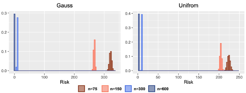
Figure 1. Excess risks of posterior samples in Scenario (i) and (ii). The left (right) figure shows histograms of excess risks of $n=75,\ 150,\ 300,$ and $600$ for scenario (i) and the right shows ones for scenario (ii).

5.3. Experiment of posterior approximation

Here, we confirm the result of Theorem 3 by visualizing the posterior sample from MCMC and samples from $N_{tr}(\bar{\bm{\theta}},\ddot{\Sigma})$. The blue dots (red dots) in Figure 2 represent MCMC samples (approximate samples) of the first two parameters of $\bm{\theta}$, in Scenario 1 (Scenario 2) with $n=150$ $(300,600)$ if a panel is in the top row (bottom row) and the left column (center column, right column). The plots with $n=75$ are not shown here because the variances are large and the two distributions are far apart, although the other panels are sufficient for discussing the results. In both scenarios, the two types of samples overlap more as the sample size increases. This corresponds to the fact that the distance between the posterior distribution and its approximate distribution converges to zero, as shown in Theorem 3. The sample variances of both distributions also decrease. This is because, for the posterior distribution, the uncertainty (variance) naturally decreases as the information (sample) increases, and, for the approximate distribution, the expectation of $\ddot{\Sigma}$ equals $\sigma^{2}\Sigma/n$, which is inversely proportional to the sample size. Additionally, the distribution of each coordinate resembles a bell-shaped, symmetrical distribution, supporting the validity of Gaussian approximation.

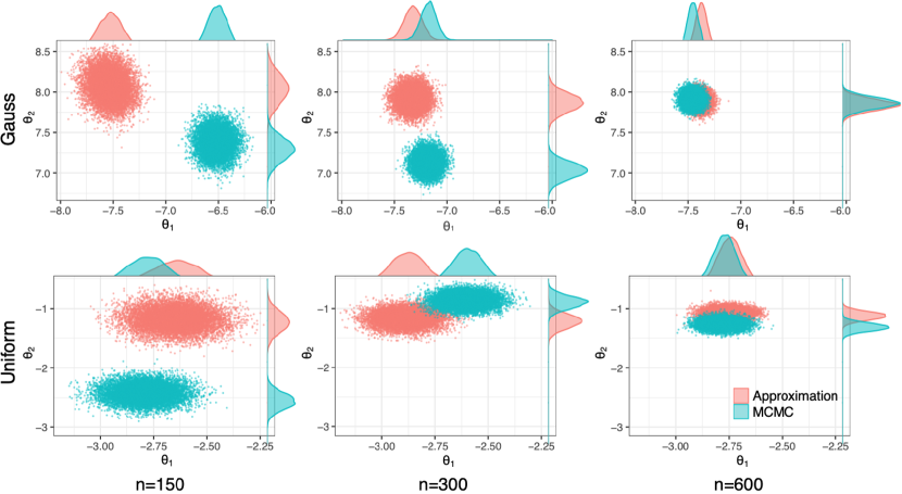
Figure 2. Blue dots (red dots) show MCMC samples (approximate samples) of the top two parameters of $\bm{\theta}$, in Scenario 1 (Scenario 2) with $n=150$ $(300,600)$ if a panel is in the top row (bottom row) and the left column (center column, right column).

6. Discussion

In this paper, we address an over-parameterized Bayesian linear regression problem. Usually, the assumption that the parameters are sparse is introduced for such problems, but we do not stick to this assumption and consider a non-sparse situation. The posterior estimator tends to be unstable in this situation, but we have devised an effective prior distribution, showed the consistency of its posterior estimator, and described a Gaussian approximation of its posterior distribution. The numerical experiments also evince that our theoretical results are valid. To conclude, we present the contributions of our findings from two different perspectives.

6.1. Moden overparametrized theory

In the realm of high-dimensional linear regression, a phenomenon known as the benign overfitting of the minimum norm interpolator has been observed. An analogy can be drawn between the phenomenon and the current result. Specifically, the interpolator is defined as an estimator with the smallest norm among the quantities that make the quadratic loss zero. In our approach, the likelihood function serves to control the quadratic loss, and the prior distribution plays a role in regulating the norm. Our method provides uncertainty quantification by taking advantage of the posterior distribution and improves the utility of the over-parameterized model. Furthermore, we contribute to eliminating the sub-Gaussianity of covariates, which was imposed by earlier studies [10, 45, 28]. Although random variables with thin-tailed are more likely to achieve posterior contraction (benign overfitting), we demonstrate that thicker-tailed distributions can also achieve this objective. There is some concern that the contraction rate may be slow depending on the setting, but we leave this for future work, which may be improved depending on the proof strategy.

6.2. Bayesian high-dimensional theory

The asymptotic behavior of high-dimensional Bayesian methods has been studied. [23] demonstrated that, when $p^{4}\log p<n$ is satisfied, posterior contractions and normal approximations hold. However, in the theory of an excess number of parameters, one could either establish a posterior contraction and a normal approximation (or a similar property) under the sparsity assumption [18, 39], or show the property with respect to a single parameter [57, 54]. These results indicate the challenges in obtaining the properties of high-dimensional parameters from a relatively small amount of data. Our contribution is to present the conditions and prior distributions that allow posterior contraction and normal approximation for non-sparse over-parameterized models by exploiting the intrinsically low dimensionality of covariates. The model considered in this study is typical and does not allow for more flexible structures or non-iid situations. Nonetheless, owing to this simplicity, we have been able to elucidate its theoretical properties successfully. Moreover, since the investigation of more complex and adaptive methods often builds upon the analyses of simple methods, the findings of this study could serve as a foundation for further research.

Appendix A Proof of Theorem 1 and Theorem 2

Here, we only prove Theorem 2. Theorem 1 holds naturally, since it only requires the substitution of specific values for $\rho_{n}$, which is dealt with in Theorem 2.

In view of Theorem 2.1 of [21], the statement of Theorem 2 holds if the following three conditions are satisfied for sufficiently large $n$:

$$\log\mathcal{N}(\varepsilon_{n},\mathcal{P}_{n},(d_{1},d_{2}))\leq n\varepsilon_{n}^{2},$$ (4)

$$\Pi(\mathcal{P}\setminus\mathcal{P}_{n})\leq\exp(-(C+4)n\varepsilon_{n}^{2}),$$ (5)

$$\Pi\left(\left\{\bm{\theta},\sigma^{2}:K(g^{*},g)\leq\varepsilon_{n}^{2},V(g^{*},g)\leq\varepsilon_{n}^{2}\right\}\right)\geq\exp(-Cn\varepsilon_{n}^{2}).$$ (6)

where $d_{1}(\cdot,\cdot):\mathbb{R}\times\mathbb{R}\to\mathbb{R}$ and $d_{2}(\cdot,\cdot):\mathbb{R}^{p}\times\mathbb{R}^{p}\to\mathbb{R}$ are distances induced by norms $\|\cdot\|_{1}$ and $\|\cdot\|_{\Sigma}$, $g$ denotes the joint density of $\{\bm{x},y\}$ under a generic value of the parameter $(\bm{\theta},\sigma)$ and $g^{*}$ denotes the density under $(\bm{\theta}^{*},\sigma^{*})$.

A.1. Condition (4)

We decompose the covering number in (4). We have an inequality

$$\log\mathcal{N}(\varepsilon_{n},\mathcal{P}_{n},(d_{1},d_{2}))\leq\log\mathcal{N}(\varepsilon_{n},\mathcal{P}_{n}^{1},|\cdot|)+\log\mathcal{N}(\varepsilon_{n},\mathcal{P}_{n}^{2},\|\cdot\|_{\Sigma}).$$

The first term is bounded by $\log(n/\varepsilon_{n})$ because the length of interval $\mathcal{P}_{n}^{1}$ is $2n$, and $n/\varepsilon_{n}$ open intervals of length $2\varepsilon_{n}$ are sufficient to cover it. Then, we focus on the second term.

From Lemma 1 and some properties of covering number [46], we have

$$\log\mathcal{N}(\varepsilon_{n},\mathcal{P}_{n}^{2},\|\cdot\|_{\Sigma}) =\log\mathcal{N}(\varepsilon_{n},\Sigma^{1/2}\mathcal{P}_{n}^{2},\|\cdot\|_{2})$$

$$\leq\log\mathcal{N}(\varepsilon_{n}/2,\Sigma_{1}^{1/2}\mathcal{P}_{n}^{2},\|\cdot\|_{2})+\log\mathcal{N}(\varepsilon_{n}/2,\Sigma_{2}^{1/2}\mathcal{P}_{n}^{2},\|\cdot\|_{2})$$

$$=\log\underbrace{\mathcal{N}(\varepsilon_{n}/2,\mathcal{P}_{n}^{2},\|\cdot\|_{\Sigma_{1}})}_{=:\mathcal{N}_{1}}+\log\underbrace{\mathcal{N}(\varepsilon_{n}/2,\Sigma_{2}^{1/2}\mathcal{P}_{n}^{2},\|\cdot\|_{2})}_{=:\mathcal{N}_{2}}.$$

We will show the two terms separately. The two bounds are valid for any $k^{*}$ on the support of $\pi$. To simplify notation, we substitute $\varepsilon_{n}/2$ for $\varepsilon_{n}$. Note that this substitution does not affect the following result.

A.1.1. bound $\mathcal{N}_{1}$

We first develop a bound $\log\mathcal{N}_{1}\leq n\varepsilon_{n}^{2}/2$. Define an orthogonal matrix $U=(\bm{v}_{1},...,\bm{v}_{p})\in\mathbb{R}^{p\times p}$, where $\bm{v}_{j}$ are eigenvectors defined in Section 2. For any $\bm{h}_{1},\bm{h}_{2}\in\mathbb{R}^{p}$, it holds that

$$(\bm{h}_{1}-\bm{h}_{2})^{\top}\Sigma_{1}(\bm{h}_{1}-\bm{h}_{2}) =(\bm{h}_{1}-\bm{h}_{2})^{\top}U\mathrm{diag}(\lambda_{1},\ldots\lambda_{k^{*}},0\ldots,0)U^{\top}(\bm{h}_{1}-\bm{h}_{2})$$

$$=(\bm{h}_{1}^{\prime}-\bm{h}_{2}^{\prime})^{\top}\mathrm{diag}(\lambda_{1},\ldots\lambda_{k^{*}},0\ldots,0)(\bm{h}_{1}^{\prime}-\bm{h}_{2}^{\prime}),\ \ \ \ \bm{h}_{1}^{\prime},\bm{h}_{2}^{\prime}\in U^{\top}\mathbb{R}^{p}.$$

This implies that if $k^{*}$ components of two elements $\bm{h}_{1}^{\prime},\bm{h}_{2}^{\prime}$ in $U^{\top}\mathbb{R}^{p}(=\mathbb{R}^{p})$ are same, the distance $(\bm{h}_{1}^{\prime}-\bm{h}_{2}^{\prime})^{\top}\mathrm{diag}(\lambda_{1},\ldots\lambda_{k^{*}},0\ldots,0)(\bm{h}_{1}^{\prime}-\bm{h}_{2}^{\prime})$ is zero. Hence, $p-k^{*}$ components of $U^{\top}\mathbb{R}^{p}(=\mathbb{R}^{p})$ can be ignored in this covering discussion and it holds that

$$\mathcal{N}_{1}=\mathcal{N}(\varepsilon_{n},\{\bm{\theta}\in\mathbb{R}^{k^{*}}:\|\bm{\theta}\|_{2}\leq H_{n}\},\|\cdot\|_{\check{\Sigma}_{1}}),$$

where $\check{\Sigma}_{1}=\mathrm{diag}(\lambda_{1},\ldots\lambda_{k^{*}})$. Because relations $\{\bm{\theta}\in\mathbb{R}^{k^{*}}:\|\bm{\theta}\|_{2}\leq H_{n}\}\subset[-H_{n},H_{n}]^{k^{*}}$ and $\mathcal{N}_{1}\leq M(\varepsilon_{n},\{\bm{\theta}\in\mathbb{R}^{k^{*}}:\|\bm{\theta}\|_{2}\leq H_{n}\},\|\cdot\|_{\check{\Sigma}_{1}})$ holds [50], it is sufficient to prove $\log\mathcal{M}:=\log\mathcal{M}(\varepsilon_{n},[-H_{n},H_{n}]^{k^{*}},\|\cdot\|_{\check{\Sigma}_{1}})\leq n\varepsilon_{n}^{2}/2$.

Let $\{\beta_{1},\ldots,\beta_{M}\}$ be an $\varepsilon_{n}$ packing of $[-H_{n},H_{n}]^{k^{*}}$. It holds

$$\bigcup_{j=1}^{M}\left\{\beta_{j}+\frac{\varepsilon_{n}}{2}\mathbb{B}_{1}\right\}\subset[-H_{n},H_{n}]^{k^{*}}+\frac{\varepsilon_{n}}{2}\mathbb{B}_{1},$$

where $\mathbb{B}_{1}$ is an unit ball with the distance $\|\cdot\|_{\check{\Sigma}_{1}}$. Let $\mathrm{vol}(\cdot)$ denote the Lebesgue measure of an object in Euclid space. We have

$$\mathcal{M} \mathrm{vol}(\frac{\varepsilon_{n}}{2}\mathbb{B}_{1})\leq\mathrm{vol}\left([-H_{n},H_{n}]^{k^{*}}+\frac{\varepsilon_{n}}{2}\mathbb{B}_{1}\right).$$

Therefore, we have, with some constant $c_{2}>0$,

$$\mathcal{M} \leq\frac{\mathrm{vol}\left([-H_{n},H_{n}]^{k^{*}}+\frac{\varepsilon_{n}}{2}\mathbb{B}_{1}\right)}{\mathrm{vol}\left(\frac{\varepsilon_{n}}{2}\mathbb{B}_{1}\right)}$$

$$=\frac{\mathrm{vol}\left(\frac{2}{\varepsilon_{n}}[-H_{n},H_{n}]^{k^{*}}+\mathbb{B}_{1}\right)}{\mathrm{vol}\left(\mathbb{B}_{1}\right)}$$

$$\leq\frac{\Gamma(\frac{k^{*}}{2}+1)\prod_{j=1}^{k^{*}}\left(\frac{4H_{n}}{\varepsilon_{n}}+\frac{1}{\sqrt{\lambda_{j}}}\right)}{\pi^{k^{*}/2}\prod_{j=1}^{k^{*}}\left(\frac{1}{\sqrt{\lambda_{j}}}\right)}$$

$$\leq\Gamma\left(\frac{k^{*}}{2}+1\right)\prod_{j=1}^{k^{*}}\left(\frac{4H_{n}\sqrt{\lambda_{j}}}{\sqrt{\pi}\varepsilon_{n}}+1\right)$$

$$\leq c_{2}\Gamma\left(\frac{k^{*}}{2}+1\right)\left(\frac{4H_{n}\sqrt{\lambda_{1}}}{\varepsilon_{n}}\right)^{k^{*}}$$

The second equality follows the volume of $k^{*}$-dimensional ellipsoid [e.g., 53]. Then we get, with some constant $c_{3}>0$,

$$\log\mathcal{N}_{1}\leq k^{*}\log\left(\frac{4c_{2}H_{n}\sqrt{\lambda_{1}}}{\varepsilon_{n}}\right)+\log\Gamma\left(\frac{k^{*}}{2}+1\right)\leq k^{*}\log\left(\frac{4c_{2}H_{n}\sqrt{\lambda_{1}}}{\varepsilon_{n}}\right)+\frac{k^{*}}{2}\log\frac{k^{*}}{2}\leq c_{3}n\varepsilon_{n}^{2}/2,$$

where the second inequality holds from Stirling’s approximation and the last inequality holds from Assumption 2-[3]. At last, we can bound the covering number $\mathcal{N}_{1}$ by the truncation level $k^{*}$ through bounding the volume of the hyper-cube.

A.1.2. bound $\mathcal{N}_{2}$

Next, we consider $\mathcal{N}_{2}$. It holds, from the Sudakov minoration [e.g., 51, Section 5.5],

$$\log\mathcal{N}(\varepsilon_{n},\Sigma_{2}^{1/2}\mathcal{P}_{n}^{2},\|\cdot\|_{2})\leq\varepsilon_{n}^{-2}\mathbb{E}^{2}\sup_{\bm{h}\in\Sigma_{2}^{1/2}\mathcal{P}_{n}^{2}}\bm{h}^{\top}\bm{Z},$$

where $\bm{Z}\sim N(\bm{0},I_{p})$. Define $\bm{Z}^{\prime}:=\Sigma_{2}^{1/2}\bm{Z}$ Since

$$\mathbb{E}\sup_{\bm{h}\in\Sigma_{2}^{1/2}\mathcal{P}_{n}^{2}}\bm{h}^{\top}\bm{Z} \leq\mathbb{E}\sup_{\bm{h}\in\mathcal{P}_{n}^{2}}\bm{h}^{\top}\bm{Z}^{\prime}$$

$$=H_{n}\mathbb{E}\sup_{\bm{h}\in B_{2}}\bm{h}^{\top}\bm{Z}^{\prime}=H_{n}\mathbb{E}\|\bm{Z}^{\prime}\|_{2}\leq H_{n}\sqrt{\mathbb{E}\|\bm{Z}^{\prime}\|^{2}_{2}}\ \ \ (\because\mathrm{Jensen})$$

$$=H_{n}\sqrt{\sum_{i=1}^{p}\operatorname{Var}(Z^{\prime}_{i})}=H_{n}\sqrt{\sum_{i=k^{*}+1}^{p}\lambda_{i}},$$

Hence, $\log\mathcal{N}(\varepsilon_{n},\mathcal{P}_{n}^{2},\|\cdot\|_{\Sigma_{2}})\leq(H_{n}^{2}/\varepsilon_{n}^{2})\sum_{i=k^{*}+1}^{p}\lambda_{i}$ holds. From Assumption 2-[2], $\log\mathcal{N}_{2}<n\varepsilon_{n}^{2}/2.$ As an interpretation of $\mathcal{N}_{2}$: Although the mapped space is a high ($p-k^{*}$) dimension, complexity is small because the eigenvalue of the map is small.

A.2. Condition (5)

It holds that

$$\Pi(\mathcal{P}\setminus\mathcal{P}_{n})\leq\Pi_{\bm{\theta}}(\|\bm{\theta}\|_{2}\geq H_{n})+\Pi_{\sigma}(\sigma^{2}\leq n^{-1})+\Pi_{\sigma}(\sigma^{2}\geq n).$$

Since the prior for $\sigma^{2}$ is Inverse Gaussian, tail decay is exponentially fast and $\Pi(\sigma^{2}\leq n^{-1})$ and $\Pi(\sigma^{2}\geq n)$ are bounded by $e^{-nC_{\mathrm{IG}}}(<e^{-n\varepsilon_{n}^{2}})$ with some constant $C_{\mathrm{IG}}$.

Then, we consider the first term. For $\widehat{\Sigma}_{1}$, there exists a unitary matrix $\widehat{U}$ such that $\widehat{U}^{\top}\widehat{\Sigma}_{1}\widehat{U}$ is diagonal. With this $\widehat{U}$, we define $\bm{u}=\widehat{U}^{\top}\bm{\theta}$ and $\widetilde{\Sigma}_{1}=\widehat{U}^{\top}\widehat{\Sigma}_{1}\widehat{U}$. Then, we have the following prior for the rotated parameter $\bm{u}$:

$$\Pi_{\bm{\theta}}(\bm{u})=\frac{\exp\left\{-\bm{u}^{\top}\widetilde{\Sigma}_{1}^{\dagger}\bm{u}\right\}\textbf{1}\{\|\bm{u}^{\prime}\|_{2}\leq R\}}{\int\exp\left\{-\bm{u}^{\prime\top}\widetilde{\Sigma}_{1}^{\dagger}\bm{u}^{\prime}\right\}\textbf{1}\{\|\bm{u}^{\prime}\|_{2}\leq R\}d\bm{u}^{\prime}}.$$

Since $\widehat{\Sigma}_{1}$ is a matrix with its rank $k^{*}$, lower $p-k^{*}$ rows of $\widetilde{\Sigma}_{1}$ are zeroes. When $\widehat{\Sigma}_{1}$ is a rank $k$ matrix, we denote $\bm{u}$ as $\bm{u}^{(k)}$. Then we have

$$\Pi_{\bm{\theta}}(\|\bm{\theta}\|^{2}_{2}>H_{n}^{2})=\sum_{k^{*}=L_{k}}^{U_{k}}\pi(k^{*})\Pi_{\bm{\theta}}(\|\bm{u}^{(k^{*})}\|^{2}_{2}>H_{n}^{2})=\sum_{k^{*}=L_{k}}^{U_{k}}\pi(k^{*})\Pi^{(k^{*})}_{\bm{\theta}}(\|\bm{u}_{1}^{(k^{*})}\|_{2}^{2}>H_{n}^{2}),$$

where $\bm{u}_{1}^{(k^{*})}$ is a $k^{*}$-dimensional vector composed of the first $k^{*}$ elements of $\bm{u}^{(k^{*})}$, $\widetilde{\Sigma}_{1}^{(k^{*})}:=\mathrm{diag}(\widehat{\lambda}_{1},...,\widehat{\lambda}_{k^{*}})$, and

$$\Pi^{(k^{*})}_{\bm{\theta}}(\bm{u}_{1}^{(k^{*})})\propto\exp\left\{-\bm{u}^{(k^{*})\top}_{1}\widetilde{\Sigma}_{1}^{(k^{*})-1}\bm{u}^{(k^{*})}_{1}\right\}\textbf{1}\{\|\bm{u}_{1}^{(k^{*})}\|_{2}\leq R\}.$$

It is sufficient to prove that

$$\sum_{k^{*}=L_{k}}^{U_{k}}\pi(k^{*})\Pi_{\bm{\theta}}^{(k^{*})}(\|\bm{u}_{1}^{(k^{*})}\|_{2}>H_{n})\leq\exp(-Cn\varepsilon_{n}^{2}).$$

We fix $k^{*}$ and examine $\Pi^{\prime}_{\bm{\theta}}(\|\bm{u}_{1}\|_{2}>H_{n})$ with $\bm{u}_{1}=\bm{u}_{1}^{(k^{*})}$ and $\Pi^{\prime}_{\bm{\theta}}=\Pi_{\bm{\theta}}^{(k^{*})}$. Let $N_{1/2}$ be a $1/2$-minimal cover of a $k^{*}$-dimensional Euclidean unit ball $B_{2}$ in $\|\cdot\|_{2}$. We have

$$\|\bm{u}_{1}\|_{2} =\max_{\bm{h}\in B_{2}}\bm{h}^{\top}\bm{u}_{1}\leq\max_{\bm{h}\in N_{1/2}}\bm{h}^{\top}\bm{u}_{1}+\max_{\bm{h}\in\frac{1}{2}B_{2}}\bm{h}^{\top}\bm{u}_{1}\leq\max_{\bm{h}\in N_{1/2}}\bm{h}^{\top}\bm{u}_{1}+\frac{1}{2}\|\bm{u}_{1}\|_{2},$$

that is, $\|\bm{u}_{1}\|_{2}\leq 2\max_{\bm{z}\in N_{1/2}}\bm{z}^{\top}\bm{u}_{1}$. With Gaussian measure $\check{\Pi}_{\bm{\theta}}(\bm{u}_{1}):=N(\bm{0},\mathrm{diag}(\widehat{\lambda}_{1},...,\widehat{\lambda}_{k^{*}}))$, we obtain

$$\Pi^{\prime}_{\bm{\theta}}(\|\bm{u}_{1}\|_{2}>H_{n}) \leq\Pi^{\prime}_{\bm{\theta}}\left(\max_{\bm{z}\in N_{1/2}}\bm{z}^{\top}\bm{u}_{1}>H_{n}/2\right)\leq|N_{1/2}|\max_{\bm{z}\in N_{1/2}}\Pi^{\prime}_{\bm{\theta}}(\bm{z}^{\top}\bm{u}_{1}>H_{n}/2)$$

$$\leq|N_{1/2}|\max_{\bm{z}\in N_{1/2}}\check{\Pi}_{\bm{\theta}}(\bm{z}^{\top}\bm{u}_{1}>H_{n}/2)\lesssim|N_{1/2}|\exp\left(-\frac{H_{n}^{2}}{8\widehat{\lambda}_{1}}\right).$$ (7)

The third inequality holds since the tail probability of Gaussian is larger than that of truncated Gaussian. The last inequality holds by Chernoff bound since $\bm{z}^{\top}\bm{u}_{1}$ is sub-Gaussian with parameter $\widehat{\lambda}_{1}$. Let $\bm{Z}\sim N(\bm{0},I_{k^{*}})$. We have

$$|N_{1/2}| =\mathcal{N}(\frac{1}{2},B_{2},\|\cdot\|_{2})\stackrel{{\scriptstyle\mathrm{Sudakov}}}{{\leq}}\exp\left(2^{2}\mathbb{E}^{2}\sup_{\bm{h}\in B_{2}}\bm{h}^{\top}\bm{Z}\right)\leq\exp(4\mathbb{E}^{2}\|\bm{Z}\|_{2})$$

$$\stackrel{{\scriptstyle\mathrm{Jensen}}}{{\leq}}\exp(4\mathbb{E}\|\bm{Z}\|^{2}_{2})=\exp\left(4\sum_{j=1}^{k^{*}}\operatorname{Var}(Z_{j})\right)=\exp(4k^{*}).$$ (8)

From (A.2) and (A.2), we obtain $\Pi^{\prime}_{\bm{\theta}}(\|\bm{u}_{1}\|_{2}>H_{n})\leq\exp\left(4k^{*}-\frac{H_{n}^{2}}{8\widehat{\lambda}_{1}}\right).$ Then we have

$$\sum_{k^{*}=L_{k}}^{U_{k}}\pi(k^{*})\Pi^{\prime}_{\bm{\theta}}(\|\bm{u}_{1}^{(k^{*})}\|_{2}>H^{2}_{n}) \leq\sum_{k^{*}=L_{k}}^{U_{k}}\pi(k^{*})\exp\left(4k^{*}-\frac{H_{n}^{2}}{8\widehat{\lambda}_{1}}\right)$$

$$\leq\sum_{k^{*}=L_{k}}^{U_{k}}\pi(k^{*})\exp\left(4k^{*}-\frac{\lambda_{1}}{\widehat{\lambda}_{1}}\frac{H_{n}^{2}}{8\lambda_{1}}\right).$$ (9)

We have

$$\left|\frac{\widehat{\lambda}_{1}}{\lambda_{1}}-1\right|\leq\frac{|\widehat{\lambda}_{1}-\lambda_{1}|}{\lambda_{1}}=\frac{\|\widehat{\Sigma}-\Sigma\|_{\mathrm{op}}}{\|\Sigma\|_{\mathrm{op}}}\leq\rho_{n}=o(1)$$

with probability at least $1-\ell_{n}$ from Assumption 3. Then, we obtain, with probability at least $1-\ell_{n}$,

$$\sum_{k^{*}=L_{k}}^{U_{k}}\pi(k^{*})\Pi^{\prime}_{\bm{\theta}}(\|\bm{u}_{1}^{(k^{*})}\|_{2}>H_{n}) \leq\sum_{k^{*}=L_{k}}^{U_{k}}\pi(k^{*})\exp\left(4k^{*}-(1-\rho_{n})\frac{H_{n}^{2}}{8\lambda_{1}}\right)$$

$$\leq(U_{k}-L_{k}+1)\exp\left(-L_{k}^{-2}-(1-\rho_{n})\frac{H_{n}^{2}}{8\lambda_{1}}\right).$$

The last inequality holds from the definition of $\pi(k^{*}).$ By Assumption 2-[3], the last term is bounded by $\exp(-n\varepsilon_{n}^{2})$.

A.3. Condition (6)

Since the Kullback-Leibler divergence is rewritten as

$$K(g^{*},g) =\int_{\bm{x}}\int_{y}g^{*}(y,\bm{x})\log(g^{*}(y,\bm{x})/g(y,\bm{x}))dyd\bm{x}$$

$$=\int_{\bm{x}}\int_{y}g^{*}(y\mid\bm{x})g^{*}(\bm{x})\{\log(g^{*}(y\mid\bm{x})/g(y\mid\bm{x}))+\log(g^{*}(\bm{x})/g(\bm{x}))\}dyd\bm{x}$$

$$=\int_{\bm{x}}g^{*}(\bm{x})\int_{y}g^{*}(y\mid\bm{x})\log(g^{*}(y\mid\bm{x})/g(y\mid\bm{x}))dyd\bm{x}$$

$$=\mathbb{E}_{\bm{x}}\left[\frac{1}{2}\frac{{\sigma^{*}}^{2}}{\sigma^{2}}-\frac{1}{2}\log(\frac{{\sigma^{*}}^{2}}{\sigma^{2}})-\frac{1}{2}+\frac{1}{2}\frac{{\|\bm{x}^{\top}\bm{\theta}^{*}-\bm{y}\|_{2}^{2}}}{\sigma^{2}}-\frac{1}{2}\frac{{\|\bm{x}^{\top}\bm{\theta}-\bm{y}\|_{2}^{2}}}{\sigma^{2}}\right]$$

$$\leq\mathbb{E}_{\bm{x}}\left[\frac{1}{2}\frac{{\sigma^{*}}^{2}}{\sigma^{2}}-\frac{1}{2}\log(\frac{{\sigma^{*}}^{2}}{\sigma^{2}})-\frac{1}{2}+\frac{1}{2}\frac{{\|\bm{x}^{\top}\bm{\theta}^{*}-\bm{x}^{\top}\bm{\theta}\|_{2}^{2}}}{\sigma^{2}}\right]$$

$$=\frac{1}{2}\frac{{\sigma^{*}}^{2}}{\sigma^{2}}-\frac{1}{2}\log(\frac{{\sigma^{*}}^{2}}{\sigma^{2}})-\frac{1}{2}+\frac{1}{2}\frac{{\|\bm{\theta}^{*}-\bm{\theta}\|_{\Sigma}^{2}}}{\sigma^{2}},$$

and the Kullback-Leibler variation is also written as

$$V(g^{*},g) =\frac{1}{2}\frac{{\sigma^{*}}^{4}}{\sigma^{4}}-\frac{{\sigma^{*}}^{2}}{\sigma^{2}}+\frac{1}{2}+\frac{{\sigma^{*}}^{2}}{\sigma^{2}}\frac{\|\bm{\theta}^{*}-\bm{\theta}\|^{2}_{\Sigma}}{\sigma^{2}}.$$

Hence, it holds that

$$\Pi\left(\left\{\bm{\theta},\sigma^{2}:K(g^{*},g)\leq\varepsilon_{n}^{2},V(g^{*},g)\leq\varepsilon_{n}^{2}\right\}\right)\geq\Pi\left(\mathcal{B}_{2}\mid\mathcal{B}_{1}\right)\Pi\left(\mathcal{B}_{1}\right),$$ (10)

where

$$\mathcal{B}_{1} =\Big{\{}\sigma^{2}:\frac{{\sigma^{*}}^{2}}{\sigma^{2}}-\log\Big{(}\frac{{\sigma^{*}}^{2}}{\sigma^{2}}\Big{)}-1\leq\varepsilon_{n}^{2},\quad\frac{{\sigma^{*}}^{4}}{\sigma^{4}}-\frac{2{\sigma^{*}}^{2}}{\sigma^{2}}+1\leq\varepsilon_{n}^{2}\Big{\}},$$

$$\mathcal{B}_{2} =\Big{\{}(\bm{\beta},\sigma^{2}):\frac{1}{2}\frac{\|\bm{\theta}^{*}-\bm{\theta}\|^{2}_{{\Sigma}}}{\sigma^{2}}\leq\varepsilon_{n}^{2},\quad\frac{{\sigma^{*}}^{2}}{\sigma^{2}}\frac{\|\bm{\theta}^{*}-\bm{\theta}\|^{2}_{{\Sigma}}}{\sigma^{2}}\leq\frac{\varepsilon_{n}^{2}}{2}\Big{\}}.$$

A.3.1. Divergence of $\sigma^{2}$

We first discuss $\Pi\left(\mathcal{B}_{1}\right)$. Since the logarithm has Maclaurin series $\log(1+x)=x-\frac{x^{2}}{2}+o(x^{2})$, we obtain

$$\frac{{\sigma^{*}}^{2}}{\sigma^{2}}-\log\left(1+\frac{{\sigma^{*}}^{2}}{\sigma^{2}}-1\right)-1 =\frac{{\sigma^{*}}^{2}}{\sigma^{2}}-\left\{\frac{{\sigma^{*}}^{2}}{\sigma^{2}}-1-\frac{1}{2}\left(\frac{{\sigma^{*}}^{2}}{\sigma^{2}}-1\right)^{2}\right\}-1+o\left(\left(\frac{{\sigma^{*}}^{2}}{\sigma^{2}}-1\right)^{2}\right)$$

$$=\frac{1}{2}\left(\frac{{\sigma^{*}}^{4}}{\sigma^{4}}-\frac{2{\sigma^{*}}^{2}}{\sigma^{2}}+1\right)+o\left(\left(\frac{{\sigma^{*}}^{2}}{\sigma^{2}}-1\right)^{2}\right).$$

If we denote $\Delta=\frac{{\sigma^{*}}^{2}}{\sigma^{2}}-1$, $\Pi(\mathcal{B}_{1})=\Pi(\Delta^{2}/2+o(\Delta^{2})\leq\varepsilon_{n}^{2},\Delta^{2}\leq\varepsilon_{n}^{2}).$ The second condition $\Delta^{2}\leq\varepsilon_{n}^{2}(\to 0)$ implies $\Delta^{2}/2\leq\varepsilon_{n}^{2}/2$ holds and $o(\Delta^{2})\leq\varepsilon_{n}^{2}/2$ holds asymptotically. Hence $\Pi(\mathcal{B}_{1})=\Pi(\Delta\leq\varepsilon_{n})$. Hence, to bound $\Pi(\mathcal{B}_{1})$, it is sufficient to evaluate

$$\Pi\left(\sigma^{2}:\left|\frac{{\sigma^{*}}^{2}}{\sigma^{2}}-1\right|\leq\varepsilon_{n}\right).$$

Since the prior distribution of $\sigma^{2}$ follows the inverse Gaussian distribution, we consider the transform $\widetilde{\sigma}=\sigma^{-2}$ and obtain

$$\Pi\left(\sigma^{2}:\left|\frac{1}{\sigma^{2}}-\frac{1}{{\sigma^{*}}^{2}}\right|\leq\frac{\varepsilon_{n}}{{\sigma^{*}}^{2}}\right)$$

$$\gtrsim\int_{{\sigma^{*}}^{-2}-{\sigma^{*}}^{-2}\varepsilon_{n}}^{{\sigma^{*}}^{-2}+{\sigma^{*}}^{-2}\varepsilon_{n}}\widetilde{\sigma}^{-\frac{1}{2}}e^{-\widetilde{\sigma}}e^{-\frac{1}{\widetilde{\sigma}}}d\widetilde{\sigma}$$

$$\gtrsim 2{\sigma^{*}}^{-2}\varepsilon_{n}\left({\sigma^{*}}^{-2}+{\sigma^{*}}^{-2}\varepsilon_{n}\right)^{-\frac{1}{2}}\exp\left(-{\sigma^{*}}^{-2}-{\sigma^{*}}^{-2}\varepsilon_{n}\right)\exp\left(\frac{-1}{{\sigma^{*}}^{-2}-{\sigma^{*}}^{-2}\varepsilon_{n}}\right)$$

$$\approx\varepsilon_{n}.$$ (11)

The first inequality follows the transformation $\widetilde{\sigma}=\sigma^{-2}$. In the second inequality, $2{\sigma^{*}}^{-2}\varepsilon_{n}$ is the length of the integral interval. $({\sigma^{*}}^{-2}+{\sigma^{*}}^{-2}\varepsilon_{n})^{-1/2}$ is the minimum value of $\widetilde{\sigma}^{-1/2}$. Other terms are also minimum values of integrands within the integral interval.

A.3.2. Divergence of $\bm{\theta}$

From the former section, it is shown that $\sigma$ is close to constant $\sigma^{*}$ in $\Pi$. Hence, to bound the probability of event $\mathcal{B}_{2}$ given $\mathcal{B}_{1}$, it is sufficient to evaluate

$$\Pi_{\bm{\theta}}(\{\bm{\theta}\in\mathbb{R}^{p}:\|\bm{\theta}-\bm{\theta}^{*}\|_{\Sigma}^{2}\geq\varepsilon_{n}^{2}\}).$$

Because $\|\bm{\theta}-\bm{\theta}^{*}\|_{\Sigma}^{2}=(\bm{\theta}-\bm{\theta}^{*})^{\top}(\Sigma-\widehat{\Sigma})(\bm{\theta}-\bm{\theta}^{*})+(\bm{\theta}-\bm{\theta}^{*})^{\top}\widehat{\Sigma}(\bm{\theta}-\bm{\theta}^{*})\leq(\bm{\theta}-\bm{\theta}^{*})^{\top}(\lambda_{1}\rho_{n}I+\widehat{\Sigma})(\bm{\theta}-\bm{\theta}^{*})$, the rotation by $\widehat{U}$ yields

$$\|\bm{\theta}-\bm{\theta}^{*}\|_{\Sigma}^{2}\leq(\bm{u}-\bm{u}^{*})^{\top}\mathrm{diag}(\lambda_{1}\rho_{n}+\widehat{\lambda}_{1},\lambda_{1}\rho_{n}+\widehat{\lambda}_{2}\ldots,\lambda_{1}\rho_{n}+\widehat{\lambda}_{k^{*}})(\bm{u}-\bm{u}^{*}).$$

Hence, we bound the target probability as

$$\Pi_{\bm{\theta}}(\{\bm{\theta}\in\mathbb{R}^{p}:\|\bm{\theta}-\bm{\theta}^{*}\|_{\Sigma}^{2}\geq\varepsilon_{n}^{2}\})\leq\sum_{k^{*}=L_{k}}^{U_{k}}\pi(k^{*})\Pi_{\bm{\theta}}(\{\bm{u}\in\mathbb{R}^{p}:\|\bm{u}^{(k^{*})}-\bm{u}^{*}\|_{\grave{\Sigma}}^{2}\geq\varepsilon_{n}^{2}\}),$$

where $\grave{\Sigma}:=\mathrm{diag}(\widetilde{\lambda}_{1},\ldots,\widetilde{\lambda}_{p}):=\mathrm{diag}(\lambda_{1}\rho_{n}+\widehat{\lambda}_{1},\ldots,\lambda_{1}\rho_{n}+\widehat{\lambda}_{p})$.

We fix $k^{*}$ and examine $\Pi^{\prime}_{\bm{\theta}}(\{\bm{u}\in\mathbb{R}^{p}:\|\bm{u}-\bm{u}^{*}\|_{\grave{\Sigma}}^{2}\geq\varepsilon_{n}^{2}\}),$ with $\bm{u}=\bm{u}^{(k^{*})}$. Note that, on measure $\Pi_{\bm{\theta}}(\bm{u})$, the lower $p-k^{*}$ elements of $\bm{u}$ is zeroes, and hence we obtain

$$\|\bm{u}-\bm{u}^{*}\|_{\grave{\Sigma}}^{2}\leq\|\bm{u}_{1}-\bm{u}^{*}_{1}\|_{\grave{\Sigma}^{(k^{*})}}^{2}+\widetilde{\lambda}_{k^{*}}\|\bm{u}^{*}_{2}\|_{2}^{2}.$$

where $\bm{u}_{1}$ and $\bm{u}^{*}_{1}$ are $k^{*}$-dimensional vectors composed of the first $k^{*}$ elements of $\bm{u}$ and $\bm{u}^{*}$, $\bm{u}^{*}_{2}$ is remaining part of $\bm{u}^{*}$, and $\grave{\Sigma}^{(k^{*})}=\mathrm{diag}(\widetilde{\lambda}_{1},\ldots,\widetilde{\lambda}_{k^{*}})$. Then, we rewrite the tail probability as

$$\Pi_{\bm{\theta}}\left(\left\{\bm{u}\in\mathbb{R}^{p}:\|\bm{u}-\bm{u}^{*}\|_{\grave{\Sigma}}^{2}\geq\varepsilon_{n}^{2}\right\}\right)\leq\Pi_{1}\left(\left\{\bm{u}_{1}\in\mathbb{R}^{k^{*}}:\|\bm{u}_{1}-\bm{u}^{*}_{1}\|_{\grave{\Sigma}^{(k^{*})}}^{2}\geq\varepsilon_{n}^{2}-\widetilde{\lambda}_{k^{*}}B\right\}\right)$$

where $\Pi_{1}$ is marginalized measures of $k^{*}$ dimensions. Note that $\bm{u}_{2}^{*}$ is a bounded value since it only depends on $\bm{\theta}^{*}$ and $\widehat{U}$, and $\varepsilon_{n}^{2}\gtrsim\rho_{n}$. For simplicity, we denote $\widetilde{\varepsilon}_{n}^{2}={\varepsilon}_{n}^{2}-\widetilde{\lambda}_{k^{*}}\|\bm{u}^{*}_{2}\|_{2}^{2}$. With $\widetilde{\Sigma}^{(k^{*})}=\mathrm{diag}(\widehat{\lambda}_{1},...,\widehat{\lambda}_{k^{*}})$ and the normalizing constant of the truncated Gaussian distribution $C_{\mathrm{trnc}}=\left(\int\exp\left(-\frac{\bm{u}_{1}^{\top}\widetilde{\Sigma}_{1}^{(k^{*})^{-1}}\bm{u}_{1}}{2}\right)\textbf{1}\{\|\bm{u}_{1}\|_{2}\leq R\}d\bm{u}_{1}\right)^{-1}$, we continue

$$\Pi_{1}\left(\left\{\bm{u}_{1}\in\mathbb{R}^{k^{*}}:\|\bm{u}_{1}-\bm{u}^{*}_{1}\|_{\grave{\Sigma}^{(k^{*})}}^{2}\geq\widetilde{\varepsilon}_{n}^{2}\right\}\right)$$

$$=C_{\mathrm{trnc}}\int_{\{\bm{u}_{1}:\|\grave{\Sigma}^{(k^{*})^{1/2}}(\bm{u}^{*}_{1}-\bm{u}_{1})\|_{2}^{2}\geq\widetilde{\varepsilon}_{n}^{2}\}}\exp\left(-\frac{\bm{u}_{1}^{\top}\widetilde{\Sigma}_{1}^{(k^{*})^{-1}}\bm{u}_{1}}{2}\right)\textbf{1}\{\|\bm{u}_{1}\|_{2}\leq R\}d\bm{u}_{1},$$

$$=1-C_{\mathrm{trnc}}\int_{\{\bm{u}_{1}:\|\grave{\Sigma}_{1}^{(k^{*})^{1/2}}(\bm{u}^{*}_{1}-\bm{u}_{1})\|_{2}^{2}<\widetilde{\varepsilon}_{n}^{2}\}}\exp\left(-\frac{\bm{u}_{1}^{\top}\widetilde{\Sigma}_{1}^{(k^{*})^{-1}}\bm{u}_{1}}{2}\right)d\bm{u}_{1}$$

$$=1-\frac{C_{\mathrm{trnc}}}{C_{\mathrm{nrml}}}C_{\mathrm{nrml}}\int_{\{\bm{u}_{1}:\|\grave{\Sigma}_{1}^{(k^{*})^{1/2}}(\bm{u}^{*}_{1}-\bm{u}_{1})\|_{2}^{2}<\widetilde{\varepsilon}_{n}^{2}\}}\exp\left(-\frac{\bm{u}_{1}^{\top}\widetilde{\Sigma}_{1}^{(k^{*})^{-1}}\bm{u}_{1}}{2}\right)d\bm{u}_{1}$$ (12)

where $C_{\mathrm{nrml}}:=\left\{\int\exp\left(-\frac{\bm{h}^{\top}\widetilde{\Sigma}_{1}^{(k^{*})^{-1}}\bm{h}}{2}\right)d\bm{h}\right\}^{-1}$. The second equality holds because $\bm{u}^{*}_{1}$ is bounded, and its $\widetilde{\varepsilon}_{n}$-ball is in $\{\bm{u}_{1}:\|\bm{u}_{1}\|_{2}\leq R\}$. Regarding the last integral, since we have

$$E_{B}:=\left\{\bm{u}_{1}:|u_{1i}-u^{*}_{1i}|<\widetilde{\varepsilon}_{n}/\sqrt{k^{*}\widetilde{\lambda}_{i}},\ \forall i\right\}\subset E_{A}:=\left\{\bm{u}_{1}:\sum_{i=1}^{k^{*}}\widetilde{\lambda}_{i}(u_{1i}-u^{*}_{1i})^{2}<\widetilde{\varepsilon}_{n}^{2}\right\},$$

it holds that

$$C_{\mathrm{nrml}}\int_{E_{A}}\exp\left(-\frac{\bm{u}_{1}^{\top}\widetilde{\Sigma}_{1}^{(k^{*})^{-1}}\bm{u}_{1}}{2}\right)d\bm{u}_{1} \geq C_{\mathrm{nrml}}\int_{E_{B}}\exp\left(-\frac{\bm{u}_{1}^{\top}\widetilde{\Sigma}_{1}^{(k^{*})^{-1}}\bm{u}_{1}}{2}\right)d\bm{u}_{1}$$

$$\geq\prod_{i=1}^{k^{*}}\frac{1}{\sqrt{2\pi\widehat{\lambda}_{i}}}\int_{|u_{1i}-u^{*}_{1i}|<\widetilde{\varepsilon}_{n}/\sqrt{k^{*}\widetilde{\lambda}_{i}}}\exp\left(-\frac{u_{1i}^{2}}{2\widehat{\lambda}_{i}}\right)du_{1i}$$

$$\geq\prod_{i=1}^{k^{*}}\frac{1}{\sqrt{2\pi\widehat{\lambda}_{i}}}\frac{2\widetilde{\varepsilon}_{n}}{\sqrt{k^{*}\widetilde{\lambda}_{i}}}\exp\left(-\frac{\widetilde{u}_{i}^{2}}{2{\widehat{\lambda}}_{i}}\right),$$ (13)

where $\widetilde{u}_{i}:=\max\left\{\Big{|}u^{*}_{1i}+\widetilde{\varepsilon}_{n}/\sqrt{k^{*}\widetilde{\lambda}_{i}}\Big{|},\Big{|}u^{*}_{1i}-\widetilde{\varepsilon}_{n}/\sqrt{k^{*}\widetilde{\lambda}_{i}}\Big{|}\right\}$.

From the Hanson-Wright inequality [42], we obtain

$$\frac{C_{\mathrm{trnc}}}{C_{\mathrm{nrml}}} =\int_{\|\bm{h}\|_{2}\leq R}\frac{1}{C_{\mathrm{nrml}}}\exp\left(-\frac{\bm{h}^{\top}\widetilde{\Sigma}_{1}^{(k^{*})^{-1}}\bm{h}}{2}\right)d\bm{h}$$

$$=P(\|\widetilde{\Sigma}_{1}^{(k^{*})^{1/2}}\bm{h}\|_{2}^{2}\leq R)$$

$$\geq 1-\exp\left\{-\frac{c_{4}}{\widehat{\lambda}_{1}}\left(R-\mathrm{tr}(\widetilde{\Sigma}_{1}^{2})\right)\right\},$$

where, in the second line, $P$ is $k^{*}$-dimensional Gaussian distribution with mean $\bm{0}$ and $I_{k^{*}}$, $\bm{h}$ is random vector distributed to $P$, and $c_{4}$ in the third line is some constant.

Hence, to continue (12), it holds that

$$\Pi_{1}\big{(}\|\bm{u}_{1}-\bm{u}^{*}_{1}\|_{\grave{\Sigma}^{(k^{*})}_{1}}^{2}\geq\frac{\widetilde{\varepsilon}_{n}^{2}}{2}\big{)} \leq 1-\frac{C_{\mathrm{trnc}}}{C_{\mathrm{nrml}}}C_{\mathrm{nrml}}\int_{E_{A}}\exp\left(-\frac{\bm{u}_{1}^{\top}\widetilde{\Sigma}_{1}^{(k^{*})^{-1}}\bm{u}_{1}}{2}\right)d\bm{u}_{1}$$

$$\leq 1-\left[1-\exp\left\{-\frac{c_{4}}{\widehat{\lambda}_{1}}\left(R-\mathrm{tr}(\widetilde{\Sigma}_{1}^{2})\right)\right\}\right]\prod_{i=1}^{k^{*}}\frac{\sqrt{2}\widetilde{\varepsilon}_{n}}{\sqrt{\pi k^{*}\widetilde{\lambda}_{i}\widehat{\lambda}_{i}}}\exp\left(-\frac{\widetilde{u}_{i}^{2}}{2\widehat{\lambda}_{i}}\right).$$

Thus, we obtain

$$\Pi\left(\mathcal{B}_{2}\mid\mathcal{B}_{1}\right)\geq\left[1-\exp\left\{-\frac{c_{4}}{\widehat{\lambda}_{1}}\left(R-\mathrm{tr}(\widetilde{\Sigma}_{1}^{2})\right)\right\}\right]\prod_{i=1}^{k^{*}}\frac{\sqrt{2}\widetilde{\varepsilon}_{n}}{\sqrt{\pi k^{*}\widetilde{\lambda}_{i}\widehat{\lambda}_{i}}}\exp\left(-\frac{\widetilde{u}_{i}^{2}}{2\widehat{\lambda}_{i}}\right).$$ (14)

Finally, combining the results in A.3.1 and A.3.2 yields,

$$\Pi\left(\left\{\bm{\theta},\sigma^{2}:K(g^{*},g)\leq{\varepsilon}_{n}^{2},V(g^{*},g)\leq{\varepsilon}_{n}^{2}\right\}\right)$$

$$\gtrsim\widetilde{\varepsilon}_{n}\left[1-\exp\left\{-\frac{c_{4}}{\widehat{\lambda}_{1}}\left(R-\mathrm{tr}(\widetilde{\Sigma}_{1}^{2})\right)\right\}\right]\prod_{i=1}^{k^{*}}\frac{\sqrt{2}\widetilde{\varepsilon}_{n}}{\sqrt{\pi k^{*}\widetilde{\lambda}_{i}\widehat{\lambda}_{i}}}\exp\left(-\frac{\widetilde{u}_{i}^{2}}{2\widehat{\lambda}_{i}}\right)$$

$$\gtrsim\widetilde{\varepsilon}_{n}^{k^{*}+1}\frac{1}{(k^{*}\widetilde{\lambda}_{k^{*}}\widehat{\lambda}_{k^{*}})^{k^{*}/2}}\exp\left(-\frac{\widetilde{\varepsilon}_{n}^{2}}{k^{*}\widetilde{\lambda}_{k^{*}}\widehat{\lambda}_{k^{*}}}\right)$$

$$\gtrsim\exp\left(\frac{k^{*}+1}{2}\log\left(\frac{\widetilde{\varepsilon}_{n}^{2}}{k^{*}\widetilde{\lambda}_{k^{*}}\widehat{\lambda}_{k^{*}}}\right)-\frac{\widetilde{\varepsilon}_{n}^{2}}{k^{*}\widetilde{\lambda}_{k^{*}}\widehat{\lambda}_{k^{*}}}\right).$$

Because of the definition of $\widetilde{\lambda}_{k^{*}}$, we have

$$\Pi\left(\left\{\bm{\theta},\sigma^{2}:K(g^{*},g)\leq{\varepsilon}_{n}^{2},V(g^{*},g)\leq{\varepsilon}_{n}^{2}\right\}\right)$$

$$\gtrsim\exp\left(\frac{k^{*}+1}{2}\log\left(\frac{\widetilde{\varepsilon}_{n}^{2}}{k^{*}\widetilde{\lambda}_{k^{*}}\widehat{\lambda}_{k^{*}}}\right)-\frac{\widetilde{\varepsilon}_{n}^{2}}{k^{*}\widetilde{\lambda}_{k^{*}}\widehat{\lambda}_{k^{*}}}\right)$$

$$\gtrsim\exp\left(\frac{k^{*}+1}{2}\log\left(\frac{{\varepsilon}_{n}^{2}}{k^{*}(\lambda_{1}\rho_{n}+\lambda_{k^{*}}){\lambda}_{k^{*}}}\right)-\frac{{\varepsilon}_{n}^{2}}{k^{*}(\lambda_{1}\rho_{n}+\lambda_{k^{*}}){\lambda}_{k^{*}}}\right)$$

$$\gtrsim\exp(-n\varepsilon_{n}^{2})$$

with probability at least $1-\ell_{n}$. The last inequality holds from Assumption 2-[2].

Appendix B Proof of Theorem 3

Proof.

A random vector with probability distribution $\Pi$ or $\Pi^{\infty}$ has realizations in $S_{k^{*}}$, which is the span of column vectors of $X_{2}^{\top}X_{2}$. Define function $p:S_{k^{*}}\to\mathbb{R}$ such that

$$\forall B\subset\mathbb{R}^{p},\qquad\Pi(B\mid\mathcal{D}_{2})=\int_{S_{k^{*}}\cap B}p(x)dx.$$

Similary, we denote the functions $p^{\infty}$ for $\Pi^{\infty}$. Then we obtain

$$p^{\infty}(\bm{\theta}) =\sum_{k=L_{k}}^{U_{k}}\frac{\exp\left\{f(k)\right\}\exp\left\{-\frac{1}{2}(\bm{\theta}-\bar{\bm{\theta}}_{2})^{\top}\ddot{\Sigma}^{\dagger}(\bm{\theta}-\bar{\bm{\theta}}_{2})\right\}}{\int_{\|\bm{\theta}^{\prime}\|_{2}\leq R}\exp\left\{f(k)\right\}\exp\left\{-\frac{1}{2}(\bm{\theta}^{\prime}-\bar{\bm{\theta}}_{2})^{\top}\ddot{\Sigma}^{\dagger}(\bm{\theta}^{\prime}-\bar{\bm{\theta}}_{2})\right\}d\bm{\theta}^{\prime}},$$

and

$$p(\bm{\theta}) =\sum_{k=L_{k}}^{U_{k}}\frac{\exp\left\{f(k)-\frac{1}{2\sigma^{2}}\|X_{2}\bm{\theta}-Y_{2}\|_{2}^{2}-\bm{\theta}^{\top}\widehat{\Sigma}_{1}^{(k)\dagger}\bm{\theta}\right\}}{\int_{\|\bm{\theta}^{\prime}\|_{2}\leq R}\exp\left\{f(k)-\frac{1}{2\sigma^{2}}\|X_{2}\bm{\theta}^{\prime}-Y_{2}\|_{2}^{2}-\bm{\theta}^{{}^{\prime}\top}\widehat{\Sigma}_{1}^{(k)\dagger}\bm{\theta}^{\prime}\right\}d\bm{\theta}^{\prime}},$$

$$=\sum_{k=L_{k}}^{U_{k}}\frac{\exp\left\{f(k)-(\bm{\theta}-T_{n}^{\dagger}X_{2}^{\top}X_{2}\bar{\bm{\theta}}_{2}/2\sigma^{2})^{\top}T_{n}(\bm{\theta}-T_{n}^{\dagger}X_{2}^{\top}X_{2}\bar{\bm{\theta}}_{2}/2\sigma^{2})\right\}}{\int_{\|\bm{\theta}^{\prime}\|_{2}\leq R}\exp\left\{f(k)-(\bm{\theta}^{\prime}-T_{n}^{\dagger}X_{2}^{\top}X_{2}\bar{\bm{\theta}}_{2}/2\sigma^{2})^{\top}T_{n}(\bm{\theta}^{\prime}-T_{n}^{\dagger}X_{2}^{\top}X_{2}\bar{\bm{\theta}}_{2}/2\sigma^{2})d\bm{\theta}^{\prime}\right\}},$$

where $T_{n}:=\widehat{\Sigma}_{1}^{(k)\dagger}+X_{2}^{\top}X_{2}/2\sigma^{2}=\widehat{\Sigma}_{1}^{(k)\dagger}+n(X_{2}^{\top}X_{2}/n)/2\sigma^{2}$. From Assumption 3, $\lambda_{k}^{-2}\lesssim n$ holds, that is, $\widehat{\lambda}_{i}^{-1}\lesssim n\widehat{\lambda}_{i}$ for $i=1,...,k.$ This implies that $X_{2}^{\top}X_{2}/2\sigma^{2}$ is dominant term in $T_{n}$, and $\widehat{\Sigma}_{1}^{(k)\dagger}$ is relatively ignorable. Then, $T_{n}$ asymptotically equals to $\ddot{\Sigma}^{\dagger}/2$ and $T_{n}^{\dagger}X_{2}^{\top}X_{2}\bar{\bm{\theta}}_{2}$ asymptotically equals to $\bar{\bm{\theta}}_{2}$.

Therefore, for any $k$, it holds that

$$\left|\exp\left\{f(k)-(\bm{\theta}-\bar{\bm{\theta}}_{2})^{\top}\frac{\ddot{\Sigma}^{\dagger}}{2}(\bm{\theta}-\bar{\bm{\theta}}_{2})\right\}-\exp\left\{f(k)-(\bm{\theta}-T_{n}^{\dagger}X_{2}^{\top}X_{2}\bar{\bm{\theta}}_{2}/2\sigma^{2})^{\top}T_{n}(\bm{\theta}-T_{n}^{\dagger}X_{2}^{\top}X_{2}\bar{\bm{\theta}}_{2}/2\sigma^{2})\right\}\right|$$

$$\to 0$$

Also, we obtain, by the dominated convergence theorem,

$$\int_{\|\bm{\theta}\|_{2}\leq R}\Big{|} \exp\left\{f(k)-(\bm{\theta}-\bar{\bm{\theta}}_{2})^{\top}\frac{\ddot{\Sigma}^{\dagger}}{2}(\bm{\theta}-\bar{\bm{\theta}}_{2})\right\}$$

$$-\exp\left\{f(k)-(\bm{\theta}-T_{n}^{\dagger}X_{2}^{\top}X_{2}\bar{\bm{\theta}}_{2}/2\sigma^{2})^{\top}T_{n}(\bm{\theta}-T_{n}^{\dagger}X_{2}^{\top}X_{2}\bar{\bm{\theta}}_{2}/2\sigma^{2})\right\}\Big{|}d\bm{\theta}\to 0.$$

Since, for any positive integrable functions $p_{1}$ and $p_{2}$,

$$\left|\frac{p_{1}}{\int p_{1}}-\frac{p_{2}}{\int p_{2}}\right|=\left|\frac{\frac{\int p_{2}}{\int p_{1}}p_{1}}{\int p_{2}}-\frac{p_{2}}{\int p_{2}}\right|=\frac{1}{\int p_{2}}\left|\left(\frac{\int p_{2}}{\int p_{1}}-1\right)p_{1}+(p_{1}-p_{2})\right|,$$

we obtain

$$|p(\bm{\theta})-p^{\infty}(\bm{\theta})|\to 0.$$

Therefore

$$\|\Pi(\cdot\mid\mathcal{D}_{2})-\Pi^{\infty}(\cdot\mid\mathcal{D}_{2})\|_{\mathrm{TV}}=\sup_{B}\int_{B}\left|p(\bm{\theta})-p^{\infty}(\bm{\theta})\right|d\bm{\theta}\to 0.$$

∎

Appendix C Supportive Result

Lemma 1.

Let $\Omega$ be compact subset of $\mathbb{R}^{p}$, $A$ be $p\times p$ positive semi-definite matrix, and $\delta\in\mathbb{R}$ be positive. The following relation holds:

$$\mathcal{N}(\delta,\Omega,\|\cdot\|_{A})=\mathcal{N}(\delta,A^{1/2}\Omega,\|\cdot\|_{2}).$$

Proof.

In this proof, we denote $\mathcal{N}=\log\mathcal{N}(\delta,\Omega,\|\cdot\|_{A})$ and $\mathcal{N}^{\prime}=\log\mathcal{N}(\delta,A^{1/2}\Omega,\|\cdot\|_{2})$. Let $\phi_{1},\ldots,\phi_{\mathcal{N}^{\prime}}$ be an $\delta$-covering of $A^{1/2}\Omega$ with respect to $\|\cdot\|_{2}$, and $B_{i}$ be $\delta$-ball with center $\phi_{i}$. Since $\phi_{i}\in A^{1/2}\Omega$, there exists $\psi_{i}$ such that $\phi_{i}=A^{1/2}\psi_{i}$. Take any $\xi\in\Omega.$ Then, there exists $\phi_{i}$ such that $\|\phi_{i}-A^{1/2}\xi\|_{2}\leq\delta$. Hence we have $\|\psi_{i}-\xi\|_{A}\leq\delta$, implying $\Omega\subset\bigcup_{i=1}^{\mathcal{N}^{\prime}}B_{i}^{\prime}$, where $B_{i}^{\prime}$ denotes $\|\cdot\|_{A}$-metric $\varepsilon_{n}$-ball with center $\psi_{i}$ for each $i$. This implies that $\psi_{1},\ldots,\psi_{\mathcal{N}^{\prime}}$ is an $\varepsilon_{n}$-covering of $\Omega$, and $\mathcal{N}\leq\mathcal{N}^{\prime}$ holds.

Similary, let $\phi_{1},\ldots,\phi_{\mathcal{N}}$ be a $\varepsilon_{n}$-covering of $\Omega$ with respect to $\|\cdot\|_{A}$, and $B_{i}$ be $\varepsilon$-ball with center $\phi_{i}$. Take any $\xi\in A^{1/2}\Omega.$ Then, there exists $s\in\Omega$ such that $A^{1/2}s=\xi$. For such $s$, there exists $i$ such that $\|\phi_{i}-s\|_{A}\leq\varepsilon$. This means $\|A^{1/2}\phi_{i}-\xi\|_{2}\leq\varepsilon$. Thus we have $A^{1/2}\Omega\subset\bigcup_{i=1}^{\mathcal{N}}B_{i}^{\prime}$, where $B_{i}^{\prime}$ denotes $\|\cdot\|_{2}$-metric $\varepsilon$-ball with center $A^{1/2}\phi_{i}$ for each $i$. Hence, $A^{1/2}\phi_{1},\ldots,A^{1/2}\phi_{\mathcal{N}^{\prime}}$ is an $\varepsilon_{n}$-covering of $A^{1/2}\Omega$, and $\mathcal{N}^{\prime}\leq\mathcal{N}$ holds. ∎

References

- [1] Artin Armagan, David B Dunson, and Jaeyong Lee. Generalized double pareto shrinkage. Statistica Sinica, 23(1):119, 2013.
- [2] Artin Armagan, David B Dunson, Jaeyong Lee, Waheed U Bajwa, and Nate Strawn. Posterior consistency in linear models under shrinkage priors. Biometrika, 100(4):1011–1018, 2013.
- Alq [13] Pierre Alquier. Bayesian methods for low-rank matrix estimation: short survey and theoretical study. In Algorithmic Learning Theory: 24th International Conference, ALT 2013, Singapore, October 6-9, 2013. Proceedings 24, pages 309–323. Springer, 2013.
- BB [06] Mark Bagnoli and Ted Bergstrom. Log-concave probability and its applications. In Rationality and Equilibrium: A Symposium in Honor of Marcel K. Richter, pages 217–241. Springer, 2006.
- BCG [21] Sayantan Banerjee, Ismaël Castillo, and Subhashis Ghosal. Bayesian inference in high-dimensional models. arXiv preprint arXiv:2101.04491, 2021.
- BDPW [17] Anindya Bhadra, Jyotishka Datta, Nicholas G Polson, and Brandon Willard. The horseshoe+ estimator of ultra-sparse signals. Bayesian Analysis, 12(4):1105–1131, 2017.
- BG [10] Philip J Brown and Jim E Griffin. Inference with normal-gamma prior distributions in regression problems. Bayesian analysis, 5(1):171–188, 2010.
- BG [18] Ray Bai and Malay Ghosh. High-dimensional multivariate posterior consistency under global–local shrinkage priors. Journal of Multivariate Analysis, 167:157–170, 2018.
- BG [20] Eduard Belitser and Subhashis Ghosal. Empirical bayes oracle uncertainty quantification for regression. The Annals of Statistics, 48(6):3113–3137, 2020.
- BLLT [20] Peter L Bartlett, Philip M Long, Gábor Lugosi, and Alexander Tsigler. Benign overfitting in linear regression. Proceedings of the National Academy of Sciences, 117(48):30063–30070, 2020.
- BN [20] Eduard Belitser and Nurzhan Nurushev. Needles and straw in a haystack: robust confidence for possibly sparse sequences. Bernoulli, 26(1):191–225, 2020.
- Bon [11] Dominique Bontemps. Bernstein von mises theorems for gaussian regression with increasing number of regressors. The Annals of Statistics, 39(5):2557–2584, 2011.
- BPPD [15] Anirban Bhattacharya, Debdeep Pati, Natesh S Pillai, and David B Dunson. Dirichlet–laplace priors for optimal shrinkage. Journal of the American Statistical Association, 110(512):1479–1490, 2015.
- CFSK [20] Annalisa Cadonna, Sylvia Frühwirth-Schnatter, and Peter Knaus. Triple the gamma—a unifying shrinkage prior for variance and variable selection in sparse state space and tvp models. Econometrics, 8(2):20, 2020.
- CL [21] Niladri S Chatterji and Philip M Long. Finite-sample analysis of interpolating linear classifiers in the overparameterized regime. The Journal of Machine Learning Research, 22(1):5721–5750, 2021.
- CL [22] Niladri S Chatterji and Philip M Long. Foolish crowds support benign overfitting. Journal of Machine Learning Research, 23(125):1–12, 2022.
- CPS [10] Carlos M Carvalho, Nicholas G Polson, and James G Scott. The horseshoe estimator for sparse signals. Biometrika, 97(2):465–480, 2010.
- CSHvdV [15] Ismaël Castillo, Johannes Schmidt-Hieber, and Aad van der Vaart. Bayesian linear regression with sparse priors. The Annals of Statistics, 43(5):1986–2018, 2015.
- CvdV [12] Ismaël Castillo and Aad van der Vaart. Needles and straw in a haystack: Posterior concentration for possibly sparse sequences. The Annals of Statistics, 40(4):2069–2101, 2012.
- DW [18] Edgar Dobriban and Stefan Wager. High-dimensional asymptotics of prediction: Ridge regression and classification. The Annals of Statistics, 46(1):247–279, 2018.
- GGvdV [00] Subhashis Ghosal, Jayanta K Ghosh, and Aad W van der Vaart. Convergence rates of posterior distributions. Annals of Statistics, pages 500–531, 2000.
- Gho [97] Subhashis Ghosal. Normal approximation to the posterior distribution for generalized linear models with many covariates. Mathematical Methods of Statistics, 6(3):332–348, 1997.
- Gho [99] Subhashis Ghosal. Asymptotic normality of posterior distributions in high-dimensional linear models. Bernoulli, pages 315–331, 1999.
- Gho [00] Subhashis Ghosal. Asymptotic normality of posterior distributions for exponential families when the number of parameters tends to infinity. Journal of Multivariate Analysis, 74(1):49–68, 2000.
- GvdV [17] Subhashis Ghosal and Aad van der Vaart. Fundamentals of nonparametric Bayesian inference, volume 44. Cambridge University Press, 2017.
- HMRT [22] Trevor Hastie, Andrea Montanari, Saharon Rosset, and Ryan J Tibshirani. Surprises in high-dimensional ridgeless least squares interpolation. The Annals of Statistics, 50(2):949–986, 2022.
- KL [17] Vladimir Koltchinskii and Karim Lounici. Concentration inequalities and moment bounds for sample covariance operators. Bernoulli, 23(1):110–133, 2017.
- KZSS [21] Frederic Koehler, Lijia Zhou, Danica J Sutherland, and Nathan Srebro. Uniform convergence of interpolators: Gaussian width, norm bounds, and benign overfitting. arXiv preprint arXiv:2106.09276, 2021.
- LBH [15] Yann LeCun, Yoshua Bengio, and Geoffrey Hinton. Deep learning. nature, 521(7553):436–444, 2015.
- LC [12] Lucien Le Cam. Asymptotic methods in statistical decision theory. Springer Science & Business Media, 2012.
- LR [20] Tengyuan Liang and Alexander Rakhlin. Just interpolate: Kernel “ridgeless” regression can generalize. The Annals of Statistics, 48(3):1329–1347, 2020.
- LRZ [20] Tengyuan Liang, Alexander Rakhlin, and Xiyu Zhai. On the multiple descent of minimum-norm interpolants and restricted lower isometry of kernels. In Conference on Learning Theory, pages 2683–2711. PMLR, 2020.
- LW [21] Yue Li and Yuting Wei. Minimum -norm interpolators: Precise asymptotics and multiple descent. arXiv preprint arXiv:2110.09502, 2021.
- MM [22] Song Mei and Andrea Montanari. The generalization error of random features regression: Precise asymptotics and the double descent curve. Communications on Pure and Applied Mathematics, 75(4):667–766, 2022.
- MMW [17] Ryan Martin, Raymond Mess, and Stephen G Walker. Empirical bayes posterior concentration in sparse high-dimensional linear models. Bernoulli, 23(3):1822–1847, 2017.
- MNS+ [21] Vidya Muthukumar, Adhyyan Narang, Vignesh Subramanian, Mikhail Belkin, Daniel Hsu, and Anant Sahai. Classification vs regression in overparameterized regimes: Does the loss function matter? The Journal of Machine Learning Research, 22(1):10104–10172, 2021.
- NAI [22] Shogo Nakakita, Pierre Alquier, and Masaaki Imaizumi. Dimension-free bounds for sum of dependent matrices and operators with heavy-tailed distribution. arXiv preprint arXiv:2210.09756, 2022.
- NI [22] Shogo Nakakita and Masaaki Imaizumi. Benign overfitting in time series linear model with over-parameterization. arXiv preprint arXiv:2204.08369, 2022.
- NJG [20] Bo Ning, Seonghyun Jeong, and Subhashis Ghosal. Bayesian linear regression for multivariate responses under group sparsity. Bernoulli, 26(3):2353–2382, 2020.
- PC [08] Trevor Park and George Casella. The bayesian lasso. Journal of the American Statistical Association, 103(482):681–686, 2008.
- RG [14] Veronika Ročková and Edward I George. Emvs: The em approach to bayesian variable selection. Journal of the American Statistical Association, 109(506):828–846, 2014.
- RV [13] Mark Rudelson and Roman Vershynin. Hanson-wright inequality and sub-gaussian concentration. Electronic Communications in Probability, 18:1–9, 2013.
- SL [22] Qifan Song and Faming Liang. Nearly optimal bayesian shrinkage for high-dimensional regression. Science China Mathematics, pages 1–34, 2022.
- SvdVvZ [13] BT Szabó, AW van der Vaart, and JH van Zanten. Empirical bayes scaling of gaussian priors in the white noise model. Electronic Journal of Statistics, 7:991–1018, 2013.
- TB [20] Alexander Tsigler and Peter L Bartlett. Benign overfitting in ridge regression. arXiv preprint arXiv:2009.14286, 2020.
- Tem [18] Vladimir Temlyakov. Multivariate approximation, volume 32. Cambridge University Press, 2018.
- THAB [19] Brian Trippe, Jonathan Huggins, Raj Agrawal, and Tamara Broderick. Lr-glm: High-dimensional bayesian inference using low-rank data approximations. In International Conference on Machine Learning, pages 6315–6324. PMLR, 2019.
- TI [23] Toshiki Tsuda and Masaaki Imaizumi. Benign overfitting of non-sparse high-dimensional linear regression with correlated noise. arXiv preprint arXiv:2304.04037, 2023.
- vdPKvdV [14] Stéphanie L van der Pas, Bas JK Kleijn, and Aad W van der Vaart. The horseshoe estimator: Posterior concentration around nearly black vectors. Electronic Journal of Statistics, 8(2):2585–2618, 2014.
- vdVW [96] Aad W van der Vaart and Jon A Wellner. Weak convergence. Springer, 1996.
- Wai [19] Martin J Wainwright. High-dimensional statistics: A non-asymptotic viewpoint, volume 48. Cambridge university press, 2019.
- WDY [21] Guillaume Wang, Konstantin Donhauser, and Fanny Yang. Tight bounds for minimum l1-norm interpolation of noisy data. arXiv preprint arXiv:2111.05987, 2021.
- Wil [10] A John Wilson. Volume of n-dimensional ellipsoid. Sciencia Acta Xaveriana, 1(1):101–6, 2010.
- Yan [19] Dana Yang. Posterior asymptotic normality for an individual coordinate in high-dimensional linear regression. Electronic Journal of Statistics, 13:3082–3094, 2019.
- Zel [86] Arnold Zellner. On assessing prior distributions and bayesian regression analysis with g-prior distributions. Bayesian inference and decision techniques, 1986.
- Zhi [21] Nikita Zhivotovskiy. Dimension-free bounds for sums of independent matrices and simple tensors via the variational principle. arXiv preprint arXiv:2108.08198, 2021.
- ZZ [14] Cun-Hui Zhang and Stephanie S Zhang. Confidence intervals for low dimensional parameters in high dimensional linear models. Journal of the Royal Statistical Society: Series B: Statistical Methodology, pages 217–242, 2014.