Robust Ante-hoc Graph Explainer
using Bilevel Optimization

Abstract

Explaining the decisions made by machine learning models for high-stakes applications is critical for increasing transparency and guiding improvements to these decisions. This is particularly true in the case of models for graphs, where decisions often depend on complex patterns combining rich structural and attribute data. While recent work has focused on designing so-called post-hoc explainers, the question of what constitutes a good explanation remains open. One intuitive property is that explanations should be sufficiently informative to enable humans to approximately reproduce the predictions given the data. However, we show that post-hoc explanations do not achieve this goal as their explanations are highly dependent on fixed model parameters (e.g., learned GNN weights). To address this challenge, this paper proposes RAGE (Robust Ante-hoc Graph Explainer), a novel and flexible ante-hoc explainer designed to discover explanations for a broad class of graph neural networks using bilevel optimization. RAGE is able to efficiently identify explanations that contain the full information needed for prediction while still enabling humans to rank these explanations based on their influence. Our experiments, based on graph classification and regression, show that RAGE explanations are more robust than existing post-hoc and ante-hoc approaches and often achieve similar or better accuracy than state-of-the-art models.

1 Introduction

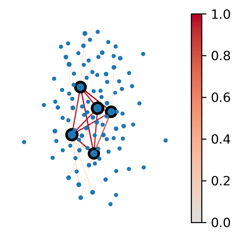
(a) Planted Clique

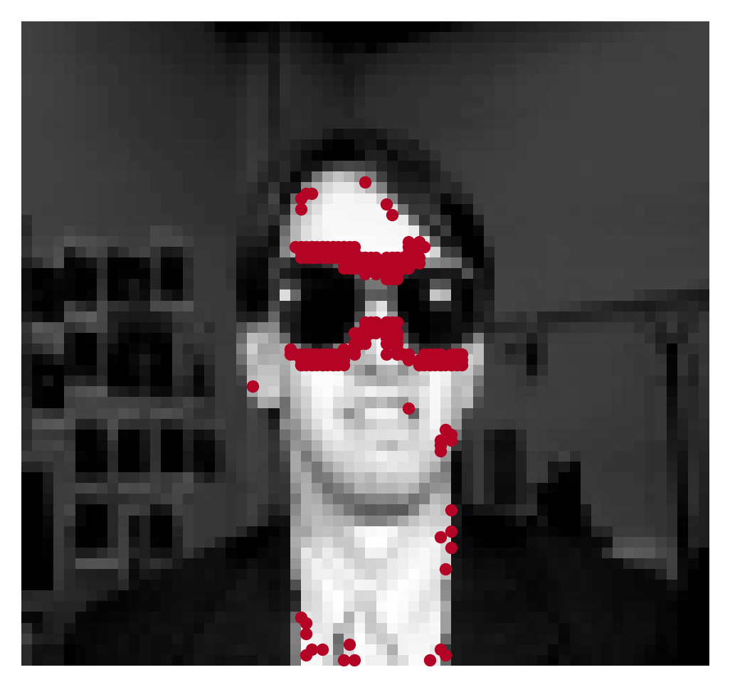
(b) Sunglasses - EASY

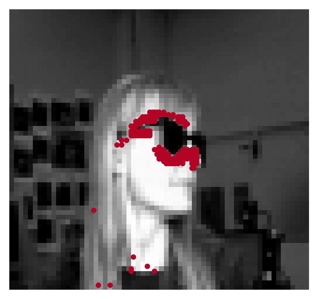
(c) Sunglasses - HARD

Figure 1: Explanations generated by our approach (RAGE) in two case studies: Planted Clique (graphs with and without cliques) and Sunglasses (headshots with and without sunglasses). RAGE explanations identify edges in the clique and in the region around the sunglasses for both difficulties. For Planted Clique (a), the heatmap and sizes show node and edge influences, and the nodes with a thick border are members of the planted clique. For Sunglasses (b-c), the red dots show the influential pixel connections to the detection. We will discuss these case studies in more detail later.

A critical problem in machine learning on graphs is understanding predictions made by graph-based models in high-stakes applications. This has motivated the study of graph explainers, which aim to identify subgraphs that are both compact and correlated with model decisions. However, there is no consensus on what constitutes a good explanation—i.e. correlation metric. Recent papers [1, 2, 3] have proposed different alternative notions of explainability that do not take the user into consideration and instead are validated using examples. On the other hand, other approaches have applied labeled explanations to learn an explainer directly from data [4]. However, such labeled explanations are hardly available.

Explainers can be divided into post-hoc and ante-hoc (or intrinsic) [5]. Post-hoc explainers treat the prediction model as a black box and learn explanations by modifying the input of a pre-trained model [6]. On the other hand, ante-hoc explainers learn explanations as part of the model. The key advantage of post-hoc explainers is flexibility since they make no assumption about the prediction model to be explained or the training algorithm applied to learn the model. However, these explanations have two major limitations: (1) they are not sufficiently informative to enable the user to reproduce the behavior of the model, and (2) they are often based on a model that was trained without taking explainability into account.

The first limitation is based on the intuitive assumption that a good explanation should enable the user to approximately reproduce the decisions of the model for new input. That is simply because the predictions will often depend on parts of the input that are not part of the explanation. The second limitation is based on the fact that for models with a large number of parameters, such as neural networks, there are likely multiple parameter settings that achieve similar values of the loss function. However, only some of such models might be explainable [7, 8]. While these limitations do not necessarily depend on a specific model, this paper addresses them in the context of Graph Neural Networks for graph-level tasks (classification and regression).

We propose RAGE—a novel ante-hoc explainer for graphs—that aims to find compact explanations while maximizing the graph classification/regression accuracy using bilevel optimization. Figure 2 compares the post-hoc and ante-hoc approaches in the context of graph classification. RAGE explanations are given as input to the GNN, which guarantees that no information outside of the explanation is used for prediction. This enables the user to select an appropriate trade-off between the compactness of the explanations and their discrimination power. We show that RAGE explanations are more robust to noise in the input graph than existing (post-hoc and ante-hoc) alternatives. Moreover, our explanations are learned jointly with the GNN, which enables RAGE to learn GNNs that are accurate and explainable. In fact, we show that RAGE’s explainability objective produces an inductive bias that often improves the accuracy of the learned GNN compared to the base model. We emphasize that while RAGE is an ante-hoc model, it is general enough to be applied to a broad class of GNNs.

Figure 1 shows examples of RAGE explanations in two case studies. In 1a, we show an explanation from a synthetic dataset (Planted Clique), where the goal is to classify whether the graph has a planted clique or not based on examples. As expected, the edge influences learned by RAGE match with the planted clique. In 1b, we show an explanation for a real dataset (Sunglasses) with graphs representing headshots (images), where the goal is to classify whether the person in the corresponding headshot is wearing sunglasses. We notice that edge influences highlight pixels around the sunglasses. We provide a detailed case study using these two datasets in Section 3.5, including a comparison against state-of-the-art post-hoc and ante-hoc explainers. We also evaluate our approach quantitatively in terms of accuracy, reproducibility, and robustness. Our results show that RAGE often outperforms several baselines. Our main contributions can be summarized as follows:

• We highlight and empirically demonstrate two important limitations of post-hoc graph explainers. They do not provide enough information to enable reproducing the behavior of the predictor and are based on fixed models that might be accurate but not explainable.

• We propose RAGE, a novel GNN and flexible explainer for graph classification and regression tasks. RAGE applies bilevel optimization, learning GNNs in the inner problem and an edge influence function in the outer loop. Our approach is flexible enough to be applied to a broad class of GNNs.

• We compare RAGE against state-of-the-art graph classification and GNN explainer baselines using six datasets—including five real-world ones. RAGE not only outperforms the baselines in terms of accuracy in most settings but also generates explanations that are faithful, robust, and enable reproducing the behavior of the predictor. We also provide additional case studies showing that our method improves interpretability by highlighting essential parts of the input data.

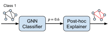
(a) Post-hoc Models

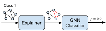
(b) Ante-hoc Models

Figure 2: (a) Post-hoc models generate explanations for a pre-trained GNN classifier using its predictions. (b) Ante-hoc models, as our approach, learn GNNs and explanations jointly. This enables ante-hoc models to identify GNNs that are both explainable and accurate.

2 Methodology

2.1 Problem Formulation

We formulate our problem as a supervised graph classification (or regression). Given a graph set $\mathcal{G}=\{G_{1},G_{2},\dots,G_{n}\}$ and continuous or discrete labels $\mathcal{Y}=\{y_{1},y_{2},\dots,y_{n}\}$ for each graph respectively, our goal is to learn a function $\hat{f}:\mathcal{G}\to\mathcal{Y}$ that approximates the labels of unseen graphs.

Figure 3: Illustration of an edge-based ante-hoc explainer that uses bilevel optimization. Explainer generates an explanation graph from the input graph by assigning an influence value to each edge. Edge influences are incorporated to edge weights on the explanation graph, the input of GNN Classifier. The inner problem optimizes GNN Classifier with $T$ iterations, while the outer problem updates Explainer using gradients from inner iterations. The dotted edges in the explanation graph show that they do not influence the classification, while others have different degrees of influence.

2.2 RAGE: Robust Ante-hoc Graph Explainer

We introduce RAGE, an ante-hoc explainer that generates robust explanations using bilevel optimization. RAGE performs compact and discriminative subgraph learning as part of the GNN training that optimizes the prediction of class labels in graph classification or regression tasks.

RAGE is based on a general scheme for an edge-based approach for learning ante-hoc explanations using bilevel optimization, as illustrated in Figure 3. The explainer will assign an influence value to each edge, which will be incorporated into the original graph. The GNN classifier is trained with this new graph over $T$ inner iterations. Gradients from inner iterations are kept to update the explainer in the outer loop. The outer iterations minimize a loss function that induces explanations to be compact (sparse) and discriminative (accurate). We will now describe our approach (RAGE) in more detail.

2.2.1 Explainer - Subgraph Learning

RAGE is an edge-based subgraph learner. It learns edge representations from the node representations/features. Surprisingly, most edge-based explainers for undirected graphs are not permutation invariant when calculating edge representations (e.g., PGExplainer [2] concatenates node representations based on their index order). Shuffling nodes could change their performance drastically since the edge representations would differ. We calculate permutation invariant edge representations $h_{ij}$ given two node representations $h_{i}$ and $h_{j}$ as follows: $h_{ij}=[\textbf{max}(h_{i},h_{j});\textbf{min}(h_{i},h_{j})]$, where max and min are pairwise for each dimension and $[\cdot;\cdot]$ is the concatenation operator.

Edge influences are learned via an MLP with sigmoid activation based on edge representations: $z_{ij}=MLP(h_{ij})$. This generates an edge influence matrix $Z\!\in\![0,1]^{nxn}$. We denote our explainer function as $g_{\Phi}$ with trainable parameters $\Phi$.

2.2.2 Influence-weighted Graph Neural Networks

Any GNN architecture can be made sensitive to edge influences $Z$ via a transformation of the adjacency matrix of the input graphs. As our model does not rely on a specific architecture, we will refer to it generically as $GNN(A,X)$, where $A$ and $X$ are the adjacency and attribute matrices, respectively. We rescale the adjacency matrix with edge influences $Z$ as follows: $A_{Z}=Z\odot A$.

The GNN treats $A_{Z}$ in the same way as the original matrix: $H=GNN(A_{Z},X)$

We generate a graph representation $h$ from the node representation matrix $H$ via a max pooling operator. The graph representation $h$ is then given as input to a classifier that will predict graph labels $y$. Here, we use an MLP as our classifier.

2.2.3 Bilevel Optimization

In order to perform both GNN training and estimate the influence of edges jointly, we formulate graph classification as a bilevel optimization problem. In the inner problem (Equation 2), we learn the GNN parameters $\theta^{*}\in\mathbb{R}^{h}$ given edges influences $Z^{*}\in[0,1]^{nxn}$ based on a training loss $\ell^{tr}$ and training data $(D^{tr},y^{tr})$. We use the symbol $C$ to refer to any GNN architecture. In the outer problem (Equation 1), we learn edge influences $Z^{*}$ by minimizing the loss $\ell^{sup}$ using support data $(D^{sup},y^{sup})$. The loss functions for the inner and outer problem, $f_{Z^{*}}$ and $F$, also apply regularization functions, $\Theta_{inner}$ and $\Theta_{outer}$, respectively.

$$Z^{*}=\operatorname*{arg\,min}_{Z}F(\theta^{*},Z)=\ell^{sup}(C(\theta^{*},Z,D^{sup}),y^{sup})+\Theta_{outer}$$ (1)

$$\theta^{*}=\operatorname*{arg\,min}_{\theta}f_{Z^{*}}(\theta)=\ell^{tr}(C(\theta,Z^{*},D^{tr}),y^{tr})+\Theta_{inner}$$ (2)

RAGE can be understood through the lens of meta-learning. The outer problem performs meta-training and edge influences are learned by a meta-learner based on support data. The inner problem solves multiple tasks representing different training splits sharing the same influence weights.

At this point, it is crucial to justify the use of bilevel optimization to compute edge influences $Z$. A simpler alternative would be computing influences as edge attention weights using standard gradient-based algorithms (i.e., single-level). However, we argue that bilevel optimization is a more robust approach to our problem. More specifically, we decouple the learning of edge influences from the GNN parameters and share the same edge influences in multiple training splits. Consequently, these influences are more likely to generalize to unseen data. We validate this hypothesis empirically using different datasets in our experiments (Supp. D.1).

2.2.4 Loss Functions

RAGE loss functions have two main terms: a prediction loss and a regularization term. As prediction losses, we apply cross-entropy or mean-square-error, depending on whether the problem is classification or regression. The regularization for the inner problem $\Theta_{inner}$ is a standard $L_{2}$ penalty over the GNN weights $\theta$. For the outer problem $\Theta_{outer}$, we also apply an $L_{1}$ penalty to enforce the sparsity of $Z$. Finally, we also add an $L_{2}$ penalty on the weights of $g_{\Phi}$.

2.3 Bilevel Optimization Training

The main steps performed by our model (RAGE) are given in Algorithm 1. For each outer iteration (lines 1-14), we split the training data into two sets—training and support—(line 2). First, we use training data to calculate $Z^{tr}$, which is used for $GNN$ training in the inner loop (lines 5-10). Then, we apply the gradients from the inner problem to optimize the outer problem using support data (lines 11-13). Note that we reinitialize $GNN$ and $MLP$ parameters (line 4) before starting inner iterations to remove undesirable information [9] and improve data generalization [10]. We further discuss the significance and the impact of this operation in Supp D.2. The main output of our algorithm is the explainer $g_{\Phi_{\kappa}}$. Moreover, the last trained $GNN_{\theta_{T}}$ can also be used for the classification of unseen data, or a new GNN can be trained based on $Z$. In both cases, the GNN will be trained with the same input graphs, which guarantees the behavior of the model $GNN_{\theta_{T}}$ can be reproduced using explanations from $g_{\Phi_{\kappa}}$.

For gradient calculation, we follow the gradient-based approach described in [11]. The critical challenge of training our model is how to compute gradients of our outer objective with respect to edge influences $Z$. By the chain rule, such gradients depend on the gradient of the classification/regression training loss with respect to $Z$. We will, again, use the connection between RAGE and meta-learning to describe the training algorithm.

2.3.1 Training (Inner Loop)

At inner loop iterations, we keep gradients while optimizing model parameters $\theta$.

$$\theta_{t+1}=inner\text{-}opt_{t}\left(\theta_{t},\nabla_{\theta_{t}}\ell^{tr}(\theta_{t},Z_{\tau})\right)$$

After T iterations, we compute $\theta^{*}$, which is a function of $\theta_{1},\dots,\theta_{T}$ and $Z_{\tau}$, where $\tau$ is the number of iterations for meta-training. Here, $inner\text{-}opt_{t}$ is the inner optimization process that updates $\theta_{t}$ at step $t$. If we use SGD as an optimizer, $inner\text{-}opt_{t}$ will be written as follows with a learning rate $\eta$:

$$inner\text{-}opt_{t}\left(\theta_{t},\nabla_{\theta_{t}}\ell^{tr}(\theta_{t},Z_{\tau})\right)\coloneqq\theta_{t}-\eta\cdot\nabla_{\theta_{t}}\ell^{tr}(\theta_{t},Z_{\tau})$$

2.3.2 Meta-training (Outer Loop)

After $T$ inner iterations, the gradient trajectory saved to $\theta^{*}$ will be used to optimize $\Phi$. We denote $outer\text{-}opt_{\tau}$ as outer optimization that updates $\Phi_{\tau}$ at step $\tau$. The meta-training step is written as:

$$\Phi_{\tau+1}= \ outer\text{-}opt_{\tau}\left(\Phi_{\tau},\nabla_{\Phi_{\tau}}\ell^{sup}(\theta^{*})\right)$$

$$= \ outer\text{-}opt_{\tau}\left(\Phi_{\tau},\nabla_{\Phi_{\tau}}\ell^{sup}(inner\text{-}opt_{T}(\theta_{T},\nabla_{\theta_{T}}\ell^{tr}(\theta_{T},z_{\tau})))\right)$$

Algorithm 1 RAGE

0:  Graphs $A_{1:n}$, node attributes $X_{1:n}$, labels $y_{1:n}$, explainer $g_{\Phi_{0}}$, outer/inner loops $\kappa$ and $T$

0:  Trained $g_{\Phi_{\kappa}}$

1:  for $\tau\in[0,\kappa-1]$ do

2:     $A^{tr},A^{sup},X^{tr},X^{sup},y^{tr},y^{sup}\leftarrow\text{split}(A_{1:n},X_{1:n},y_{1:n})$

3:     $Z^{tr}\leftarrow g_{\Phi_{\tau}}(A^{tr},X^{tr})$

4:     (re)initialize $GNN_{\theta_{0}}$, $MLP_{\theta_{0}}$

5:     for $t\in[0,T-1]$ do

6:        $H^{tr}\leftarrow GNN_{\theta_{t}}(Z^{tr}\odot A^{tr},X^{tr})$

7:        $h^{tr}\leftarrow POOL_{max}(H^{tr})$

8:        $p^{tr}\leftarrow MLP_{\theta_{t}}(h^{tr})$

9:        $GNN_{\theta_{t+1}},MLP_{\theta_{t+1}}\leftarrow inner\text{-}opt\ \ f_{Z^{tr}}(p^{tr},y^{tr})$

10:     end for

11:     $Z^{sup}\leftarrow g_{\Phi_{\tau}}(A^{sup},X^{sup})$

12:     $p^{sup}\leftarrow MLP_{\theta_{T}}(POOL_{max}(GNN_{\theta_{T}}(Z^{sup}\odot A^{sup},X^{sup}))$

13:     $g_{\Phi_{\tau+1}}\leftarrow outer\text{-}opt\ \ F_{\theta_{T}}(p^{sup},y^{sup})$

14:  end for

15:  return   $g_{\Phi_{\kappa}}$

After each meta optimization step, we calculate edge influences $Z_{\tau+1}$ using $g_{\Phi_{\tau+1}}(.)$. Notice that our training algorithm is more computationally-intensive than training a simple GNN architecture. Therefore we set $T$ and $\kappa$ to small values. Thus, RAGE can also be efficiently applied at training and testing time compared to competing baselines (Supp F).

3 Experiments

We evaluate RAGE on several datasets, outperforming both post-hoc and ante-hoc explainers in terms of metrics, including discriminative power and robustness. A key advantage of our approach is being able to efficiently search for a GNN that is both explainable and accurate. Our case studies show the effectiveness of explanations generated by RAGE over the baselines. We provide more results and analysis on RAGE in the supplementary. Our implementation of RAGE is anonymously available at https://anonymous.4open.science/r/RAGE.

3.1 Experimental Settings

Datasets: We consider six graph classification (regression) datasets in our experiments. Table 1 shows the main statistics of them. More details are provided in the Supplementary.

Table 1: The statistics of the datasets.

	#Graphs	#Nodes	#Edges	#Features
Mutagenicity [12, 13]	4337	131488	133447	14
Proteins [14, 15]	1113	43471	81044	32
IMDB-B [16]	1000	19773	96531	136
Sunglasses [17]	624	2396160	9353760	1
Tree of Life [18]	1245	944888	5634922	64
Planted Clique	100	10000	49860	64

Baselines: We consider several classical baselines for graph classification and regression including GCN [19], GAT [20], GIN [21], and SortPool [22]). We also compare RAGE against ExpertPool [23], which learns attention weights for node pooling, and against state-of-the-art GNN-based methods such as DropGNN [24], GMT [25], GIB [26], ProtGNN [8], and those that apply graph structure learning including LDS-GNN [27] and VIB-GSL [28]. For methods that use node classification, we add an additional pooling layer to adapt to the graph classification setting. Finally, we consider inductive GNN explainers: PGExplainer [2], RCExplainer [3], TAGE [29]. We also used transductive explainers (GNNExplainer [1], SubgraphX [30], CF² [31]) for a Planted Clique case study (Supp. G).

Evaluation metrics: We compare the methods in terms of accuracy using AUC and AP for classification and also MSE and R² for regression. Moreover, we compare explanations in terms of faithfulness (Supp. B), stability [32], and reproducibility. Faithfulness measures how closely the classifier’s prediction aligns with the original graphs and their explanations. Stability (or robustness) quantifies the correlation between explanations generated for the original dataset and its noisy variants. Reproducibility assesses the accuracy of a GNN trained solely using the explanations as a dataset.

3.2 Graph Classification and Regression

Table 2 shows the graph classification (regression) results in terms of AUC (MSE) for RAGE and the baselines using five real-world and one synthetic datasets. RAGE outperforms the competing approaches in five datasets and has comparable results for IMDB-B. This indicates that our approach is able to identify subgraphs that are both compact and discriminative.

Each of its baselines has its own drawbacks and performs poorly on (at least) one dataset with the exception of ExpertPool, which has consistent performance across datasets. Still, RAGE outperforms ExpertPool for every dataset by $10.75\%$ on average and by up to $27.2\%$ on Tree of Life. Surprisingly, most baselines achieve poor results for the Sunglasses and Planted Clique datasets, with the best baselines achieving $93.68\%$ (ExpertPool) and $87.78\%$ (GIN) AUC, respectively. This is evidence that existing approaches, including GIB and ProtGNN, are not able to effectively identify compact discriminative subgraphs. We also notice that, comparatively, RAGE achieves the best results for real datasets with large graphs (Sunglasses and Tree of Life). Intuitively, these are datasets for which identifying discriminative subgraphs has the highest impact on performance. Additionally, baselines using graph structure learning have poor performance and are not able to scale to large datasets.

Table 2: Test scores for graph classification/regression. Best and second-best values are in bold and underlined for each dataset. RAGE achieves the best results on average, outperforming the baselines.

	Classification (AUC %)					Regression (MSE)
	Mutagenicity	Proteins	IMDB-B	Sunglasses	Planted Clique	Tree of Life
GCN [19]	$86.82\pm 0.39$	$82.71\pm 1.08$	$81.49\pm 1.16$	$79.66\pm 13.12$	$52.89\pm 15.87$	$0.222\pm 0.010$
GAT [20]	$86.05\pm 0.59$	$82.31\pm 1.70$	$80.66\pm 1.56$	$67.80\pm 15.37$	$51.78\pm 22.36$	$0.179\pm 0.018$
GIN [21]	$88.15\pm 0.37$	$82.65\pm 0.90$	$84.14\pm 1.20$	$55.25\pm 4.62$	$87.78\pm 12.36$	$0.751\pm 0.584$
ExpertPool [23]	$86.81\pm 0.47$	$81.33\pm 1.21$	$83.20\pm 0.48$	$93.68\pm 1.15$	$80.00\pm 19.12$	$0.010\pm 0.015$
SortPool [22]	$85.34\pm 0.64$	$82.76\pm 1.10$	$80.62\pm 1.43$	$93.26\pm 2.52$	$54.44\pm 26.97$	$0.098\pm 0.014$
DropGNN [24]	$84.86\pm 2.11$	$82.59\pm 4.13$	$\textbf{84.73}\pm\textbf{2.00}$	$54.74\pm 2.30$	$69.66\pm 12.70$	$2.690\pm 1.298$
GMT [25]	$86.06\pm 1.17$	$82.19\pm 3.13$	$80.82\pm 1.38$	$52.32\pm 1.21$	$56.39\pm 26.64$	$0.087\pm 0.004$
GIB [26]	$85.53\pm 0.99$	$82.71\pm 0.95$	$82.21\pm 2.04$	$61.30\pm 7.26$	$53.33\pm 16.33$	$0.305\pm 0.046$
ProtGNN [8]	$86.72\pm 0.62$	$81.21\pm 2.07$	$82.53\pm 2.37$	N/S	$57.78\pm 13.33$	N/A
LDS-GNN [27]	$86.12\pm 1.50$	$81.73\pm 1.32$	$81.12\pm 1.30$	OOM	$54.12\pm 15.32$	OOM
VIB-GSL [28]	$84.19\pm 1.10$	EG	$81.11\pm 1.21$	OOM	$54.44\pm 12.96$	OOM
RAGE	$\textbf{89.52}\pm\textbf{0.36}$	$\textbf{85.20}\pm\textbf{0.93}$	$84.16\pm 0.32$	$\textbf{99.36}\pm\textbf{0.44}$	$\textbf{97.78}\pm\textbf{4.44}$	$\textbf{0.073}\pm\textbf{0.007}$

• EG: Exploding Gradient    OOM: Out Of Memory    N/S: Not Scalable    N/A: Not Applicable

3.3 Reproducibility

Reproducibility measures how well explanations alone can predict class labels. It is a key property as it allows the user to correlate explanations and predictions without neglecting potentially relevant information from the input. In our evaluation, we vary the size of the explanations by thresholding edges based on their values. We then train a GNN using only the explanations and labels. We compare RAGE against post-hoc and ante-hoc explainers and the resulting accuracies are shown in Figure 4.

The results demonstrate that RAGE outperforms competing explainers in terms of reproducibility. Depending on the dataset, post-hoc and ante-hoc baselines may emerge as the second-best methods. TAGE (post-hoc), GIB (ante-hoc) and ProtGNN (ante-hoc), which aim to generalize the explanations through task-agnostic learning, bilevel optimization, and prototyping respectively, are among the most competitive baselines. This also highlights the importance of generalizability, which RAGE incorporates through meta-training and bilevel optimization. Two other post-hoc explainers, PGExplainer and RCExplainer, perform poorly. As expected, larger explanations lead to better reproducibility.

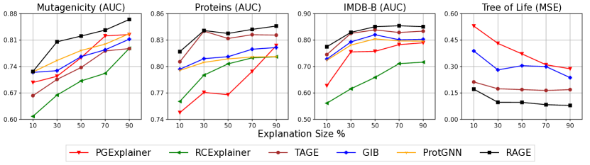
Figure 4: Reproducibility comparison between methods for different explanation sizes (in percentage) using four datasets. RAGE consistently outperforms the baselines across different sizes and datasets.

3.4 Robustness

Effective explanations should be robust to noise in the data. We evaluate the robustness of RAGE and the baselines using MutagenicityNoisyX—i.e. noisy versions of Mutagenicity with random edges (Supp. H.4 for details). We discuss results in terms of accuracy (Supp. C) and stability.

Stability: Figure 5 presents a comparison of explanations obtained from Mutagenicity dataset and its noisy variants, evaluated based on cosine distance and Pearson correlation. Our results demonstrate that RAGE outperforms other graph explainers in both metrics. Furthermore, TAGE and GIB are identified as competitive baselines, which is consistent with the reproducibility metric, while prototyping fails. These findings provide further evidence that RAGE’s approach for generalizability through meta-training and bilevel optimization contributes to the robustness of explanations. Furthermore, post-hoc explainers, PGExplainer and RCExplainer, are sentitive to noise, lacking stability.

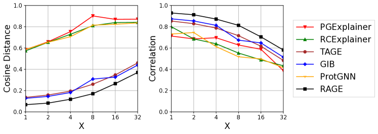
Figure 5: Cosine distance (lower is better) and Pearson correlation (higher is better) between explanations for Mutagenicity and MutagenicityNoisyX generated by RAGE and the baselines. RAGE is significantly more stable than the baselines, with GIB and TAGE as the best baselines.

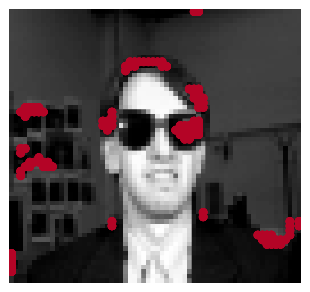
(a) PGExplainer

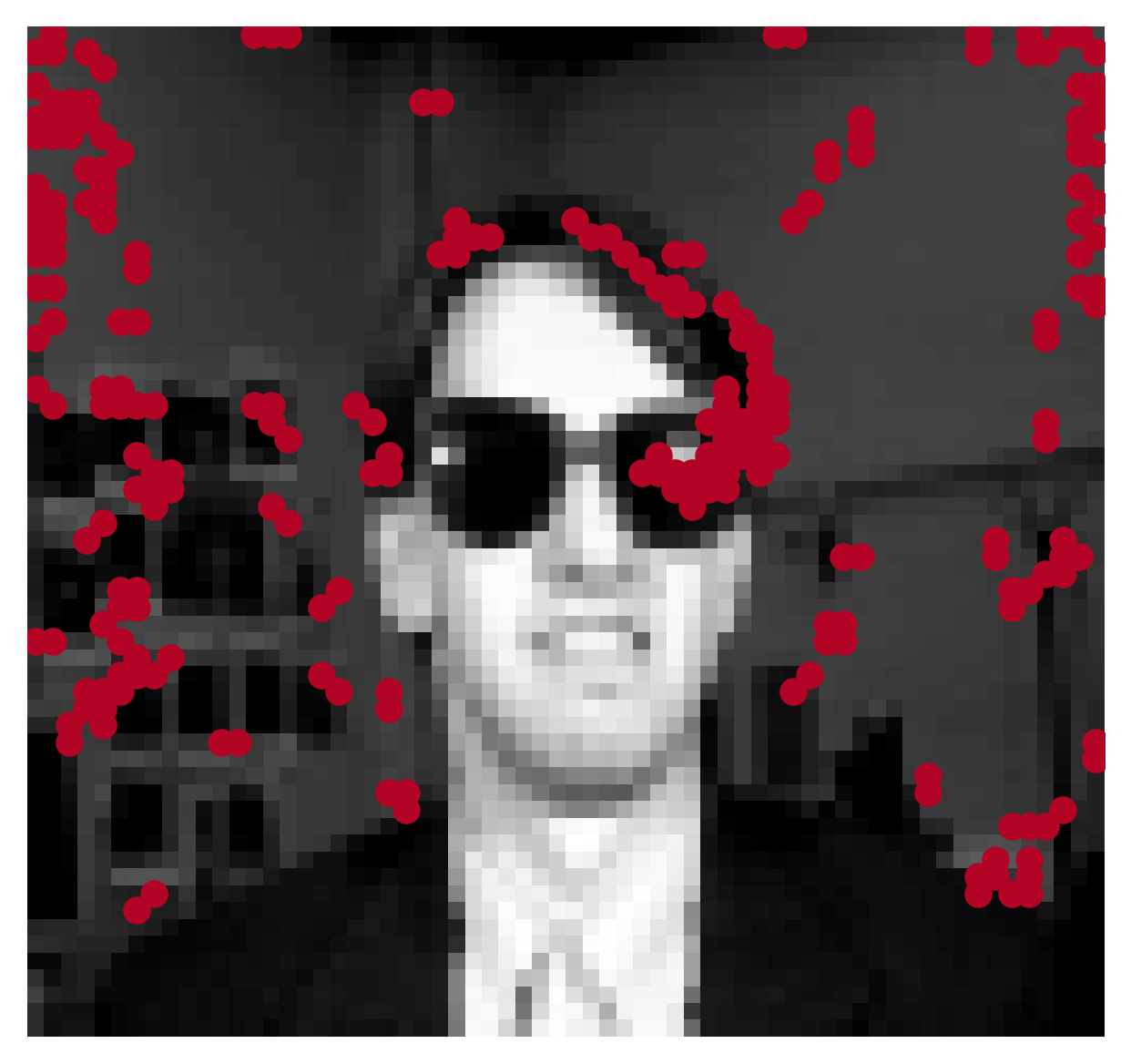
(b) TAGE

(c) GIB

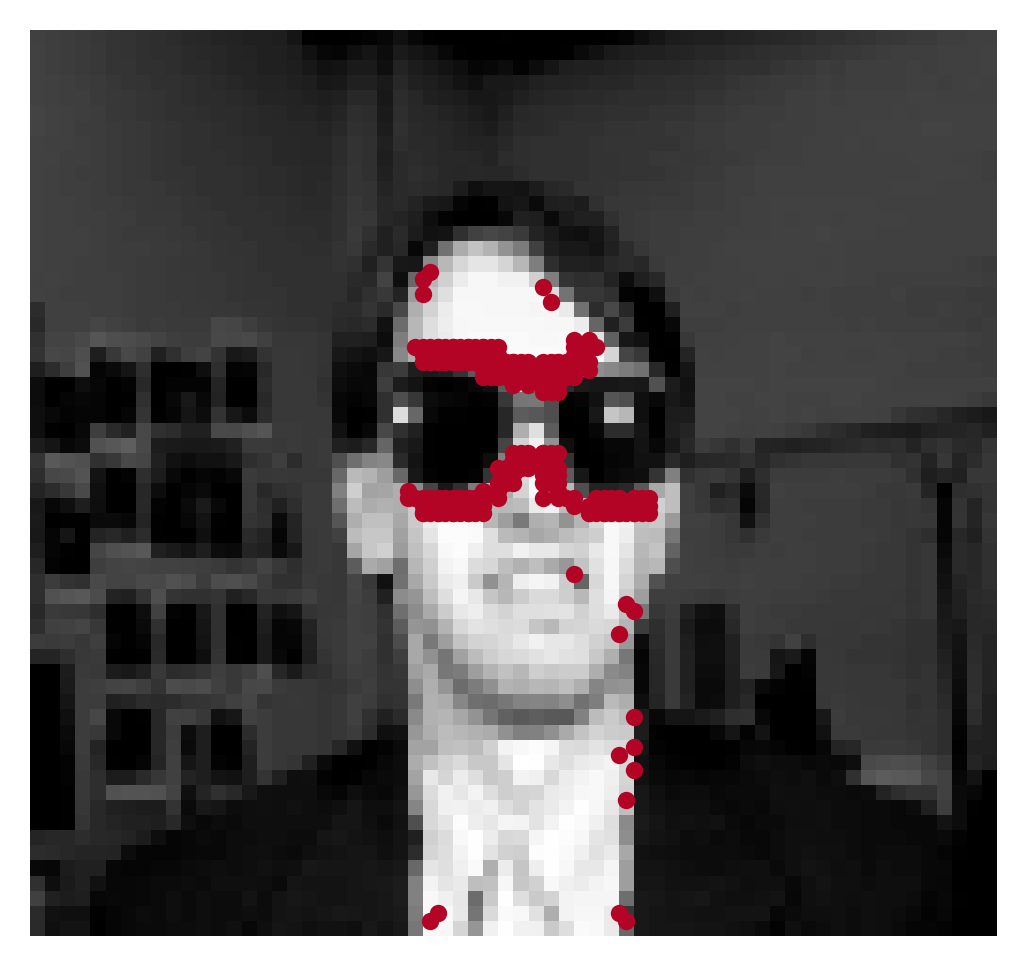
(d) RAGE

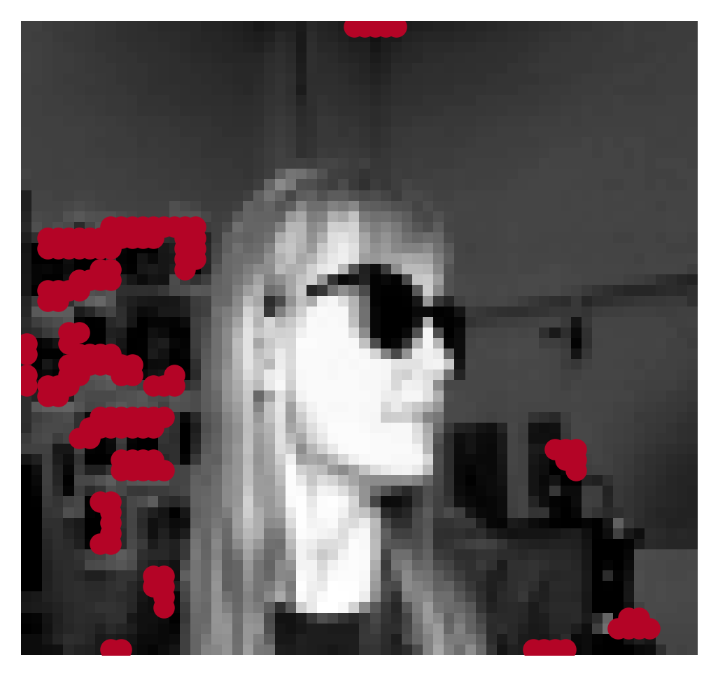
(e) PGExplainer

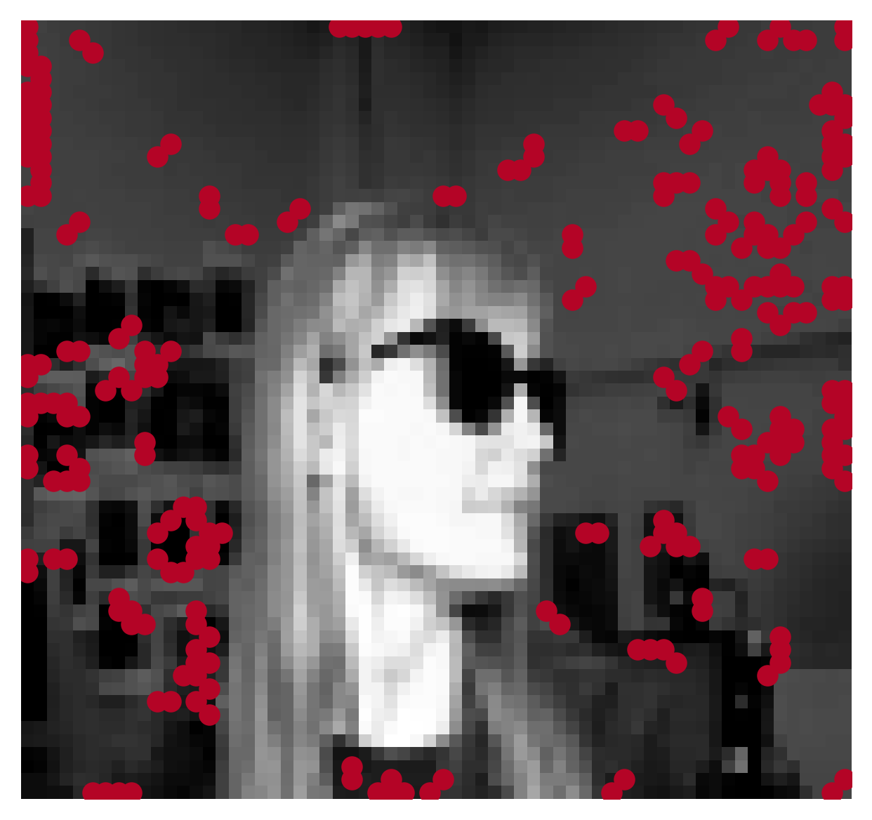
(f) TAGE

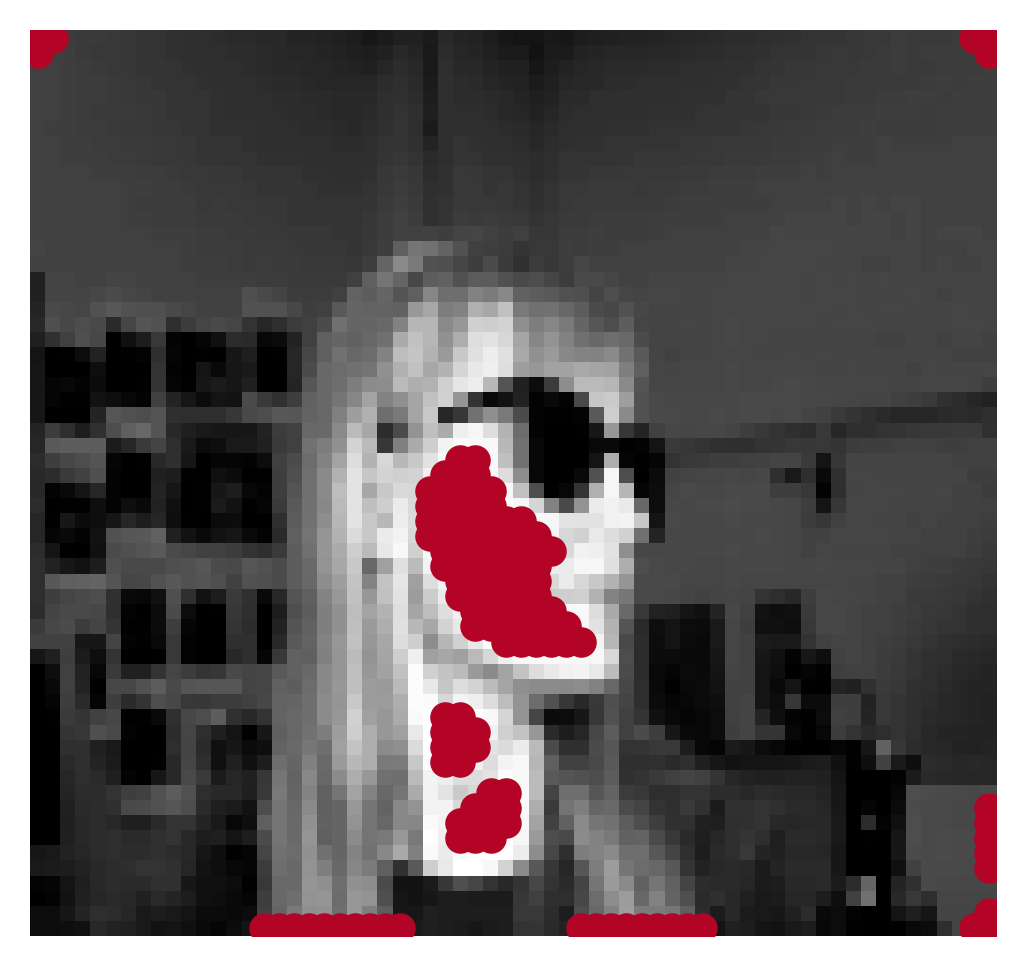
(g) GIB

(h) RAGE

Figure 6: Two examples with different levels of difficulty due to poses from the Sunglasses dataset. RAGE is able to detect the edges between the sunglasses and the human faces, which are the most relevant for the prediction task (i.e., whether the human is wearing sunglasses) for both examples.

3.5 Case Study

We present a case study from Sunglasses (an extra case study for the Planted Clique in the Supplementary G) that showcases the explanations generated by RAGE and compares them to those generated by post-hoc and ante-hoc baselines at Figure 6. Sunglasses contains ground truth explanations that are intuitive. It is worth noting that the examples in the dataset have different levels of difficulty due to variations in the poses of the individuals in the pictures (bottom is harder).

RAGE successfully detects edges at the border between the sunglasses and the faces of the humans in both pictures, which are the edges most relevant for the prediction task - i.e. detecting whether the human is wearing sunglasses. These highlighted edges are the most influential ones for the learned GNN, which is consistent with the high accuracy results presented in Table 2. However, PGExplainer and TAGE identify only one of the glasses as an explanation for the easier pose (Figure 6a and 6b). PGExplainer also signifies other dark pixels in the image whereas TAGE explanations are hard to interpret. For the more challenging pose, PGExplainer and TAGE miss the sunglasses completely. Meanwhile, GIB explanations do not match the sunglasses in either example, which explains their poor performance on this dataset (see Table 2). Unfortunately, we were unable to apply RCExplainer and ProtGNN to this dataset due to an out-of-memory error and scalability issues, respectively.

4 Related Work

Graph classification with GNNs: Graph Neural Networks (GNNs) have gained prominence in graph classification due to their ability to learn features directly from data [19, 20, 33, 21]. GNN-based graph classifiers aggregate node-level representations via pooling operators to represent the entire graph. The design of effective graph pooling operators is key for effective graph classification [34, 22, 23, 35]. However, simple pooling operators that disregard the graph structure, such as mean and max, remain popular and have been shown to have comparable performance to more sophisticated alternatives [36]. Recently, [25] proposed a multi-head attention pooling layer to capture structural dependencies between nodes. In this paper, we focus on graph classification and regression tasks. We show that our approach increases the discriminative power of GNNs for classification by learning effective explanations, outperforming state-of-the-art alternatives from the literature [21, 25, 24].

Explainability of GNNs: Explainability has become a key requirement for the application of machine learning in many settings (e.g., healthcare, court decisions) [37]. Several post-hoc explainers have been proposed for explaining Graph Neural Networks’ predictions using subgraphs [1, 2, 30, 3, 31, 29]. GNNExplainer [1] applies a mean-field approximation to identify subgraphs that maximize the mutual information with GNN predictions. PGExplainer [2] applies a similar objective, but samples subgraphs using the reparametrization trick. RCExplainer [3] identifies decision regions based on graph embeddings that generate a subgraph explanation such that removing it changes the prediction of the remaining graph (i.e., counterfactual). While post-hoc explainers treat a trained GNN as a black box —i.e., it only relies on predictions made by the GNN—ante-hoc explainers are model-dependent. GIB [26] applies the bottleneck principle and bilevel optimization to learn subgraphs relevant for classification but different from the corresponding input graph. ProtGNN [8] learns prototypes (interpretable subgraphs) for each class and makes predictions by matching input graphs and class prototypes. Bilevel optimization and prototypes help in generalizability of explanations. Recently, TAGE [29] proposes task-agnostic post-hoc graph explanations which also makes the explanations generalizable compared to existing post-hoc explainers. However, it is still outperformed by our ante-hoc explainer, which applies meta-training and bilevel optimization, in terms of different metrics. Our experiments show that RAGE explanations are more meaningful, faithful, and robust than alternatives and can reproduce the model behavior better than existing post-hoc and ante-hoc explainers.

Bilevel optimization: Bilevel optimization is a class of optimization problems where two objective functions are nested within each other [38]. Although the problem is known to be NP-hard, recent algorithms have enabled the solution of large-scale problems in machine learning, such as automatic hyperparameter optimization and meta-learning [39]. Bilevel optimization has recently also been applied to graph problems, including graph meta-learning [40] and transductive graph sparsification scheme [41]. Like RAGE, GIB [26] also applies bilevel optimization to identify discriminative subgraphs inductively. However, we show that our approach consistently outperforms GIB in terms of discriminative power, reproducibility, and robustness.

Graph structure learning: Graph structure learning (GSL) aims to enhance (e.g., complete, de-noise) graph information to improve the performance of downstream tasks [42]. LDS-GNN [27] applies bilevel optimization to learn the graph structure that optimizes node classification. VIB-GSL [28] advances GIB [26] by applying a variational information bottleneck on the entire graph instead of only edges. We notice that GSL mainly focuses on learning the entire graph, whereas we only sparsify the graph, which reduces the search space and is more interpretable than possibly adding new edges. Furthermore, learning the entire graph is not scalable in large graph settings.

5 Conclusion

We investigate the problem of generating explanations for GNN-based graph-level tasks (classification and regression) and propose RAGE, a novel ante-hoc GNN explainer based on bilevel optimization. RAGE inductively learns compact and accurate explanations by optimizing the GNN and explanations jointly. Moreover, different from several baselines, RAGE explanations do not omit any information used by the model, thus enabling the model behavior to be reproduced based on the explanations. We compared RAGE against state-of-the-art graph classification methods and GNN explainers using synthetic and real datasets. The results show that RAGE often outperforms the baselines in terms of multiple evaluation metrics, including accuracy and robustness to noise. Furthermore, our two case studies illustrate the superiority of RAGE over state-of-the-art post-hoc and ante-hoc explainers.

Table 3: AP and $R^{2}$ scores for graph classification/regression. Best and second-best values are in bold and underlined for each dataset. RAGE outperforms the competing baselines on all datasets except IMDB-B to GIN, which performs poorly in larger datasets: Sunglasses and Tree of Life.

	Classification (AP)					Regression ($R^{2}$)
	Mutagenicity	Proteins	IMDB-B	Sunglasses	Planted Clique	Tree of Life
GCN [19]	$85.71\pm 0.53$	$81.37\pm 1.38$	$81.86\pm 1.62$	$79.48\pm 13.21$	$51.41\pm 3.60$	$52.90\pm 2.06$
GAT [20]	$84.84\pm 0.91$	$81.71\pm 1.97$	$80.49\pm 1.93$	$69.15\pm 14.34$	$51.06\pm 5.11$	$62.00\pm 3.76$
GIN [21]	$87.36\pm 0.47$	$80.56\pm 1.95$	$\textbf{84.69}\pm\textbf{1.34}$	$57.84\pm 4.29$	$86.92\pm 11.42$	$<0$
ExpertPool [23]	$85.23\pm 1.11$	$80.60\pm 1.41$	$83.78\pm 0.52$	$93.58\pm 1.38$	$73.83\pm 14.96$	$78.87\pm 3.20$
SortPool [22]	$84.43\pm 0.61$	$81.79\pm 1.51$	$81.47\pm 1.38$	$93.36\pm 2.71$	$58.39\pm 7.33$	$79.32\pm 2.90$
DropGNN [24]	$86.17\pm 1.28$	$81.35\pm 2.97$	$83.75\pm 0.99$	$53.00\pm 3.42$	$70.83\pm 25.34$	$<0$
GMT [25]	$85.35\pm 1.09$	$80.19\pm 2.13$	$79.56\pm 1.14$	$51.32\pm 1.13$	$59.28\pm 7.94$	$82.22\pm 0.83$
GIB [26]	$85.92\pm 1.04$	$81.52\pm 0.98$	$83.36\pm 1.92$	$62.24\pm 6.75$	$57.22\pm 3.82$	$35.34\pm 9.66$
ProtGNN [8]	$85.54\pm 0.94$	$80.28\pm 2.14$	$83.29\pm 2.91$	N/S	$54.22\pm 2.69$	N/A
LDS-GNN [27]	$85.03\pm 1.20$	$81.96\pm 1.54$	$81.01\pm 1.84$	OOM	$56.67\pm 9.57$	OOM
VIB-GSL [28]	$83.20\pm 1.74$	EG	$82.36\pm 1.18$	OOM	$56.12\pm 6.80$	OOM
RAGE	$\textbf{88.46}\pm\textbf{0.79}$	$\textbf{85.26}\pm\textbf{1.17}$	$84.00\pm 1.14$	$\textbf{99.36}\pm\textbf{0.43}$	$\textbf{94.89}\pm\textbf{10.22}$	$\textbf{84.61}\pm\textbf{1.45}$

• EG: Exploding Gradient    OOM: Out Of Memory    N/S: Not Scalable    N/A: Not Applicable    $<0$: No Relationship

Appendix A Further Evaluation of Graph Classification and Regression

Table 3 investigates graph classification and regression further by considering other metrics: Average Precision (AP) for graph classification and $R^{2}$ score for regression. RAGE still outperforms the competing baselines for almost all datasets. AP and R² results are similar quite similar to Table 2. The only noticeable difference is that GIN is now the best-performing method for IMDB-B. However, it fails in the regression task (Tree of Life) and cannot generate distinctive graph embeddings. We additionally calculate Accuracy measurement, and RAGE has 84.37% accuracy on average over datasets, 9% better than the best baseline ExpertPool (77.22%).

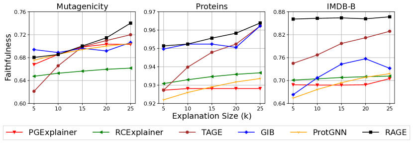
Figure 7: Faithfulness with respect to sparsity based on probability of sufficiency of RAGE and graph explainer baselines. RAGE generates comparable or more faithful explanations than the competing baselines.

Appendix B Evaluation of Explanations: Faithfulness with respect to Sparsity

We assessed the faithfulness of explanations produced by RAGE, as well as competing post-hoc and ante-hoc graph explainer baselines. For each method, we selected the top $k$ edges from the graph as its explanation, and we measured faithfulness using the probability of sufficiency metric [31].

Figure 7 demonstrates that RAGE generates explanations that are as faithful as, or more faithful than, the explanations produced by the competing baselines, across different sizes ($k$) of explanations for three graph classification datasets. The results for faithfulness are also correlated with the reproducibility and stability results, with the best-performing baselines being TAGE (post-hoc), GIB (ante-hoc) in most cases. This provides further evidence of the importance of generalizability for explanation performance. Notably, even with the smallest explanation size, RAGE exhibits superior faithfulness compared to the best-performing post-hoc explanation method, TAGE.

Appendix C Further Evaluation of Robustness: Accuracy under Noise

Figure 8 shows the test performance of RAGE and the baselines for different amounts of noise $X$. RAGE consistently outperforms the baselines in all settings. More interestingly, the gap between RAGE and the baselines increases with the amount of noise ($X$) in the dataset. Graph structure learning makes LDS-GNN robust to noise compared to other baselines, nevertheless, it is still outperformed by RAGE.

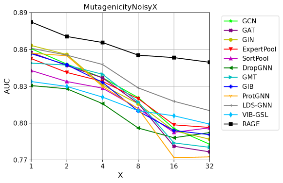
Figure 8: Test scores for graph classification (AUC) for noisy versions of the Mutagenicity dataset. RAGE outperforms all baselines, and the gap also increases with the amount of noise in the dataset.

Appendix D Further Ablation Study

Table 4: Test scores (AUC and MSE) of RAGE and its single-level variant RAGE-single for all datasets. RAGE outperforms RAGE-single in all datasets. Nevertheless, RAGE-single still has consistent performance across datasets and comparable results to graph classification baselines.

	RAGE	RAGE-single
Mutagenicity	$89.52\pm 0.36$	$88.79\pm 0.82$
MutagenicityNoisy1	$88.24\pm 0.67$	$86.05\pm 0.86$
MutagenicityNoisy2	$87.06\pm 0.46$	$85.87\pm 1.34$
MutagenicityNoisy4	$86.57\pm 0.63$	$84.55\pm 1.36$
MutagenicityNoisy8	$85.34\pm 0.16$	$82.68\pm 0.87$
MutagenicityNoisy16	$84.54\pm 0.65$	$80.21\pm 1.59$
MutagenicityNoisy32	$83.96\pm 0.95$	$79.16\pm 1.08$
Proteins	$85.20\pm 0.93$	$84.05\pm 1.26$
IMDB-B	$84.16\pm 0.32$	$82.26\pm 1.42$
Sunglasses	$99.36\pm 0.44$	$95.23\pm 1.51$
Planted Clique	$97.78\pm 4.44$	$86.67\pm 12.96$
Tree of Life (MSE)	$0.0725\pm 0.0068$	$0.1002\pm 0.0101$

D.1 Single-level Optimization

We create a single-level version of RAGE (RAGE-single) to test the effectiveness of our bilevel optimization scheme. More specifically, RAGE-single optimizes the explainer and GNN classifier parts in an end-to-end fashion with a single loss function. Table 4 shows that RAGE consistently outperforms RAGE-single. The performance gap is more prominent for large (e.g., Tree of Life) and noisy datasets. This is expected since large and noisy datasets are more prone to overfitting. Nevertheless, RAGE-single still achieves results comparable to graph classification baselines. Furthermore, to show the significance of our results, we conducted a paired t-test and obtained p-values that demonstrate the statistical significance of our findings for all datasets. Notably, all p-values were found to be strictly less than 0.005.

Table 5: Test scores (AUC and MSE) of RAGE and its without reinitilization variant RAGE-keep for all datasets. RAGE outperforms RAGE-keep in all datasets except Planted Clique which has the same performance. The usefulness of reinitilization is more obvious in larger datasets.

	RAGE	RAGE-keep
Mutagenicity	$89.52\pm 0.36$	$85.76\pm 0.77$
Proteins	$85.20\pm 0.93$	$84.47\pm 0.68$
IMDB-B	$84.16\pm 0.32$	$83.46\pm 1.20$
Sunglasses	$99.36\pm 0.44$	$70.66\pm 6.88$
Planted Clique	$97.78\pm 4.44$	$97.78\pm 4.44$
Tree of Life (MSE)	$0.0725\pm 0.0068$	$0.0912\pm 0.0056$

D.2 Keeping Base Model

RAGE incorporates reinitialization of the base GNN parameters before each inner loop iteration to eliminate unnecessary training trajectory from previously found explanations. This technique is known to reinforce effective features that may work under different conditions, as suggested by Zhou et al. [9]. Since the objective of RAGE is to combine sparsity and accuracy, there is no incentive to retain subgraphs that are unlikely to be used by the GNNs learned during the inner loop for making predictions. Therefore, restarting the entire GNN process after each iteration of RAGE is an effective approach to obtain a good representation of the subgraphs that will be applied by any accurate GNN trained using our method. Additionally, reinitializing neural network weights has been found to improve generalization on data, as discussed by Alabdulmohsin et al. [10].

To demonstrate the effect of reinitialization, we created a version of RAGE (RAGE-keep) without reinitializing the base $GNN$. The results of Table 5 indicate that reinitialization significantly improved the classifier quality. Notably, for larger datasets like Sunglasses, the difference was more pronounced. Furthermore, we conducted a paired t-test to show the statistical significance of our findings for all datasets. The p-values for all datasets were found to be strictly less than 0.01, except Planted Clique, which has the same performance.

Table 6: AUC and MSE test scores of GIB and its variant GIB-edge for all datasets. GIB-edge outperforms GIB-node consistently for all datasets.

	GIB-node	GIB-edge
Mutagenicity	$85.53\pm 0.99$	$86.24\pm 0.64$
MutagenicityNoisy1	$85.66\pm 0.44$	$85.93\pm 0.37$
MutagenicityNoisy2	$84.75\pm 0.13$	$85.57\pm 0.45$
MutagenicityNoisy4	$83.32\pm 0.63$	$83.68\pm 0.65$
MutagenicityNoisy8	$81.73\pm 0.75$	$81.01\pm 0.80$
MutagenicityNoisy16	$79.40\pm 0.64$	$80.28\pm 0.31$
MutagenicityNoisy32	$79.06\pm 0.54$	$79.25\pm 0.54$
Proteins	$82.71\pm 0.95$	$84.33+-0.90$
IMDB-B	$82.21\pm 2.04$	$83.10\pm 1.86$
Sunglasses	$61.30\pm 7.26$	$71.55\pm 14.23$
Planted Clique	$53.33\pm 16.33$	$66.67\pm 15.71$
Tree of Life (MSE)	$0.3047\pm 0.0455$	$0.1266\pm 0.0113$

D.3 Edge Influence for GIB

We claim that learning edge influence and using them during GNN aggregations is better than learning node weights during pooling. Originally, GIB [26] learned node weights and used them during the pooling operator. From the learned node weights, we calculate edge weights as average of node weights for each existed edge. Later, we retrain GNN using these edge weights with a max pooling operator. Table 6 shows that using edge weights is more effective than using node weights consistently for all datasets. Note that compared to the results from Table 2, GIB-edge still is outperformed by RAGE for all datasets. However, it competes better with other graph classification methods.

Table 7: AUC scores for graph classification and regression tasks using different GNN Encoder for RAGE. The results are consistent with different encoders. RAGE-GIN on IMDB-B has the most attention-getting result.

	RAGE-GCN	RAGE-GAT	RAGE-GIN
Mutagenicity	89.52	88.80	89.46
MutagenicityNoisy1	88.24	88.60	89.19
MutagenicityNoisy2	87.06	86.42	87.01
MutagenicityNoisy4	86.57	86.57	86.31
MutagenicityNoisy8	85.54	85.93	84.84
MutagenicityNoisy16	85.34	83.88	84.66
MutagenicityNoisy32	84.96	84.24	85.02
Proteins	85.20	84.05	84.94
IMDB-B	84.16	83.76	86.14
Sunglasses	99.26	95.95	90.08
Planted Clique	97.78	95.33	100.0
Tree of Life (MSE)	0.0725	0.0881	0.1217

D.4 Different GNN Encoder

RAGE works with any GNN encoder. In the main text, we provide the results from RAGE-GCN in Table 2. To show RAGE’s flexibility to pair with other GNN encoders, we ran experiments using GAT and GIN instead of the GCN encoder, and denote RAGE-GAT and RAGE-GIN, respectively. Table 7 shows that the results are consistent with Table 2. We also notice that even though there is a performance difference between original GCN, GAT, and GIN algorithms, RAGE variants do not differ much. However, the most interesting result is RAGE-GIN on the IMDB-B dataset. RAGE-GIN also outperforms the best baseline, DropGNN, in Table 2. To make the comparison fair, we change the GNN encoder of DropGNN to GIN and rerun the experiments. RAGE-GIN ($86.14\%$) still outperforms DropGIN ($85.82\%$).

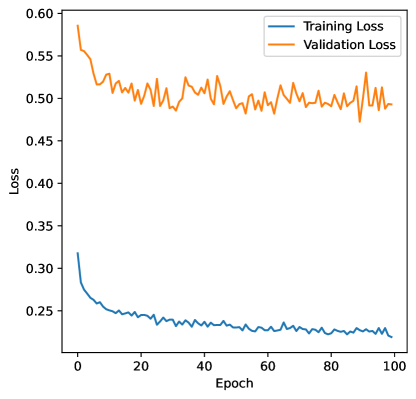
Figure 9: Training and validation loss over iterations of bilevel optimization training of Mutagenicity dataset. Even though our training process is not unstable, there is still room for improvement.

Appendix E Training Stability

To check the training stability of RAGE, we calculate the standard deviation of each experiment run as reported in Table 2. The results demonstrate that RAGE has a smaller standard deviation compared to the baselines, which shows the stability of RAGE performance.

In addition to standard deviation, we provide the change in training and validation loss over epochs. Antoniou et.al. [43] discusses the drawback of bilevel optimization algorithms in terms of stability and proposes a few modifications. Here, we provide the same analysis done in [43] for bilevel optimization training. The results show that RAGE is not significantly affected by the training instability of bilevel optimization. It could be because of the selection of inner and outer-loop epochs. However, Figure 9 shows that there is still room for improvement. The solutions provided in [43] to make the training process more stable are also applicable to our method, RAGE.

Table 8: Training and testing time for RAGE and baselines for Mutagenicity. RAGE trains slower than standard and some of the sophisticated GNN methods, while having comparable or faster testing time. For graph explainers, RAGE is comparable in training and much faster in testing.

		Training	Testing
Standard GNNs	GCN	422s	0.346s
	GAT	453s	0.345s
	GIN	442s	0.302s
	ExpertPool	433s	0.357s
	SortPool	440s	0.369s
Sophisticated GNNs	DropGNN	1143s	1.188s
	GMT	1320s	0.518s
	GIB	2716s	4.981s
	VIB-GSL	2458s	8.930s
	LDS-GNN	18793s	5.284s
	ProtGNN	15484s	0.867s
Post-hoc Explainers	PGExplainer	4585s	14.312s
	RCExplainer	12414s	48.521s
	TAGE	621s	38.625s
Our methods	RAGE	3242s	0.407s
	RAGE-Single	512s	0.407s

Appendix F Running Time

Bilevel optimization needs more training time than the standard GNNs. However, the outer update does not require a fully converged inner GNN (We use 20 inner-loop and 100 outer-loop iterations with early stopping). Furthermore, gradient estimations or momentum-based optimization can be applied [44] for faster training. Table 8 shows training and testing times for the Mutagenicity dataset for all methods. Compared to graph classification methods, RAGE has comparable or faster testing times. For post-hoc graph explainers, RAGE has comparable training time and much faster testing time. Also notice that RAGE-single has a comparable or faster training time performance to all methods while being more accurate for most datasets (check Table 2 and Table 4). RAGE-keep has same running time as RAGE except the reinitialization step which is negligible.

Appendix G More Case Studies

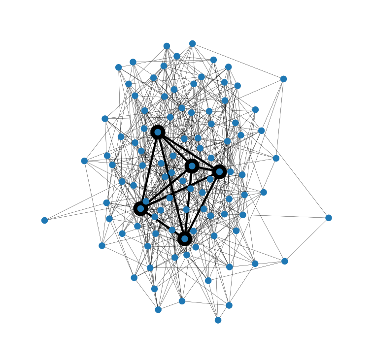
(a) Original Graph

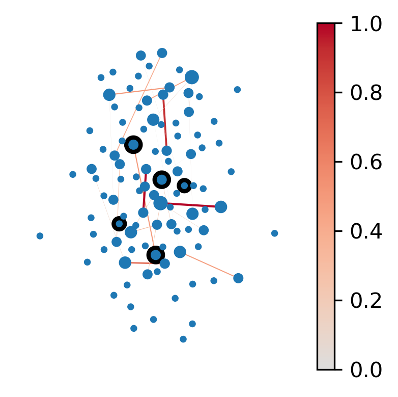
(b) GNNExplainer

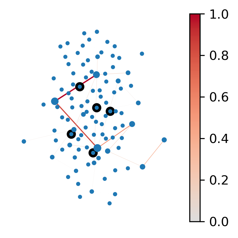
(c) PGExplainer

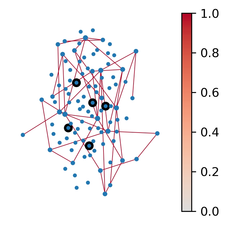
(d) SubgraphX

(e) RCExplainer

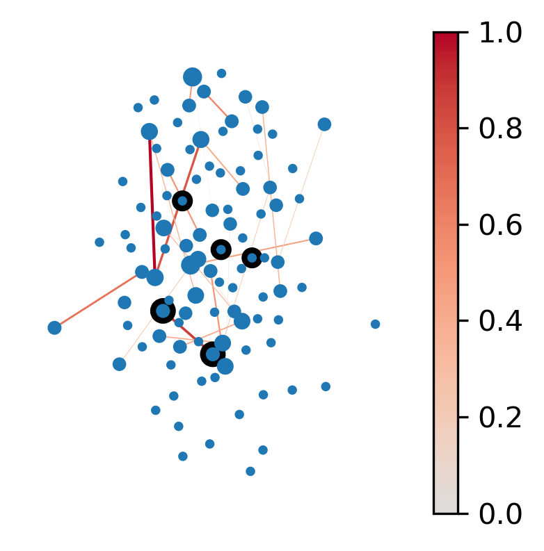
(f) TAGE

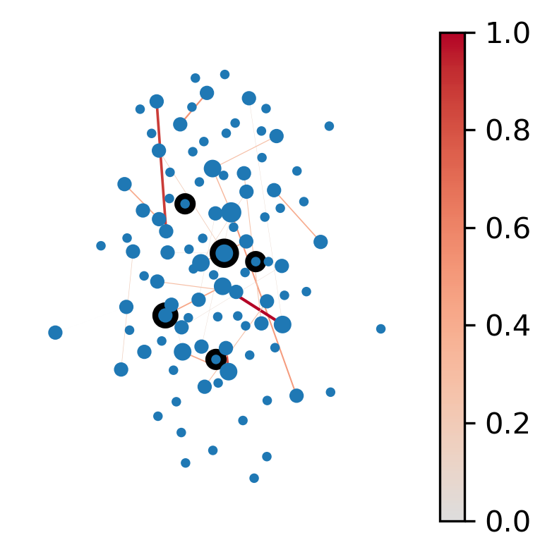
(g) CF²

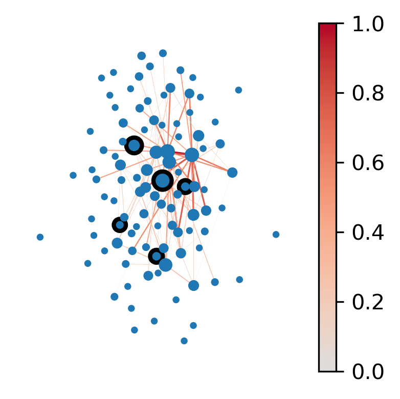
(h) GIB

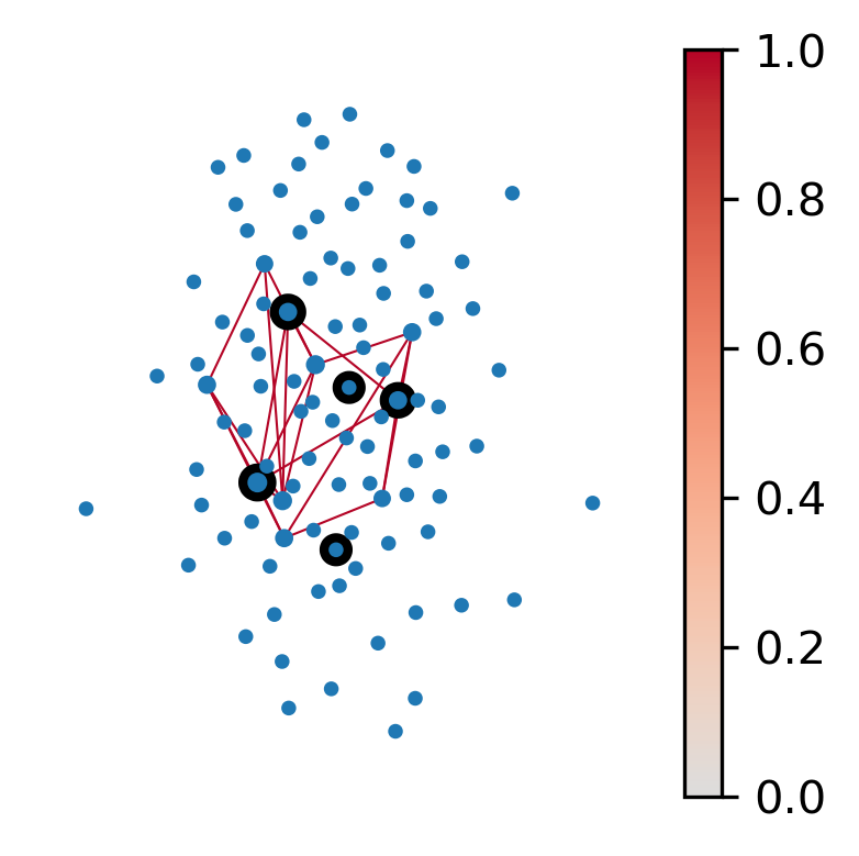
(i) ProtGNN

(j) RAGE

Figure 10: Planted Clique detection case study comparing our approach (RAGE) and several graph explainers including transductive post-hoc explainers. The five nodes in the clique are shown with a thick border. The heatmap and node sizes (edge thickness) show the node (edge) importance attributed by the explainer. As opposed to the baselines, RAGE is able to correctly detect the clique as an explanation.

Figure 10 shows our second case study (Planted Clique dataset). In this case, the explanations should contain nodes/edges in the planted clique. As GIN is the best performing basic GNN model, we use it as a base model. Notice that even though the GIN achieves good results (see Table 2), the explanations generated by the baselines do not match the clique. This behavior of post-hoc explainers is also discussed in [45, 8]. Ante-hoc explainers, GIB and ProtGNN, are the best baselines. Our approach (RAGE) is able to detect the clique as an explanation.

Appendix H More Experimental Details

H.1 Implementation:

Our implementation of RAGE is anonymously available online https://anonymous.4open.science/r/RAGE. We run and test our experiments on a machine with NVIDIA GeForce RTX 2080 GPU (8GB of RAM) and 32 Intel Xeon CPUs (2.10GHz and 128GB of RAM).

H.2 Hyperparameters:

We tune the hyperparameters of our methods and baselines with a grid search. Adam optimizer with a learning rate of $0.001$ works well in practice for our inner and outer optimization. $T$ and $\kappa$ (number of inner and outer epochs) are set to $20$ and $100$ with early stopping, respectively. We choose $0.001$ for regularization weights for inner and outer problem regularization. If the focus is only on graph classification performance, sparsity regularization weight can be set to $0$.

H.3 Model selection:

We model $g$ as a combination of a $3$-layer GCN and a $1$-layer MLP with sigmoid activation function. For the inner GNN, we use a $3$-layer influence-weighted GCN (see Section 2.2.2) and a $1$-layer MLP in our experiments. The size of the embeddings is fixed at $20$. For all graph classification and explainer baselines, we usually set the GCN layers with the same settings as ours in order to have a fair comparison (unless there are special circumstances of the baseline methods). We changed the baselines’ loss functions to mean squared error for Tree of Life datasets and removed the sigmoid activation function MLP.

H.4 Datasets Details

Table 1 shows the main statistics of the datasets used in our experiments. Mutagenicity [12, 13], Proteins [14, 15], IMDB-B [16] are graph classification datasets. We assign one-hot node degrees as features for IMDB-Binary, which originally does not have node features. Sunglasses [17] is a dataset created from the CMU face dataset, where nodes are pixels, edges connect nearby pixels, node attributes are pixel (gray-scale) colors, and labels indicate whether the person in the picture wears sunglasses. Tree of Life [18] is a collection of Protein-Protein Interaction (PPI) networks with amino-acid sequence embeddings [46] as node features and (real) evolution scores as graph labels. Planted Clique are Erdős–Rényi (ER) graphs (edge probability of 0.1) and add a planted clique of size $k$ (class 1) to half of them (others assigned to class 0). We select the value of $k$ to be larger than the size of the largest clique in the ER graphs. We also consider a noisy version of Mutagenicity, which we call MutagenicityNoisyX, where the noise $X\in\{1,2,4,8,16,32\}$ corresponds to the number of i.i.d. random edges added to each graph.

H.5 Dataset splits:

We use 80% training, 10% validation, and 10% testing splits in our experiments using random seed 0. For our method, we further split the training set into 50% training and 50% support sets. We run each method 20 times (random seeds 1-20) and report the average accuracy and standard deviation.

Appendix I Future Work, Limitations, Broader Impacts

Future Work: We will investigate how a sampling-based extension of our approach can enable the discovery of multiple plausible but independent explanations for predictions. Moreover, we will consider the semi-supervised setting for learning GNN explainers, where a small number of labeled explanations are available and/or a human-in-the-loop can evaluate explanations on demand.

Limitations: RAGE still has room for improvement on its training stability (Sec. E) and training running time (Sec. F) due to the nature of bilevel optimization. We discuss potential improvements and we aim to apply those in future work.

Broader Impacts: We do not anticipate any direct negative societal impact. However, it is possible for third parties to use our method and declare that it generates good explanations and accuracy without proper evaluation on the domain.

References

- Ying et al. [2019] Rex Ying, Dylan Bourgeois, Jiaxuan You, Marinka Zitnik, and Jure Leskovec. Gnnexplainer: Generating explanations for graph neural networks. Advances in neural information processing systems, 32:9240, 2019.
- Luo et al. [2020] Dongsheng Luo, Wei Cheng, Dongkuan Xu, Wenchao Yu, Bo Zong, Haifeng Chen, and Xiang Zhang. Parameterized explainer for graph neural network. arXiv preprint arXiv:2011.04573, 2020.
- Bajaj et al. [2021] Mohit Bajaj, Lingyang Chu, Zi Yu Xue, Jian Pei, Lanjun Wang, Peter Cho-Ho Lam, and Yong Zhang. Robust counterfactual explanations on graph neural networks. Advances in Neural Information Processing Systems, 34:5644–5655, 2021.
- Faber et al. [2020] Lukas Faber, Amin K Moghaddam, and Roger Wattenhofer. Contrastive graph neural network explanation. In ICML Workshop on Graph Representation Learning and Beyond, page 28. International Conference on Machine Learning, 2020.
- Vilone and Longo [2020] Giulia Vilone and Luca Longo. Explainable artificial intelligence: a systematic review. arXiv preprint arXiv:2006.00093, 2020.
- Yuan et al. [2022] Hao Yuan, Haiyang Yu, Shurui Gui, and Shuiwang Ji. Explainability in graph neural networks: A taxonomic survey. IEEE Transactions on Pattern Analysis and Machine Intelligence, 2022.
- Rudin [2019] Cynthia Rudin. Stop explaining black box machine learning models for high stakes decisions and use interpretable models instead. Nature Machine Intelligence, 1(5):206–215, 2019.
- Zhang et al. [2022] Zaixi Zhang, Qi Liu, Hao Wang, Chengqiang Lu, and Cheekong Lee. Protgnn: Towards self-explaining graph neural networks. In Proceedings of the AAAI Conference on Artificial Intelligence, volume 36, pages 9127–9135, 2022.
- Zhou et al. [2022] Hattie Zhou, Ankit Vani, Hugo Larochelle, and Aaron Courville. Fortuitous forgetting in connectionist networks. arXiv preprint arXiv:2202.00155, 2022.
- Alabdulmohsin et al. [2021] Ibrahim Alabdulmohsin, Hartmut Maennel, and Daniel Keysers. The impact of reinitialization on generalization in convolutional neural networks. arXiv preprint arXiv:2109.00267, 2021.
- Grefenstette et al. [2019] Edward Grefenstette, Brandon Amos, Denis Yarats, Phu Mon Htut, Artem Molchanov, Franziska Meier, Douwe Kiela, Kyunghyun Cho, and Soumith Chintala. Generalized inner loop meta-learning. arXiv preprint arXiv:1910.01727, 2019.
- Riesen and Bunke [2008] Kaspar Riesen and Horst Bunke. Iam graph database repository for graph based pattern recognition and machine learning. In Joint IAPR International Workshops on Statistical Techniques in Pattern Recognition (SPR) and Structural and Syntactic Pattern Recognition (SSPR), pages 287–297. Springer, 2008.
- Kazius et al. [2005] Jeroen Kazius, Ross McGuire, and Roberta Bursi. Derivation and validation of toxicophores for mutagenicity prediction. Journal of medicinal chemistry, 48(1):312–320, 2005.
- Borgwardt et al. [2005] Karsten M Borgwardt, Cheng Soon Ong, Stefan Schönauer, SVN Vishwanathan, Alex J Smola, and Hans-Peter Kriegel. Protein function prediction via graph kernels. Bioinformatics, 21(suppl_1):i47–i56, 2005.
- Dobson and Doig [2003] Paul D Dobson and Andrew J Doig. Distinguishing enzyme structures from non-enzymes without alignments. Journal of molecular biology, 330(4):771–783, 2003.
- Yanardag and Vishwanathan [2015] Pinar Yanardag and SVN Vishwanathan. Deep graph kernels. In Proceedings of the 21th ACM SIGKDD international conference on knowledge discovery and data mining, pages 1365–1374, 2015.
- Mitchell and Mitchell [1997] Tom M Mitchell and Tom M Mitchell. Machine learning, volume 1. McGraw-hill New York, 1997.
- Zitnik et al. [2019] Marinka Zitnik, Rok Sosič, Marcus W Feldman, and Jure Leskovec. Evolution of resilience in protein interactomes across the tree of life. Proceedings of the National Academy of Sciences, 116(10):4426–4433, 2019.
- Kipf and Welling [2016] Thomas N Kipf and Max Welling. Semi-supervised classification with graph convolutional networks. arXiv preprint arXiv:1609.02907, 2016.
- Veličković et al. [2017] Petar Veličković, Guillem Cucurull, Arantxa Casanova, Adriana Romero, Pietro Lio, and Yoshua Bengio. Graph attention networks. arXiv preprint arXiv:1710.10903, 2017.
- Xu et al. [2018] Keyulu Xu, Weihua Hu, Jure Leskovec, and Stefanie Jegelka. How powerful are graph neural networks? arXiv preprint arXiv:1810.00826, 2018.
- Zhang et al. [2018] Muhan Zhang, Zhicheng Cui, Marion Neumann, and Yixin Chen. An end-to-end deep learning architecture for graph classification. In Proceedings of the AAAI conference on artificial intelligence, volume 32, 2018.
- Li et al. [2019] Jia Li, Yu Rong, Hong Cheng, Helen Meng, Wenbing Huang, and Junzhou Huang. Semi-supervised graph classification: A hierarchical graph perspective. In The Web Conference, pages 972–982, 2019.
- Papp et al. [2021] Pál András Papp, Karolis Martinkus, Lukas Faber, and Roger Wattenhofer. Dropgnn: random dropouts increase the expressiveness of graph neural networks. Advances in Neural Information Processing Systems, 34, 2021.
- Baek et al. [2021] Jinheon Baek, Minki Kang, and Sung Ju Hwang. Accurate learning of graph representations with graph multiset pooling. In ICLR, 2021. URL https://openreview.net/forum?id=JHcqXGaqiGn.
- Yu et al. [2021] Junchi Yu, Tingyang Xu, Yu Rong, Yatao Bian, Junzhou Huang, and Ran He. Graph information bottleneck for subgraph recognition. In International Conference on Learning Representations, 2021.
- Franceschi et al. [2019] Luca Franceschi, Mathias Niepert, Massimiliano Pontil, and Xiao He. Learning discrete structures for graph neural networks. In International conference on machine learning, pages 1972–1982. PMLR, 2019.
- Sun et al. [2022] Qingyun Sun, Jianxin Li, Hao Peng, Jia Wu, Xingcheng Fu, Cheng Ji, and S Yu Philip. Graph structure learning with variational information bottleneck. In Proceedings of the AAAI Conference on Artificial Intelligence, volume 36, pages 4165–4174, 2022.
- Xie et al. [2022] Yaochen Xie, Sumeet Katariya, Xianfeng Tang, Edward Huang, Nikhil Rao, Karthik Subbian, and Shuiwang Ji. Task-agnostic graph explanations. arXiv preprint arXiv:2202.08335, 2022.
- Yuan et al. [2021] Hao Yuan, Haiyang Yu, Jie Wang, Kang Li, and Shuiwang Ji. On explainability of graph neural networks via subgraph explorations. In International Conference on Machine Learning, pages 12241–12252. PMLR, 2021.
- Tan et al. [2022] Juntao Tan, Shijie Geng, Zuohui Fu, Yingqiang Ge, Shuyuan Xu, Yunqi Li, and Yongfeng Zhang. Learning and evaluating graph neural network explanations based on counterfactual and factual reasoning. In Proceedings of the ACM Web Conference 2022, pages 1018–1027, 2022.
- Agarwal et al. [2023] Chirag Agarwal, Owen Queen, Himabindu Lakkaraju, and Marinka Zitnik. Evaluating explainability for graph neural networks. Scientific Data, 10(1):144, 2023.
- Gilmer et al. [2017] Justin Gilmer, Samuel S Schoenholz, Patrick F Riley, Oriol Vinyals, and George E Dahl. Neural message passing for quantum chemistry. In International conference on machine learning, pages 1263–1272. PMLR, 2017.
- Ying et al. [2018] Rex Ying, Jiaxuan You, Christopher Morris, Xiang Ren, William L Hamilton, and Jure Leskovec. Hierarchical graph representation learning with differentiable pooling. arXiv preprint arXiv:1806.08804, 2018.
- Gao and Ji [2019] Hongyang Gao and Shuiwang Ji. Graph u-nets. In international conference on machine learning, pages 2083–2092. PMLR, 2019.
- Mesquita et al. [2020] Diego Mesquita, Amauri Souza, and Samuel Kaski. Rethinking pooling in graph neural networks. Advances in Neural Information Processing Systems, 33:2220–2231, 2020.
- Molnar [2020] Christoph Molnar. Interpretable machine learning. Lulu. com, 2020.
- Colson et al. [2007] Benoît Colson, Patrice Marcotte, and Gilles Savard. An overview of bilevel optimization. Annals of operations research, 153(1):235–256, 2007.
- Franceschi et al. [2018] Luca Franceschi, Paolo Frasconi, Saverio Salzo, Riccardo Grazzi, and Massimiliano Pontil. Bilevel programming for hyperparameter optimization and meta-learning. In International Conference on Machine Learning, pages 1568–1577. PMLR, 2018.
- Huang and Zitnik [2020] Kexin Huang and Marinka Zitnik. Graph meta learning via local subgraphs. Advances in Neural Information Processing Systems, 33, 2020.
- Wan and Schweitzer [2021] Guihong Wan and Haim Schweitzer. Edge sparsification for graphs via meta-learning. In 2021 IEEE 37th International Conference on Data Engineering (ICDE), pages 2733–2738. IEEE, 2021.
- Zhu et al. [2021] Yanqiao Zhu, Weizhi Xu, Jinghao Zhang, Qiang Liu, Shu Wu, and Liang Wang. Deep graph structure learning for robust representations: A survey. arXiv preprint arXiv:2103.03036, 2021.
- Antoniou et al. [2018] Antreas Antoniou, Harrison Edwards, and Amos Storkey. How to train your maml. arXiv preprint arXiv:1810.09502, 2018.
- Yang et al. [2021] Junjie Yang, Kaiyi Ji, and Yingbin Liang. Provably faster algorithms for bilevel optimization. Advances in Neural Information Processing Systems, 34:13670–13682, 2021.
- Faber et al. [2021] Lukas Faber, Amin K. Moghaddam, and Roger Wattenhofer. When comparing to ground truth is wrong: On evaluating gnn explanation methods. In Proceedings of the 27th ACM SIGKDD Conference on Knowledge Discovery & Data Mining, pages 332–341, 2021.
- Yang et al. [2018] Kevin K Yang, Zachary Wu, Claire N Bedbrook, and Frances H Arnold. Learned protein embeddings for machine learning. Bioinformatics, 34(15):2642–2648, 2018.
-
•