Accelerated K-Serial Stable Coalition for
Dynamic Capture and Resource Defense

Abstract

Coalition is an important mean of multi-robot systems to collaborate on common tasks. An adaptive coalition strategy is essential for the online performance in dynamic and unknown environments. In this work, the problem of territory defense by large-scale heterogeneous robotic teams is considered. The tasks include exploration, capture of dynamic targets, and perimeter defense over valuable resources. Since each robot can choose among many tasks, it remains a challenging problem to coordinate jointly these robots such that the overall utility is maximized. This work proposes a generic coalition strategy called K-serial stable coalition algorithm. Different from centralized approaches, it is distributed and complete, meaning that only local communication is required and a K-serial Stable solution is ensured. Furthermore, to accelerate adaptation to dynamic targets and resource distribution that are only perceived online, a heterogeneous graph attention network based heuristic is learned to select more appropriate parameters and promising initial solutions during local optimization. Compared with manual heuristics or end-to-end predictors, it is shown to both improve online adaptability and retain the quality guarantee. The proposed methods are validated via large-scale simulations with $170$ robots and hardware experiments of $13$ robots, against several strong baselines such as GreedyNE and FastMaxSum.

I Introduction

Multi-robot systems can be extremely efficient when solving a team-wide task in a concurrent manner. The key to efficiency is an effective strategy for collaboration to improve overall utility, where different robots form coalitions to tackle a common task, e.g., multiple UAVs surveil an area for intruders by dividing it into respective regions [1, 2]; multiple UGVs capture an intruder by approaching from different directions [3, 4]. However, when there are a large amount of diverse tasks to be accomplished, the optimal collaboration strategy is significantly more difficult to derive, as each robot needs to choose among numerous potential coalitions, yielding a combinatorial explosion in complexity [5, 6]. Such difficulty is further amplified when the tasks is generated online non-deterministically and dynamically. In these scenarios, an adaptive collaboration strategy is essential to dynamically adjust coalitions online and re-assign robots to new tasks [7]. Furthermore, when the numbers of robots and tasks are large, a centralized coordinator that assigns coalitions centrally quickly becomes inadequate, especially for the dynamic scenario. Instead, a decentralized coalition strategy is more suitable [8, 9], where each robot coordinates with other robots via local communication.

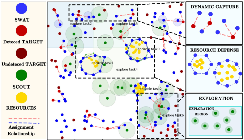
Figure 1: Snapshots of the simulated scenario: $100$ UGVs and $20$ UAVs coordinate distributedly and simultaneously three different tasks including exploration of over $50$ unknown targets and $100$ unknown resources, dynamic capture of detected targets, and defense over detected resources.

I-A Related Work

This work focuses on the particular application of deploying fleets of UAVs and UGVs for three different tasks: the exploration over a territory, the capture of potential intruders, and the defense of valuable resources. Much recent work tackles each of these tasks, e.g., the collaborative exploration or coverage problem [1, 2]; the well-known pursuit-evasion problem [3, 4, 10]; the perimeter defense problem [11]. Various extensions can be found where the team size, capability, environment model changes. For instances, an optimal pursuit strategy is designed in [12] first for the 2v2 perimeter defense problem, and then extended to NvM cases in a greedy way. The work in [13] employs a graph-theoretic approach to ensure the distance-based observation graph remains connected, i.e., the evaders are always visible. A flexible strategy is proposed in the recent work [14], which can enclose and herd evaders to designated areas. The work in [15] proposes an encirclement strategy for the slow pursuers to capture the faster evader. However, these tasks are often considered separately and individually in the aforementioned work. Thus, the proposed methods therein can not be applied directly when the same team of heterogeneous robots are responsible for a dynamic combination of these three tasks.

On the other hand, the task assignment for multi-agent systems refers to the process of assigning a set of tasks to the agents, see [16, 17] for comprehensive surveys. Well-known problems include the classic one-to-one assignment problem [18], the multi-vehicle routing problem [17], and the coalition structure generation (CSG) problem [19]. Representative methods include the Hungarian method [18], the mixed integer linear programming (ILP) [16] and the search-based methods [20]. However, these methods typically rely on the static table of agent-task pairwise cost. Such cost matrix does not exist for any of three tasks considered here. More specifically, the benefit of one robot joining a coalition depends mainly on other robots that are already in the coalition, which often decreases drastically as more robots join the same coalition. Consequently, these existing methods for task assignment are not suitable for this application.

Lastly, the CSG problem mentioned above is the most relevant as it is particularly suitable for collaborative tasks, see the comprehensive study in [6]. A marketed-based coalition formation algorithm is presented in [21], with no clear guarantee on the solution quality. Provably optimal algorithms are proposed in [5], which have not been applied to large-scale systems due to combinatorial complexity. Thus, distributed and anytime approaches are proposed in [8, 9], which are designed to solve static coalition formation problems. Notably, learning-based methods are proposed in [22, 23] to learn via reinforcement learning or supervised learning to mimic an expert solver. However, the learned heuristic in this work is used to accelerate the model-based planning algorithm, instead of replacing it as a black-box predictor. In other words, the theoretical guarantee on solution quality is retained.

I-B Our Method

To overcome these limitations, this work proposes a distributed coalition strategy for heterogeneous robots under the tasks of dynamic capture and resource defense. Its backbone is the K-serial stable coalition algorithm (KS-COAL), which is a distributed and complete algorithm designed for generic definition of collaborative tasks. It is particularly suitable for large-scale robotic teams under unknown and dynamic environments, where the tasks are generated and changed online. Model-based motion strategies and utility functions are designed for generic tasks, which are adaptive to team sizes and environment features. It is proven formally to be complete and strictly better than the popular Nash-one-stable solutions. To further improve the solution quality within a limited computation time, the KS-COAL algorithm is accelerated by choosing more promising initial solutions and better parameters, which are learned offline based on optimal solutions of small-scale problems and use heterogeneous graph attention networks (HGAN) as the network structure. Consequently, the learned heuristics are integrated seamlessly with the KS-COAL algorithm. The proposed method is validated extensively on large-scale simulations against strong baselines.

Main contributions of this paper are summarized as follows: (i) an unified framework for distributed task coordination of multi-agent systems under diverse tasks; (ii) a coordination algorithm with provable guarantee of quality; (iii) a supervised learning mechanism to accelerate the online coordination process, without losing the quality guarantee.

II Problem Description

II-A Workspace and Robot Description

Consider a group of robots $\mathcal{R}$ that co-exist in a common workspace $\mathcal{W}\subset\mathbb{R}^{2}$. Each robot $i\in\mathcal{R}$ is described by three components: (i) Motion model. Each robot follows the unicycle model with state $s_{i}$ as the 2D coordinates and orientation, and input $u_{i}$ as the angular and linear velocities; (ii) Perception model. Each robot can observe fully the environment within its sensing radius $r_{i}>0$; (iii) Action model. There are three teams of robots with distinctive capabilities: (i) SCOUT team $\mathcal{R}_{\texttt{o}}\subset\mathcal{R}$ that moves swiftly and is capable of long-range perception; (ii) SWAT team $\mathcal{R}_{\texttt{c}}\subset\mathcal{R}$ that is capable of short-range perception but specialized for capturing other robots that are less than $d_{\texttt{c}}>0$ in distance; and (iii) TARGET team $\mathcal{R}_{\texttt{s}}\subset\mathcal{R}$ that is capable of mid-range perception and can take “resources” within the workspace that are less than $d_{\texttt{s}}>0$ in distance. In other words, the scout robots, typically UAVs, can navigate easily around the workspace to locate any target robot and resources, such that the swat robots, typically UGVs, can approach and capture the target robots or form encirclement to defend resources.

Lastly, it is assumed that robots within the scout team can communicate freely without any range limitation, the same applies to robots within the target team. However, they can not eavesdrop over other teams communication. All swat robots communicate locally within a limited range, and the overall communication network is connected infinitely often.

II-B Resource Generation

To mimic the task of perimeter defense with valuable resources, it is assumed that one resource $\xi_{t}$ is generated every period $T_{r}>0$ around several clusters within the workspace, following a Gaussian Mixture Model (GMM) e.g., $\xi_{t}\sim\texttt{GMM}(\{(\alpha_{k},\mu_{k},\Sigma_{k})\})$, where $(\alpha_{k},\mu_{k},\Sigma_{k})$ are the weight, mean and covariance of Gaussian component $G_{k}$. The distribution of these clusters is static but unknown initially, thus can only be estimated online. After generation, one resource remains available until it is taken by a target robot. New resources are constantly generated by the distribution above. Denoted by $\Xi_{t}$ the set of resources that are available at time $t\geq 0$, which is set to $\emptyset$ initially. Meanwhile, each target robot $i\in\mathcal{R}_{\texttt{s}}$ searches for resources via random exploration. Once found, the robot approaches the resource via the shortest path and takes it if available, while avoiding being captured by the swat team. If a target robot is captured, it is immobilized and can not take resources anymore.

II-C Problem Formulation

The overall objective is to design a distributed control strategy for the scout and swat teams, such that the number of captured target robots subtracting the number of resources taken by the target team is maximized.

Remark 1.

The desired strategy is distributed, meaning that there exist no central coordinator that assigns globally the next control and action for each robot. Instead, the scout and swat robots synthesize the best strategy for the team collaboratively, via local communication and coordination. $\blacksquare$

III Proposed Solution

The proposed solution is a distributed framework for task coordination and motion control. It consists of three main components: (i) the motion strategies for all robots are introduced in Sec. III-A; (ii) the distributed coordination algorithm KS-COAL is described in Sec. III-B; (iii) a HGAN-based accelerator for the distributed algorithm is designed in Sec. III-C.

III-A Task Definition and Motion Strategy

This section describes three different types of tasks and the associated motion strategies as illustrated as shown in Fig. 2. Particularly, the online detection of target robots and resources by the scout robots is achieved by partitioning the workspace and solving a minimum-time coverage problem [1, 2]. Capture of target robots by the swat robots follows the dynamic strategy of computing online the intersection of Apollonius circles [3, 4]. Encirclement of resources by the swat robots is solved as formation problem given the distribution of resources [11, 15]. The target teams follows the strategy as described in Sec. II-B. Additionally, a utility function is defined for possible coalitions w.r.t. each task to measure the required time, which serves as a fundamental component for the coalition formation algorithm later. Due to limited space, details of the task definition and associated motion strategies are omitted and can be found in the supplementary file.

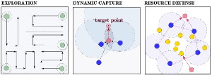
Figure 2: Illustration of the motion strategies for three different tasks.

III-B Distributed Coalition Formation

Given the above three types of tasks and the associated utility function described in Sec. III-A, the next prominent step is to form coalitions within the team of swat and scout robots such that the overall utility for the team is optimized. Different from most relevant work that focuses on a centralized solution for static scenes, this work proposes a unified, complete and distributed algorithm that can handle a large number of diverse tasks in dynamic environments.

III-B1 Problem Reformulation

To begin with, the task assignment problem is formulated based on the coalition formation literature [6, 7]. Particularly, consider the following definition of a coalition structure:

$$\mathcal{F}\triangleq(\mathcal{R},\,\Omega,\,f,\,\mathcal{K}),$$ (1)

where $\mathcal{R}=\{1,\cdots,N\}$ is the team of $N$ robots; $\Omega=\{\omega_{1},\cdots,\omega_{M}\}$ is the set of $M$ tasks; $f:2^{\mathcal{R}}\times\Omega\rightarrow\mathbb{R}^{+}$ is the utility function of a potential coalition for any given task in $\Omega$; $\mathcal{K}=\{k_{1},\cdots,k_{N}\}$ is the optimality index designed for limiting the communication and computation complexity for each robot, which is assumed to be static for now but adaptive in the overall algorithm presented in the sequel. The set of tasks that can be performed by robot $i$ is denoted by $\Omega_{i}$.

Definition 1 (Assignment).

A valid solution of the coalition structure $\mathcal{F}$ in (1) is called an assignment, denoted by $\nu=\{(\omega_{m},\,\mathcal{R}_{m}),\,\forall\omega_{m}\in\Omega\}$, where $\mathcal{R}_{m}\subset\mathcal{R}$ represents a coalition that performs the common task $\omega_{m}\in\Omega$, and $\mathcal{R}_{m_{1}}\cap\mathcal{R}_{m_{2}}=\emptyset,\,\forall m_{1}\neq m_{2}$. Moreover, an assignment is called optimal if its mean utility, i.e.,

$$\varrho(\nu)\triangleq\frac{\Sigma_{\omega_{m}\in\Omega}\,f(\mathcal{R}_{m},\,\omega_{m})}{M},$$ (2)

is maximized, and denoted by $\nu^{\star}$. $\blacksquare$

Note that the mean utility above is chosen to be consistent with the main objective, and resembles the overall success rate in dynamic scenes. With a slight abuse of notation, let $\nu(\omega_{m})=\mathcal{R}_{m}$ which returns the coalition for task $\omega_{m}$ and conversely, $\nu(i)=\omega_{m}$ which returns the task assigned to robot $i$, $\forall i\in\mathcal{R}_{m}$. More importantly, an assignment $\nu$ can be modified via the following switch operation by any robot.

Definition 2 (Switch Operation).

The operation that robot $i\in\mathcal{R}$ is assigned to task $\omega_{m}\in\Omega$ is called a switch operation, denoted by $\xi^{m}_{i}$. The switch $\xi^{m}_{i}$ is valid only if $\omega_{m}\in\Omega_{i}$. Thus, via $\xi^{m}_{i}$, an assignment $\nu$ is changed into a new assignment $\hat{\nu}$, such that $\hat{\nu}(i)=\omega_{m}$. For brevity, denote by $\hat{\nu}=\xi^{m}_{i}(\nu)$. $\blacksquare$

Definition 3 (Chain Transformation).

A transformation is defined as a chain of allowed switches, i.e.,

$$\Xi\triangleq\xi_{i_{1}}^{m_{1}}\circ\xi_{i_{2}}^{m_{2}}\circ\xi_{i_{\ell}}^{m_{\ell}}\cdots\circ\xi_{i_{L}}^{m_{L}},$$ (3)

where $L$ is the total length; $i_{\ell+1}\in\mathcal{N}_{\ell}$ is the constraint of forming a chain, $\forall\ell=0,\cdots,L-1$. The transformation $\Xi$ is valid if all switches inside are valid. Thus, via $\Xi$, an assignment $\nu$ can be transformed into a new assignment $\hat{\nu}$, by recursively applying the switches $\xi_{i_{\ell}}^{m_{\ell}}\in\Xi$, such that $\hat{\nu}(i_{\ell})=\omega_{m_{\ell}}$, $\forall\ell=0,\cdots,L-1$. For brevity, denote by $\hat{\nu}=\Xi(\nu)$. $\blacksquare$

Definition 4 (Rooted Transformation).

A rooted transformation at robot $i\in\mathcal{R}$ is denoted by $\Xi_{i}$, which is a chain transformation that starts from $i$, i.e., $i_{1}=i$ in (3). $\blacksquare$

Remark 2.

The chain transformation above is different from “arbitrary modification” in [7], where the sequence of transformations can be operated on any robot. However, the chain structure in (3) requires that only neighboring robots can perform switches consecutively. The main motivation is to limit the search space of possible transformations to robots within the $K$-hop local communication network, thus accelerating the convergence to a high-quality solution. $\blacksquare$

Definition 5 ($\mathcal{K}$-Serial Stable).

An assignment $\nu^{\star}$ is $\mathcal{K}$-Serial stable (KSS), if for each robot $i\in\mathcal{R}$, there does not exist any rooted transformation $\Xi_{i}$ such that: (i) $\Xi_{i}$ is valid; (ii) $\varrho(\Xi_{i}(\nu^{\star}))>\varrho(\nu^{\star})$; (iii) $|\Xi_{i}|\leq k_{i}$, where $k_{i}$ is the optimality index defined in (1). $\blacksquare$

Remark 3.

The above notion of KSS solution contains the Nash equilibrium in [7] and the globally optimal solution as special cases. Namely, if the indices are chosen that $k_{i}=1$, $\forall i\in\mathcal{R}$, then the KSS solution is equivalent to the Nash equilibrium as at most one robot is allowed to switch its own task. If $k_{i}=N$, $\forall i\in\mathcal{R}$ and the communication graph is connected, then the KSS solution is equivalent to the globally optimal solution as all robots can switch tasks simultaneously. Thus, the parameter $\mathcal{K}=\{k_{i}\}$ provides the flexibility to adaptively improve the solution given the time budget. $\blacksquare$

Problem 1.

Given the coalition structure $\mathcal{F}$ in (1), design a distributed algorithm to find one KSS solution by Def. 5. $\blacksquare$

III-B2 Algorithm Description

A distributed, asynchronous and complete algorithm called the $\mathcal{K}$-serial stable coalition (KS-COAL) is proposed to solve Problem 1. As shown in Fig. 3, the main idea is to combine distributed communication and local optimization. Each robot $i$ attempts to find the locally-best transformation rooted at itself, which can improve the currently-known best solution the most. In addition, each robot also participates in the optimization of transformations rooted at other robots, i.e., as part of the chain defined in (3). Lastly, a consensus protocol is running in parallel to encourage the convergence to a common KSS solution across the team.

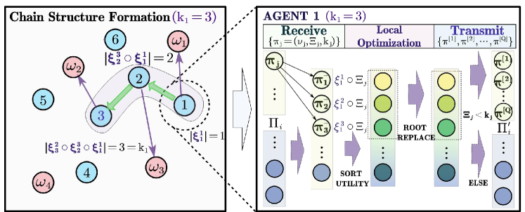
Figure 3: Illustration of key steps in the KS-COAL algorithm: distributed exchange via the chain structure (left) and local optimization (right).

More specifically, as summarized in Alg. 1, each robot follows the same algorithmic procedure asynchronously. At $t=0$, each robot computes the set of initial partial solutions by assigning one task to itself, as its local information. Then, robot $i$ sends the message below to all its neighbors $j\in\mathcal{N}_{i}$:

$$\pi_{i\rightarrow j}\in\{(\nu_{0},\,\varepsilon,\,k_{i}),\;\nu_{0}(i)=\omega_{m}\in\Omega_{i}\},$$ (4)

where $\nu_{0}$ is the partial solution; $\varepsilon$ denotes the null transformation and $k_{i}$ is the optimality index of robot $i$. This message is added to a local message buffer denoted by $\Pi_{i}$, see Line 1.

At $t>0$, each robot $i\in\mathcal{N}$ follows the same round of receiving messages, local optimization, sending messages, and consensus, as in Lines 1-1. To begin with, for any stored message $\pi=(\nu,\,\Xi,\,k)\in\Pi_{i}$ that $|\Xi|\leq k$ holds, robot $i$ relays this message to its neighbors, i.e., $\pi_{i\rightarrow j}=\pi$, $\forall j\in\mathcal{N}_{i}$. Meanwhile, after receiving each message $\pi_{j\rightarrow i}$ from robot $j$ that $i\in\mathcal{N}_{j}$, it stores $\pi_{j\rightarrow i}$ in its buffer $\Pi_{i}$. During local optimization, robot $i$ generates a new message $\pi^{+}$ for any selected message $\pi=(\nu,\,\Xi,\,k)\in\Pi_{i}$ by appending an additional switch operation for each task $\omega_{m}\in\Omega_{i}$ to the existing transformation, i.e.,

$$\pi^{+}=(\nu,\,\Xi\circ\xi^{m}_{i},\,k),\,\forall\omega_{m}\in\Omega_{i};$$ (5)

where $\nu$ is the same initial solution as in $\pi$; $\xi^{m}_{i}$ assigns robot $i$ to task $\omega_{m}$. Note that this modification is only allowed if $|\Xi|\leq k$, i.e., its length limit is not reached. This new message $\pi^{+}$ is stored in $\Pi_{i}$, see Line 1-1. More importantly, robot $i$ maintains the best assignment that is known to itself, denoted by $\nu^{\star}_{i}$. It is updated each time a message is received or a new message is generated in (5), i.e.,

$$\nu^{\star}_{i}=\Xi(\nu),\quad\text{if}\;\rho(\Xi(\nu))>\rho(\nu^{\star}_{i}),$$ (6)

as in Line 1, where the updated utility $\rho(\Xi(\nu))$ can be computed locally by robot $i$ as $\rho(\Xi(\nu))=\rho(\nu^{\star}_{i})+\Delta_{f}(\omega_{m})+\Delta_{f}(\omega^{\prime}_{m})$, where $\omega_{m},\,\omega^{\prime}_{m}$ are tasks assigned to robot $i$ before and after the update, respectively; and $\Delta_{f}(\cdot)$ is the difference in task utility of $\omega_{m},\,\omega^{\prime}_{m}$ before and after the update.

Input: Coalition structure $\mathcal{F}$.

Output: KSS solution $\nu^{\star}$.

/* Message passing */

1 Initialize $\Pi_{i}$ by (4),   $\Pi^{\star}_{i}=\emptyset$ ;

2 while not terminated do

       /* Sending message */

3       for $\pi=(\nu,\,\Xi,\,k)\in\Pi_{i}$ and $|\Xi|\leq k$ do

4             Send $\pi_{i\rightarrow j}$ to $\mathcal{N}_{i}$;

5             Remove $\pi_{i\rightarrow j}$ from $\Pi_{i}$;

      /* Receiving message */

6       forall $i\in\mathcal{R}$ do

7             Receive $\{\pi_{j\rightarrow i}\}$ and update $\Pi_{i}$;

      /* Local optimization */

8       for $\pi=(\nu,\,\Xi,\,k)\in\Pi_{i}$ do

9            Compute $\xi_{i}^{m}$ and $\pi^{+}$ by (5);

10             Save $\pi^{+}$ to $\Pi_{i}$;

11             Update $\nu_{i}^{\star}$ by (6);

       /* Consensus */

12       if $\varrho(\nu_{j}^{\star})>\varrho(\nu_{i}^{\star})$ then

13             $\nu_{i}^{\star}\leftarrow\nu_{j}^{\star}$;

14             Compute $\{\Xi_{i}(\nu^{\star}_{i})\}$ and update $\Pi_{i}$ by (7);

15             Update $\nu_{i}^{\star}$ by (6);

16            

17      

Algorithm 1 KS-COAL algorithm.

As mentioned earlier, a consensus protocol is executed in parallel, such that the team converges to the same KSS solution. However, this should be done in special care to avoid pre-mature termination and over-constrained search space. In particular, each robot $i$ shares its best solution $\nu^{\star}_{i}$ in (5) with its neighbors, i.e., by sending directly the associated message $\pi^{\star}_{i}$, then robot $i$ can locally compute the best assignments received from other robots, namely, $\rho(\nu^{\star}_{j})$ as in Line 1. Afterwards, robot $i$ updates its best assignment if any received assignment yields a better overall utility, i.e., $\rho(\nu^{\star}_{j})>\rho(\nu^{\star}_{i})$. Then, all rooted transformations $\{\Xi_{i}\}$ stored in $\Pi_{i}$ should be applied to $\nu^{\star}_{i}$ to generate new solutions $\{\Xi_{i}(\nu^{\star}_{i})\}$, i.e.,

$$(\nu,\,\Xi_{i},\,k_{i})\rightarrow(\nu^{\star}_{i},\,\Xi_{i},\,k_{i}),$$ (7)

as in Line 1. Meanwhile, these invalid messages are removed from $\Pi_{i}$. Thus, the new assignment is given by $\Xi_{i}(\nu^{\star}_{i})$, of which the utility is computed by tracing back the chain operations in $\Xi_{i}=\xi^{m_{1}}_{i_{1}}\circ\xi^{m_{2}}_{i_{2}}\cdots\circ\xi^{m_{L}}_{i_{L}}$ and querying each robot $i_{\ell}$ along the chain directly the change of utility. If any of these new assignments in $\{\Xi_{i}(\nu^{\star}_{i})\}$ yields a better utility than $\nu^{\star}_{i}$, it replaces $\nu^{\star}_{i}$ and is shared with the neighbors, see in Line 1. If the local best assignment $\nu^{\star}_{i}$ remains unchanged after a certain number of rounds, the algorithm terminates. Note that the above algorithm is anytime, meaning that it can be interrupted anytime given the limited computation resources and still yield the currently-best solution.

III-B3 Performance Analysis

Under the proposed algorithm, convergence to a KSS solution is ensured. Furthermore, it is shown that this solution extends naturally to the globally optimal solution if $\mathcal{K}$ is set accordingly. Proofs are omitted here and provided in the supplementary file.

Theorem 1.

Under Alg. 1, the local assignment is ensured to converge to $\nu^{\star}_{i}=\nu^{\star}$, $\forall i\in\mathcal{R}$, where $\nu^{\star}$ is a KSS solution.

Corollary 1.

Given that $k_{i}=N$, $\forall i\in\mathcal{R}$, the KSS solution return by Alg. 1 is the globally optimal solution.

III-C Neural Accelerator for Dynamic Adaptation

Since all robots are constantly moving and resources are generated dynamically, the current assignment might not be optimal or even infeasible at latter time. In many cases only a few robots need to adjust their assignments. Thus, a neural accelerator (NAC) based on heterogeneous graph attention networks (HGAN) from [24] is proposed to accelerate the proposed KS-COAL, by predicting directly the choice of parameter $\mathcal{K}$ and an initial solution for KS-COAL.

III-C1 Network Structure of NAC

As shown in Fig. 4, the proposed HGAN model contains two branches called HGAN-K and HGAN-Init, which are used to predict the $\mathcal{K}$ and $\nu_{0}$, respectively. They both share the common two HGAN middle-layers to extract the hidden embedding. As inputs to both branches, two labeled graphs are constructed based on the same underlying coalition structure. In particular, three types of robots and three types of tasks are encoded as vertices with different attributes. Undirected edges from robots to tasks indicate whether one robot can participate in one task. Both node and edge attributes are encoded differently within HGAN-K and HGAN-Init: (i) The attribute of each edge in HGAN-K is a vector of marginal utility given by:

$$\upsilon_{m}(i,\omega_{m})=\left\{f(\mathcal{R}_{m},\,\omega_{m})-f(\mathcal{R}_{m}\backslash\{i\},\,\omega_{m}),\,\forall\mathcal{R}_{m}\in\widehat{\mathcal{R}}_{m}\right\},$$

where $i\in\mathcal{R}_{m}$ is any coalition that can perform task $\omega_{m}\in\Omega$; $\widehat{\mathcal{R}}_{m}\subset 2^{\mathcal{R}}$ is the set of all such coalitions; $\upsilon\in\mathbb{R}^{|\widehat{\mathcal{R}}_{m}|}_{\geq 0}$ is a vector of non-negative reals. However, the edges for HGAN-Init are attribute-free and are only responsible for passing messages. (ii) Each vertex in HGAN-K is labeled by their robot or task type. However, each vertex in HGAN-Init is encoded by stacking $\upsilon_{m}(i,\omega_{m})$ above for all possible tasks. Zero-padding is applied to ensure that these attributes have consistent sizes across vertices and edges. These graphs are then processed by the HGANs tailored for heterogeneous graphs with varying sizes. The HGAN-K outputs the predicted parameter $\mathcal{K}$ over each robot vertex, while HGAN-Init outputs a ranking over all edges of each robot vertex. More details of the adopted HGAN structure can be found in the supplementary file.

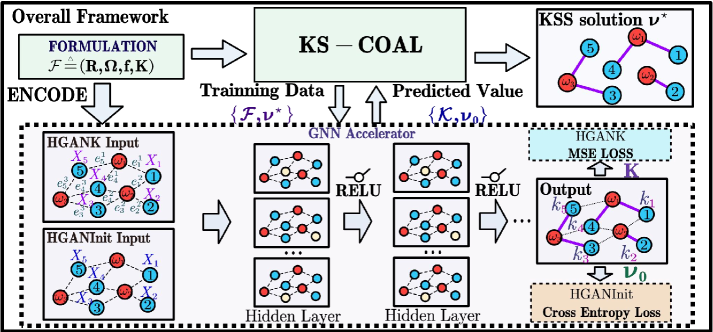
Figure 4: Network structure of the proposed NAC: the HGAN-K branch (upper) and the HGAN-Init branch (lower) that predicts the parameter $\mathcal{K}$ and initial solution $\nu_{0}$, which are used to accelerate the KS-COAL algorithm.

III-C2 Training and Execution

To begin with, the training data is collected by solving the considered scenario by the proposed KS-COAL, under different random seeds. More specifically, it is given by $\mathcal{D}=\{(\mathcal{F},\,\mathcal{K},\,\nu^{\star})\}$, where the tuple consists of a problem instance $\mathcal{F}$ in (1) under a random choice of $\mathcal{K}$; $\mathcal{K}$ is the optimal choice for each robot, and the associated KSS assignments $\nu^{\star}$ obtained by KS-COAL. First, each problem instance is transformed into labeled graphs as described above, while the optimal robot-task pairs are derived from $\nu^{\star}$ and the optimal choice of $\mathcal{K}$ is quantized into $\{1,2,3\}$ given $J^{\star}$, where $J^{\star}\in\mathbb{Z}^{N}$ is the total number of switches that each robot $i\in\mathcal{N}$ has performed and resulted in an increase of the overall utility. Then, the HGAN-K and HGAN-Init branches are both trained in a supervised way, where the “weighted MSE loss” is chosen as the loss function for HGAN-K to avoid imbalanced data, and the “Cross Entropy loss” for HGAN-Init. Note that during training, the modern HGANs recursively update the node and edge features by aggregating information from multiple-hop neighbors. Consequently, the trained HGAN-K can predict the optimal choice of $\mathcal{K}$, while the HGAN-Init outputs directly a recommended solution $\nu_{0}$.

During execution, each robot constructs its local multi-hop graphs given a new problem $\mathcal{F}$, which is encoded in the same way as the training process. Then, this labeled local graph is fed into the learned HGAN to obtain the hidden embedding, which is then aggregated via local communication with neighboring robots. Consequently, after convergence, the aggregated embedding is used to predicate the optimal choice of $k_{i}$ and $\omega_{m}$ for each robot $i\in\mathcal{N}$. Thus, the KS-COAL algorithm can be kick-started with this choice of $\mathcal{K}$ and this initial assignment $\nu_{0}$. It is worth mentioning that the guarantee on solution quality in Theorem 1 is still retained.

III-D Computation Complexity

Since Alg. 1 is fully distributed, its complexity is analyzed for a single robot. For one round of communication, robot $i$ can send at most $|\Pi_{i}|$ messages to $|\mathcal{N}_{i}|$ robots. Thus, the worst time-complexity for sending messages is $\mathcal{O}(N_{\Pi}N_{r})$, where $N_{\Pi}$ is the upperbound of $|\Pi_{i}|$ and $N_{r}<N$ is the upperbound of $|\mathcal{N}_{i}|$. Similarly, the stage of “local optimization” has the time-complexity $\mathcal{O}(N_{\Pi}N_{\omega})$, where $N_{\omega}$ is the maximum number of the tasks that one robot is capable. Thus, the overall time-complexity at each iteration is $\mathcal{O}(N_{\Pi}(2N_{r}+N_{\omega}))$. Note that $N_{\Pi}$ is upper bounded by $\left(N_{\omega}N_{r}\right)^{k_{\max}}$, where $k_{\max}=\max_{i}\,\{k_{i}\}$. Furthermore, since the exact time of convergence $\bar{t}$ is hard to determine, a factor $\epsilon$ is introduced to relax the convergence criterion. More specifically, it can be regarded as “convergence” if there is no $\Xi$ that can improve the utility $\rho$ by more than $\epsilon$. For a single robot, the number of effective switches is upper bounded by $\Delta\rho/\epsilon$, where $\Delta\rho$ is the upper bound of $\rho^{\star}-\rho$. Since the iterations required for “consensus” is bounded by $N$ between two effective switches, it holds that $\bar{t}\leq\frac{\Delta\rho}{\epsilon}N$. Thus, the overall time-complexity of Alg. 1 is given by $\mathcal{O}((N_{\omega}N_{r})^{k_{\max}}(2N_{r}+N_{\omega})(\Delta\rho/\epsilon)N)$.

Figure 5: Snapshot of the task execution: motion of all robots (left), dynamic task assignment (middle), estimated distribution of resources and targets (bottom-right), number of captured targets and resources (top-right).

IV Numerical Experiments

Extensive numerical experiments are conducted for large-scale systems, which are compared against several strong baselines. The proposed method is implemented in Python3 with Pytorch geometric Graph (PyG) from [25] and tested on an AMD 7900X 12-Core CPU @ 4.7GHz with RTX-3070 GPU. More detailed descriptions and experiment videos can be found in the supplementary file.

IV-A Setup

IV-A1 Agent and Workspace Model

As shown in Fig. 5, consider $100$ swat robots, $20$ scout robots, and $50$ target robots in a free workspace of size $100m\times 100m$. Their reference velocities are set to $1m/s$, $6m/s$ and $0.9m/s$. The sensing radius is set to $5m$ for swat robots and $10m$ for scout robots. The capture range of swat and target robots are set to $3m$ and $2m$. Moreover, the resources are generated by three Gaussian clusters of variance $0.75m$ every $5s$. Note that the initial distribution of target robots and resources are unknown to the swat and scout robots. Captured targets and taken resources are removed from display. In addition, the workspace is divided into $9$ regions for the exploration task. The proposed method is triggered by specific events and at regular intervals, specifically when targets are captured and every $5$ time steps. Detailed descriptions can be found in supplementary file.

IV-A2 Proposed Method and Baselines

The detailed setup of the proposed NAC is omitted here and provided in supplementary file. In total 10 baselines are compared: (i) the KS-COAL algorithm with the parameter $\mathcal{K}$ uniformly set to $2$, $3$, $4$ or randomly, denoted by KS2, KS3, KS4 and Random, respectively; (ii) two variants of the NAC for ablation study: NACK that only uses the learned accelerator to predict $\mathcal{K}$ with the initial solution being the previous solution, and NACInit that only predicts the initial solution with a random $\mathcal{K}$; (iii) two state-of-the-art methods for distributed coordination: GreedyNE from [9], where a Nash-stable assignment is selected; FastMaxSum from [26], which solves the matching problem over a task-robot bipartite graph via distributed message passing. (iv) two end-to-end learning paradigms are implemented, i.e., reinforcement learning from [22] and supervised learning from [23], denoted by RL and HGAN.

IV-B Results and Comparisons

IV-B1 Overall Performance

As illustrated in Fig. 5, the robot motion and actions are monitored during execution, along with the dynamic task assignment. In addition, the detected targets and resources are shown with the number of captured targets and preserved resources. Note that each time the proposed NAC is triggered, $20$ rounds of communication are allowed within the team. It can be seen that the scout robots are assigned to different partitions of the workspace. Three clusters of resources are gradually identified. Once the swat robots receive the position of target robots from the scout robots, coalitions are formed dynamically to capture target robots and form encirclement around the clusters of resources. Note that some swat robots become immobile when the marginal utility of joining a capture or defense task is negligible. Also, swat robots may switch from a defense task to a capture task, when some target robots are nearby. In total, $50$ resources are kept and $234$ target robots are captured over $200$ time steps.

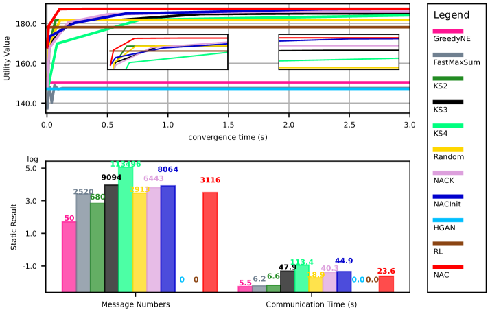
Figure 6: Evolution of the overall utility along with the computation time for our method NAC and $10$ other baselines (top); the associated total number of messages and the time of communication (bottom).

IV-B2 Convergence over a Fixed Problem

To begin with, the baselines are compared to solve the same static coalition problem, formulated based on one snapshot of dynamic scene above. Although the end-to-end predictors by RL and HGAN do not require communication, the overall performance is much lower than KS4 and NAC (147, 178 vs. 185.2, 187). All baselines are given the same number of computation and communication rounds. Evolution of the total utility along with the iterations is shown in Fig. 6. Our method NAC has a faster convergence than both KS2, KS3 and KS4 ($0.5s$ vs. $1s$, $3s$ and $20s$), but with the highest utility after convergence ($187$ vs $181$, $185$ and $185.2$). It confirms our analyses that larger $\mathcal{K}$ requires longer sequence of transformation and thus slower to converge. The proposed NAC predicts $\{k_{i}\}$ non-uniformly and accelerates the convergence even further with a good initial solution. Note that since KS4 can not converge at each iteration under limited computation time, it achieves an utility less than NAC. Both GreedyNE and FastMaxSum reach convergence within only $0.1s$ and $0.2s$, however with a final utility significantly less than KS4 and NAC ($150$, $147$ vs. $185.2$, $187$). Lastly, compared with NAC, NACK converges slower ($2s$) with a worse utility ($186$). Although trained by data from KS3, NACInit outperforms KS3 by a higher initial and final utility ($185$ and $187$). This verifies that both the parameter $\mathcal{K}$ and the initial solution $\nu_{0}$ are worth learning to accelerate the coordination.

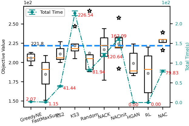
Figure 7: Overall utility and total time elapsed in dynamic scenes.

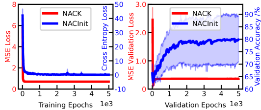
Figure 8: Training loss (left) and validation loss (middle) for HGAN-K and HGAN-Init; training reward for method RL [22] (right).

IV-B3 Communication Overhead

All methods are executed for $20$ iterations and the total amount of exchanged messages is compared. As shown in Fig. 6, it is clear that drastically more messages are generated as the parameter $\mathcal{K}$ increases i.e., $50$, $680$, $9094$ and $113496$ for GreedyNE, KS2, KS3 and KS4, respectively. Both NACK and NACInit generate less messages than KS4 ($6443$ and $8064$ vs. $113496$), due to either smaller $\mathcal{K}$ or faster convergence. Notably, our NAC requires merely $3116$ messages to reach convergence, drastically less than both variants NACK and NACInit. This signifies the effect of acceleration via the NAC. Lastly, FastMaxSum requires more messages than KS2 but less than KS4 however with different structure. Note that although KS4 yields a higher utility, it takes $6$ times more time and $12$ times more messages compared with KS3. Thus, KS4 is unsuitable for real-time applications in dynamic scenarios as discussed below.

IV-B4 Long-term Performance over Dynamic Scenes

The described experiment is repeated $10$ times with different random seeds for $200$ time steps. As summarized in Fig. 7, our NAC drastically improves the accumulated performance by $11\%$ in average compared with GreedyNE, $24\%$ than FastMaxsum, $15\%$ than HGAN and $23\%$ than RL. Moreover, NAC exhibits a smaller variance in the overall utility thus generating more stable solutions than both end-to-end predictors RL and HGAN. In contrast, KS3 without the NAC achieves an overall utility $8\%$ higher than GreedyNE. Similar to the static scenario, both NACK and NACInit have worse performance compared with NAC ($216$, $224$ vs. $228$). This indicates that both branches of the proposed NAC, i.e., the prediction of both $\nu_{0}$ and $\mathcal{K}$, can facilitate faster adaptation in dynamic scenarios thus improving long-term performances.

IV-C Generalization Analyses

To verify how the proposed NAC generalizes to different scenes and system sizes, the following two aspects are tested.

IV-C1 Validation Accuracy

As shown in Fig. 8, both the HGAN-K and HGAN-Init (similar to HGAN from [23]) models converge after respectively $500$, $2000$ epochs during learning. Both models are tested in different validation sets, by running diverse scenarios of different random seeds. It can be seen that the HGAN-K model has close to $0.2$ MES loss, while the HGAN-Init model reaches $80\%$ accuracy. In comparison, the RL method [22] takes much more iterations to train with a much slower convergence.

IV-C2 Novel Scenarios

As summarized in Table I, the proposed NAC and other baselines are evaluated in four different scenarios with various system sizes and initial states in 200 time steps. It can be seen that our NAC outperforms all baselines in all four cases in terms of mean utility over 10 tests with different random seeds, indicating that the proposed scheme is robust against variations of system sizes, particularly the ratio between swat and target robots. In addition, the end-to-end predictors RL and HGAN exhibit a large variance in performance across different scenarios in Table I, meaning that the end-to-end predictors often generalize poorly to novel scenarios that are different from the training set.

Method	Overall Utility
	Case1 swat:40 target:20	Case2 swat:40 target:100	Case3 swat:150 target:100	Case4 swat:150 target:20
GreedyNE	$62\pm 19$	$296\pm 38$	$1161\pm 76$	$198\pm 37$
FastMaxSum	$31\pm 14$	$222\pm 33$	$922\pm 93$	$195\pm 26$
HGAN	${\color[rgb]{0,0,0}63}\pm{\color[rgb]{0,0,0}14}$	${\color[rgb]{0,0,0}282}\pm{\color[rgb]{0,0,0}31}$	${\color[rgb]{0,0,0}990}\pm{\color[rgb]{0,0,0}88}$	${\color[rgb]{0,0,0}206}\pm{\color[rgb]{0,0,0}27}$
RL	${\color[rgb]{0,0,0}70}\pm{\color[rgb]{0,0,0}31}$	${\color[rgb]{0,0,0}256}\pm{\color[rgb]{0,0,0}75}$	${\color[rgb]{0,0,0}972}\pm{\color[rgb]{0,0,0}100}$	${\color[rgb]{0,0,0}196}\pm{\color[rgb]{0,0,0}57}$
NAC	$\mathbf{74}\pm\mathbf{13}$	$\mathbf{316}\pm\mathbf{10}$	$\mathbf{1202}\pm\mathbf{50}$	$\mathbf{211}\pm\mathbf{17}$

TABLE I: Comparisons in novel scenarios.

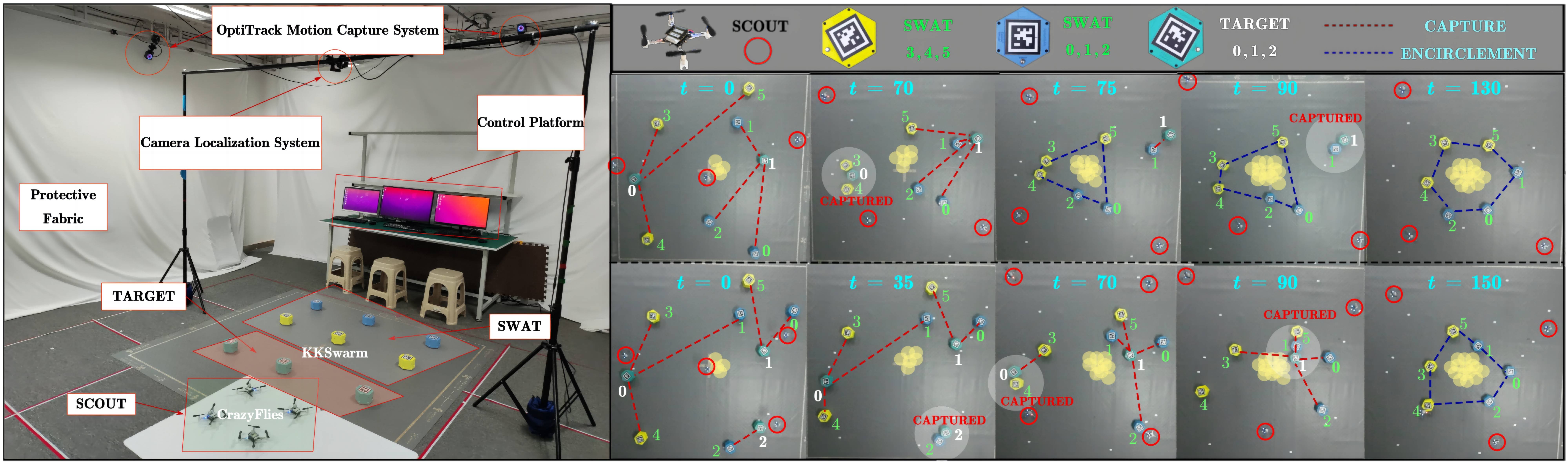
Figure 9: Snapshots of the hardware experiments: experimental setup (left), $11$ robots (right-top) and $13$ robots (right-bottom), where UAVs are SCOUT robots and UGVs are TARGET and SWAT robots.

IV-D Hardware Experiment

Hardware experiments are conducted on a large fleet of UAVs and UGVs, close to the maximum capability of our lab. Detailed descriptions of the setup including state estimation, motion control and software architecture can be found in the supplementary material. Due to the modularization of our system, most existing localization techniques can be integrated to provide state estimation, such as GPS, RTK, UWB and SLAM-based localization. Fig. 9 contains the snapshots where the proposed NAC is applied to two distinct scenarios, i.e., $11$ robots ($6$ SWAT, $2$ TARGET, $3$ SCOUT) and $13$ robots ($6$ SWAT, $3$ TARGET, $4$ SCOUT) with different initial states and distribution of resources.

More specifically, in the first scenario shown in Fig. 9, $3$ SCOUT robots periodically are assigned to perform the exploration tasks in these regions with higher uncertainty. Initially SWAT robots $3,4$ are assigned to TARGET robot $0$ while other SWAT robots move towards TARGET robot $1$. At $t=70s$, TARGET robot $0$ is captured by the proposed collaborative strategy. Afterwards, the SWAT robots $3,4$ switch to the capture task of TARGET robot $1$, while other SWAT robots encircle the resources in the middle. This is because the utility of performing the encirclement task is higher than the capture task of TARGET robot $1$. Once TARGET robot $1$ is finally captured at $t=90s$, all SWAT robots return the encirclement task but with a different topology, until the termination at $t=130s$. In the second scenario shown in Fig. 9, more TARGET robots and SCOUT robots are deployed in differently initial positions. It results in a $98\%$ coverage in $100s$, compared with only $90\%$ in $130s$ for the first scenario. An immediate outcome is that switches of task assignment happen more frequently, during which all tasks are finished at $t=150s$. These results demonstrate that the proposed method can be deployed to rather large-scale robotic fleets. Experiment videos can be found in the supplementary material.

V Conclusion & Future Work

A fully-distributed and generic coalition strategy called KS-COAL is proposed in this work. Different from most centralized approaches, it requires only local communication and ensures a K-serial Stable solution upon termination. Furthermore, HGAN-based heuristics are learned to accelerate KS-COAL during dynamic scenes by selecting more appropriate parameters and promising initial solutions. Practical concerns such as communication delays, motion and perception uncerainties might degrade the effectiveness of the method, which is part of our ongoing investigation. Future work involves (i) the consideration of temporal constraints between collaborative tasks such as precedence and concurrency, which requires more long-term planning; (ii) the learning and prediction of adversarial behaviors for large-scale games.

References

- [1] A. Khan, B. Rinner, and A. Cavallaro, “Cooperative robots to observe moving targets,” IEEE Transactions on Cybernetics, vol. 48, no. 1, pp. 187–198, 2016.
- [2] R. S. De Moraes and E. P. De Freitas, “Multi-uav based crowd monitoring system,” IEEE Transactions on Aerospace and Electronic Systems, vol. 56, no. 2, pp. 1332–1345, 2019.
- [3] T. H. Chung, G. A. Hollinger, and V. Isler, “Search and pursuit-evasion in mobile robotics,” Autonomous Robots, vol. 31, no. 4, pp. 299–316, 2011.
- [4] I. E. Weintraub, M. Pachter, and E. Garcia, “An introduction to pursuit-evasion differential games,” in American Control Conference (ACC). IEEE, 2020, pp. 1049–1066.
- [5] T. Michalak, T. Rahwan, E. Elkind, M. Wooldridge, and N. R. Jennings, “A hybrid exact algorithm for complete set partitioning,” Artificial Intelligence, vol. 230, pp. 14–50, 2016.
- [6] T. Rahwan, T. P. Michalak, M. Wooldridge, and N. R. Jennings, “Coalition structure generation: A survey,” Artificial Intelligence, vol. 229, pp. 139–174, 2015.
- [7] Q. Li, M. Li, B. Q. Vo, and R. Kowalczyk, “An anytime algorithm for large-scale heterogeneous task allocation,” in International Conference on Engineering of Complex Computer Systems (ICECCS), 2020, pp. 206–215.
- [8] F. M. Delle Fave, A. Rogers, Z. Xu, S. Sukkarieh, and N. R. Jennings, “Deploying the max-sum algorithm for decentralised coordination and task allocation of unmanned aerial vehicles for live aerial imagery collection,” in IEEE International Conference on Robotics and Automation (ICRA), 2012, pp. 469–476.
- [9] F. Präntare and F. Heintz, “An anytime algorithm for optimal simultaneous coalition structure generation and assignment,” Autonomous Agents and Multi-Agent Systems, vol. 34, no. 1, pp. 1–31, 2020.
- [10] T. Olsen, A. M. Tumlin, N. M. Stiffler, and J. M. O’Kane, “A visibility roadmap sampling approach for a multi-robot visibility-based pursuit-evasion problem,” in IEEE International Conference on Robotics and Automation (ICRA), 2021, pp. 7957–7964.
- [11] J. Paulos, S. W. Chen, D. Shishika, and V. Kumar, “Decentralization of multiagent policies by learning what to communicate,” in International Conference on Robotics and Automation (ICRA), 2019, pp. 7990–7996.
- [12] E. Garcia, D. W. Casbeer, A. Von Moll, and M. Pachter, “Multiple pursuer multiple evader differential games,” IEEE Transactions on Automatic Control, vol. 66, no. 5, pp. 2345–2350, 2020.
- [13] V. G. Lopez, F. L. Lewis, Y. Wan, E. N. Sanchez, and L. Fan, “Solutions for multiagent pursuit-evasion games on communication graphs: Finite-time capture and asymptotic behaviors,” IEEE Transactions on Automatic Control, vol. 65, no. 5, pp. 1911–1923, 2019.
- [14] V. S. Chipade and D. Panagou, “Multiagent planning and control for swarm herding in 2-d obstacle environments under bounded inputs,” IEEE Transactions on Robotics, vol. 37, no. 6, pp. 1956–1972, 2021.
- [15] X. Fang, C. Wang, L. Xie, and J. Chen, “Cooperative pursuit with multi-pursuer and one faster free-moving evader,” IEEE transactions on cybernetics, 2020.
- [16] A. Torreño, E. Onaindia, A. Komenda, and M. Štolba, “Cooperative multi-agent planning: A survey,” ACM Computing Surveys (CSUR), vol. 50, no. 6, pp. 1–32, 2017.
- [17] M. Gini, “Multi-robot allocation of tasks with temporal and ordering constraints,” in AAAI Conference on Artificial Intelligence, 2017.
- [18] R. Jonker and T. Volgenant, “Improving the hungarian assignment algorithm,” Operations Research Letters, vol. 5, no. 4, pp. 171–175, 1986.
- [19] R. Massin, C. J. Le Martret, and P. Ciblat, “A coalition formation game for distributed node clustering in mobile ad hoc networks,” IEEE Transactions on Wireless Communications, vol. 16, no. 6, pp. 3940–3952, 2017.
- [20] R. Fukasawa, H. Longo, J. Lysgaard, M. P. De Aragão, M. Reis, E. Uchoa, and R. F. Werneck, “Robust branch-and-cut-and-price for the capacitated vehicle routing problem,” Mathematical programming, vol. 106, no. 3, pp. 491–511, 2006.
- [21] L. Vig and J. A. Adams, “Multi-robot coalition formation,” IEEE Transactions on Robotics, vol. 22, no. 4, pp. 637–649, 2006.
- [22] C. De Souza, R. Newbury, A. Cosgun, P. Castillo, B. Vidolov, and D. Kulić, “Decentralized multi-agent pursuit using deep reinforcement learning,” IEEE Robotics and Automation Letters, vol. 6, no. 3, pp. 4552–4559, 2021.
- [23] L. Zhou, V. D. Sharma, Q. Li, A. Prorok, A. Ribeiro, P. Tokekar, and V. Kumar, “Graph neural networks for decentralized multi-robot target tracking,” in IEEE International Symposium on Safety, Security, and Rescue Robotics (SSRR), 2022, pp. 195–202.
- [24] X. Wang, H. Ji, C. Shi, B. Wang, Y. Ye, P. Cui, and P. S. Yu, “Heterogeneous graph attention network,” in The World Wide Web Conference, 2019, pp. 2022–2032.
- [25] M. Fey and J. E. Lenssen, “Fast graph representation learning with PyTorch Geometric,” in ICLR Workshop on Representation Learning on Graphs and Manifolds, 2019.
- [26] Q. Li, “Task allocation and team formation in large-scale heterogeneous multi-agent systems,” Ph.D. dissertation, Swinburne University Of Technology, 2022.