The Impact of Anisotropy on Neutron Star Properties: Insights from -- Universal Relations
Abstract
Anisotropy in pressure within a star emerges from exotic internal processes. In this study, we incorporate pressure anisotropy using the Quasi-Local model. Macroscopic properties, including mass (), radius (), compactness (), dimensionless tidal deformability (), the moment of inertia (), and oscillation frequency (), are explored for the anisotropic neutron star. Magnitudes of these properties are notably influenced by anisotropy degree. Universal -- relations for anisotropic stars are explored in this study. The analysis encompasses various EOS types, spanning from relativistic to non-relativistic regimes. Results show the relation becomes robust for positive anisotropy, weakening with negative anisotropy. The distribution of -mode across - parameter space as obtained with the help of - relation was analyzed for different anisotropic cases. Using tidal deformability data from GW170817 and GW190814 events, a theoretical limit for canonical -mode frequency is established for isotropic and anisotropic neutron stars. For isotropic case, canonical -mode frequency for GW170817 event is ; for GW190814 event, it is . These relationships can serve as reliable tools for constraining nuclear matter EOS when relevant observables are measured.
1 Introduction
The detection of gravitational waves (GWs) is a crucial objective in astrophysics today, with significant efforts being devoted to this problem globally. Several ground-based experiments and space missions have already been devised and are poised to yield significant discoveries in the near future [1, 2, 3, 4, 5]. Furthermore, ongoing efforts are underway to develop a third-generation GW telescope, such as the Einstein Telescope [6] and Cosmic Explorer [7], which promise even higher levels of sensitivity. The reason why the detection of GWs is so challenging is that they are incredibly weak, necessitating detectors with very high sensitivity, as well as the precise waveform of the signal emitted from astrophysical objects.
Neutron stars (NSs) exhibit oscillations that are regarded as potential sources of GWs, manifesting in various forms including radial [8, 9, 10, 11, 12, 13] and non-radial [14, 15, 16, 17] modes. When a NS experiences external or internal disturbances, it emits GWs through different oscillation modes known as quasi-normal modes (QNMs), each characterized by the restoring force that brings them back to their equilibrium state. Notable QNMs include the fundamental mode (-mode) [18, 19, 20], pressure mode (-mode) [21, 15], gravity mode (-mode) [22, 23, 24, 25, 26, 27, 28, 29], rotational mode (-mode) [30, 31, 32, 33, 34, 35], space-time mode (-mode) [36, 37], and other modes [38, 39, 40, 41]. The frequencies of these oscillations are directly linked to the internal structure and composition of the stars [42]. Theoretical studies indicate that the -mode possesses the highest likelihood of being detected initially, with approximately 10% of the gravitational radiation attributed to -mode oscillations for [43].
Different modes of oscillation exhibit distinct behaviors depending on the type of star, offering valuable insights. For instance, the signature of the hadron-quark phase transition can be inferred through the observation of both and -modes in hybrid stars [39]. A study by Flores and Lugones [40] suggests that compact objects emitting GWs within the frequency range of kHz may be hybrid stars, while frequencies exceeding 7 kHz could indicate strange stars. However, the nature of compact objects and their GW emissions still pose challenges due to the limitations of our terrestrial detectors, which are unable to detect certain frequency ranges. Nonetheless, constraints on the frequency of various modes can be established by establishing relationships between the frequency and specific properties of NSs. Several approaches have been proposed to link the -mode frequency with various NS properties, including compactness [44], the moment of inertia [45], and tidal deformability [46, 47, 48]. In this work, we aim to derive such relationships in a model-independent manner, known as universal relations (URs). These URs provide valuable insights into the properties of NSs and their associated oscillation modes.
In literature, there are several URs have already been established between different properties of the NS [49, 50, 51, 52, 53, 54, 55, 56, 57, 58, 59]. However, the focus of this study primarily lies on the relations specifically for anisotropic NSs. Previous URs proposed thus far have mainly been formulated for isotropic NSs, assuming a matter-energy distribution characterized by an isotropic perfect fluid. However, at extremely high-density regions, the presence of nuclear matter can induce deviations between the tangential and radial components of pressure, leading to the emergence of an anisotropic fluid. To obtain more accurate results, we aim to include the effects of anisotropy in our analysis. Anisotropy in NSs can arise from various factors, such as the influence of a high magnetic field [60, 61, 62, 63, 64, 65, 66, 67], pion condensation [68], phase transitions [69], relativistic nuclear interactions [70, 71], core crystallization [72], and the presence of superfluid cores [73, 74, 75], among others. Several models have been proposed to incorporate anisotropy within NSs, such as the Bowers-Liang model [76], Horvat et al. model [77], Cosenza et al. model [78], and others. In this study, we will primarily focus on the Quasi-Local (QL) model, as proposed by Horvat et al. [77], to describe anisotropy within NSs. More details about the QL-model will be elaborated in Section 2.2.
The presence of pressure anisotropy within NSs has a significant impact on various macroscopic properties, including the mass-radius relation, compactness, surface redshift, moment of inertia, tidal deformability, and non-radial oscillations [79, 80, 81, 82, 83, 84, 85, 86, 87, 88, 89, 90, 91, 92, 93, 94, 95, 96, 79]. The specific impact on these quantities varies depending on the degree of anisotropy and the choice of the model employed. Biswas and Bose constrained the degree of anisotropy within stars utilizing tidal deformability data from the GW170817 event [92]. More recently, the Love universal relation for anisotropic NSs has been proposed. By incorporating observational data from GW170817, constraints have been placed on the moment of inertia and radius of canonical anisotropic stars for different degrees of anisotropy [97].
In this study, we introduce the URs for anisotropic NSs for the first time, utilizing a range of models describing unified EOSs such as RMF models (for npe, hyperonic npeY, and strange npeYs matter), density-dependent RMF models, and Skyrme-Hartree-Fock (SHF) models [98, 99, 100, 101, 102, 103, 104, 105]. The unified EOSs closely reproduce the properties of finite nuclei, nuclear matter, and NSs and support star. A total of 60 EOSs (35 from RMF models and 25 from SHF models) are considered in this paper. By employing these EOSs, we calculate various macroscopic properties of NSs with varying degrees of anisotropy using the QL-model. The primary objective of this work is to constrain the -mode frequency of anisotropic stars by leveraging recent observational data. Detailed formalism, results, and discussions are presented in the subsequent sections, shedding light on the intricate relationship between anisotropy, macroscopic properties, and the -mode frequency in NSs.
2 Theoretical Framework
2.1 Stellar Structure Equations
The stress-energy tensor corresponds to the anisotropic distribution of matter-energy as follows [85]
| (2.1) |
where represents the four-velocity of the fluid, and is a unit space-like four-vector. In addition, denotes the energy density, and represents the anisotropic pressure (), where and are the tangential and radial pressure respectively. The four-vectors and must fulfill the following conditions .
The stellar structure can be obtained by solving the Tolman-Oppenheimer-Volkoff (TOV) equations for the anisotropic matter-energy distribution as follows [106, 107]
| (2.2) |
where denotes the enclosed mass corresponding to radius , and represents the metric function defined as
In order to numerically solve the aforementioned set of coupled ordinary differential equations (ODEs), specific boundary conditions need to be established. Conventionally, the surface of the star is set at , where the radial pressure becomes zero (). As the equilibrium system exhibits spherical symmetry, the Schwarzschild metric is employed to describe the exterior space-time. This choice ensures metric continuity at the surface of the anisotropic neutron star (NS) and imposes a boundary condition on . Specifically, the value of at must coincide with the value of in the Schwarzschild metric at .
By making a selection of an EOS governing the radial pressure () and adopting an anisotropic model for , it becomes feasible to numerically solve Eq. (2.1). This numerical solution involves specifying a central energy density , while enforcing the initial condition .
2.2 Anisotropy Model
For anisotropic NS, we use the Quasi-Local (QL) model proposed by Horvat et al. [108] describing the quasi-local nature of anisotropy in the following
| (2.3) |
where the factor depicts the measurement of the degree of anisotropy in the fluid and () also known as local compactness is the quasi-local variable. In order to maintain their spherically symmetric configuration, anisotropic NSs must adhere to specific conditions, as outlined in references [85, 109]. These conditions include:
-
•
Absence of anisotropy at the center of the NS i.e. , or equivalently, at .
-
•
Positivity of and throughout the entire star.
-
•
Positivity of the null energy density , dominant energy density , and strong energy density within the star.
-
•
Non-negativity of the sound speed () inside the star, with the in the radial and tangential directions satisfying the following constraints: . It is also essential to ensure that the speed of sound does not exceed the speed of light ( in this study).
Therefore, the conditions mentioned above are crucial for maintaining the spherical symmetry and physical consistency of anisotropic NSs.
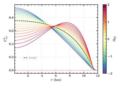
The advantage of using the QL-model with anisotropy is that it ensures the fluid remains isotropic at the center of the star due to the behavior of when , while also being applicable only to relativistic configurations where anisotropy may arise at high densities [91]. For the 60 EOS-ensembles considered in this study, the QL-model with anisotropy parameter ranging from satisfies all the necessary conditions to maintain spherical symmetry in an anisotropic NS configuration [85, 109]. Fig. 1 shows that the speed of sound in the tangential direction () for maximum mass configuration corresponds to DD2 EOS, satisfies the causality condition throughout the star for .
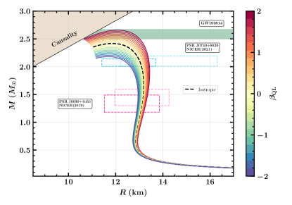
The mass-radius (MR) profile for a given EOS can be obtained by solving the TOV Eqs. (2.1) for various central densities, which generate a sequence of mass and radius. Figure 2 illustrates the MR profiles for the anisotropic star for the DD2 EOS. Adjusting the value of influences the maximum mass and the corresponding radius of the NS. The positive value of increases the maximum mass and its associated radius, and vice-versa for . Observational data from different observations, such as X-ray, NICER, and GW (GW170817 and GW190814), to constrain the degree of anisotropy within NS [110, 111, 112, 113, 114]. For example, values of satisfy the mass constraint (2.50–2.67 ) of the GW190814 event, suggesting that one of the merger companions may have been a highly anisotropic NS [83].
2.3 Slowly Rotating NS and Moment of Inertia
The MI of a slowly rotating anisotropic NS can be expressed as [88, 97]
| (2.4) |
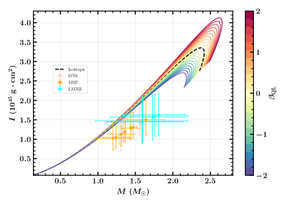
The MI of an anisotropic NS is shown as a function of its mass in the left panel of Fig. 2. As the NS mass increases, the MI also increases until a stable configuration is reached, after which it starts to decrease. Furthermore, both the mass and MI of the NS increase with positive values of , while the opposite trend is observed for negative values of . The impact of anisotropy on the MI is more pronounced for high-mass NSs compared to low-mass ones. Kumar and Landry [99] have established constraints on the MI inferred from various sources such as double neutron stars (DNS), millisecond pulsars (MSP), and low-mass X-ray binaries (LMXB). The error bars in the figure represent the possible range of values for these constraints.
2.4 Tidal Deformability Parameters
When the NS is present in the external field () created by its companion star, it acquires a quadrupole moment (). The magnitude of the quadrupole moment is linearly proportional to the tidal field and is given by [115, 116]
| (2.5) |
where is the tidal deformability of a star. can be defined in terms of tidal Love number as . The dimensionless tidal deformability of the star is defined as . The detailed derivation of for an anisotropic star can be found in Ref. [92, 97, 109].
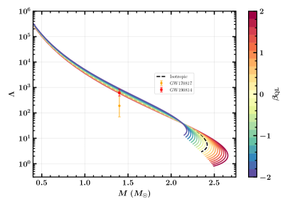
The dimensionless tidal deformability of anisotropic NSs is shown in Figure 3. As the anisotropy parameter increases, the magnitude of the Love number and its corresponding tidal deformability decrease, while they increase with decreasing . The impact of anisotropy on tidal deformability, as mentioned above, reverses after attaining maximum mass configuration, beyond which the star becomes unstable. The GW170817 [113] event constrains to be , while GW190814 [114] put a limit of (in the NS-BH scenario). The predicted value of satisfies the GW190814 limit for almost all values of , whereas, for DD2 EOS, the GW170817 limit is met in the range of . However, sharply decreases once the stable configuration is exceeded.
2.5 Non-Radial Oscillation in Cowling approximation
The Cowling approximation, initially proposed by Cowling [117] for Newtonian stars and later extended to the case of NSs by McDermott et al. [14]. Under this approximation, the metric perturbations are neglected, keeping the space-time metric fixed. We will provide a brief explanation of the derivation of the perturbation equations in the Cowling formalism in the following, while more comprehensive details can be found in [81]. One can obtain the oscillation equations in the Cowling approximation by considering a harmonic time dependence for the perturbation function and , where represents the oscillation frequency in the following [81, 118]
| (2.6) | ||||
To solve the equations mentioned earlier, it is necessary to consider boundary conditions at the center and surface of the star in the following
| (2.7) |
and the boundary condition at the star center satisfies
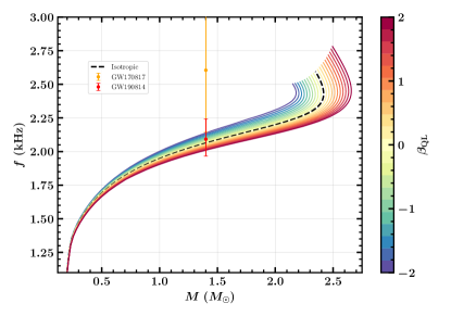
where, the functions and are defined as and . In this work, we focus on the quadrupolar modes, which correspond to . In Fig. 3, we show the -mode frequency of a NS as a function of its mass by varying the anisotropic parameter for the DD2 EOS as a representative case. For a specific mass NS, the frequency decreases for a positive value of while increases for a negative till maximum mass is attained, after which the star becomes unstable. Using the tidal deformability limit from GW170817 and GW190814, one can impose constraints on the canonical -mode frequency for isotropic and anisotropic stars, as discussed in sub-sec. 3.4. We also overlaid the derived theoretical limit on the figure to assess its consistency.
3 Universal Relations
The main purpose of UR is to explore the star properties that are difficult to measure through observations. Several URs have already been proposed to estimate the properties of NS, but they are primarily focused on isotropic cases [119, 51, 120, 121, 49, 122]. However, very few studies have been dedicated to URs for anisotropic stars, which are more realistic than isotropic ones. Hence, in this study, we aim to explore various types of URs between the moment of inertia, tidal deformability, compactness, and -mode frequency for anisotropic NSs.
Although some known URs for anisotropic NS have been proposed in Refs. [50, 92, 97], our primary focus will be on the URs between the moment of inertia, -mode frequency, and compactness (--) as well as the -Love relation of the anisotropic NS. The NS oscillate with different modes, emitting gravitational waves (GWs). The oscillation frequencies, such as the -mode , -mode, etc., might be detectable in the near future with our terrestrial detectors. However, to interpret these observations effectively, we require prior theoretical knowledge. Therefore, approximate URs for anisotropic NSs hold great significance in astrophysical observations.
Before delving into different URs, it is necessary to normalize/dimensionless certain key parameters of NSs that are required to obtain the URs. In this study, we have used the unit of MI and frequency of the -mode as kgm3 and Hz, respectively. Therefore, these quantities need to be normalized, and their normalized values are given as
-
•
Normalised MI (
-
•
Normalised -mode frequency (
Here, we calculate the URs between -, -, -, and -Love for anisotropic NSs. For this study, we chose 60 EOSs, as mentioned in the introduction. Regarding anisotropy, we adopt the same QL-model with different degrees of anisotropy, varying from to . Alternatively, one may opt for other models, such as Bower-Liang’s, as used in Ref. [97].
3.1 - relation
The - UR for isotropic NS with a few EOSs was first calculated by Lau et al. [45]. Breu and Rezzolla [51] studied the universal behavior of dimensionless MI, which is defined as , and is more accurate than the dimensionless MI defined earlier, . Lau and Leung replaced with , called as normalized MI/effective compactness, due to its proportionality with compactness for stars. Therefore, in this study, we use rather than . The relation between - for anisotropic NSs is performed using the least-squares fit with the approximate formula
| (3.1) |
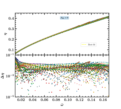
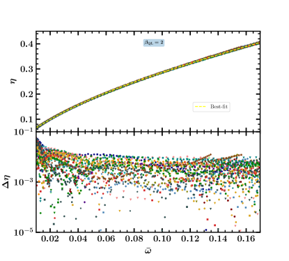
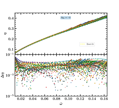
The normalized MI () is plotted as the function of normalized -mode frequency () in Figs. 4-5 with for anisotropic NS. The residuals are computed with the formula,
| (3.2) |
We enumerated the coefficients () with their corresponding reduced chi-squared () errors in Table 1. An increase in anisotropy results in a decrease in the value of error, indicating stronger EOS insensitive relation, and vice versa.
3.2 - relation
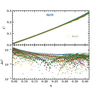
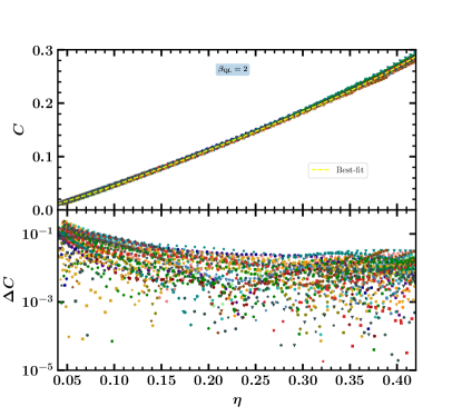
Andersson and Kokkotas [38] first established the correlation between and -mode frequency. Here, we calculate the - relations for anisotropic NSs, using the approximate formula obtained through least-squares fitting
| (3.3) |
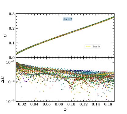
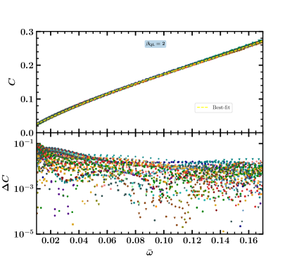
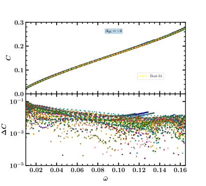
Compactness is plotted as the function of normalized -mode frequency () in Figs. 6-7 with for anisotropic NS. The coefficients () with error are enumerated in Table 1. The magnitude of increases with increasing , implying that the fitting is more robust for the isotropic case. Additionally, also increases with the inclusion of anisotropy, and it is the minimum for the isotropic case. Therefore, the inclusion of anisotropy (whether positive or negative) weakens the EOS insensitive - UR.
| - | |||||
|---|---|---|---|---|---|
| -2.0 | -1.0 | 0.0 | +1.0 | +2.0 | |
| 2.825 | 2.848 | 2.918 | 2.886 | 2.903 | |
| 3.945 | 3.919 | 3.865 | 3.874 | 3.856 | |
| -2.436 | -2.303 | -2.139 | -2.092 | -2.011 | |
| 1.364 | 1.218 | 1.059 | 0.982 | 0.889 | |
| -2.852 | -2.457 | -2.064 | -1.852 | -1.613 | |
| 13.511 | 8.514 | 5.338 | 3.541 | 2.517 | |
| - | |||||
|---|---|---|---|---|---|
| -2.0 | -1.0 | 0.0 | +1.0 | +2.0 | |
| 4.007 | 4.093 | 4.084 | 4.197 | 4.249 | |
| 2.232 | 2.220 | 2.223 | 2.212 | 2.209 | |
| -8.752 | -8.143 | -7.963 | -7.531 | -7.269 | |
| 3.066 | 2.656 | 2.629 | 2.371 | 2.211 | |
| 4.836 | 6.740 | -3.179 | 5.173 | -7.423 | |
| 2.228 | 1.702 | 1.846 | 2.282 | 2.871 | |
| - | |||||
|---|---|---|---|---|---|
| -2.0 | -1.0 | 0.0 | +1.0 | +2.0 | |
| -8.651 | -8.244 | -8.941 | -7.860 | -7.637 | |
| 4.473 | 4.348 | 4.477 | 4.236 | 4.171 | |
| 1.360 | 1.465 | 1.389 | 1.557 | 1.612 | |
| -3.986 | -4.288 | -4.080 | -4.516 | -4.668 | |
| 4.892 | 5.272 | 5.147 | 5.610 | 5.827 | |
| 6.338 | 6.382 | 6.436 | 6.313 | 6.210 | |
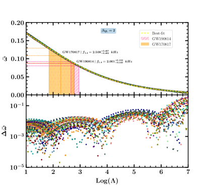
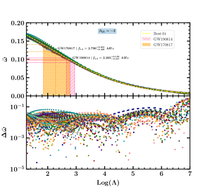
One of the primary applications of - UR involves determining and based on the analysis of observed mode data, as articulated by Andersson and Kokkotas [44]. For a unique choice of -mode frequency the - UR can be exploited to construct a - relation. This constrained relationship, accounting for uncertainties represented by standard deviations in UR, yields - bands, illustrated in the left panel of Fig. 8. In this representation, the orange - band delineates a region where neutron stars are anticipated to exhibit a frequency of kHz, with the solid dashed line denoting kHz. Similarly, the pink band corresponds to a region where neutron stars are expected to possess a frequency of kHz, and the solid dashed line represents kHz. It is noteworthy that the frequency constraints employed for plotting - bands align with the canonical -mode frequency constraints for isotropic neutron stars determined in this study for the GW170817 and GW190814 events. The horizontal error bars in the left panel of Fig. 8 indicate radius limits imposed by the - bands of the respective events, considering a canonical mass neutron star.
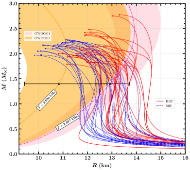
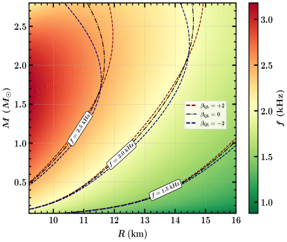
The right panel of Fig. 8 portrays the distribution of -mode frequencies across the - parameter space for isotropic neutron stars based on - UR. The black dashed line represents a specific set of mass and radius values for isotropic stars, anticipated to exhibit the mentioned frequency according to - UR. The figure also depicts variations in these - lines resulting from the inclusion of anisotropy. NSs with frequencies kHz lie in the low compactness region and suffer minimal changes in mass and radius due to the inclusion of anisotropy. Through observing - lines as depicted in Fig. 8, we can conclude that for a constant mass NS having a fixed frequency with kHz, the radius would tend to decrease with the presence of positive anisotropy and increase for negative anisotropy, altering the compactness of the star in order to maintain its natural frequency till a certain critical point/set of mass and radius is reached. After this, the effect of anisotropy on - lines reverses. This kind of behavior in which my effects of anisotropy on the NS parameter reverses occurs due to the presence of an unstable core which suggests us that the critical mass-radius point in the - curves is the maximum stability point, beyond which the NSs are unstable in nature.

3.3 - relation
The relationship between the dimensionless MI () and compactness has been established as a lower-order polynomial fit by Ravenhall and Pethick [123]. Since then, this relation has been studied and modified by various authors, including for the double pulsar system with higher-order polynomial fitting [124], scalar-tensor theory and gravity [122, 125], rotating stars [51], and strange stars [126]. In this work, we investigate the - relations for anisotropic NS using the normalized moment of inertia () instead of the dimensionless one. We use the approximate formula to perform a least-squares fit
| (3.4) |
We display the relationship between and for anisotropic NSs with , respectively in Figs. 9-10. We observe that the inclusion of anisotropy has little effect on the error, indicating that the - UR is conserved even when anisotropy is present, especially for NSs with low compactness.
3.4 -Love relation
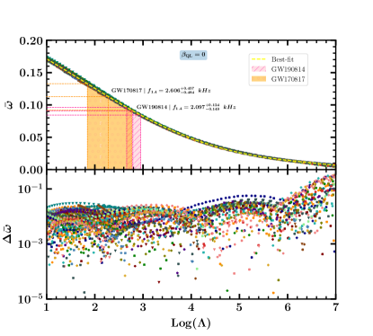
An important tool for studying the oscillation of NSs through observational exploration is a UR between the non-radial -mode frequency (a promising source of GWs) and the tidal deformability (a parameter that can be extracted from the GW data). The exploration of multi-polar universal relations between the -mode frequency and tidal deformability of compact stars was first explored by Chan et al. [46] and further improvised by Pradhan et al. [48]. Recently, Sotani and Kumar [47] introduced a UR between the quasi-normal modes and tidal deformability for isotropic NSs. In this work, we calculate the -Love relations for anisotropic NSs and perform a least-squares fit using the approximate formula
| (3.5) |
The coefficients () with errors are listed in Table 3. For positive values of anisotropy, the errors in decrease, indicating that the EOS-insensitive relations become stronger with the addition of anisotropy. Conversely, for negative values, the errors increase. Therefore, positive values of anisotropy strengthen the -Love UR.
| -2.0 | -1.0 | 0.0 | 1.0 | +2.0 | |
|---|---|---|---|---|---|
| 2.001 | 2.037 | 2.077 | 2.131 | 2.169 | |
| -0.964 | -1.998 | -2.722 | -3.607 | -4.158 | |
| -1.857 | -1.443 | -1.215 | -0.874 | -0.699 | |
| 3.795 | 3.207 | 2.975 | 2.406 | 2.260 | |
| -2.155 | -1.873 | -1.815 | -1.538 | -1.464 | |
| 4.149 | 2.311 | 1.269 | 0.917 | 0.735 |
| -2.0 | |||||
|---|---|---|---|---|---|
| -1.0 | |||||
| 0.0 | |||||
| +1.0 | |||||
| +2.0 | |||||
3.5 Comparison Study
We constrain the canonical -mode frequency for GW170817 [113] and GW190814 [114] events across different degrees of anisotropy, as outlined in Table 3. The canonical -mode frequency is also compared with previous studies, focusing on isotropic NS, as listed in Table 4. Notably, the -mode frequency obtained in this study is approximately 30-35% more than the findings of Chan et al. [46], Pradhan et al. [48], and Sotani and Kumar [47]. This difference in the f-mode was anticipated, given that the aforementioned authors employed a full-GR formalism for their -mode calculations, in contrast to our use of the Cowling approximation in this study.
4 Conclusion
In this study, we have explored the properties of anisotropic NS with the help of the QL-model proposed by Horvat et al. [77]. The main motivation for taking the QL-model is that it ensures that , the anisotropy must vanish, and in other parts of the star, the anisotropy must be there. Different fluid conditions are also studied for varieties of EOSs, and it found that all conditions are perfectly satisfied for the QL model. The speed of sound is also non-negative with any degree of anisotropicity for the QL-model in comparison to the BL-model, as mentioned in Refs. [92, 97]. Therefore, one can vary the limit of the QL-model from negative to positive values to calculate various properties of the NS.
Different macroscopic properties of the star have been calculated with different degrees of anisotropy with the help of a variety EOSs spanning from relativistic to non-relativistic cases. It has been observed that the magnitude of the macroscopic properties increases (decreases) for positive (negative) values of . Almost all the considered EOSs satisfy the different observational limits provided by different observations such as X-ray, pulsar, NICER, GWs, etc. One can impose strong constraints on them with the help of these observational data. Furthermore, we found that positive and negative anisotropy affects tidal deformability parameters and quadrupolar non-radial -mode frequency significantly, which suggests that the star with higher anisotropy sustains more life in the inspiral-merger phase, while the star with lower anisotropy is more likely to collapse.
In addition, we have studied the UR for anisotropic NSs for five values of , and . This analysis considered almost 60 tabulated EOS-ensembles spanning a wide range of stiffness, complying with multimessenger constraints. Moreover, one can use the universal relation for anisotropic stars to extract information about different properties that are not directly observable with current detectors and telescopes. By varying the anisotropy value, we calculated the -, -, and - universal relations and fitted them with the polynomial equation using the least-square method. Our results showed that the reduced chi-square errors for the and - relations were , and , respectively, for isotropic stars. In addition to the universal relations, we calculated the -Love universal relation to constrain the canonical -mode frequency for anisotropic stars. We observed that the sensitivity of the - universal relation is weaker for anisotropic stars in comparison to the isotropic case. However, the relation between - and -Love became stronger with increasing anisotropy. The - relation barely changed with the inclusion of anisotropy compared to the other universal relations. The distribution of -mode across mass-radius parameter space of NSs as obtained by utilizing the - relation studied for different anisotropic cases.
With the help of various observational data for dimensionless tidal deformability, such as GW170817 and GW190814, we established a theoretical constraint on the canonical -mode frequency for both isotropic and anisotropic stars, which is presented in Table 3. As our main objective in this paper was to analyze variations in URs resulting from the inclusion of anisotropy, we adhered to the Cowling approximation formalism for computing the -mode. This choice was necessitated by the absence of a comprehensive and reliable full GR formalism for determining QNM in anisotropic NSs. Consequently, for compensation, we calculated constraints on the canonical -mode frequency for isotropic stars, relying on URs obtained by researchers in Ref. [46, 48, 127], which followed a full-GR formalism, and summarized the outcomes in Table 4. This constraint can be refined by incorporating different anisotropy models and considering various phenomena such as magnetic fields, quarks in the core, and dark matter in detail in future work. Therefore, our findings provide avenues for investigating the various mechanisms that generate anisotropy within compact stars and for constraining its degree with observational data.
5 Acknowledgments
I would like to thank P. Landry and T. Zhao for their fruitful discussions regarding universal relations and fitting procedures. B.K. acknowledges partial support from the Department of Science and Technology, Government of India, with grant no. CRG/2021/000101.
References
- [1] B.P. Abbott et al., Ligo: the laser interferometer gravitational-wave observatory, Reports on Progress in Physics 72 (2009) 076901.
- [2] G.M. Harry and (forthe LIGO Scientific Collaboration), Advanced ligo: the next generation of gravitational wave detectors, Classical and Quantum Gravity 27 (2010) 084006.
- [3] F. Acernese et al., The virgo status, Classical and Quantum Gravity 23 (2006) S635.
- [4] T. Accadia et al., Calibration and sensitivity of the virgo detector during its second science run, Classical and Quantum Gravity 28 (2010) 025005.
- [5] F. Antonucci et al., From laboratory experiments to lisa pathfinder: achieving lisa geodesic motion, Classical and Quantum Gravity 28 (2011) 094002.
- [6] M. Punturo et al., The third generation of gravitational wave observatories and their science reach, Classical and Quantum Gravity 27 (2010) 084007.
- [7] E.D. Hall, Cosmic explorer: A next-generation ground-based gravitational-wave observatory, Galaxies 10 (2022) .
- [8] S. Chandrasekhar, The Dynamical Instability of Gaseous Masses Approaching the Schwarzschild Limit in General Relativity., apj 140 (1964) 417.
- [9] G. Chanmugam, Radial oscillations of zero-temperature white dwarfs and neutron stars below nuclear densities., apj 217 (1977) 799.
- [10] K.D. Kokkotas and J. Ruoff, Radial oscillations of relativistic stars, Astronomy & Astrophysics 366 (2001) 565.
- [11] P. Routaray, H.C. Das, S. Sen, B. Kumar, G. Panotopoulos and T. Zhao, Radial oscillations of dark matter admixed neutron stars, Phys. Rev. D 107 (2023) 103039.
- [12] S. Sen, S. Kumar, A. Kunjipurayil, P. Routaray, S. Ghosh, P.J. Kalita et al., Radial oscillations in neutron stars from unified hadronic and quarkyonic equation of states, Galaxies 11 (2023) .
- [13] P. Routaray, A. Quddus, K. Chakravarti and B. Kumar, Probing the impact of WIMP dark matter on universal relations, GW170817 posterior, and radial oscillations, Monthly Notices of the Royal Astronomical Society 525 (2023) 5492 [https://academic.oup.com/mnras/article-pdf/525/4/5492/51554155/stad2628.pdf].
- [14] P.N. McDermott, H.M. van Horn and C.J. Hansen, Nonradial Oscillations of Neutron Stars, ApJ 325 (1988) 725.
- [15] A. Kunjipurayil, T. Zhao, B. Kumar, B.K. Agrawal and M. Prakash, Impact of the equation of state on - and - mode oscillations of neutron stars, Phys. Rev. D 106 (2022) 063005.
- [16] H.C. Das, A. Kumar, S.K. Biswal and S.K. Patra, Impacts of dark matter on the -mode oscillation of hyperon star, Phys. Rev. D 104 (2021) 123006.
- [17] P. Routaray, S.R. Mohanty, H. Das, S. Ghosh, P. Kalita, V. Parmar et al., Investigating dark matter-admixed neutron stars with nitr equation of state in light of psr j0952-0607, Journal of Cosmology and Astroparticle Physics 2023 (2023) 073.
- [18] T. Zhao and J.M. Lattimer, Universal relations for neutron star -mode and -mode oscillations, Phys. Rev. D 106 (2022) 123002.
- [19] B.K. Pradhan and D. Chatterjee, Effect of hyperons on -mode oscillations in neutron stars, Phys. Rev. C 103 (2021) 035810.
- [20] B.K. Pradhan, D. Chatterjee, M. Lanoye and P. Jaikumar, General relativistic treatment of -mode oscillations of hyperonic stars, Phys. Rev. C 106 (2022) 015805.
- [21] H. Sotani and B. Kumar, Universal relations between the quasinormal modes of neutron star and tidal deformability, Phys. Rev. D 104 (2021) 123002.
- [22] L.S. Finn, g-modes in zero-temperature neutron stars, Mon. Not. R. Astron. Soc. 227 (1987) 265.
- [23] A. Reisenegger and P. Goldreich, A New Class of g-Modes in Neutron Stars, ApJ 395 (1992) 240.
- [24] T. Zhao, C. Constantinou, P. Jaikumar and M. Prakash, Quasinormal modes of neutron stars with quarks, Phys. Rev. D 105 (2022) 103025.
- [25] N. Lozano, V. Tran and P. Jaikumar, Temperature Effects on Core g-Modes of Neutron Stars, Galaxies 10 (2022) 79.
- [26] C. Constantinou, S. Han, P. Jaikumar and M. Prakash, g modes of neutron stars with hadron-to-quark crossover transitions, Phys. Rev. D 104 (2021) 123032.
- [27] P. Jaikumar, A. Semposki, M. Prakash and C. Constantinou, g -mode oscillations in hybrid stars: A tale of two sounds, Phys. Rev. D 103 (2021) 123009.
- [28] W. Wei, M. Salinas, T. Klähn, P. Jaikumar and M. Barry, Lifting the Veil on Quark Matter in Compact Stars with Core g-mode Oscillations, Astrophys. J. 904 (2020) 187.
- [29] V. Tran, S. Ghosh, N. Lozano, D. Chatterjee and P. Jaikumar, g-mode Oscillations in Neutron Stars with Hyperons, 12, 2022.
- [30] B. Haskell, K. Glampedakis and N. Andersson, A new mechanism for saturating unstable r modes in neutron stars, Mon. Not. R. Astron. Soc. 441 (2014) 1662.
- [31] B. Haskell, R-modes in neutron stars: Theory and observations, International Journal of Modern Physics E 24 (2015) 1541007.
- [32] O.P. Jyothilakshmi, P.E.S. Krishnan, P. Thakur, V. Sreekanth and T.K. Jha, Hyperon bulk viscosity and r-modes of neutron stars, Mon. Not. R. Astron. Soc. 516 (2022) 3381.
- [33] L.-M. Lin, Numerical study of nonlinear R-modes in neutron stars, Ph.D. thesis, Washington University in Saint Louis, Missouri, Jan., 2004.
- [34] L. Rezzolla, The r-modes Oscillations and Instability: Surprises from Magnetized Neutron Stars, in Recent Developments in General Relativity, pp. 235–248, Springer, Milano (2002), DOI.
- [35] M. Jasiulek and C. Chirenti, -mode frequencies of rapidly and differentially rotating relativistic neutron stars, Phys. Rev. D 95 (2017) 064060.
- [36] O. Benhar, E. Berti and V. Ferrari, The imprint of the equation of state on the axial w-modes of oscillating neutron stars, Mon. Not. R. Astron. Soc. 310 (1999) 797.
- [37] D. Bandyopadhyay and D. Chatterjee, AXIAL W-MODES OF NEUTRON STARS WITH EXOTIC MATTER, WORLD SCIENTIFIC (2012) 949.
- [38] K.D. Kokkotas and B.G. Schmidt, Quasi-normal modes of stars and black holes, Living Reviews in Relativity 2 (1999) 2.
- [39] H. Sotani, N. Yasutake, T. Maruyama et al., Signatures of hadron-quark mixed phase in gravitational waves, Phys. Rev. D 83 (2011) 024014.
- [40] C.V. Flores and G. Lugones, Discriminating hadronic and quark stars through gravitational waves of fluid pulsation modes, Classical and Quantum Gravity 31 (2014) 155002.
- [41] I.F. Ranea-Sandoval, O.M. Guilera, M. Mariani et al., Oscillation modes of hybrid stars within the relativistic cowling approximation, Journal of Cosmology and Astroparticle Physics 2018 (2018) 031.
- [42] T. Zhao, C. Constantinou, P. Jaikumar et al., Quasinormal modes of neutron stars with quarks, Phys. Rev. D 105 (2022) 103025.
- [43] S. Shibagaki, T. Kuroda, K. Kotake et al., A new gravitational-wave signature of low-T/—W— instability in rapidly rotating stellar core collapse, Monthly Notices of the Royal Astronomical Society: Letters 493 (2020) L138.
- [44] N. Andersson and K.D. Kokkotas, Towards gravitational wave asteroseismology, Monthly Notices of the Royal Astronomical Society 299 (1998) 1059.
- [45] H.K. Lau, P.T. Leung and L.M. Lin, Inferring physical parameters of compact stars from their f-mode gravitational wave signals, The Astrophysical Journal 714 (2010) 1234.
- [46] T.K. Chan, Y.-H. Sham, P.T. Leung et al., Multipolar universal relations between -mode frequency and tidal deformability of compact stars, Phys. Rev. D 90 (2014) 124023.
- [47] H. Sotani and B. Kumar, Universal relations between the quasinormal modes of neutron star and tidal deformability, Phys. Rev. D 104 (2021) 123002.
- [48] B.K. Pradhan, A. Vijaykumar and D. Chatterjee, Impact of updated multipole love numbers and -love universal relations in the context of binary neutron stars, Phys. Rev. D 107 (2023) 023010.
- [49] K. Yagi and N. Yunes, I-love-q relations in neutron stars and their applications to astrophysics, gravitational waves, and fundamental physics, Phys. Rev. D 88 (2013) 023009.
- [50] K. Yagi and N. Yunes, I-love-q anisotropically: Universal relations for compact stars with scalar pressure anisotropy, Phys. Rev. D 91 (2015) 123008.
- [51] C. Breu and L. Rezzolla, Maximum mass, moment of inertia and compactness of relativistic stars, Monthly Notices of the Royal Astronomical Society 459 (2016) 646.
- [52] L. Rezzolla, P. Pizzochero, D. Jones, N. Rea and I. Vidaña, The Physics and Astrophysics of Neutron Stars, Astrophysics and Space Science Library, Springer International Publishing (2019).
- [53] R. Riahi, S.Z. Kalantari and J.A. Rueda, Universal relations for the keplerian sequence of rotating neutron stars, Phys. Rev. D 99 (2019) 043004.
- [54] T. Gupta, B. Majumder, K. Yagi et al., I-love-q relations for neutron stars in dynamical chern simons gravity, Classical and Quantum Gravity 35 (2017) 025009.
- [55] J.-L. Jiang, S.-P. Tang, Y.-Z. Wang et al., Psr j0030+0451, gw170817, and the nuclear data: Joint constraints on equation of state and bulk properties of neutron stars, The Astrophysical Journal 892 (2020) 55.
- [56] C.-H. Yeung, L.-M. Lin, N. Andersson et al., The i-love-q relations for superfluid neutron stars, Universe 7 (2021) .
- [57] S. Chakrabarti, T. Delsate, N. Gürlebeck et al., relation for rapidly rotating neutron stars, Phys. Rev. Lett. 112 (2014) 201102.
- [58] B. Haskell, R. Ciolfi, F. Pannarale et al., On the universality of I–Love–Q relations in magnetized neutron stars, Monthly Notices of the Royal Astronomical Society: Letters 438 (2013) L71.
- [59] D. Bandyopadhyay, S.A. Bhat, P. Char et al., Moment of inertia, quadrupole moment, love number of neutron star and their relations with strange-matter equations of state, The European Physical Journal A 54 (2018) 26.
- [60] S.S. Yazadjiev, Relativistic models of magnetars: Nonperturbative analytical approach, Phys. Rev. D 85 (2012) 044030.
- [61] C.Y. Cardall, M. Prakash and J.M. Lattimer, Effects of strong magnetic fields on neutron star structure, The Astrophysical Journal 554 (2001) 322.
- [62] K. Ioka and M. Sasaki, Relativistic stars with poloidal and toroidal magnetic fields and meridional flow, The Astrophysical Journal 600 (2004) 296.
- [63] R. Ciolfi and L. Rezzolla, Twisted-torus configurations with large toroidal magnetic fields in relativistic stars, Monthly Notices of the Royal Astronomical Society: Letters 435 (2013) L43.
- [64] R. Ciolfi, V. Ferrari and L. Gualtieri, Structure and deformations of strongly magnetized neutron stars with twisted-torus configurations, Monthly Notices of the Royal Astronomical Society 406 (2010) 2540.
- [65] J. Frieben and L. Rezzolla, Equilibrium models of relativistic stars with a toroidal magnetic field, Monthly Notices of the Royal Astronomical Society 427 (2012) 3406.
- [66] A.G. Pili, N. Bucciantini and L. Del Zanna, Axisymmetric equilibrium models for magnetized neutron stars in General Relativity under the Conformally Flat Condition, Monthly Notices of the Royal Astronomical Society 439 (2014) 3541.
- [67] N. Bucciantini, A.G. Pili and L. Del Zanna, The role of currents distribution in general relativistic equilibria of magnetized neutron stars, Monthly Notices of the Royal Astronomical Society 447 (2015) 3278.
- [68] R.F. Sawyer, Condensed phase in neutron-star matter, Phys. Rev. Lett. 29 (1972) 382.
- [69] B. Carter and D. Langlois, Relativistic models for superconducting-superfluid mixtures, Nuclear Physics B 531 (1998) 478.
- [70] V. Canuto, Equation of state at ultrahigh densities, Annual Review of Astronomy and Astrophysics 12 (1974) 167.
- [71] M. Ruderman, Pulsars: Structure and dynamics, Annual Review of Astronomy and Astrophysics 10 (1972) 427.
- [72] S. Nelmes and B.M.A.G. Piette, Phase transition and anisotropic deformations of neutron star matter, Phys. Rev. D 85 (2012) 123004.
- [73] R. Kippenhahn and A. Weigert, Stellar Structure and Evolution, 1990.
- [74] N.K. Glendenning, Compact stars, 1997.
- [75] H. Heiselberg and M. Hjorth-Jensen, Phases of dense matter in neutron stars, Physics Reports 328 (2000) 237.
- [76] R.L. Bowers and E.P.T. Liang, Anisotropic Spheres in General Relativity, ApJ 188 (1974) 657.
- [77] D. Horvat, S. Ilijić and A. Marunović, Radial pulsations and stability of anisotropic stars with a quasi-local equation of state, Classical and Quantum Gravity 28 (2010) 025009.
- [78] M. Cosenza, L. Herrera, M. Esculpi et al., Some models of anisotropic spheres in general relativity, Journal of Mathematical Physics 22 (1981) 118.
- [79] H.O. Silva, C.F.B. Macedo, E. Berti et al., Slowly rotating anisotropic neutron stars in general relativity and scalar–tensor theory, Classical and Quantum Gravity 32 (2015) 145008.
- [80] W. Hillebrandt and K.O. Steinmetz, Anisotropic neutron star models: stability against radial and nonradial pulsations., aap 53 (1976) 283.
- [81] D.D. Doneva and S.S. Yazadjiev, Nonradial oscillations of anisotropic neutron stars in the cowling approximation, Phys. Rev. D 85 (2012) 124023.
- [82] S.S. Bayin, Anisotropic fluid spheres in general relativity, Phys. Rev. D 26 (1982) 1262.
- [83] Z. Roupas, Secondary component of gravitational-wave signal gw190814 as an anisotropic neutron star, Astrophysics and Space Science 366 (2021) 9.
- [84] D. Deb, B. Mukhopadhyay and F. Weber, Effects of anisotropy on strongly magnetized neutron and strange quark stars in general relativity, The Astrophysical Journal 922 (2021) 149.
- [85] G. Estevez-Delgado and J. Estevez-Delgado, On the effect of anisotropy on stellar models, The European Physical Journal C 78 (2018) 673.
- [86] M.L. Pattersons and A. Sulaksono, Mass correction and deformation of slowly rotating anisotropic neutron stars based on hartle–thorne formalism, The European Physical Journal C 81 (2021) 698.
- [87] R. Rizaldy, A.R. Alfarasyi, A. Sulaksono et al., Neutron-star deformation due to anisotropic momentum distribution of neutron-star matter, Phys. Rev. C 100 (2019) 055804.
- [88] A. Rahmansyah, A. Sulaksono, A.B. Wahidin et al., Anisotropic neutron stars with hyperons: implication of the recent nuclear matter data and observations of neutron stars, The European Physical Journal C 80 (2020) 769.
- [89] A. Rahmansyah and A. Sulaksono, Recent multimessenger constraints and the anisotropic neutron star, Phys. Rev. C 104 (2021) 065805.
- [90] L. Herrera, J. Ospino and A. Di Prisco, All static spherically symmetric anisotropic solutions of einstein’s equations, Phys. Rev. D 77 (2008) 027502.
- [91] L. Herrera and W. Barreto, General relativistic polytropes for anisotropic matter: The general formalism and applications, Phys. Rev. D 88 (2013) 084022.
- [92] B. Biswas and S. Bose, Tidal deformability of an anisotropic compact star: Implications of gw170817, Phys. Rev. D 99 (2019) 104002.
- [93] S. Das, B.K. Parida, S. Ray et al., Role of anisotropy on the tidal deformability of compact stellar objects, Physical Sciences Forum 2 (2021) .
- [94] Z. Roupas and G.G.L. Nashed, Anisotropic neutron stars modelling: constraints in krori–barua spacetime, The European Physical Journal C 80 (2020) 905.
- [95] A. Sulaksono, Anisotropic pressure and hyperons in neutron stars, International Journal of Modern Physics E 24 (2015) 1550007.
- [96] A.M. Setiawan and A. Sulaksono, Anisotropic neutron stars and perfect fluid’s energy conditions, The European Physical Journal C 79 (2019) 755.
- [97] H.C. Das, relation for an anisotropic neutron star, Phys. Rev. D 106 (2022) 103518.
- [98] M. Fortin, C. Providência, A.R. Raduta et al., Neutron star radii and crusts: Uncertainties and unified equations of state, Phys. Rev. C 94 (2016) 035804.
- [99] B. Kumar and P. Landry, Inferring neutron star properties from gw170817 with universal relations, Phys. Rev. D 99 (2019) 123026.
- [100] P. Landry and B. Kumar, Constraints on the moment of inertia of psr j0737-3039a from gw170817, The Astrophysical Journal Letters 868 (2018) L22.
- [101] A. Kunjipurayil, T. Zhao, B. Kumar et al., Impact of the equation of state on - and - mode oscillations of neutron stars, Phys. Rev. D 106 (2022) 063005.
- [102] T. Malik, N. Alam, M. Fortin et al., Gw170817: Constraining the nuclear matter equation of state from the neutron star tidal deformability, Phys. Rev. C 98 (2018) 035804.
- [103] N. Alam, B.K. Agrawal, M. Fortin et al., Strong correlations of neutron star radii with the slopes of nuclear matter incompressibility and symmetry energy at saturation, Phys. Rev. C 94 (2016) 052801.
- [104] V. Parmar, H.C. Das, A. Kumar et al., Crustal properties of a neutron star within an effective relativistic mean-field model, Phys. Rev. D 105 (2022) 043017.
- [105] V. Parmar, H.C. Das, A. Kumar et al., Pasta properties of the neutron star within effective relativistic mean-field model, Phys. Rev. D 106 (2022) 023031.
- [106] P. Bhar and P. Rej, Compact stellar model in the presence of pressure anisotropy in modified finch skea space–time, Journal of Astrophysics and Astronomy 42 (2021) 74.
- [107] J.R. Oppenheimer and G.M. Volkoff, On massive neutron cores, Phys. Rev. 55 (1939) 374.
- [108] D. Horvat, S. Ilijić and A. Marunović, Radial pulsations and stability of anisotropic stars with a quasi-local equation of state, Classical and Quantum Gravity 28 (2010) 025009.
- [109] A.M. Setiawan and A. Sulaksono, Anisotropic neutron stars and perfect fluid’s energy conditions, The European Physical Journal C 79 (2019) 755.
- [110] M.C. Miller et al., Psr j0030+0451 mass and radius from nicer data and implications for the properties of neutron star matter, The Astrophysical Journal Letters 887 (2019) L24.
- [111] T.E. Riley et al., A nicer view of psr j0030+0451: Millisecond pulsar parameter estimation, The Astrophysical Journal Letters 887 (2019) L21.
- [112] M.C. Miller et al., The radius of psr j0740+6620 from nicer and xmm-newton data, The Astrophysical Journal Letters 918 (2021) L28.
- [113] LIGO Scientific Collaboration and Virgo Collaboration collaboration, Gw170817: Observation of gravitational waves from a binary neutron star inspiral, Phys. Rev. Lett. 119 (2017) 161101.
- [114] R. Abbott, T.D. Abbott, L.S. Collaboration et al., Gw190814: Gravitational waves from the coalescence of a 23 solar mass black hole with a 2.6 solar mass compact object, The Astrophysical Journal Letters 896 (2020) L44.
- [115] T. Hinderer, Tidal love numbers of neutron stars, The Astrophysical Journal 677 (2008) 1216.
- [116] T. Hinderer, Erratum: “tidal love numbers of neutron stars” (2008, apj, 677, 1216), The Astrophysical Journal 697 (2009) 964.
- [117] T.G. Cowling, The Non-radial Oscillations of Polytropic Stars, Monthly Notices of the Royal Astronomical Society 101 (1941) 367.
- [118] E.J.A. Curi, L.B. Castro, C.V. Flores and C.H. Lenzi, Non-radial oscillations and global stellar properties of anisotropic compact stars using realistic equations of state, The European Physical Journal C 82 (2022) 527.
- [119] N. Jiang and K. Yagi, Analytic i-love-c relations for realistic neutron stars, Phys. Rev. D 101 (2020) 124006.
- [120] C. Chirenti, G.H. de Souza and W. Kastaun, Fundamental oscillation modes of neutron stars: Validity of universal relations, Phys. Rev. D 91 (2015) 044034.
- [121] K. Yagi and N. Yunes, I-Love-Q, Science 341 (2013) 365 [1302.4499].
- [122] K.V. Staykov, D.D. Doneva and S.S. Yazadjiev, Moment-of-inertia–compactness universal relations in scalar-tensor theories and gravity, Phys. Rev. D 93 (2016) 084010.
- [123] D.G. Ravenhall and C.J. Pethick, Neutron Star Moments of Inertia, ApJ 424 (1994) 846.
- [124] J.M. Lattimer and B.F. Schutz, Constraining the equation of state with moment of inertia measurements, The Astrophysical Journal 629 (2005) 979.
- [125] D. Popchev, K.V. Staykov, D.D. Doneva et al., Moment of inertia–mass universal relations for neutron stars in scalar-tensor theory with self-interacting massive scalar field, The European Physical Journal C 79 (2019) 178.
- [126] Bejger, M. and Haensel, P., Moments of inertia for neutron and strange stars: Limits derived for the crab pulsar, A&A 396 (2002) 917.
- [127] H. Sotani, K. Tominaga and K.-i. Maeda, Density discontinuity of a neutron star and gravitational waves, Phys. Rev. D 65 (2001) 024010.