Score-Based Multimodal Autoencoders

Abstract

Multimodal Variational Autoencoders (VAEs) represent a promising group of generative models that facilitate the construction of a tractable posterior within the latent space, given multiple modalities. Daunhawer et al. (2022) demonstrate that as the number of modalities increases, the generative quality of each modality declines. In this study, we explore an alternative approach to enhance the generative performance of multimodal VAEs by jointly modeling the latent space of unimodal VAEs using score-based models (SBMs). The role of the SBM is to enforce multimodal coherence by learning the correlation among the latent variables. Consequently, our model combines the superior generative quality of unimodal VAEs with coherent integration across different modalities.

1 Introduction

The real-world data often has multiple modalities such as image, text, and audio, which makes learning from multiple modalities an important task. Multimodal VAEs are a class of multimodal generative models that are able to generate multiple modalities jointly. Learning from multimodal data is inherently more challenging than from unimodal data, as it involves processing multiple data modalities with distinct characteristics.

In order to learn the joint representation of these modalities, previous approaches generally preferred to encode them to latent distribution that governs the data distribution across different modalities. In general, we expect the following properties from a multimodal generative model:

Multiway conditional generation: If we have some modalities present, we should be able to generate the remaining modalities from the present ones (Shi et al., 2019; Wu and Goodman, 2018). Conditioning should not be restricted to some modalities but we should be able to condition any modality to generate any other modality.

Unconditional generation: If we have no modality present to condition on, we should be able to sample from the joint distribution so that the generated modalities are coherent (Shi et al., 2019). Coherence in this case means that the generated modalities represent the same concept that is expressed in the different modalities we have.

Conditional modality gain: If we provide more information to the model via observing more modalities, we should get better performance in the generated missing modalities. In other words, the generation performance should consistently improve as the number of observed (given) modalities increases.

Scalability: The model should scale as the number of total modalities increases, i.e., the generation performance should not drop as we add more data modality. Moreover, model complexity shouldn’t become computationally inefficient when adding more modalities Sutter et al. (2020).

Other properties like joint representation where we want a representation that takes into account the statistics and properties of all the modalities (Srivastava and Salakhutdinov, 2014; Suzuki et al., 2017) can be easily learned from a multimodal model obtaining the above properties. Another property that we have deferred for future work is weak supervision where we make use of multimodal data that aren’t paired together. Weak supervision makes use of multimodal data that are not paired together Wu and Goodman (2018) as it is difficult to always find labeled multimodal data.

Naively using multimodal VAEs by training all combinations of modalities becomes easily intractable as the number of models to be trained increases exponentially. We will need to train $2^{M}-1$ different combinations of models for each subset of the modalities. Since this is not a scalable approach, previous works have proposed different methods of avoiding this by constructing a joint posterior of all the modalities. They do this by modeling the joint posterior over the latent space $\mathbf{z}$: $q(\mathbf{z}|\mathbf{x}_{1:M})$, where $\mathbf{X}_{1:M}$ is the set of modalities. To ensure the tractability of the inference network q, prior works have proposed using a product of experts (Wu and Goodman, 2018), mixture of experts (Shi et al., 2019), or in the generalized form, mixture of the product of experts (MoPoE) (Sutter et al., 2021) are some of the works on multimodal VAEs.

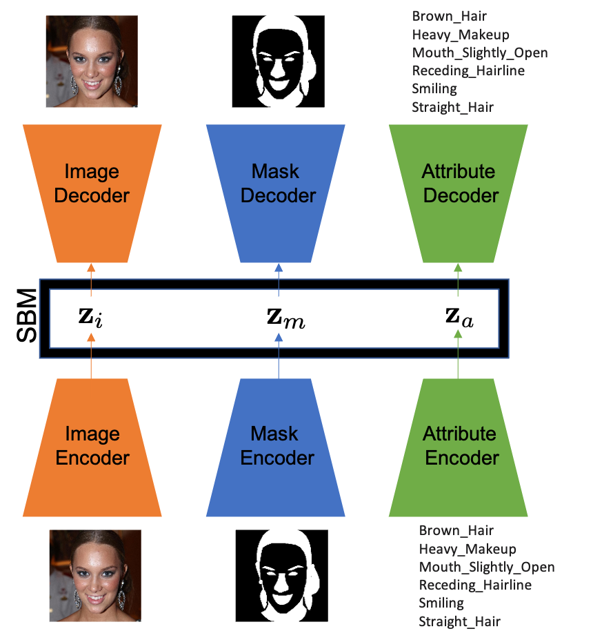
Figure 1: A variational or regularized auto-encoder will be used for each individual modality to get the latent representation which then will be used to train the score-based model which will allow the prediction of any modality given some or none. The auto-encoders are trained independently in the first stage and the respective $z$ of each modality will be used to train the score network.

After selecting on how to fuse the posteriors of different modalities, these approaches then construct the joint multimodal ELBO and use it to train multimodal data. At inference time, they use the modalities that are observed to generate the missing modalities. Wu and Goodman (2018) intentionally adds ELBO subsampling during training to increase the model’s performance on generating missing modalities at inference time. Mixture of experts and mixture of products of experts subsample modalities as part of their training process because of the posterior model is a mixture model. Subsampling of the modalities, as pointed out by  Daunhawer et al. (2022), results in a generative discrepancy among modalities. We also observe that conditioning on more modalities often reduces the quality of the generated modality which goes contrary to one’s expectation. As a model receives additional information, it should perform better and better but this doesn’t happen in previous multimodal VAEs as the generated modalities continue to have lower qualities as more modalities are observed. Daunhawer et al. (2022) further concludes that these models cannot be useful for real-world applications at this point due to these failures.

To overcome these issues, instead of constructing a joint posterior, we try to explicitly model the joint latent space of individual VAEs: $p_{\theta}(\mathbf{z}_{1:M})$. The joint latent model learns the correlation among the individual latent space in a separate score-based model trained independently without constructing a joint posterior as the previous multimodal VAEs. Therefore, it can ensure prediction coherence by sampling from the score model while also maintaining the generative quality that is close to a unimodal VAE. And by doing so, we avoid the need to construct the joint multimodal ELBO. We only use the independently trained unimodal VAEs that will then generate latent samples that will be used to train a score network that will model the joint latent space. This approach is also scalable as it only uses $M$ unimodal VAEs and one score model and it performs better as we condition it on more modalities. That is, as the number of information available increases, the more accurate marginal distribution we get, thus increasing the generative quality. Unconditional generation from the joint distribution can also be done by sampling from the score model respecting the joint distribution. Figure  1 describes the overall architecture of the model.

Our contributions include proposing a novel generative multimodal autoencoder approach that satisfies most of the appealing properties of multimodal VAEs, supported using extensive experimental studies. We also show that our model learns a valid variational lower bound on data likelihood.

2 Methodology

Assuming the each data point consists of $M$ modalities: $\mathbf{x}_{1:M}=(\mathbf{x}_{1},\mathbf{x}_{2},\cdots,\mathbf{x}_{M})$, our latent variable model describes the data distribution as $p(\mathbf{x}_{1:M})=\sum_{\mathbf{z}_{1:M}}p(\mathbf{x}_{1:M}|\mathbf{z}_{1:M})p(\mathbf{z}_{1:M})$, where $\mathbf{z}_{1:M}=(\mathbf{z}_{1},\mathbf{z}_{2},\cdots,\mathbf{z}_{M})$ and $\mathbf{z}_{k}$ is the latent vector corresponding to the $k$th modality. In contrast to common multimodal VAE setups (Wu and Goodman, 2018; Shi et al., 2019), we don’t consider any shared latent representation among different modalities, and we assume each latent variable $\mathbf{z}_{k}$ only captures the modality-specific representation of the corresponding modality $k$. Therefore, the variational lower bound on $\log p(\mathbf{x}_{1:M})$ can be written as:

$$\log p(\mathbf{x}_{1:M}) \geq\mathbb{E}_{q(\mathbf{z}_{1:M}|\mathbf{x}_{1:M})}\log\frac{p(\mathbf{x}_{1:M}|\mathbf{z}_{1:M})p(\mathbf{z}_{1:M})}{q(\mathbf{z}_{1:M}|\mathbf{x}_{1:M})}.$$ (1)

To simplify the joint generative model $p(\mathbf{x}_{1:M}|\mathbf{z}_{1:M})$ and the joint recognition model $q(\mathbf{z}_{1:M}|\mathbf{x}_{1:M})$, we assume two conditional indenpendencies: 1) Given an observed modality $\mathbf{x}_{k}$, its corresponding latent variable $\mathbf{z}_{k}$ is independent of other latent variables, i.e., $\mathbf{x}_{k}$ have enough information to describe $\mathbf{z}_{k}$: $\mathbf{z}_{k}\perp\mathbf{z}_{-k}|\mathbf{x}_{k}$. 2) Knowing the latent variable $\mathbf{z}_{k}$ of $k$th modality is enough to reconstruct that modality: $\mathbf{x}_{k}\perp\mathbf{x}_{-k},\mathbf{z}_{-k}|\mathbf{z}_{k}$. Using these conditional independencies the generative and recognition models factorize as:

$$p(\mathbf{x}_{1:M}|\mathbf{z}_{1:M})=\prod_{k=1}^{M}p(\mathbf{x}_{k}|\mathbf{z}_{k})~{}\text{and}~{}q(\mathbf{z}_{1:M}|\mathbf{x}_{1:M})=\prod_{k=1}^{M}q(\mathbf{z}_{k}|\mathbf{x}_{k}).$$

Therefore we can rewrite the variational lower bound as:

$$\log p(\mathbf{x}_{1:M}) \geq\mathbb{\sum}_{k}E_{q_{\phi_{k}}(\mathbf{z}_{k}|\mathbf{x}_{k})}\log p_{\psi_{k}}(\mathbf{x}_{k}|\mathbf{z}_{k})-D_{\text{KL}}(\prod_{k}q_{\phi_{k}}(\mathbf{z}_{k}|\mathbf{x}_{k})||p_{\theta}(\mathbf{z}_{1:M})),$$ (2)

where $\phi_{k}$ and $\psi_{k}$ are the parameterizations of the recognition and generative models, respectively, and $\theta$ parameterizes the prior. If we assume the prior $p_{\theta}(\mathbf{z}_{1:M})$ factorizes as $\prod_{k}p_{\theta_{k}}(\mathbf{z}_{k})$ then the variational lower bound of $\log p(\mathbf{x}_{1:M})$ become $\sum_{k}\text{ELBO}_{k}$, where $\text{ELBO}_{k}$ is the variational lower bound of individual modality. However, such an assumption ignores the dependencies among latent variables and results in a lack of coherence among generated modalities when using prior for generating multimodal samples. To benefit from the decomposable ELBO but also benefit from the joint prior, we separate the training into two steps. In step I, we maximize the ELBO with respect to $\phi$ and $\psi$ assuming prior $p(\mathbf{z}_{1:M})=\prod\mathcal{N}(\mathbb{0},\sigma\mathbb{I})$, which only regularizes the recognition models. In step II, we optimize ELBO with respect to $\theta$ assuming a joint prior over latent variables. Therefore, in step II maximizing the ELBO reduces to: $\min_{\theta}\text{KL}(\prod_{k}q_{\phi_{k}}(\mathbf{z}_{k}|\mathbf{x}_{k})p_{\theta}(\mathbf{z}_{1:M}))$ and since recognition model is constant w.r.t. $\theta$, the step II becomes $\max_{\theta}\mathbb{E}_{p(\mathbf{x}_{1:M})}\mathbb{E}_{\prod_{k}q(\mathbf{z}_{k}|\mathbf{x}_{k})}\log p_{\theta}(\mathbf{z}_{1:M})$, which is equivalent to maximum likelihood training of the parametric prior using sampled latent variables for each data points. During inference, we only need samples from $p_{\theta}(\mathbf{z}_{1:M})$ thus we can parameterize $s_{\theta}(\mathbf{z}_{1:M})\nabla_{\mathbf{z}_{1:M}}\log(p_{\theta})$ and train the score model $s_{\theta}(\mathbf{z}_{1:M})$ using score matching (Hyvärinen and Dayan, 2005). In practice, score matching objective does not scale to the large dimension which is required in our setup, and other alternatives such as denoising score-matching (Vincent, 2011) and sliced score-matching (Song et al., 2020) have been proposed. Here we use denoising score matching with noise conditional score networks (Song and Ermon, 2019, 2020):

$$\min_{\theta}\frac{1}{L}\sum_{i=1}^{L}\lambda\left(\sigma_{i}\right)\left[\frac{1}{2}\mathbb{E}_{p(\mathbf{x})}\mathbb{E}_{q(\mathbb{z}|\mathbf{x})}\mathbb{E}_{\tilde{\mathbb{z}}\sim\mathcal{N}(\mathbb{z},\sigma_{i}^{2},\mathbb{I})}\bigg{\|}\mathbb{s}_{\theta}(\tilde{\mathbb{z}},\sigma_{i})+\frac{\tilde{\mathbb{z}}-\mathbb{z}}{\sigma_{i}^{2}}\bigg{\|}_{2}^{2}\right].$$ (3)

2.1 Inference with missing modalities

The goal of inference is to sample unobserved modalities (indexed by $\mathbf{u}\subseteq\{1,\cdots,M\}$) given the observed modalities (indexed by $\mathbf{o}\subset\{1,\cdots,M\}$) from $p(\mathbf{x}_{\mathbf{u}}|\mathbf{x}_{\mathbf{o}})$. We define a lower bound on log-probably $\log p(\mathbf{x}_{\mathbf{u}}|\mathbf{x}_{\mathbf{o}})$ using posterior $q(\mathbf{z}_{\mathbf{u}}|\mathbf{z}_{\mathbf{o}},\mathbf{x}_{\mathbf{o}})$ on the latent variables of the unobserved modalities $\mathbf{z}_{\mathbf{u}}$:

$$\log p(\mathbf{x}_{\mathbf{u}}|\mathbf{x}_{\mathbf{o}}) =\log\mathbb{E}_{q(\mathbf{z}_{\mathbf{u}}|\mathbf{z}_{\mathbf{o}},\mathbf{x}_{\mathbf{o}})}p(\mathbf{x}_{\mathbf{u}}|\mathbf{x}_{\mathbf{o}},\mathbf{z}_{\mathbf{u}},\mathbf{z}_{\mathbf{o}})$$

$$\geq\mathbb{E}_{q(\mathbf{z}_{\mathbf{u}}|\mathbf{z}_{\mathbf{o}},\mathbf{x}_{\mathbf{o}})}\log p(\mathbf{x}_{\mathbf{u}}|\mathbf{x}_{\mathbf{o}},\mathbf{z}_{\mathbf{u}},\mathbf{z}_{\mathbf{o}})$$

$$=\mathbb{E}_{q(\mathbf{z}_{\mathbf{u}}|\mathbf{z}_{\mathbf{o}},\mathbf{x}_{\mathbf{o}})}\log p(\mathbf{x}_{\mathbf{u}}|\mathbf{z}_{\mathbf{u}}),$$ (4)

where $p(\mathbf{x}_{\mathbf{u}}|\mathbf{z}_{\mathbf{u}})=\prod_{k\in\mathbf{u}}p_{\psi_{k}}(\mathbf{x}_{k}|\mathbf{z}_{k})$ and $p_{\psi_{k}}(\mathbf{x}_{k}|\mathbf{z}_{k})$ is the generative model for modality $k$. We define the posterior distribution $q(\mathbf{z}_{\mathbf{u}}|\mathbf{z}_{\mathbf{o}},\mathbf{x}_{\mathbf{o}})$ as the following:

$$q(\mathbf{z_{u}}|\mathbf{z_{o}},\mathbf{x_{o}})=\mathbb{\sum}_{\mathbf{z}_{\mathbf{u}}}\left[\prod_{i\in\mathbf{o}}q_{\phi_{i}}(\mathbf{z}_{i}|\mathbf{x}_{i})\right]p_{\theta}(\mathbf{z_{u}}|\mathbf{z_{o}}),$$ (5)

where $q_{\phi_{k}}(\mathbf{z}_{k}|\mathbf{x}_{k})$ is the recognition model for modality $k$.

In order to sample from $p(\mathbf{x}_{\mathbf{u}}|\mathbf{x}_{\mathbf{o}})$, following eq. 5, we first sample $\mathbf{z}_{\mathbf{o}}$ for all observed modalities, and then sample $\mathbf{z}_{\mathbf{u}}$ from $p_{\theta}(\mathbf{z}_{\mathbf{u}}|\mathbf{z}_{\mathbf{o}})$ by setting the latent representation of the observed modalities to $\mathbf{z}_{\mathbf{o}}$ in annealed Langevin dynamics (Welling and Teh, 2011; Song and Ermon, 2020):

$$\mathbb{z_{u}}^{t+1}=\mathbf{z}^{t}_{\mathbf{u}}+\frac{\lambda^{2}}{2}s_{\theta}(\left[\mathbf{z}^{t}_{\mathbf{u}},\mathbf{z_{o}}\right],\sigma^{t})+\lambda\mathcal{N}(\mathbb{0},\mathbb{I}).$$ (6)

After running the Langevin dynamics for $T$ step we use the generative models $p(\mathbf{x}_{\mathbf{u}}|\mathbf{z}_{\mathbf{u}})=\prod_{k\in\mathbf{u}}p_{\psi_{k}}(\mathbf{x}_{k}|\mathbf{z}_{k})$ to sample the unobserved modalities.

3 Related Works

Our work is heavily inspired by earlier works on deep multimodal learning (Ngiam et al., 2011; Srivastava and Salakhutdinov, 2014). Ngiam et al. (2011) use a set of autoencoders for each modality and a shared representation across different modalities and trained the parameters to reconstruct the missing modalities given the present one. Srivastava and Salakhutdinov (2014) define deep Boltzmann machine to represent multimodal data with modality-specific hidden layers followed by shared hidden layers across multiple modalities, and use Gibbs sampling to recover missing modalities.

Suzuki et al. (2017) approached this problem by maximizing the joint ELBO and additional KL terms between the posterior of the joint and the individuals to handle missing data. Tsai et al. (2019) propose a factorized model in a supervised setting over model-specific representation and label representation, which capture the shared information. The proposed factorization is $q(\mathbf{z}_{1:M},\mathbf{z}_{y}|\mathbf{x}_{1:M},\mathbf{y})=q(\mathbf{z}_{y}|\mathbf{x}_{1:M})\prod_{k=1}^{M}q(\mathbf{z}_{k}|\mathbf{x}_{k})$, where $\mathbf{z}_{y}$ is the latent variable corresponding to the label.

Most current approaches define a multimodal variational lower bound similar to variational autoencoders Kingma and Welling (2014) using a shared latent representation for all modalities:

$$\log p(\mathbf{x}_{1:M})\geq\mathbb{E}_{q_{\phi}(\mathbf{z}|\mathbf{x}_{1:M})}\left[\log p_{\psi}(\mathbf{x}_{1:M}|z)\right]-D_{\text{KL}}(q_{\phi}(z|\mathbf{x}_{1:M})\|p(\mathbf{z})).$$ (7)

Similar to our setup $p_{\psi}(\mathbf{x}_{1:M}|z)=\prod_{k}p_{\psi_{k}}(\mathbf{x}_{k}|\mathbf{z})$, but $q_{\phi}(\mathbf{z}|\mathbf{x}_{1:M})$ is handled differently. Wu and Goodman (2018) use a product of experts to describe $q$: $q_{\text{PoE}}(\mathbf{z}|\mathbf{x}_{1:M})=p(\mathbf{z})\prod_{k=1}^{M}q_{\phi_{k}}(\mathbf{z}|\mathbf{x}_{k})$. Assuming $p(\mathbf{z})$ and each of $q_{\phi_{k}}(\mathbf{z}|\mathbf{x}_{k})$ follow a Gaussian distribution, $q_{\text{PoE}}$ can be calculated in a closed form, and we can optimize the multimodal ELBO accordingly. To get a good performance on generating missing modality, Wu and Goodman (2018) sub-sampled different ELBO combinations of the subset of modalities. Moreover, the sub-sampling proposed by Wu and Goodman (2018) results in an invalid multimodal ELBO (Wu and Goodman, 2019). The MVAE proposed by  (Wu and Goodman, 2018) generates good-quality images but suffers from low cross-modal coherence. To address this issue Shi et al. (2019) propose constructing $q_{\phi}(\mathbf{z}|\mathbf{x}_{1:M})$ as a mixture of experts: $q_{\text{MoE}}(\mathbf{z}|\mathbf{x}_{1:M})=\frac{1}{M}\sum_{k}q_{\phi_{k}}(\mathbf{z}|\mathbf{x}_{k})$. However, as pointed out by  Daunhawer et al. (2022), sub-sampling from the mixture component results in lower generation quality, while improving the coherence.

Sutter et al. (2021) propose a mixture of the product of experts for $q$ by combining these two approaches: $q_{\text{MoPoE}}(\mathbf{z}|\mathbf{x}_{1:M})=\frac{1}{2^{M}}\sum_{\mathbf{x}_{\mathbf{m}}}q(\mathbf{z}|\mathbf{x}_{\mathbf{m}})$, where $q(\mathbf{z}|\mathbf{x}_{\mathbf{m}})=\prod_{k\in\mathbf{m}}q(\mathbf{z}|\mathbf{x}_{k})$ and $\mathbf{m}$ is a subset of modalities. The number of mixture components grows exponentially as the number of modalities increases. MoPoE has better coherence than PoE, but as discussed by Daunhawer et al. (2022) sub-sampling modalities in mixture-based multimodal VAEs result in loss of generation quality of the individual modalities. To address this issue, more recently and in parallel to our work, Palumbo et al. (2023) introduce modality-specific latent variables in addition to the shared latent variable. In this setting the joint probability model over all variables factorizes as $p(\mathbf{x}_{1:M},\mathbf{z},\mathbf{w}_{1:M})=p(\mathbf{z})\prod_{k}p(\mathbf{x}_{k}|\mathbf{z},\mathbf{w}_{k})p(\mathbf{w}_{k})$ and $q$ factorizes as $q_{\text{MMVAE+}}(\mathbf{z},\mathbf{w}_{1:M}|\mathbf{x}_{1:M})=q_{\phi_{z}}(\mathbf{z}|\mathbf{x})\prod_{k}q_{\phi_{k}}(\mathbf{w}_{k}|\mathbf{x}_{k})$. Using modality-specific representation is also explored by Lee and Pavlovic (2021), however, the approach proposed by Palumbo et al. (2023) is more robust to controlling modality-specific representation vs shared representation. But since the shared component is a mixture of experts of individual components, it can only use one of them at a time during inference which limits its ability to use additional observations that are available as the number of given modalities increase.

Sutter et al. (2020) propose an updated multimodal objective that consists of a JS-divergence term instead of the normal KL term with a mixture-of-experts posterior. They also add additional modality-specific terms and a dynamic prior to approximate the unimodal and the posterior term. Though these additions provide some improvement, there is still a need for a model that balances coherence with quality Palumbo et al. (2023).

Wolff et al. (2022) propose a hierarchical multimodal VAEs for the task where a generative model of the form $p(x,g,z)$ and an inference model $q(g,z|x_{1:M})$ containing multiple hierarchies of $z$ where $g$ holds the shared structures of multiple modalities in a mixture-of-experts form $q(g|x_{1:M})$. They argue that the modality-exclusive hierarchical structure helps in avoiding the modality sub-sampling issue and can capture the variations of each modality. Though the hierarchy gives some improvement in results, the model is still restricted in capturing the shared structure in $g$ discussed in their work.

Suzuki and Matsuo (2023) introduce a multimodal objective that avoids sub-sampling during training by not using a mixture-of-experts posterior to avoid the main issue discussed by Daunhawer et al. (2022). They propose a product-of-experts posterior multimodal objective with additional unimodal reconstruction terms to facilitate cross-modal generations.

Hwang et al. (2021) propose an ELBO that is derived from an information theory perspective that encourages finding a representation that decreases the total correlation. They propose another ELBO objective which is a convex combination of two ELBO terms that are based on conditional VIB and VIB. The VIB term decomposes to ELBOs of previous approaches. The conditional term decreases the KL between the joint posterior and individual posteriors. They use a product-of-experts as their joint posterior.

Finally, parallel to our work, Xu et al. (2023) propose diffusion models to tackle the multimodal generation which uses multi-flow diffusion with data and context layer for each modality and a shared global layer.

4 Experiments

We run experiments on an extended version of PolyMNIST  (Sutter et al., 2021) and high-dimensional CelebAMask-HQ  (Lee et al., 2020) datasets.

4.1 Extented PolyMnist

The original PolyMNIST introduced by  Sutter et al. (2021) has five modalities and in order to study the behavior of the methods on a larger number of modalities, we extended the number of modalities to ten. Figure 2 shows samples of the Extended PolyMNIST data.

We compare our methods SBM-VAE and SBM-RAE, which substitute individual variational autoencoder with a regularized deterministic autoencoder (Ghosh et al., 2020); see Appendix A.1 for the details of SBM-RAE, with MVAE (Wu and Goodman, 2018), MMVAE (Shi et al., 2019), MoPoE (Sutter et al., 2021), MVTCAE (Hwang et al., 2021), and MMVAE+ (Palumbo et al., 2023).

We use the same residual encoder-decoder architecture similar to (Daniel and Tamar, 2021) for all methods. See Appendix A.2 for details of the used neural networks.

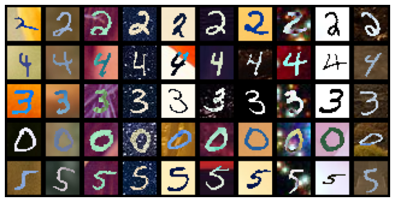
Figure 2: Updated PolyMnist Dataset

We use $\beta$-VAE for training baseline multimodal VAEs and unimodal VAEs with Adam optimizer (Kingma and Ba, 2015). We use an initial learning rate of 0.001, and the models are trained for 200 epochs with $\beta=0.5$ with a latent dimension of 64. Other hyperparameters are discussed in Appendix A.2.

The score networks are trained with an initial learning rate of $0.0002$ using the Adam optimizer. We run annealed Langevin dynamics using different noise levels for $T$ number of steps to generate samples from the score models, and $T$ is tuned using the validation set. See Appendix A.3 for the details of training and sampling using the score model.

For the score model, $\mathbf{z}_{\mathbf{u}}$, missing modalities, are initialized from a Gaussian distribution of $\mathcal{N}(\mathbb{0},\mathbb{1})$.

Conditional generation is done for MVAE and MVTCAE using PoE of the posteriors of given modalities, and for the mixture models, a mixture component is chosen uniformly from the observed modalities.

We evaluate all methods on both prediction coherence and generative quality. To measure the coherence, we use a pre-trained classifier to extract the label of the generated output and compare it with the associated label of the observed modalities. The coherence of the unconditional generation is evaluated by counting the number of consistent predicted labels from the pre-defined classifier. We also measure the generative quality of the generated modalities using the FID score (Heusel et al., 2017).

Figure 3 shows the generated samples from the third modality given the rest. The SBM-VAE generates high-quality images with considerable variation, very close to the training dataset, while the baselines generate more blurry images with a lower variation. We also study, how the conditional coherence and FID change with the number of the observed modality. For an accurate conditional model, we expect as we observed more modalities, the accuracy and quality of conditional generation improve. Figure 5 shows the FID score of the last modality as we increase the given modalities and Figure 5 demonstrates the conditional coherence by measuring the accuracy of the predicted images on the last modality given a different number of observed modalities.

As mentioned by  Daunhawer et al. (2022), the other multimodal VAEs perform poorer and poorer as we give them more modalities as shown by the high FID score of the generated modality while the SBM makes use of the additional modalities to generate better images as we increase the modalities. Even though the other multimodal VAEs have high coherence as expected, they downplay that advantage by decreasing the quality of the image they generate.

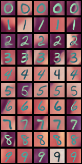
(a) SBM-VAE

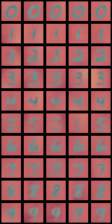
(b) MMVAE+

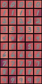
(c) MVTCAE

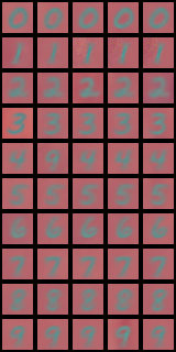
(d) MoPoE

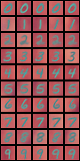
(e) MVAE

Figure 3: Multiple conditionally generated samples for each digit from the third modality. Each column shows samples generated conditionally for each digit given the remaining modalities. (Please see the appendix for the complete set that includes SBM-RAE and MMVAE.)

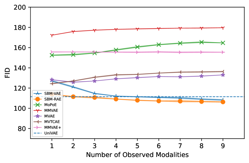
Figure 4: The conditional FID of the last modality generated by incrementing the given modality at a time. The x-axis shows how many modalities are given to generate the modality and the y-axis shows the FID score of the generated modality.

Figure 5: The conditional accuracy of the last modality generated by incrementing the given modality at a time. The x-axis shows how many modalities are given to generate the modality and the y-axis shows the accuracy of the generated modality.

As also noted by  Daunhawer et al. (2022), the generation quality of the baseline multimodal VAEs degrades by observing more modalities while the generation quality of our methods consistently improves as we observe more modalities. This behavior is consistent with what we expect from a valid conditional distribution. We also show the generation quality of uni-modal VAE for the same modality. SBM-VAE and SBM-RAE show slightly better generation quality than the uni-modal VAE, which is due to our claim that conditional prior described by $p_{\theta}(\mathbf{z}_{k}|\mathbf{z}_{-k})$ is closer $q(\mathbf{z}_{k}|\mathbf{x}_{k})$ than the standard Gaussian prior $p(\mathbf{z})$.

Similarly, the predicted accuracy of our method improves as we observed more modalities, however, when in the presence of one or two observed modalities, the accuracy of SBM-VAE and SBM-RAE is considerably lower than the baseline methods. This behavior is attributable to the sampling complexity from $p_{\theta}(\mathbf{z}_{-k}|\mathbf{z}_{k})$ as Langevin dynamics has to explore much larger space, but as we observe more modality the conditional distribution becomes simpler and we can generate better samples.

We also study unconditional coherence, which has been reported in Figure  6, shows the unconditional coherence of the generated modalities. We evaluate unconditional accuracy by counting the number of consistent labels across different modalities after classifying the generated images using a pre-trained classifier. $84.5\%$ of generated images using SBM-RAE are coherent over nine modalities, which is considerably higher than the next-best MMVAE. Our result shows that MVTCAE performs poorly in unconditional generation.

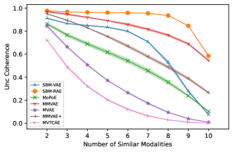
Figure 6: Unconditional coherence. The x-axis shows the number of modalities the coherence is calculated and the y-axis shows the coherence.

Finally, we study the scalability of methods given a different number of data modalities (see Figure 7). We first train the models with different numbers modalities and then evaluate unconditional FID, Conditional FID for the first modality given the rest, and conditional accuracy of the first modality. The performance of our proposed methods is consistent across a different number of data modalities. Specifically, both SBM-VAE and SBM-RAE show consistent conditional FID, for which the complexity of the sampling from prior remains the same as we increase the number of data modalities.

Further ablation studies regarding model architecture and the effect of $beta$ values as well as more generated samples have been reported in Appendix A.4

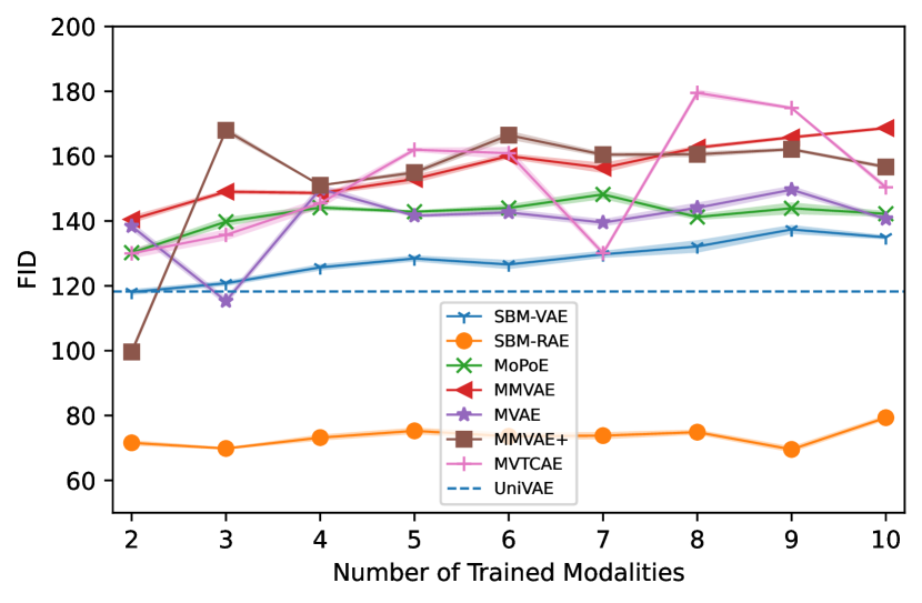
(a) Unconditional fid

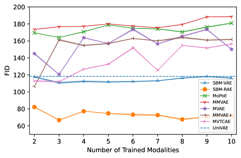
(b) Conditional fid

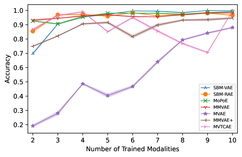
(c) Conditional accuracy

Figure 7: Result of unconditional generation (a) and the first modality generated by incrementing the modalities the model is trained on (b and c). The x-axis shows how many modalities the model was trained on and the y-axis shows the result of the generated modality.

4.2 CelebAMask-HQ

Figure 8: A sample of image and associated mask from the CelebAMask-HQ dataset (Attribute not shown)

The images, masks, and attributes of the CelebAMask-HQ dataset can be treated as different modalities of expressing the visual characteristics of a person. A sample from the dataset is shown in figure 8. The images and masks are resized to 128 by 128. The masks are either white or black where all the masks given in the CelebAMask-HQ except the skin mask are drawn on top of each other as one image. We follow the pre-processing of selecting 18 out of 40 existing attributes as described in Wu and Goodman (2018). We compare SBM-VAE, SBM-RAE, MoPoE, MVTCAE, and MMVAE+. See Appendix A.5 for the experimental setups of these methods.

We evaluate the generation quality of the image modality using FID score and generation accuracy of mask and attribute modalities using sample-average $F_{1}$ score. Table 1 shows how our methods compare with the baselines in the presence of no observed modalities, one or two modalities. We have also reported the performance of a supervised model trained to predict attributes directly given to images. SBM-VAE generates high-image quality, compared to baselines, in both conditional and unconditional settings, while on the mask and attribute modalities, MoPoE shows better performance.

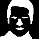
Male +

Mouth_Slightly_Open +

Straight_Hair

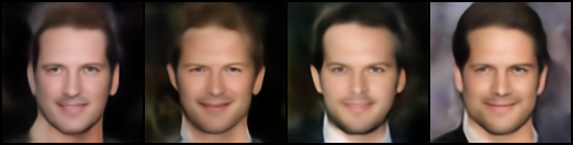
Male +

Gray_Hair +

Straight_Hair

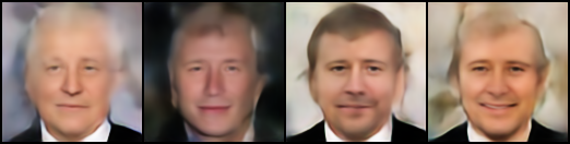
(a) SBM-VAE output

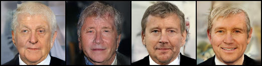
(b) DiffuseVAE output

Figure 10: Higher quality image generation using DiffuseVAE given mask and attribute shown in the first two columns

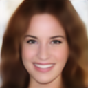
Mouth_Slightly +

_Open Smiling +

Brown_Hair +

Wavy_Hair +

Heavy_Makeup

(a) SBM-RAE

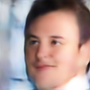
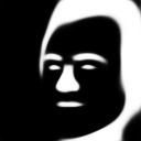
Male

(b) SBM-VAE

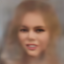
Mouth_Slightly +

_Open Smiling +

Blond_Hair +

Heavy_Makeup

(c) MoPoE

Figure 13: Unconditional Generation

Table 1: CelebAMask-HQ Result

	Attribute		Mask		Image
GIVEN	Both	Img	Both	Img	Both	Mask	Attr	Unc
	F1	F1	F1	F1	FID	FID	FID	FID
SBM-RAE	0.67	0.66	0.84	0.84	96	98	94	92
SBM-VAE	0.65	0.60	0.85	0.84	84	82	87	84
MoPoE	0.68	0.71	0.85	0.91	144	132	194	158
MVTCAE	0.7	0.68	0.87	0.87	105	92	95	200
MMVAE+	0.64	0.69	0.81	0.91	132	129	166	246
Supervised		0.79
SBM-VAE with DiffuseVAE					25	23	32	27

Since variational autoencoders suffer from low-quality and blurry images, compared to other SOTA generative models such as diffusion models (Dhariwal and Nichol, 2021), in order to get higher-quality images, we use DiffuseVAE model (Pandey et al., 2022) on the output of the generated images. We illustrate the generated samples from SBM-VAE and augmented DiffuseVAE in Figure10 to state the final outcome will respect the conditioned modalities. As the figure shows, the quality of the images is much better while preserving the attributes and the masks given to generate them.

Finally, we show the unconditional generation across different modalities using SBM-RAE, SBM-VAE, and MoPoE in Figure 13. Please see Appendix A.6 for more qualitative samples and ablation studies on the CelebAMask-HQ dataset.

5 Conclusion and Discussion

Multimodal VAEs are an important tool for modeling multimodal data. In this paper, we provide a different multimodal posterior using score-based models. Our proposed method learns the correlation of latent spaces of unimodal representations using a joint score model in contrast to the traditional multimodal VAE ELBO. We show that our method can generate better-quality samples and at the same time preserves coherence between modalities. We have also shown that our approach is scalable to multiple modalities. SBM-VAE provided better quality but lower coherence compared to SBM-RAE. This work can be further expanded upon in future research with more complex autoencoder models for even higher performance.

Appendix A Appendix

A.1 SBM-RAE

Regularized autoencoders (RAEs) [Ghosh et al., 2020] can be used instead of VAEs in our setting. RAEs assume a deterministic encoder and regularize the latent space directly by penalizing $L_{2}$ norm of the latent variables:

$$\mathcal{L}_{\text{RAE}}=\mathcal{L}_{\text{REC}}+\beta||\mathbb{z}||_{2}^{2}+\lambda\mathcal{L}_{\text{REG}},$$ (8)

where $L_{\text{REC}}$ is the reconstruction loss for deterministic autoencoder and $L_{\text{REG}}$ is the decoder regularizer. In our setup, we don’t use any decoder regularizer.

In order to generate a sample from the latent space, RAEs require to fit separate density estimators on the latent variables. In our case, the score models are responsible for generating samples from the latent space, which makes RAE a compelling choice for our setup. RAEs are capable of learning more complex latent structures, and expressive generative models such as score models can effectively learn that structure to generate high-quality samples.

A.2 Model Architectures and Experimental setups for Extended PolyMNIST

The extended PolyMnist dataset was updated from the original PolyMnist dataset by Sutter et al. [2020] with different background images and ten modalities. It has 50,000 training set, 10,000 validation set, and 10,000 test set. The VAEs for each modality are trained with an initial learning rate of $0.001$ using a $\beta$ value of $0.5$ where all the prior, posterior, and likelihood are Gaussians. This also applies to all multimodal VAEs except MMVAE+ which uses Laplace distribution instead of Gaussian. The RAE for each modality was trained using the mean squared error loss with the norm of $||\mathbb{z}||_{2}^{2}$ regularized by a factor of $10^{-5}$ and a Gaussian noise added to $z$ before feeding to the decoder with mean $0$ and variance of $0.01$ where the hyperparameter values were tuned using the validation set. The encoders and decoders for all models use residual connections to improve performance and are similar in structure to the architecture used in Daniel and Tamar [2021] with a latent size of 64. For MMVAE+, modality-specific and shared latent sizes are each 32 and the model was trained similarly to the code provided by the paper with the DREG estimator where K=1. The detailed architecture can be found by referring to the code that will be released.

The neural net of SBM-VAE for this dataset is made up of a simple multi-layer perceptron (MLP) with softplus activation where the $\mathbb{z}$s from the VAEs of all the modalities are concatenated and fed into the model while SBM-RAE required a more complex network and a UNET like model was used with the latent space reshaped into a size of 8x8. For an exact comparison of the two SBMs using the same model is shown in the section A.4. We assume all modalities are present during training. To train the SBMs, we generate the samples from the encoders of each modality and minimize the denoising score matching objective shown in eq. 3. For SBM-VAE, samples are taken from the posterior at training time and the mean of posterior is taken at inference time. For SBM-RAE, the $\mathbb{z}$s are taken directly. We use a learning rate of $0.0002$ with the Adam optimizer [Kingma and Ba, 2015]. The detailed hyperparameters are shown in table 2.

Table 2: Score Hyperparameters PolyMnist

Model	Generation type	$\sigma_{min}$	$\sigma_{max}$	len($\sigma$s)	LD iters	$\lambda_{1}$	$\lambda_{2}$
SBM-VAE	conditional	1	1	1	40	0.2	0.032
	unconditional	1	1	1	40	0.1	0.335
SBM-RAE	conditional	0.1	5	200	20	0.002	0.5
	unconditional	0.1	5	200	2	0.01	0.7

A.3 Training and Inference Algorithm

We follow the Song and Ermon [2019, 2020] to train the score models using the latent representation from the encoders. The following algorithms 1, 2 show the training and inference algorithm we use.

Algorithm 1 Training

$M$, $N$, $\sigma$s $\triangleright$ M - modality, N -epochs, $\sigma$s - noise levels

$\mathbb{Z}$ = []

for $i=1$ to $M$ do

     Get $\mathbb{x}_{i}$ $\triangleright$ Get the input x from modality i

     Sample $\mathbb{z}_{i}$ from $q(\mathbb{z|x}_{i})$ $\triangleright$ Sample z from the encoder

     Append $\mathbb{z}_{i}$ to $\mathbb{Z}$

end for

for $epoch=1$ to $N$ do

     t = random_sample_index(1,len($\sigma$s)) $\triangleright$ sigma index t

     Compute $\mathbb{s}_{\theta}(\mathbb{Z},t)/\sigma_{t}$

     Calculate loss using equation 3 multiplied by $\sigma_{t}^{2}$

     Backpropagate and update the weights of the SBM

end for

Algorithm 2 Inference

$\sigma$s, $n$, $\lambda_{1}$, $\lambda_{2}$ $\triangleright$ n is number of LD iterations

if Unconditional then

     Sample $\mathbb{z}$ from $\mathcal{N}(\mathbb{0},\mathbb{I})$ and stack to get $\mathbb{Z}$

else if Conditional then

     Sample $\mathbb{z}$ from $\mathcal{N}(\mathbb{0},\mathbb{I})$ if missing

     Sample $\mathbb{z}$ from encoder $q(\mathbb{z|x}_{i})$ if present

     Stack all $\mathbb{z}$ to get $\mathbb{Z}$

end if

for t, $\sigma$ in $\sigma$s do $\triangleright$ t - sigma index

     $\alpha=\lambda_{1}*\sigma_{t}^{2}/\sigma_{T}^{2}$

     for $i=1$ to $n$ do

         Update missing $\mathbb{z}$s by the following equation 13

         $\mathbb{z}^{t+1}=\mathbf{z}^{t}+\alpha*\mathbb{s}([\mathbb{z}^{t},\mathbf{z_{o}}],t)/\sigma_{t}+\lambda_{2}\sqrt{2\alpha}\mathcal{N}(\mathbb{0},\mathbb{I})$ $\triangleright$ $\lambda_{1}$, $\lambda_{2}$ are LD hyperparameters

     end for

end for

Feed the $\mathbb{z}$ to the respective decoder to get output

A.4 Ablation study

A.4.1 Fine-tunning the generative models using missing modalites

We can further finetune the generative model (decoder) to increase the overall coherence. During training, we assume all the modalities are present. This condition is necessary for training $p_{\theta}$ in the described setup . However, we are interested in conditional queries of $p(.|\mathbf{x}_{\mathbf{o}})$, we can achieve a tighter lower bound by further optimizing the $p_{\psi}(\mathbf{x}_{\mathbf{u}}|\mathbf{z}_{u})$ for sample from $q(\mathbf{z}_{\mathbf{u}}|\mathbf{z}_{\mathbf{o}},\mathbf{x}_{\mathbf{o}})$. We update the parameters of decoders to maximize the conditional log-likelihood:

$$\max_{\psi}\mathbb{E}_{q(\mathbf{z}_{\mathbf{u}}|\mathbf{z}_{\mathbf{o}},\mathbf{x}_{\mathbf{o}})}\log p_{\psi}(\mathbf{x}_{\mathbf{u}}|\mathbf{z}_{\mathbf{u}})$$

$$=\max_{\psi}\frac{1}{K}\sum_{k=1}^{K}\log p_{\psi_{k}}(\mathbf{x}^{k}_{\mathbf{u}}|\mathbf{z}^{k}_{\mathbf{u}})\quad z^{k}_{\mathbf{u}}\sim q(.|\mathbf{z}_{\mathbf{o}},\mathbf{x}_{\mathbf{o}})$$ (9)

For each training example in the batch, we randomly drop each modality with probability $p$. Eq. 9 will increase the likelihood of the true assignment of the dropped modalities given the observed modalities.

Figure  15 shows the conditional coherence of different finetuned models with varying $p$. As it can be seen in the figure, the coherence improves by a small amount but the downside of this is that it comes with worse FID values due to the fact we are only finetuning the generative model of the VAE.

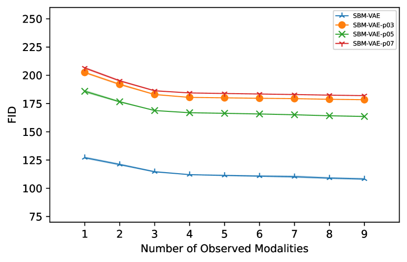
Figure 14: Plot of finetuning experiment using different $p$ values on how it affects conditional FID. The conditional FID of the last modality generated by incrementing the given modality at a time. The x-axis shows how many modalities are given to generate the modality and the y-axis shows the FID of the generated modality.

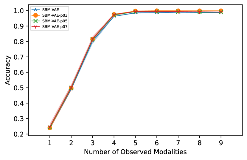
Figure 15: Plot of finetuning experiment using different $p$ values on how it affects conditional coherence. The conditional accuracy of the last modality generated by incrementing the given modality at a time. The x-axis shows how many modalities are given to generate the modality and the y-axis shows the accuracy of the generated modality.

Table 3 shows the conditional performance when any modality is dropped by a probability $p$ from 0.1 to 0.9. The table also includes finetuned SBMVAE (SBMVAE-ft) evaluations in addition to all models. SBMVAE-ft with drop probability 0.5 improves the overall coherence of SBMVAE by some amount. Figure 17 and 17 show the conditional coherence and FID of the last 5 modalities given the first 5 modalities.

Table 3: Conditional Coherence with different amounts of data given

Model	Drop Probability
	$0.1$	$0.3$	$0.5$	$0.7$	$0.9$	Avg
MoPoE	0.981	0.969	0.943	0.885	0.838	0.923
MMVAE	0.979	0.979	0.980	0.979	0.980	0.979
MVAE	0.891	0.848	0.800	0.717	0.575	0.766
MVTCAE	0.988	0.975	0.953	0.850	0.678	0.888
MMVAE+	0.945	0.939	0.941	0.941	0.942	0.942
SBMRAE	0.949	0.944	0.896	0.686	0.425	0.78
SBMVAE	0.984	0.932	0.875	0.671	0.277	0.747
SBMVAE-ft-0.1	0.997	0.980	0.873	0.600	0.270	0.744
SBMVAE-ft-0.3	0.993	0.975	0.842	0.539	0.336	0.737
SBMVAE-ft-0.5	0.996	0.994	0.915	0.700	0.260	0.773
SBMVAE-ft-0.7	0.969	0.944	0.893	0.588	0.279	0.734
SBMVAE-ft-0.9	0.799	0.802	0.753	0.534	0.236	0.624

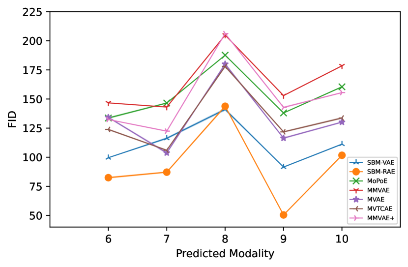
Figure 16: Conditional FID of the last 5 modalities given the first 5 modalities.

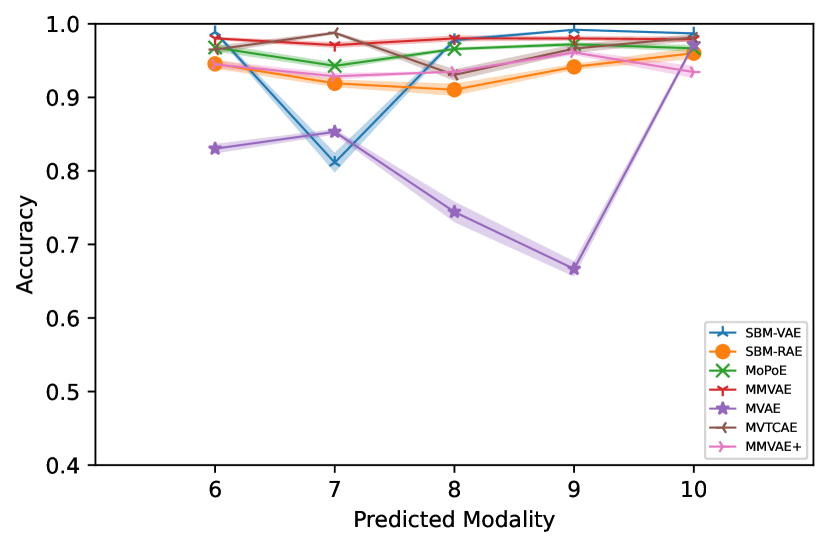
Figure 17: Conditional coherence of the last 5 modalities given the first 5 modalities.

A.4.2 SBM model ablation

In the experiment section of the paper, we used an MLP for the score model of SBM-VAE and a UNET model for SBM-RAE. Here we show the results of SBM-VAE using an MLP and a UNET model same as SBM-RAE. A similar result 19 structure is exhibited by SBM-VAE using this model but the coherence is a little lower. This shows that SBM-VAE can work well in simpler models. While this is true SBM-VAE, SBM-RAE couldn’t generate good results using this simple model and therefore not shown here. The sample from the conditionally generated second modality is also shown as a reference in figure 20.

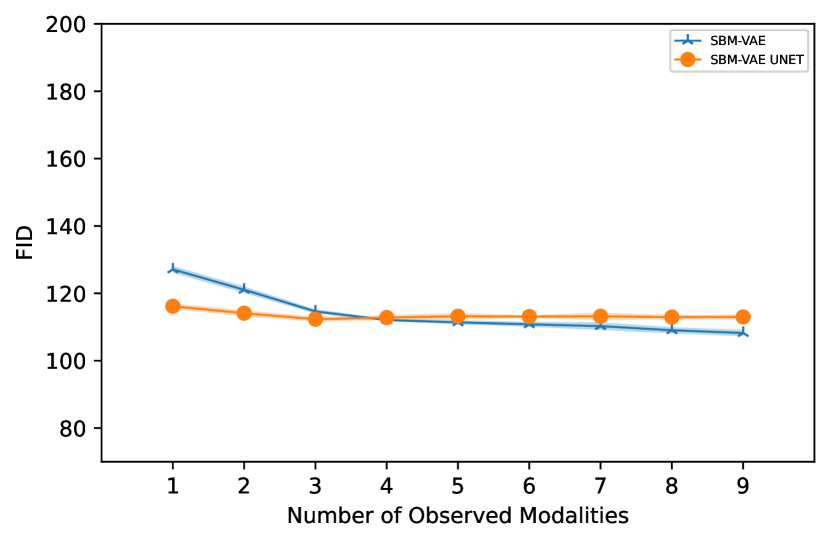
Figure 18: The conditional fid of the last modality generated by incrementing the given modality at a time. The x-axis shows how many modalities are given to generate the modality and the y-axis shows the FID score of the generated modality.

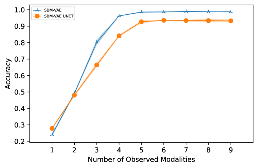
Figure 19: The conditional accuracy of the last modality generated by incrementing the given modality at a time. The x-axis shows how many modalities are given to generate the modality and the y-axis shows the accuracy of the generated modality.

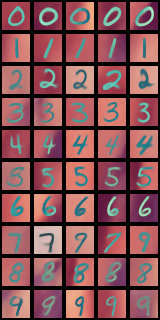
Figure 20: SBM-VAE (UNET)

A.4.3 Different hyperparameter values

Here we repeat experiments of Fig 4 and 5 with $\beta$ values of 0.1, 1, and 5 in addition to 0.5. MVTCAE wasn’t stable on $\beta=0.1$ and the result of that is skipped. Also, on $\beta=5$, we show MMVAE, MoPoE, MMVAE+, and MVTCAE. Figure 28 and 28 also show increase latent size for some baselines which don’t have modality-specific latents and compare it with MMVAE+, SBM-VAE, and SBM-RAE unchanged.

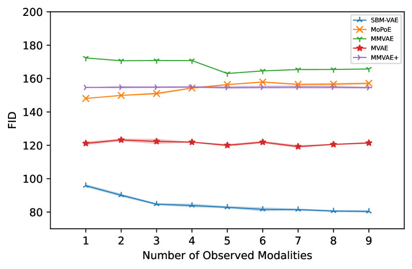
Figure 21: Similar to Fig 4 with $\beta$=0.1.

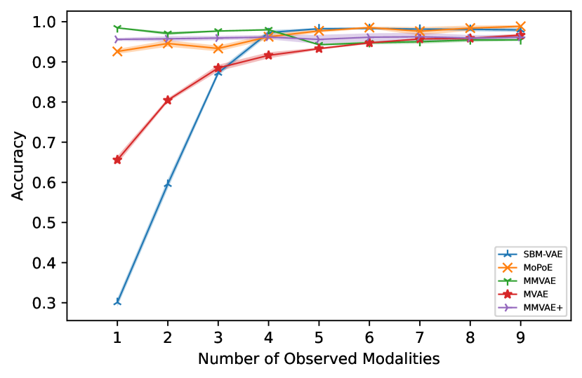
Figure 22: Similar to Fig 5 with $\beta$=0.1.

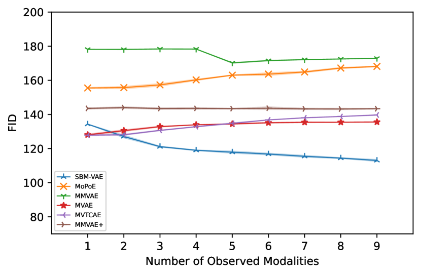
Figure 23: Similar to Fig 4 with $\beta$=1.

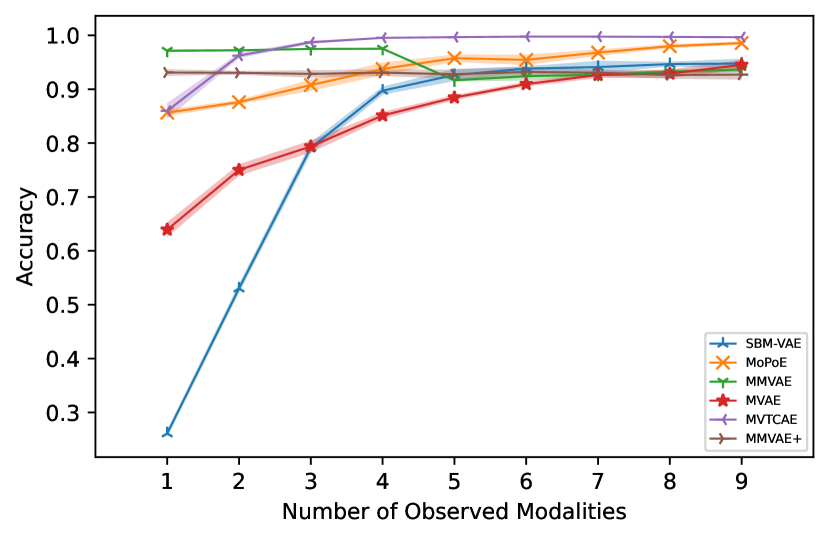
Figure 24: Similar to Fig 5 with $\beta$=1.

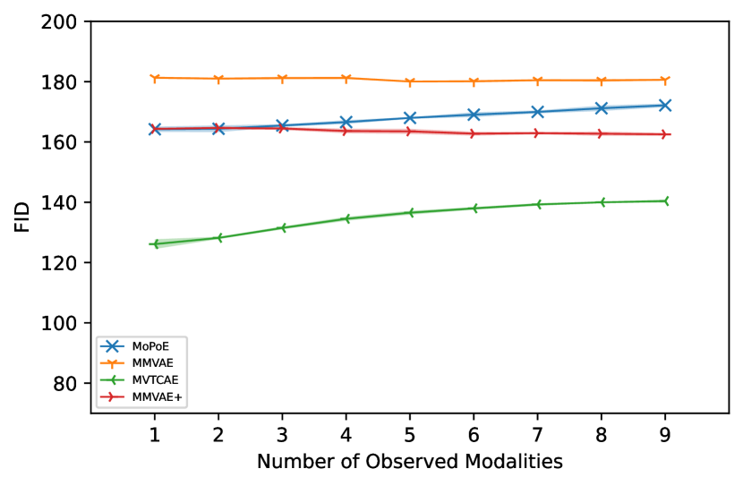
Figure 25: Similar to Fig 4 with $\beta$=5.

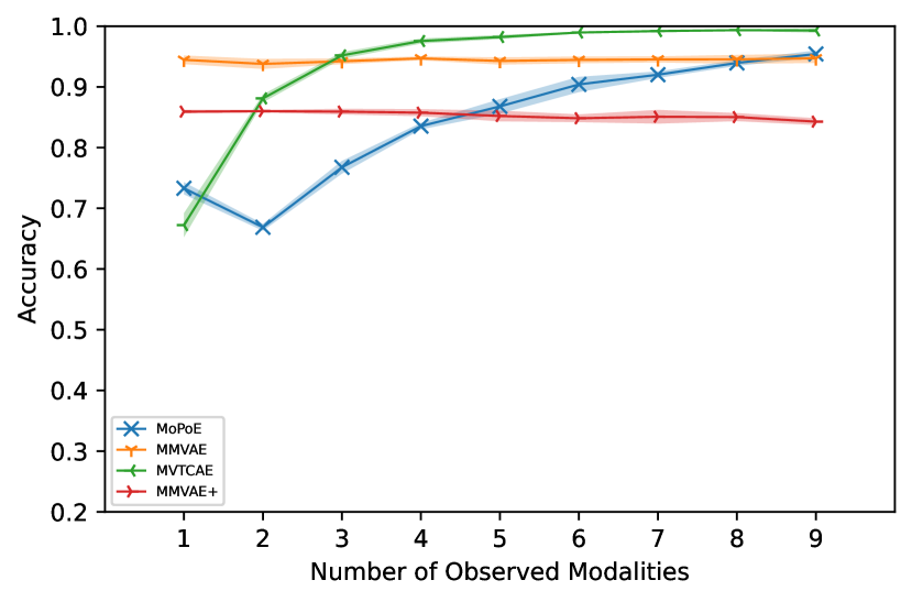
Figure 26: Similar to Fig 5 with $\beta$=5.

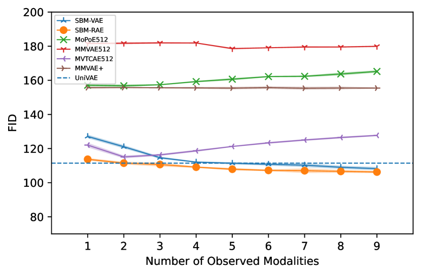
Figure 27: Similar to Fig 4 with the size of z=512 for some baselines.

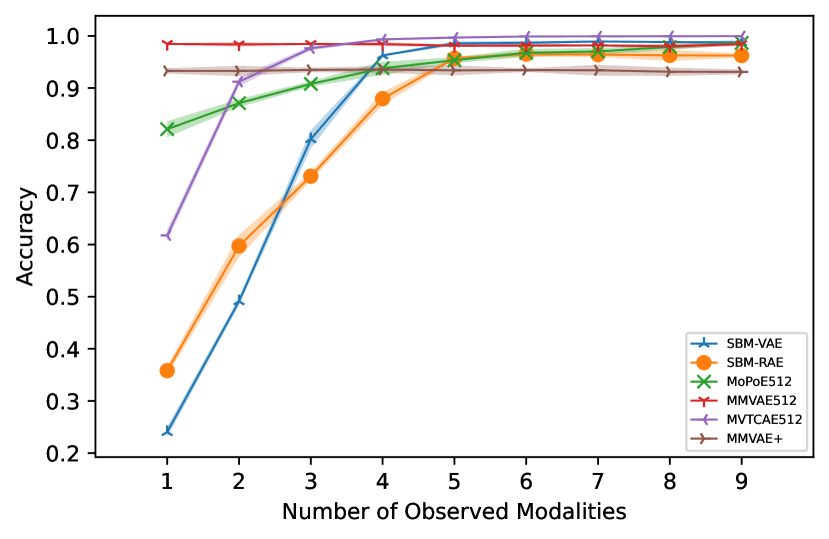
Figure 28: Similar to Fig 5 with the size of z=512 for some baselines.

A.4.4 Qualitative Results for Extended PolyMNIST

Here we show some conditionally generated samples and unconditional generation from each model. Conditional samples are shown in figures 30 and 31 and unconditional samples in figure 32.

(a) SBM-VAE

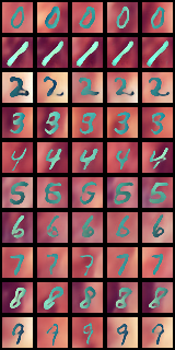
(b) SBM-RAE

(c) MMVAE+

(d) MVTCAE

(e) MoPoE

(f) MMVAE

(g) MVAE

Figure 29: Conditional Samples from the third modality given the rest

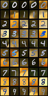
(a) SBM-VAE

(b) SBM-RAE

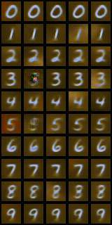
(c) MMVAE+

(d) MVTCAE

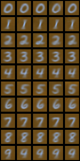
(e) MoPoE

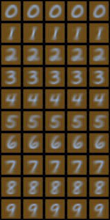
(f) MMVAE

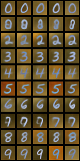
(g) MVAE

Figure 30: Conditional Samples from the first modality given the rest

(a) SBM-VAE

(b) SBM-RAE

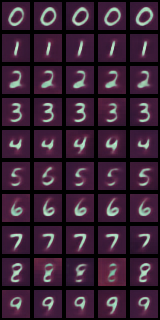
(c) MMVAE+

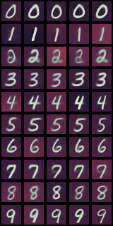
(d) MVTCAE

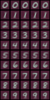
(e) MoPoE

(f) MMVAE

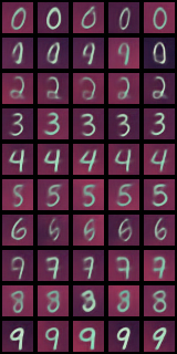
(g) MVAE

Figure 31: Conditional Samples from the sixth modality given the rest

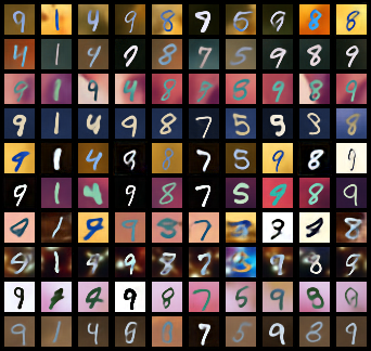
(a) SBM-VAE

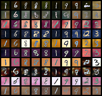
(b) SBM-RAE

(c) MMVAE+

(d) MVTCAE

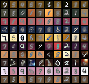
(e) MoPoE

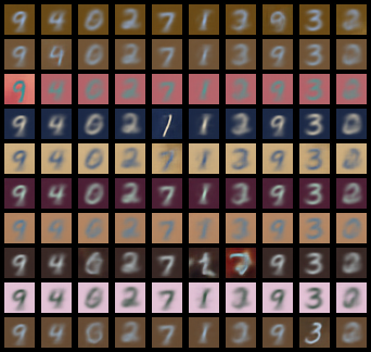
(f) MMVAE

(g) MVAE

Figure 32: Unconditional Samples where each of the columns are unconditional samples from each modality

A.5 CelebMaskHQ Experimental Setup

The CelebMaskHQ dataset is taken from Lee et al. [2020] where the images, masks, and attributes are the three modalities. All face part masks were combined into a single black-and-white image except the skin mask. Out of the 40 attributes, 18 were taken from it similar to the setup of Wu and Goodman [2018]. The encoder and decoder architectures are similar to Daniel and Tamar [2021] and a latent size of 256 was used for all models. For MMVAE+, modality-specific and shared latent sizes are each 128 trained with DREG estimator with K=1. For SBM-VAE, the image VAE was trained using Gaussian likelihood, posterior, and prior with $\beta=0.1$. The same applies for the mask VAE but with $\beta=1$. The attribute VAE uses Gaussian prior and posterior with a bernoulli likelihood. This applies to all other baselines with the exception of MMVAE+ which uses laplace likelihood and prior. All baselines use $\beta=1$ that was selected from three $\beta$ values of 0.1, 0.5, and 1 using validation data. For SBM-RAE, $\beta$ values of $10^{-4}$, $10^{-5}$, $10^{-4}$ and Gaussian noises of mean $0$ and variance of $0.001$, $0.001$, $0.1$ were added to $z$ before feeding to the decoder for the image, mask, and attribute modality respectively.

The score-based models use a UNET architecture with the latent size reshaped into a size of 16x16. We take the mean of the posterior during training and inference time for SBM-VAE where as the $\mathbb{z}$ were taken during both times for SBM-RAE. Table 4 shows the detailed hyperparameters used for the score models. DiffuseVAE hyperparameters and models are the same ones used in Pandey et al. [2022] with formulation 1 for the 128x128 CelebHQ dataset.

Table 4: Score Hyperparameters CelebMaskHQ
Multiple values are values for (image,mask,attr)

Model	Type	$\sigma_{min}$	$\sigma_{max}$	len($\sigma$s)	LD iter	$\lambda_{1}$	$\lambda_{2}$
SBM-VAE	given 1	0.1	5	500	2	0.016,0.015,0.015	0.8,0.5,0.5
	given 2	0.1	5	500	2	0.018,0.015,0.015	0.8,0.5,0
	unc	0.1	5	500	2	0.01	0.8
SBM-RAE	given 1	0.1	5	500	2	0.016,0.015,0.015	0.8,0.5,0.5
	given 2	0.1	5	500	2	0.02,0.015,0.015	0.8,0.5,0.5
	unc	0.1	5	500	2	0.01	0.8

A.6 CelebA Ablation

Here we show results from a model trained on the image and attribute modality from the CelebHQ dataset. As a comparison, we also add one of the baselines (MoPoE). Table  5 shows the results.

Table 5: CelebHQ on two modalities result

	Attribute	Image
GIVEN	Img	Attr	None (Unc)
	F1	FID	FID
SBM-RAE	0.65	97	112
SBM-VAE	0.60	94	92
MoPoE	0.66	203	133

A.6.1 CelebMaskHQ

In this section, we show samples from the CelebHQMASK dataset where the generated images are conditioned on different modalities. Figure 34 shows unconditionally generated outputs from each modality. Figure 35 shows different samples where only the image is given, Figure 36 shows different samples where the mask is given, Figure 37 shows different samples where the attribute is given. Figures 39, 38, 40 show different samples where a combination of the two modalities are given and the remaining modality is predicted.

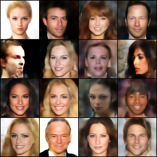
(a) SBM-RAE image

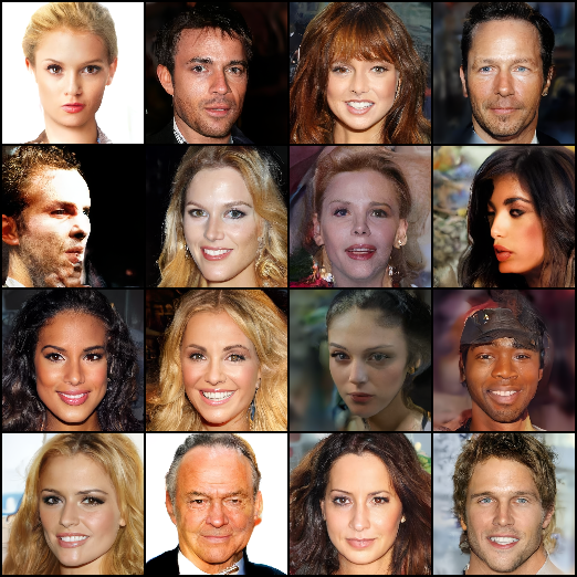
(b) DifuseVAE output

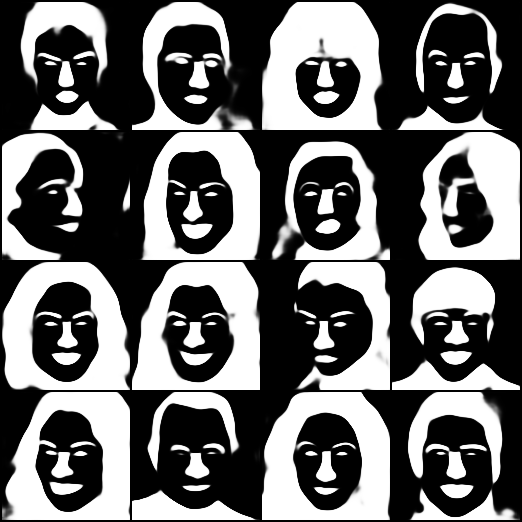
(c) SBM-RAE mask

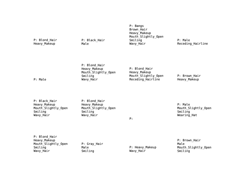
(d) SBM-RAE attribute

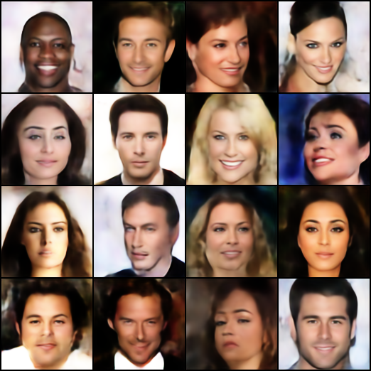
(e) SBM-VAE image

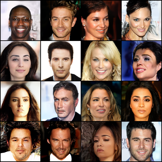
(f) DifuseVAE output

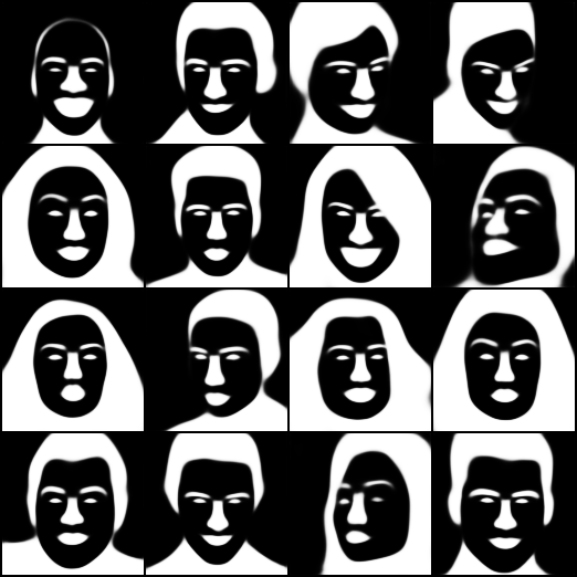
(g) SBM-VAE mask

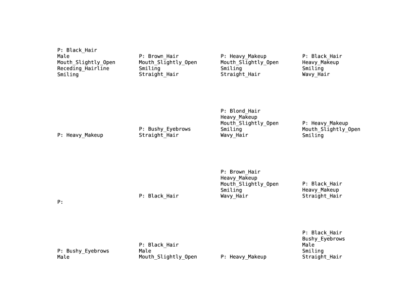
(h) SBM-VAE attribute

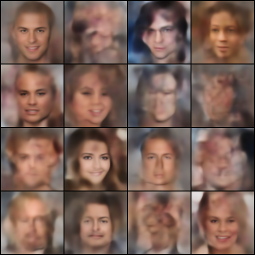
(i) MoPoE image

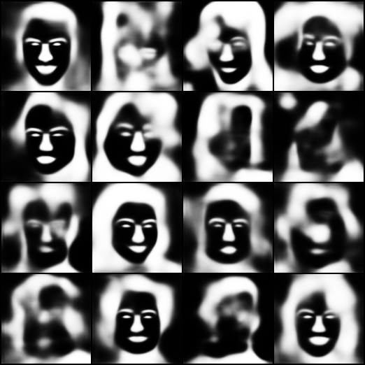
(j) MoPoE mask

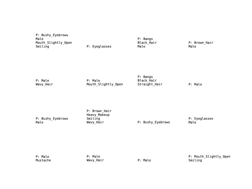
(k) MoPoE attribute

Figure 34: Unconditional generation

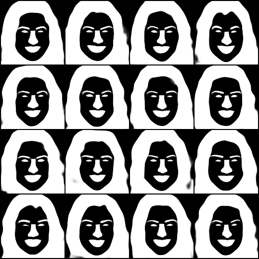
(a) SBM-RAE mask

(b) SBM-RAE attribute

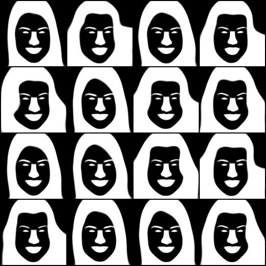
(c) SBM-VAE mask

(d) SBM-VAE attribute

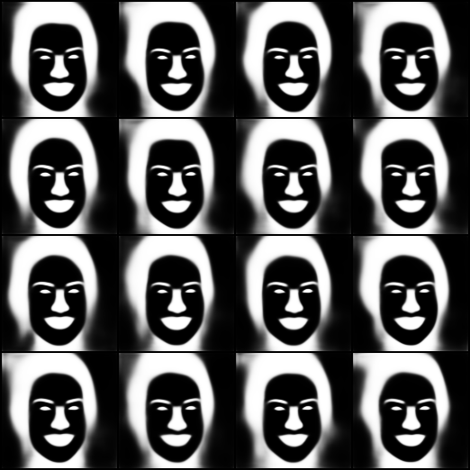
(e) MoPoE mask

(f) MoPoE attribute

Figure 35: Mask and Attribute generation given Image

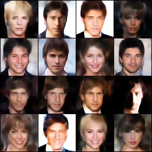
(a) SBM-RAE image

(b) SBM-RAE attribute

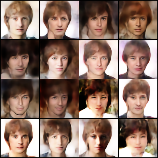
(c) SBM-VAE image

(d) SBM-VAE attribute

(e) MoPoE image

(f) MoPoE attribute

Figure 36: Image and Attribute generation given Mask

Black_Hair +

Bushy_Eyebrows +

Male +

Mustache +

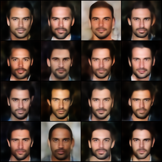
(a) SBM-RAE image

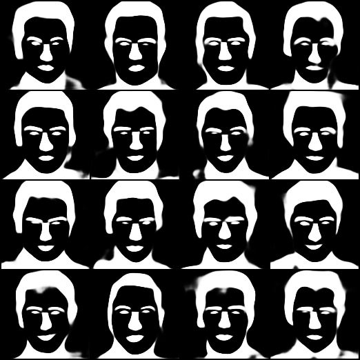
(b) SBM-RAE mask

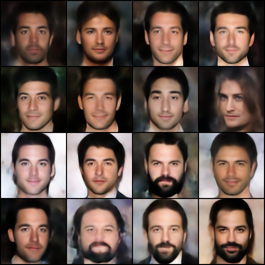
(c) SBM-VAE image

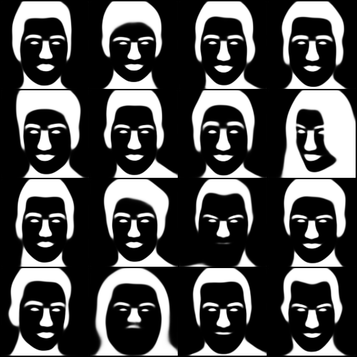
(d) SBM-VAE mask

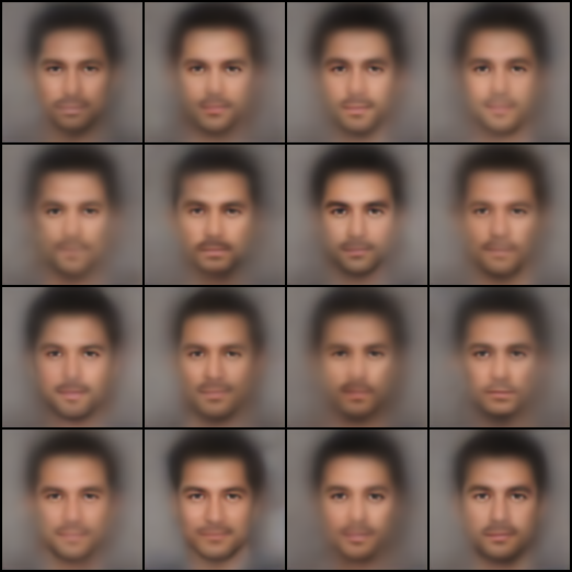
(e) MoPoE image

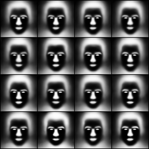
(f) MoPoE mask

Figure 37: Image and Mask generation given Attribute

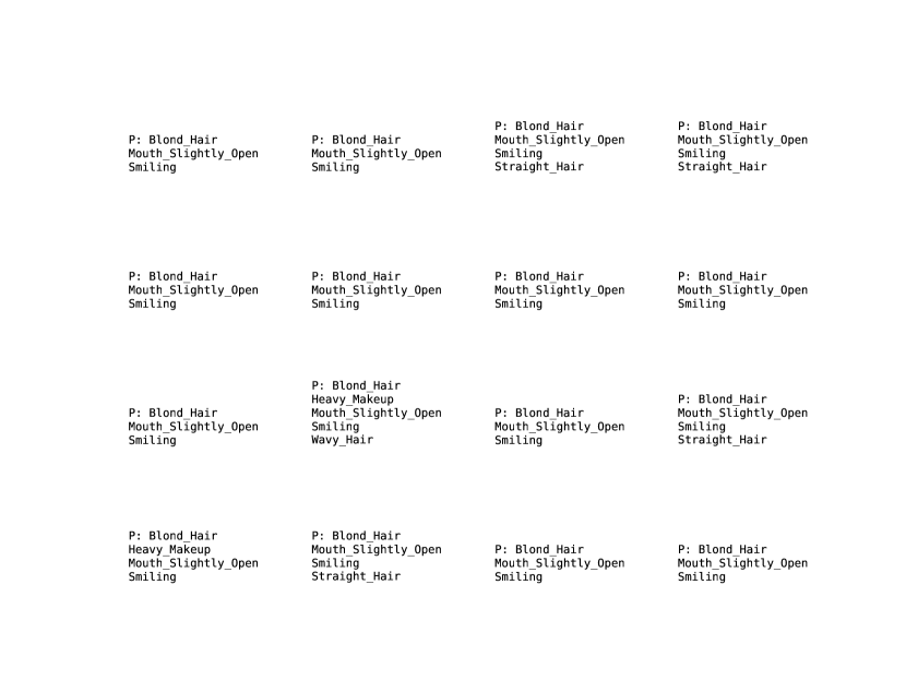
(a) SBM-RAE

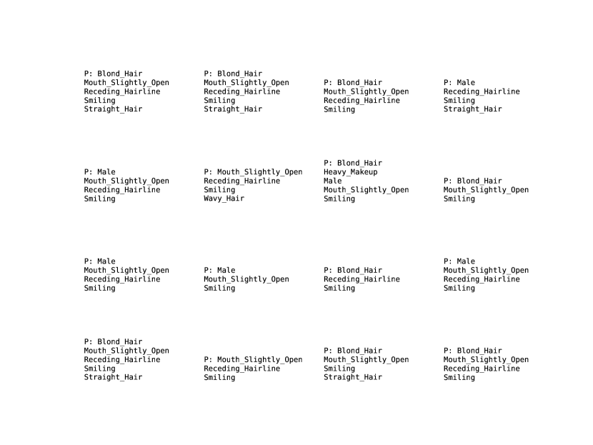
(b) SBM-VAE

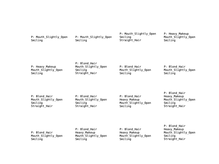
(c) MoPoE

Figure 38: Attribute generation given Image and Mask

Mouth_Slightly_Open +

Smiling +

Wavy_Hair +

(a) SBM-RAE

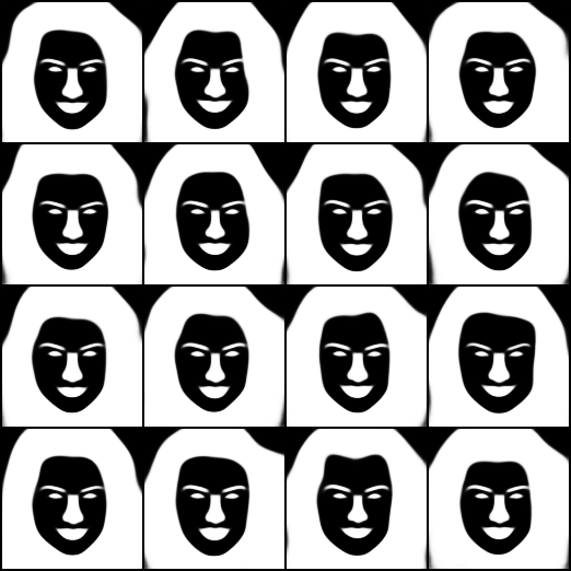
(b) SBM-VAE

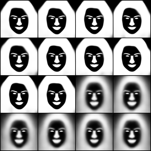
(c) MoPoE

Figure 39: Mask generation given Image and Attribute

Mouth_Slightly_Open +

Receding_Hairline +

Smiling +

Wavy_Hair +

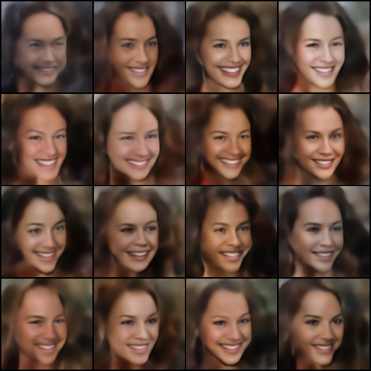
(a) SBM-RAE

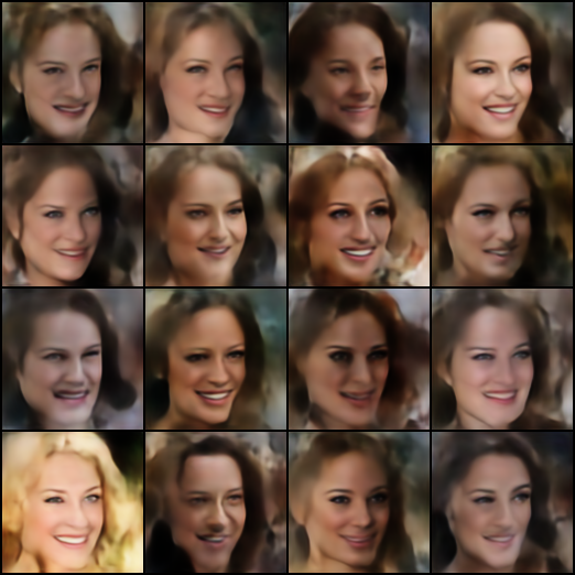
(b) SBM-VAE

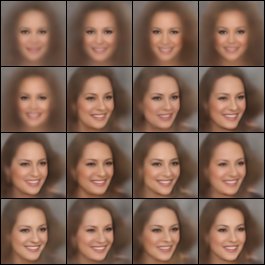
(c) MoPoE

Figure 40: Image generation given Mask and Attribute

References

- Daniel and Tamar [2021] Tal Daniel and Aviv Tamar. Soft-introvae: Analyzing and improving the introspective variational autoencoder. In Proceedings of the IEEE/CVF Conference on Computer Vision and Pattern Recognition (CVPR), pages 4391–4400, June 2021.
- Daunhawer et al. [2022] Imant Daunhawer, Thomas M. Sutter, Kieran Chin-Cheong, Emanuele Palumbo, and Julia E Vogt. On the limitations of multimodal VAEs. In International Conference on Learning Representations, 2022. URL https://openreview.net/forum?id=w-CPUXXrAj.
- Dhariwal and Nichol [2021] Prafulla Dhariwal and Alexander Quinn Nichol. Diffusion models beat gans on image synthesis. In Marc’Aurelio Ranzato, Alina Beygelzimer, Yann N. Dauphin, Percy Liang, and Jennifer Wortman Vaughan, editors, Advances in Neural Information Processing Systems 34: Annual Conference on Neural Information Processing Systems 2021, NeurIPS 2021, December 6-14, 2021, virtual, pages 8780–8794, 2021. URL https://proceedings.neurips.cc/paper/2021/hash/49ad23d1ec9fa4bd8d77d02681df5cfa-Abstract.html.
- Ghosh et al. [2020] Partha Ghosh, Mehdi S. M. Sajjadi, Antonio Vergari, Michael Black, and Bernhard Scholkopf. From variational to deterministic autoencoders. In International Conference on Learning Representations, 2020. URL https://openreview.net/forum?id=S1g7tpEYDS.
- Heusel et al. [2017] Martin Heusel, Hubert Ramsauer, Thomas Unterthiner, Bernhard Nessler, and Sepp Hochreiter. Gans trained by a two time-scale update rule converge to a local nash equilibrium. In I. Guyon, U. Von Luxburg, S. Bengio, H. Wallach, R. Fergus, S. Vishwanathan, and R. Garnett, editors, Advances in Neural Information Processing Systems, volume 30. Curran Associates, Inc., 2017. URL https://proceedings.neurips.cc/paper_files/paper/2017/file/8a1d694707eb0fefe65871369074926d-Paper.pdf.
- Hwang et al. [2021] HyeongJoo Hwang, Geon-Hyeong Kim, Seunghoon Hong, and Kee-Eung Kim. Multi-view representation learning via total correlation objective. In M. Ranzato, A. Beygelzimer, Y. Dauphin, P.S. Liang, and J. Wortman Vaughan, editors, Advances in Neural Information Processing Systems, volume 34, pages 12194–12207. Curran Associates, Inc., 2021. URL https://proceedings.neurips.cc/paper_files/paper/2021/file/65a99bb7a3115fdede20da98b08a370f-Paper.pdf.
- Hyvärinen and Dayan [2005] Aapo Hyvärinen and Peter Dayan. Estimation of non-normalized statistical models by score matching. Journal of Machine Learning Research, 6(4), 2005.
- Kingma and Ba [2015] Diederik P. Kingma and Jimmy Ba. Adam: A method for stochastic optimization. In Yoshua Bengio and Yann LeCun, editors, 3rd International Conference on Learning Representations, ICLR 2015, San Diego, CA, USA, May 7-9, 2015, Conference Track Proceedings, 2015. URL http://arxiv.org/abs/1412.6980.
- Kingma and Welling [2014] Diederik P. Kingma and Max Welling. Auto-encoding variational bayes. In Yoshua Bengio and Yann LeCun, editors, 2nd International Conference on Learning Representations, ICLR 2014, Banff, AB, Canada, April 14-16, 2014, Conference Track Proceedings, 2014. URL http://arxiv.org/abs/1312.6114.
- Lee et al. [2020] Cheng-Han Lee, Ziwei Liu, Lingyun Wu, and Ping Luo. Maskgan: Towards diverse and interactive facial image manipulation. In IEEE Conference on Computer Vision and Pattern Recognition (CVPR), 2020.
- Lee and Pavlovic [2021] Mihee Lee and Vladimir Pavlovic. Private-shared disentangled multimodal vae for learning of latent representations. In 2021 IEEE/CVF Conference on Computer Vision and Pattern Recognition Workshops (CVPRW), pages 1692–1700, 2021. doi: 10.1109/CVPRW53098.2021.00185.
- Ngiam et al. [2011] Jiquan Ngiam, Aditya Khosla, Mingyu Kim, Juhan Nam, Honglak Lee, and Andrew Y. Ng. Multimodal deep learning. In Proceedings of the 28th International Conference on International Conference on Machine Learning, ICML’11, page 689–696, Madison, WI, USA, 2011. Omnipress. ISBN 9781450306195.
- Palumbo et al. [2023] Emanuele Palumbo, Imant Daunhawer, and Julia E Vogt. MMVAE+: Enhancing the generative quality of multimodal VAEs without compromises. In The Eleventh International Conference on Learning Representations, 2023. URL https://openreview.net/forum?id=sdQGxouELX.
- Pandey et al. [2022] Kushagra Pandey, Avideep Mukherjee, Piyush Rai, and Abhishek Kumar. Diffusevae: Efficient, controllable and high-fidelity generation from low-dimensional latents. CoRR, abs/2201.00308, 2022. URL https://arxiv.org/abs/2201.00308.
- Shi et al. [2019] Yuge Shi, Siddharth Narayanaswamy, Brooks Paige, and Philip H. S. Torr. Variational mixture-of-experts autoencoders for multi-modal deep generative models. In Hanna M. Wallach, Hugo Larochelle, Alina Beygelzimer, Florence d’Alché-Buc, Emily B. Fox, and Roman Garnett, editors, Advances in Neural Information Processing Systems 32: Annual Conference on Neural Information Processing Systems 2019, NeurIPS 2019, December 8-14, 2019, Vancouver, BC, Canada, pages 15692–15703, 2019. URL https://proceedings.neurips.cc/paper/2019/hash/0ae775a8cb3b499ad1fca944e6f5c836-Abstract.html.
- Song and Ermon [2019] Yang Song and Stefano Ermon. Generative modeling by estimating gradients of the data distribution. In Hanna M. Wallach, Hugo Larochelle, Alina Beygelzimer, Florence d’Alché-Buc, Emily B. Fox, and Roman Garnett, editors, Advances in Neural Information Processing Systems 32: Annual Conference on Neural Information Processing Systems 2019, NeurIPS 2019, December 8-14, 2019, Vancouver, BC, Canada, pages 11895–11907, 2019. URL https://proceedings.neurips.cc/paper/2019/hash/3001ef257407d5a371a96dcd947c7d93-Abstract.html.
- Song and Ermon [2020] Yang Song and Stefano Ermon. Improved techniques for training score-based generative models. In Hugo Larochelle, Marc’Aurelio Ranzato, Raia Hadsell, Maria-Florina Balcan, and Hsuan-Tien Lin, editors, Advances in Neural Information Processing Systems 33: Annual Conference on Neural Information Processing Systems 2020, NeurIPS 2020, December 6-12, 2020, virtual, 2020. URL https://proceedings.neurips.cc/paper/2020/hash/92c3b916311a5517d9290576e3ea37ad-Abstract.html.
- Song et al. [2020] Yang Song, Sahaj Garg, Jiaxin Shi, and Stefano Ermon. Sliced score matching: A scalable approach to density and score estimation. In Uncertainty in Artificial Intelligence, pages 574–584. PMLR, 2020.
- Srivastava and Salakhutdinov [2014] Nitish Srivastava and Ruslan Salakhutdinov. Multimodal learning with deep boltzmann machines. Journal of Machine Learning Research, 15(84):2949–2980, 2014. URL http://jmlr.org/papers/v15/srivastava14b.html.
- Sutter et al. [2020] Thomas M. Sutter, Imant Daunhawer, and Julia E. Vogt. Multimodal generative learning utilizing jensen-shannon-divergence. In Hugo Larochelle, Marc’Aurelio Ranzato, Raia Hadsell, Maria-Florina Balcan, and Hsuan-Tien Lin, editors, Advances in Neural Information Processing Systems 33: Annual Conference on Neural Information Processing Systems 2020, NeurIPS 2020, December 6-12, 2020, virtual, 2020. URL https://proceedings.neurips.cc/paper/2020/hash/43bb733c1b62a5e374c63cb22fa457b4-Abstract.html.
- Sutter et al. [2021] Thomas M. Sutter, Imant Daunhawer, and Julia E. Vogt. Generalized multimodal ELBO. In 9th International Conference on Learning Representations, ICLR 2021, Virtual Event, Austria, May 3-7, 2021. OpenReview.net, 2021. URL https://openreview.net/forum?id=5Y21V0RDBV.
- Suzuki and Matsuo [2023] Masahiro Suzuki and Yutaka Matsuo. Mitigating the limitations of multimodal VAEs with coordination-based approach, 2023. URL https://openreview.net/forum?id=Rn8u4MYgeNJ.
- Suzuki et al. [2017] Masahiro Suzuki, Kotaro Nakayama, and Yutaka Matsuo. Joint multimodal learning with deep generative models. In 5th International Conference on Learning Representations, ICLR 2017, Toulon, France, April 24-26, 2017, Workshop Track Proceedings. OpenReview.net, 2017. URL https://openreview.net/forum?id=BkL7bONFe.
- Tsai et al. [2019] Yao-Hung Hubert Tsai, Paul Pu Liang, Amir Zadeh, Louis-Philippe Morency, and Ruslan Salakhutdinov. Learning factorized multimodal representations. In 7th International Conference on Learning Representations, ICLR 2019, New Orleans, LA, USA, May 6-9, 2019. OpenReview.net, 2019. URL https://openreview.net/forum?id=rygqqsA9KX.
- Vincent [2011] Pascal Vincent. A connection between score matching and denoising autoencoders. Neural Comput., 23(7):1661–1674, 2011. doi: 10.1162/NECO\_a\_00142. URL https://doi.org/10.1162/NECO_a_00142.
- Welling and Teh [2011] Max Welling and Yee W Teh. Bayesian learning via stochastic gradient langevin dynamics. In Proceedings of the 28th international conference on machine learning (ICML-11), pages 681–688. Citeseer, 2011.
- Wolff et al. [2022] Jannik Wolff, Rahul G Krishnan, Lukas Ruff, Jan Nikolas Morshuis, Tassilo Klein, Shinichi Nakajima, and Moin Nabi. Hierarchical multimodal variational autoencoders, 2022. URL https://openreview.net/forum?id=4V4TZG7i7L_.
- Wu and Goodman [2018] Mike Wu and Noah D. Goodman. Multimodal generative models for scalable weakly-supervised learning. In Samy Bengio, Hanna M. Wallach, Hugo Larochelle, Kristen Grauman, Nicolò Cesa-Bianchi, and Roman Garnett, editors, Advances in Neural Information Processing Systems 31: Annual Conference on Neural Information Processing Systems 2018, NeurIPS 2018, December 3-8, 2018, Montréal, Canada, pages 5580–5590, 2018. URL https://proceedings.neurips.cc/paper/2018/hash/1102a326d5f7c9e04fc3c89d0ede88c9-Abstract.html.
- Wu and Goodman [2019] Mike Wu and Noah D. Goodman. Multimodal generative models for compositional representation learning. CoRR, abs/1912.05075, 2019. URL http://arxiv.org/abs/1912.05075.
- Xu et al. [2023] Xingqian Xu, Zhangyang Wang, Eric Zhang, Kai Wang, and Humphrey Shi. Versatile diffusion: Text, images and variations all in one diffusion model, 2023.