Regge trajectories for the doubly heavy diquarks

Abstract

The concept of diquark is important for understanding hadron structure and high-energy particle reactions. We attempt to apply the Regge trajectory approach to the doubly heavy diquarks. We present a method for determining the parameters in the diquark Regge trajectory. The spectra of diquarks $(cc)$, $(bb)$, and $(bc)$ are obtained by using the Regge trajectory approach and are found to agree with other theoretical results. The diquark Regge trajectory becomes a new and very simple approach for estimating the spectra of diquarks.

I Introduction

The concept of diquark is important for understanding hadron structure and high-energy particle reactions Gell-Mann:1964ewy ; Lichtenberg:1967zz ; Anselmino:1992vg ; Jaffe:2004ph ; Barabanov:2020jvn ; Selem:2006nd ; Wilczek:2004im ; Jaffe:2003sg . In the diquark picture, baryons are bound states of a diquark and one quark Lichtenberg:1967zz ; Ida:1966ev . A tetraquark is composed of a diquark and an antidiquark Liu:2019zoy ; Jaffe:1976ig ; Esposito:2016noz . Pentaquarks are clusters of two diquarks and one antiquark Liu:2019zoy ; Jaffe:2004ph ; Esposito:2016noz or of one diquark and one triquark Lebed:2015tna . Phenomenology suggests that diquark correlations might play a material role in the formation of exotic tetraquarks and pentaquarks Jaffe:2004ph ; Liu:2019zoy ; Esposito:2016noz ; Olsen:2017bmm ; Guo:2019twa . Diquark substructure affects the static properties of baryons, tetraquarks and pentaquarks.

Various authors have studied the spectra of diquarks. In Ref. Gershtein:2000nx , the spectra of the doubly heavy diquarks $(QQ^{\prime})$ are calculated by using the Schrödinger equation. In Ref. Ebert:2002ig , the mass spectra of the doubly heavy diquarks are obtained by the quasipotential equation of the Schrödinger type. In Ref. Gutierrez-Guerrero:2021fuj , the masses of different kinds of diquarks are calculated within a nonrelativistic potential model. In Refs. Gutierrez-Guerrero:2021rsx ; Yin:2021uom ; Li:2019ekr ; Yu:2006ty ; Wang:2005tq ; Cahill:1987qr ; Maris:2002yu , the spectra of diquarks are computed by using the Bethe-Salpeter equation. In Refs. Lu:2017meb ; Ferretti:2019zyh , the diquark masses are calculated by the spinless Salpeter equation. In Ref. Hess:1998sd , the diquark masses are obtained from lattice QCD.

The Regge trajectory is one of the effective approaches for studying hadron spectra Regge:1959mz ; Chew:1962eu ; Nambu:1978bd ; Ademollo:1969nx ; Baker:2002km ; Brodsky:2006uq ; Forkel:2007cm ; Filipponi:1997vf ; Anisovich:2000kxa ; brau:04bs ; Brisudova:1999ut ; Masjuan:2012gc ; Chen:2014nyo ; Guo:2008he ; Ebert:2009ub ; Feng:2023ynf ; Lovelace:1969se ; Irving:1977ea ; Collins:1971ff ; Inopin:1999nf ; Afonin:2014nya ; Badalian:2019dny ; MartinContreras:2020cyg ; Sonnenschein:2018fph ; Chen:2023web ; Chen:2023djq ; Chen:2022flh . In the present work, we attempt to apply this approach to investigate the diquark spectra, even though diquarks are colored states and not physical Jaffe:2004ph . We use the term diquark Regge trajectory following the same nomenclature as the hadron Regge trajectory note . Our focus in this work is on the doubly heavy diquarks $(cc)$, $(bb)$ and $(bc)$.

The paper is organized as follows: In Sec. II, the Regge trajectory relation is obtained from the quadratic form of the spinless Salpeter-type equation (QSSE). In Sec. III, we investigate the Regge trajectories for the doubly heavy diquarks. The conclusions are presented in Sec. IV.

II Regge trajectory relations

We apply the ansatz Chen:2022flh to describe the diquark spectra

$$M=\beta_{x}(x+c_{0x})^{\nu}+m_{R},\,(x=l,\,n_{r})$$ (1)

where $M$ is the diquark mass, $l$ is the orbital angular momentum and $n_{r}$ is the radial quantum number. $\beta_{x}$, $\nu$ and $m_{R}$ can be determined by employing the QSSE, see Eq. (10). $c_{0}$ varies with different trajectories.

II.1 QSSE

The QSSE reads as Baldicchi:2007ic ; Baldicchi:2007zn ; Brambilla:1995bm ; chenvp ; chenrm ; Chen:2018hnx ; Chen:2018bbr ; Chen:2018nnr ; Chen:2021kfw

$$M^{2}\Psi({{\bf r}})=M_{0}^{2}\Psi({{\bf r}})+{\mathcal{U}}\Psi({{\bf r}}),\quad M_{0}=\omega_{1}+\omega_{2},$$ (2)

where $\Psi$ is the diquark wave function, $\omega_{1}$ and $\omega_{2}$ are the square-root operators of the relativistic kinetic energy of quark $q$ and quark $q^{\prime}$, respectively,

$$\omega_{i}=\sqrt{m_{i}^{2}+{\bf p}^{2}}=\sqrt{m_{i}^{2}-\Delta},$$ (3)

$${\mathcal{U}}=M_{0}V_{qq^{\prime}}+V_{qq^{\prime}}M_{0}+V_{qq^{\prime}}^{2}.$$ (4)

$m_{1}$ and $m_{2}$ are the effective masses of quark $q$ and quark $q^{\prime}$, respectively. In $SU_{c}(3)$, there is attraction between quark pairs $(qq^{\prime})$ in the color antitriplet channel, and this is just twice weaker than in the color singlet $q\bar{q}^{\prime}$ in the one-gluon exchange approximation Esposito:2016noz . Only the $\bar{3}_{c}$ representation of $SU_{c}(3)$ is considered in the present work and the $6_{c}$ representation Weng:2021hje ; Praszalowicz:2022sqx is not considered. In the case of diquarks in a color $\bar{3}_{c}$ state, the relation Ebert:2002ig ; Gershtein:2000nx

$$V_{qq^{\prime}}=\frac{V_{q\bar{q}^{\prime}}}{2}$$ (5)

is used for the quark-quark interaction. The quark-antiquark interaction in the mesons adopts the Cornell potential Eichten:1974af ,

$$V_{q\bar{q}^{\prime}}(r)=-\frac{\alpha}{r}+{\sigma}r+C,$$ (6)

where the first term is the color Coulomb potential parameterized by the coupling strength $\alpha$. The second term is the linear confining potential, and $\sigma$ is the string tension. $C$ is a fundamental parameter Gromes:1981cb ; Lucha:1991vn .

II.2 Regge trajectories obtained from the QSSE

For the heavy-heavy diquarks, $m_{1},m_{2}{\gg}{{|\bf p|}}$, Eq. (2) reduces to

$$M^{2}\Psi({{\bf r}}) = \left[(m_{1}+m_{2})^{2}+\frac{m_{1}+m_{2}}{\mu}{{\bf p}}^{2}\right]\Psi({{\bf r}})$$ (7)

$$+2(m_{1}+m_{2})V\Psi({{\bf r}}),$$

where

$$\mu=m_{1}m_{2}/(m_{1}+m_{2}).$$ (8)

By employing the Bohr-Sommerfeld quantization approach Brau:2000st ; brsom and using Eqs. (6) and (7), we can obtain the orbital and radial Regge trajectories Chen:2018hnx ; Chen:2021kfw ,

$$M^{2}{\sim} 3(m_{1}+m_{2})\left(\frac{\sigma^{\prime 2}}{\mu}\right)^{1/3}l^{2/3}\quad(l{\gg}n_{r}),$$

$$M^{2}{\sim} (3\pi)^{2/3}(m_{1}+m_{2})\left(\frac{\sigma^{\prime 2}}{\mu}\right)^{1/3}{n_{r}}^{2/3}\quad(n_{r}{\gg}l),$$ (9)

where $\sigma^{\prime}=\sigma/2$. By considering the constant term of $m_{1}$ and $m_{2}$, as well as the omitted term proportional to $n_{r}^{4/3}$, we can obtain (1) from Eq. (II.2) with the following parameters Chen:2022flh

$$\nu=2/3,\;\beta_{x}=c_{fx}c_{x}c_{c},\;m_{R}=m_{1}+m_{2}+\epsilon_{c}.$$ (10)

Here, $\epsilon_{c}$ is a constant which is a part of the interaction energy. Usually, $\epsilon_{c}=C/2$ where $C$ is given by Eq. (6). The constants $c_{x}$ and $c_{c}$ are

$$c_{c}=\left(\frac{\sigma^{\prime 2}}{\mu}\right)^{1/3},\quad c_{l}=\frac{3}{2},\quad c_{n_{r}}=\frac{\left(3\pi\right)^{2/3}}{2}.$$ (11)

Both $c_{fl}$ and $c_{fn_{r}}$ are theoretically equal to 1 and are fitted in practice. In Eqs. (10) and (11), $m_{1}$, $m_{2}$, $\epsilon_{c}$, $c_{x}$, $c_{fx}$ and $\sigma^{\prime}$ are universal for the heavy-heavy diquarks. $c_{0x}$ is determined by fitting a given Regge trajectory. The simple formula (1) with (10) and (11) can give results which are consistent with other theoretical predictions; see Sec. III.

If the confining potential is $V_{qq^{\prime}}(r)={\sigma^{\prime}}r^{a}$ ($a>0$), Eq. (1) becomes

$$M=m_{R}+c_{fx}c_{x}c_{c}(x+c_{0x})^{2a/(a+2)}.$$ (12)

$c_{x}$ and $c_{c}$ are

$$c_{l} =\left(1+\frac{a}{2}\right)\left(\frac{1}{a}\right)^{a/(a+2)},$$

$$c_{n_{r}} =\left(\frac{1}{2}\right)^{a/(a+2)}\left(\frac{a\pi}{B(1/a,3/2)}\right)^{2a/(a+2)},$$

$$c_{c} =\left(\frac{\sigma^{\prime 2}}{\mu^{a}}\right)^{1/(a+2)},$$ (13)

where $B(x,y)$ denotes the beta function Gradshteyn:book1980 . Different forms of kinematic terms corresponding to different energy regions will yield different behaviors of the Regge trajectories Chen:2021kfw ; Chen:2022flh . ${\bf p}$ and $r^{a}$ lead to $M{\sim}x^{a/(a+1)}$ while ${\bf p}^{2}$ and $r^{a}$ result in $M{\sim}x^{2a/(a+2)}$ $(x=l,\,n_{r})$. For the heavy-heavy systems, the Regge trajectories plotted in the $\left(M,\,x\right)$ plane will exhibit an upward convexity if $a>2$, a linear relationship if $a=2$, and a downward concavity if $a<2$.

Equation (1) with (10) can lead to another form of the Regge trajectory Chen:2022flh ; Chen:2023djq ; note

$$(M-m_{R})^{2}=\alpha_{x}(x+c_{0x})^{4/3}\quad(x=l,\,n_{r}),$$ (14)

where $\alpha_{x}=c^{2}_{fx}c^{2}_{x}c_{c}^{2}$. Equation (14) is similar to the formulas in Refs. Badalian:2019dny ; Afonin:2014nya . For the confining potential $V_{qq^{\prime}}(r)={\sigma^{\prime}}r^{a}$ ($a>0$), Eq. (14) becomes

$$(M-m_{R})^{2}=\alpha_{x}(x+c_{0x})^{4a/(a+2)}.$$ (15)

For the heavy-heavy systems, the Regge trajectories plotted in the $\left((M-m_{R})^{2},\,x\right)$ plane will be convex upwards if $a>2/3$, be linear if $a=2/3$, and be concave downwards if $a<2/3$ Chen:2018bbr .

III Regge trajectories for the doubly heavy diquarks

In this section, the Regge trajectories for the doubly heavy diquarks $(cc)$, $(bb)$ and $(bc)$ are investigated by using Eq. (1).

III.1 Preliminary

The state of diquark $(qq^{\prime})$ is denoted as $[qq^{\prime}]^{{\bar{3}_{c}}}_{n^{2s+1}l_{j}}$ or $\{qq^{\prime}\}^{{\bar{3}_{c}}}_{n^{2s+1}l_{j}}$, where $\{qq^{\prime}\}$ and $[qq^{\prime}]$ indicate the permutation symmetric and antisymmetric flavor wave functions, respectively. $n=n_{r}+1$, $n_{r}=0,1,\cdots$, where $n_{r}$ is the radial quantum number. $s$ is the total spin of two quarks, $l$ is the orbital quantum number, and $j$ is the spin of the diquark $(qq^{\prime})$. $\bar{3}_{c}$ denotes the color antitriplet state of diquark.

For the diquarks $(cc)$ and $(bb)$, the states with antisymmetric flavor wave function do not exist. For the diquark $(bc)$, both $[bc]$ and $\{bc\}$ exist; see the Appendix and Table 9 for more discussions.

Using the formula (1) with (10) and (11) [$\sigma^{\prime}=\sigma$ and $\epsilon_{c}=C$ for mesons] and the PDG averaged masses from the Particle Data Group ParticleDataGroup:2022pth , we fit the radial and orbital Regge trajectories for the charmonia, bottomonia and the bottom-charmed mesons, respectively. The quality of a fit is measured by the quantity $\chi^{2}$ defined by Sonnenschein:2014jwa

$$\chi^{2}=\frac{1}{N-1}\sum^{N}_{i=1}\left(\frac{M_{fi}-M_{ei}}{M_{ei}}\right)^{2},$$ (16)

where $N$ is the number of points on the trajectory, $M_{fi}$ is fitted value and $M_{ei}$ is the experimental value or the theoretical value of the $i$-th particle. The parameters are determined by minimizing $\chi^{2}$. We use the following parameter values Ebert:2002ig ; Faustov:2021qqf to fit the Regge trajectories for the doubly heavy diquarks,

$$m_{b} =4.88\;{{\rm GeV}},\quad m_{c}=1.55\;{{\rm GeV}},$$

$$\sigma =0.18\;{{\rm GeV}^{2}},\quad C=-0.30\;{{\rm GeV}},$$

$$c_{fl} =1.17,\quad c_{fn_{r}}=1.$$ (17)

The values of $m_{b}$, $m_{c}$, $\sigma$ and $C$ are taken directly from Ebert:2002ig ; Faustov:2021qqf . $c_{fl}$ and $c_{fn_{r}}$ are obtained by fitting the Regge trajectories for the doubly heavy mesons. These parameters are universal for all doubly heavy diquark Regge trajectories. There is only one free parameter $c_{0x}$ in (1) or (14), which is determined by fitting the corresponding meson Regge trajectories and varies with different diquark Regge trajectories. There is not compelling reason why $c_{0x}$ obtained by fitting the meson Regge trajectories can be used directly to calculate the diquark Regge trajectories. We use this method as a provisional method to determine $c_{0x}$ before finding a better one. It validates this method that the fitted results for the diquarks $(cc)$, $(bb)$, and $(bc)$ agree with the theoretical values obtained by using other approaches, see the discussions in the following subsections.

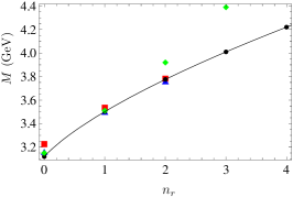
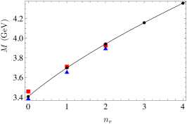
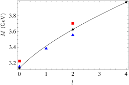
Figure 1: The radial and orbital Regge trajectories for the $(cc)$ diquark. (a) Radial Regge trajectory for the diquark $\{cc\}^{\bar{3}_{c}}_{1^{3}s_{1}}$ state. (b) Radial Regge trajectory for the diquark $\{cc\}^{\bar{3}_{c}}_{1^{1}p_{1}}$ state. (c) Orbital Regge trajectory for the $\{cc\}^{\bar{3}_{c}}_{1^{3}s_{1}}$ state. The data for the red filled squares are from EFMG or FG. The data for the blue filled triangles are from GKLO. The data for the green diamonds are from GAR. The black lines and the black dots are our results. The data are listed in Tables 1 and 2.

III.2 Regge trajectories for the $(cc)$ diquark

By using Eq. (1) with (10), (11) and (III.1) [$\sigma^{\prime}=\sigma$ and $\epsilon_{c}=C$ for mesons] to fit the radial $J/\psi(1S)$ and $h_{c}(1P)$ Regge trajectories, we have $c_{0n_{r}}=0.205$ and $c_{0n_{r}}=0.907$, respectively. Fitting the orbital $\eta_{c}(1S)$ and $J/\psi(1S)$ Regge trajectories gives $c_{0l}=0.188$ and $c_{0l}=0.337$, respectively. To calculated the masses of the $\{cc\}^{{\bar{3}_{c}}}_{1^{3}d_{1}}$ and $\{cc\}^{{\bar{3}_{c}}}_{1^{3}d_{2}}$ states, we fit the orbital $\chi_{c0}(1P)$ and $\chi_{c1}(1P)$ Regge trajectories and obtain $c_{0l}=1.016$, $c_{0l}=1.231$, respectively.

Table 1: Comparison of the theoretical values (in GeV) for the diquark $(cc)$. The data from Ref. Gershtein:2000nx are without spin-dependent splittings. $n=n_{r}+1$, $n_{r}=0,1,\cdots$. $n_{r}$ is the radial quantum number. $s$ is the total spin of two quarks, $l$ is the orbital quantum number and $j$ is the spin of diquark. The acronyms are from the initial letters of the last name of authors.

State ($n^{2s+1}l_{j}$)	EFGM Ebert:2002ig	GKLO Gershtein:2000nx	GAR Gutierrez-Guerrero:2021fuj	Our results
$1^{3}s_{1}$	3.226	3.16	3.15	3.12
$2^{3}s_{1}$	3.535	3.50	3.51	3.50
$3^{3}s_{1}$	3.782	3.76	3.92	3.78
$4^{3}s_{1}$			4.39	4.01
$5^{3}s_{1}$				4.22
$1^{1}p_{1}$	3.460	3.39		3.41
$2^{1}p_{1}$	3.712	3.66		3.70
$3^{1}p_{1}$	3.928	3.90		3.94
$4^{1}p_{1}$				4.16
$5^{1}p_{1}$				4.36

Table 2: The theoretical values (in GeV) for the $(cc)$ diquark. The data from Ref. Gershtein:2000nx are without spin-dependent splittings. $\times$ denotes the nonexistent states. The acronyms are from the initial letters of the last name of authors.

State ($n^{2s+1}l_{j}$)	FG Faustov:2021qqf	GKLO Gershtein:2000nx	Our results
$1^{3}s_{1}$	3.226	3.16	3.14
$1^{3}p_{2}$		3.39	3.42($\times$)
$1^{3}d_{3}$	3.704	3.56	3.63
$1^{3}f_{4}$			3.81($\times$)
$1^{3}g_{5}$			3.97

Substituting the values in Eq. (III.1) and the obtained $c_{0x}$ into (10) and (11), Eq. (1) is determined [$\sigma^{\prime}=\sigma/2$ and $\epsilon_{c}=C/2$ for diquarks]. We use (1) to calculate the masses of diquark $(cc)$, which are listed in Tables 1, 2 and 7. As we fit the parameter $c_{0x}$, the spin-dependent effects are considered in fact. For example, we fit the orbital $J/\psi(1S)$ Regge trajectory, then the obtained ${c_{0l}}$ is used for the orbital $\{cc\}^{{\bar{3}_{c}}}_{1^{3}s_{1}}$ Regge trajectory. Here, we do not consider the ${}^{3}(j-1)_{j}-^{3}(j+1)_{j}$ mixing of diquarks which is similar to the mixing of different wave states of charmonium and bottomonium Eichten:2007qx . The mass of state $\{cc\}^{{\bar{3}_{c}}}_{2^{3}s_{1}}$ is estimated by using the radial $\{cc\}^{{\bar{3}_{c}}}_{1^{3}s_{1}}$ Regge trajectory, $m(\{cc\}^{{\bar{3}_{c}}}_{2^{3}s_{1}})=3.535$ GeV. The mass of state $\{cc\}^{{\bar{3}_{c}}}_{1^{3}d_{1}}$ is computed by using the orbital $\{cc\}^{{\bar{3}_{c}}}_{1^{3}p_{0}}$ Regge trajectory, $m(\{cc\}^{{\bar{3}_{c}}}_{1^{3}d_{1}})=3.56$ GeV.

The spectrum from GKLO Gershtein:2000nx is without spin-dependent splittings. The symbol $\times$ in Table 2 denotes the nonexisting states according to the Pauli exclusion principle; see the Appendix for more details.

Our results obtained by the Regge trajectory approach are consistent with other theoretical results, as shown in Tables 1, 2, and 7 and Fig. 1. As depicted in Fig. 1, our results are in agreement with EFGM Ebert:2002ig and GKLOGershtein:2000nx . The behavior of Regge trajectory is different from the data from GAR Gutierrez-Guerrero:2021fuj ; see Fig. 1.

III.3 Regge trajectories for the $(bb)$ diquark

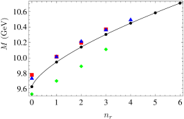
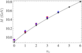
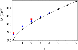
Figure 2: The radial and orbital Regge trajectories for the $(bb)$ diquark. (a) Radial Regge trajectory for the $\{bb\}^{\bar{3}_{c}}_{1^{3}s_{1}}$ state. (b) Radial Regge trajectory for the $\{bb\}^{\bar{3}_{c}}_{1^{1}p_{1}}$ state. (c) Orbital Regge trajectory for the $\{bb\}^{\bar{3}_{c}}_{1^{3}s_{1}}$ state. The data for the red filled squares are from EFGM or FG. The data for the blue filled triangles are from GKLO. The data for the green diamonds are from GAR. The black lines and the black dots are our results. The data are listed in Tables 3 and 4.

By using Eq. (1) in conjunction with (10), (11) and (III.1) to fit the radial $\Upsilon(1S)$ and $h_{b}(1P)$ Regge trajectories, we have $c_{0n_{r}}=0.01$ and $c_{0n_{r}}=0.795$, respectively. Fitting the orbital $\eta_{b}(1S)$ and $\Upsilon(1S)$ Regge trajectories gives $c_{0l}=0$, $c_{0l}=0.001$, respectively. To calculate the masses of the $\{bb\}^{{\bar{3}_{c}}}_{1^{3}d_{1}}$ and $\{bb\}^{{\bar{3}_{c}}}_{1^{3}d_{2}}$ states, we fit the orbital $\chi_{b0}(1P)$ Regge trajectory and the radial $\chi_{b1}(1P)$ Regge trajectory and obtain $c_{0l}=0.942$, $c_{0n_{r}}=0.786$, respectively.

Using Eq. (1) with (10), (11), (III.1) and the obtained $c_{0x}$, we calculate the masses of diquark $(bb)$. The masses are listed in Tables 3, 4 and 7. The corresponding Regge trajectories are in Fig. 2. As shown in Tables 3, 4, and 7 and Fig. 2, our results are in accordance with other theoretical results.

Similar to the $(cc)$ diquark case, we do not consider the ${}^{3}(j-1)_{j}-^{3}(j+1)_{j}$ mixing of $(bb)$ diquarks. The mass of state $\{bb\}^{{\bar{3}_{c}}}_{2^{3}s_{1}}$ is estimated by using the radial $\{bb\}^{{\bar{3}_{c}}}_{1^{3}s_{1}}$ Regge trajectory, $m(\{bb\}^{{\bar{3}_{c}}}_{2^{3}s_{1}})=10.015$ GeV. The mass of state $\{bb\}^{{\bar{3}_{c}}}_{1^{3}d_{1}}$ is computed by using the orbital $\{bb\}^{{\bar{3}_{c}}}_{1^{3}p_{0}}$ Regge trajectory, $m(\{bb\}^{{\bar{3}_{c}}}_{1^{3}d_{1}})=10.02$ GeV.

Table 3: Same as Table 1 except for the diquark $(bb)$.

State ($n^{2s+1}l_{j}$)	EFGM Ebert:2002ig	GAR Gutierrez-Guerrero:2021fuj	GKLO Gershtein:2000nx	Our results
$1^{3}s_{1}$	9.778	9.53	9.74	9.63
$2^{3}s_{1}$	10.015	9.70	10.02	9.95
$3^{3}s_{1}$	10.196	9.89	10.22	10.14
$4^{3}s_{1}$	10.369	10.11	10.37	10.30
$5^{3}s_{1}$			10.50	10.45
$6^{3}s_{1}$				10.58
$1^{1}p_{1}$	9.944		9.95	9.90
$2^{1}p_{1}$	10.132		10.15	10.10
$3^{1}p_{1}$	10.305		10.31	10.27
$4^{1}p_{1}$	10.453		10.45	10.42
$5^{1}p_{1}$			10.58	10.56
$6^{1}p_{1}$				10.68

Table 4: Same as Table 2 except for the diquark $(bb)$.

State ($n^{2s+1}l_{j}$)	FG Faustov:2021qqf	GKLO Gershtein:2000nx	Our results
$1^{3}s_{1}$	9.778	9.74	9.61
$1^{3}p_{2}$		9.95	9.87($\times$)
$1^{3}d_{3}$	10.123	10.08	10.03
$1^{3}f_{4}$		10.19	10.15($\times$)
$1^{3}g_{5}$		10.28	10.27
$1^{3}h_{6}$		10.37	10.38($\times$)

III.4 Regge trajectories for the $(bc)$ diquark

Table 5: Same as Table 1 except for the diquark $(bc)$.

State ($n^{2s+1}l_{j}$)	GAR Gutierrez-Guerrero:2021fuj	GKLO Gershtein:2000nx	Our results
$1^{3}s_{1}$	6.38	6.48	6.42
$2^{3}s_{1}$	6.66	6.79	6.75
$3^{3}s_{1}$	6.97	7.01	6.99
$4^{3}s_{1}$	7.30		7.20
$5^{3}s_{1}$			7.38
$1^{1}s_{0}$	6.33	6.48	6.38
$2^{1}s_{0}$	6.60	6.79	6.73
$3^{1}s_{0}$	6.92	7.01	6.98
$4^{1}s_{0}$	7.25		7.18
$5^{1}s_{0}$			7.37
$1^{3}p_{0}$		6.69	6.64
$2^{3}p_{0}$		6.93	6.90
$3^{3}p_{0}$		7.13	7.12
$4^{3}p_{0}$			7.31
$5^{3}p_{0}$			7.48
$1^{3}d_{1}$		6.85	6.84
$2^{3}d_{1}$		7.05	7.07
$3^{3}d_{1}$			7.26
$4^{3}d_{1}$			7.44
$5^{3}d_{1}$			7.61

Table 6: Same as Table 2 except for the diquark $(bc)$.

State ($n^{2s+1}l_{j}$)	GKLO Gershtein:2000nx	Our results
$1^{1}s_{0}$	6.48	6.38
$1^{1}p_{1}$	6.69	6.65
$1^{1}d_{2}$	6.85	6.84
$1^{1}f_{3}$	6.97	7.00
$1^{1}g_{4}$	7.09	7.14
$1^{1}h_{5}$	7.19	7.28
$1^{3}s_{1}$	6.48	6.41
$1^{3}p_{2}$	6.69	6.67
$1^{3}d_{3}$	6.85	6.85
$1^{3}f_{4}$	6.97	7.01
$1^{3}g_{5}$	7.09	7.16
$1^{3}h_{6}$	7.19	7.29

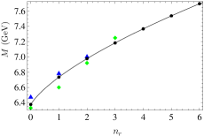
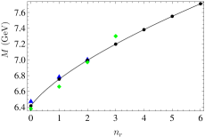
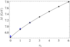
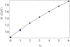
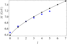
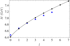
Figure 3: The radial and orbital Regge trajectories for the $(bc)$ diquark. (a), (b), (c) and (d) Radial Regge trajectory for the $\{bc\}^{\bar{3}_{c}}_{1^{3}s_{0}}$ state, the $\{bc\}^{\bar{3}_{c}}_{1^{3}s_{1}}$ state, the $\{bc\}^{\bar{3}_{c}}_{1^{3}p_{0}}$ and the $\{bc\}^{\bar{3}_{c}}_{1^{3}d_{1}}$ state, respectively. (e) and (f) Orbital Regge trajectory for the $\{bc\}^{\bar{3}_{c}}_{1^{1}s_{0}}$ state and the $\{bc\}^{\bar{3}_{c}}_{1^{3}s_{1}}$ state, respectively. The data for the blue filled triangles are from GKLO. The data for the green diamonds are from GAR. The black lines and the black dots are our results. The data are listed in Tables 5 and 6.

Table 7: Comparison of theoretical predictions for the masses of the doubly heavy diquarks (in GeV).

$j^{P}$	Diquark	Our results	FG Faustov:2021qqf , FGS Faustov:2020qfm	GKLO Gershtein:2000nx	GPB Gutierrez-Guerrero:2021rsx	YCRS Yin:2021uom	F Ferretti:2019zyh
$0^{+}$	$[bc]^{{\bar{3}_{c}}}_{1^{1}s_{0}}$	6.38	6.519	6.48	6.35	6.48	6.599
$0^{-}$	$[bc]^{{\bar{3}_{c}}}_{1^{3}p_{0}}$	6.64		6.69	6.47	6.62
$1^{+}$	$\{cc\}^{{\bar{3}_{c}}}_{1^{3}s_{1}}$	3.14	3.226	3.16	3.22	3.30	3.329
	$\{cc\}^{{\bar{3}_{c}}}_{1^{3}d_{1}}$	3.56	3.704	3.56
	$\{bb\}^{{\bar{3}_{c}}}_{1^{3}s_{1}}$	9.63	9.778	9.74	9.44	9.68	9.845
	$\{bb\}^{{\bar{3}_{c}}}_{1^{3}d_{1}}$	10.02	10.123	10.08
	$\{bc\}^{{\bar{3}_{c}}}_{1^{3}s_{1}}$	6.42	6.526	6.48	6.35	6.50	6.611
	$\{bc\}^{{\bar{3}_{c}}}_{1^{3}d_{1}}$	6.84		6.85
$1^{-}$	$\{cc\}^{{\bar{3}_{c}}}_{1^{1}p_{1}}$	3.41	3.460	3.39	3.42
	$\{bb\}^{{\bar{3}_{c}}}_{1^{1}p_{1}}$	9.90	9.944	9.95	9.53
	$\{bc\}^{{\bar{3}_{c}}}_{1^{1}p_{1}}$	6.65		6.69	6.50

Although the excited states of the diquark $(bc)$ are unstable under the emission of soft gluons Gershtein:2000nx , the authors provide the spectra of diquark $(bc)$. We obtain the orbital and radial diquark $(bc)$ Regge trajectories by fitting the corresponding $B_{c}$ Regge trajectories. Simultaneously, the spectra of diquark $(bc)$ are calculated.

There are scarce experimental data for the excited $B_{c}$ mesons. For the $B_{c}^{+}$ and $B_{c}(2S)^{\pm}$, the masses are from ParticleDataGroup:2022pth while the theoretically predicted masses for other states are from Ref. Godfrey:2004ya .

Because b quark and c quark are not identical, both $\{bc\}$ and $[bc]$ exist and there are more Regge trajectories for diquark $(bc)$ than that for diquarks $(cc)$ and $(bb)$. By using Eq. (1) with (10), (11) and (III.1) to fit the radial Regge trajectories for the $B_{c}(1^{1}S_{0})$, $B_{c}(1^{3}S_{1})$, $B_{c}(1^{3}P_{0})$, $B_{c}(1^{3}D_{1})$, we have $c_{0n_{r}}=0.107,\;0.182,\;0.783,\;1.516$, respectively. Fitting the orbital Regge trajectories for the $B_{c}(1^{1}S_{0})$ and $B_{c}(1^{3}S_{1})$ gives $c_{0l}=0.169$ and $c_{0l}=0.257$, respectively.

Using Eq. (1) with (10), (11), (III.1) and the obtained $c_{0x}$, we calculate the masses of diquark $(bc)$. The masses are listed in Tables 5, 6 and 7. The corresponding Regge trajectories are in Fig. 3. As shown in Tables 5, 6, 7 and Fig. 3, our results are in accordance with other theoretical results.

In the $B_{c}$ meson case, there is mixing of the singlet and triplet states; for example, the P-wave states are linear combinations of ${}^{3}P_{1}$ and ${}^{1}P_{1}$ which can be described by $P^{\prime}=^{1}P_{1}\,cos\theta+^{3}P_{1}\,sin\theta$, $P=-^{1}P_{1}\,sin\theta+^{3}P_{1}\,cos\theta$ Godfrey:2004ya . In the diquark $(bc)$ case, there will be the ${}^{3}l_{l}-^{1}l_{l}$ mixing via the spin-orbit interaction Ebert:2002ig or some other mechanism. We do not consider this kind of mixed state here.

IV Conclusions

As shown in Sec. III, the spectra of the doubly heavy diquarks $(cc)$, $(bb)$, and $(bc)$ obtained by the Regge trajectory approach agree with other theoretical results. This demonstrates that the Regge trajectory relation (1), which is appropriate for mesons, baryons and tetraquarks, is suitable for the doubly heavy diquarks.

We present a method to determine the parameters in the diquark Regge trajectories. Once the parameters are determined, the Regge trajectory becomes a new and very simple approach for estimating the spectra of diquarks. By employing (1) with (10) and (11) to fit the meson Regge trajectories, we can obtain values of the universal parameters. By fitting a chosen meson Regge trajectory, $c_{0x}$ is calculated. After all parameters are computed, the diquark Regge trajectory is definite and the spectra of diquarks can be estimated.

The diquark Regge trajectory is expected to provide a simple method to investigate easily the $\rho-$mode excitations of baryons, tetraquarks and pentaquarks in the diquark picture.

Appendix A States of diquarks

The diquark $(qq^{\prime})$ can be in two different $SU_{c}(3)$ configurations, $\bar{3}_{c}$ and $6_{c}$. The diquark’s color wave function is a superposition of these two different $SU_{c}(3)$ color representations Anwar:2018sol ; Barabanov:2020jvn :

$$\xi_{color}=a\xi_{\bar{3}_{c}}+b\xi_{6_{c}},\;a^{2}+b^{2}=1.$$ (18)

In the diquark picture, the diquark should be in $\bar{3}_{c}$ with a quark in $3_{c}$ to form a colorless baryon. In the tetraquark case, a diquark in $\bar{3}_{c}$ or in $6_{c}$ together with an antidiquark in $3_{c}$ or in $\bar{6}_{c}$ forms a color singlet.

The total wave function for the diquarks $(qq^{\prime})$ is written as

$$\psi_{D}=\xi_{color}\otimes\eta_{flavor}\otimes\chi_{spin}\otimes\phi_{space},$$ (19)

where $\xi_{color}$, $\eta_{flavor}$, $\chi_{spin}$ and $\phi_{space}$ are the color, flavor, spin and spatial wave functions, respectively, see Table 8. If the quarks are of the same flavor $q=q^{\prime}$, the diquark wave function $\psi_{D}$ must be completely antisymmetric to satisfy the Pauli principle. When a diquark contains light quarks with flavors u,d,s, the overall state $\psi_{D}$ must also be antisymmetric because strong interactions do not distinguish the flavor of u,d,s Esposito:2016noz .

Table 8: Wave functions are symmetric (S) or antisymmetric (A). The flavor wave function for the diquark $(qq^{\prime})$ can be symmetric $\{qq^{\prime}\}$ or antisymmetric $[qq^{\prime}]$. $s$ stands for the total spin of two quarks. $n=0,1,2,\cdots$.

	$\xi_{color}$	$\eta_{flavor}$	$\chi_{spin}$	$\phi_{space}$
S	$6_{c}$	$\{qq^{\prime}\}$	$s=1$	$l=2n$
A	$\bar{3}_{c}$	$[qq^{\prime}]$	$s=0$	$l=2n+1$

In the color space, the color wave function can be analyzed by employing the $SU_{c}(3)$ group theory

$$3_{c}\otimes 3_{c}={\bar{3}_{c}}\oplus 6_{c}.$$ (20)

The color wave functions for the diquark read as

$$\xi_{\bar{3}_{c}}=|(qq^{\prime})^{\bar{3}_{c}}\rangle,\quad\xi_{6_{c}}=|(qq^{\prime})^{6_{c}}\rangle.$$ (21)

The spin triplets are symmetric while the spin singlet is antisymmetric. The spin wave functions read as

$$\chi_{S}=|(qq^{\prime})_{1}\rangle,\quad\chi_{A}=|(qq^{\prime})_{0}\rangle.$$ (22)

If $q{\neq}q^{\prime}$, the flavor wave functions can be written in the symmetric and the antisymmetric form as

$$\eta_{S} =\{qq^{\prime}\}=\frac{1}{\sqrt{2}}(qq^{\prime}+q^{\prime}q),$$

$$\eta_{A} =[qq^{\prime}]=\frac{1}{\sqrt{2}}(qq^{\prime}-q^{\prime}q)$$ (23)

while

$$\eta_{flavor}=\eta_{S}=\{qq^{\prime}\}=qq$$ (24)

if $q=q^{\prime}$.

Since quarks have the same intrinsic parities, the overall parity is

$$P((qq^{\prime}))=(-1)^{l},$$ (25)

where $l$ is the symmetry of the orbital wave function $\phi_{space}$.

Table 9: The completely antisymmetric states for the diquarks in $\bar{3}_{c}$ and in $6_{c}$. $j$ is the spin of the diquark $(qq^{\prime})$, $s$ denotes the total spin of two quarks, $l$ represents the orbital angular momentum. $n=n_{r}+1$, $n_{r}$ is the radial quantum number, $n_{r}=0,1,2,\cdots$.

Spin of diquark	Parity	Wave state	Configuration
( $j$ )	$(j^{P})$	$(n^{2s+1}l_{j})$
j=0	$0^{+}$	$n^{1}s_{0}$	$[qq^{\prime}]^{{\bar{3}_{c}}}_{n^{1}s_{0}}$,  $\{qq^{\prime}\}^{{6_{c}}}_{n^{1}s_{0}}$
	$0^{-}$	$n^{3}p_{0}$	$[qq^{\prime}]^{{\bar{3}_{c}}}_{n^{3}p_{0}}$,  $\{qq^{\prime}\}^{{6_{c}}}_{n^{3}p_{0}}$
j=1	$1^{+}$	$n^{3}s_{1}$, $n^{3}d_{1}$	$\{qq^{\prime}\}^{{\bar{3}_{c}}}_{n^{3}s_{1}}$,  $\{qq^{\prime}\}^{{\bar{3}_{c}}}_{n^{3}d_{1}}$,  $[qq^{\prime}]^{6_{c}}_{n^{3}s_{1}}$,  $[qq^{\prime}]^{{6_{c}}}_{n^{3}d_{1}}$
	$1^{-}$	$n^{1}p_{1}$, $n^{3}p_{1}$	$\{qq^{\prime}\}^{{\bar{3}_{c}}}_{n^{1}p_{1}}$,  $[qq^{\prime}]^{{\bar{3}_{c}}}_{n^{3}p_{1}}$,   $[qq^{\prime}]^{6_{c}}_{n^{1}p_{1}}$,  $\{qq^{\prime}\}^{6_{c}}_{n^{3}p_{1}}$
j=2	$2^{+}$	$n^{1}d_{2}$, $n^{3}d_{2}$	$[qq^{\prime}]^{{\bar{3}_{c}}}_{n^{1}d_{2}}$,  $\{qq^{\prime}\}^{{\bar{3}_{c}}}_{n^{3}d_{2}}$,  $\{qq^{\prime}\}^{6_{c}}_{n^{1}d_{2}}$,  $[qq^{\prime}]^{6_{c}}_{n^{3}d_{2}}$
	$2^{-}$	$n^{3}p_{2}$, $n^{3}f_{2}$	$[qq^{\prime}]^{{\bar{3}_{c}}}_{n^{3}p_{2}}$,  $[qq^{\prime}]^{{\bar{3}_{c}}}_{n^{3}f_{2}}$,  $\{qq^{\prime}\}^{6_{c}}_{n^{3}p_{2}}$,  $\{qq^{\prime}\}^{6_{c}}_{n^{3}f_{2}}$
$\cdots$	$\cdots$	$\cdots$	$\cdots$

For the diquarks composed of two identical quarks, the antisymmetric flavor wave function does not exist; therefore, the states in the $[qq]$ configuration disappear in Table 9. From Table 9, we can easily read the possible mixing of different states. For example, for the diquarks composed of different quarks, the $1^{+}$ state can be a mixture of the S-wave state and D-wave state, and the mixture of the $\bar{3}_{c}$ state and $6_{c}$ state.

References

- (1) M. Gell-Mann, Phys. Lett. 8, 214-215 (1964)
- (2) D. B. Lichtenberg and L. J. Tassie, Phys. Rev. 155, 1601-1606 (1967)
- (3) M. Anselmino, E. Predazzi, S. Ekelin, S. Fredriksson and D. B. Lichtenberg, Rev. Mod. Phys. 65, 1199-1234 (1993)
- (4) F. Wilczek, [arXiv:hep-ph/0409168 [hep-ph]].
- (5) M. Y. Barabanov, M. A. Bedolla, W. K. Brooks, G. D. Cates, C. Chen, Y. Chen, E. Cisbani, M. Ding, G. Eichmann and R. Ent, et al. Prog. Part. Nucl. Phys. 116, 103835 (2021) [arXiv:2008.07630 [hep-ph]].
- (6) A. Selem and F. Wilczek, [arXiv:hep-ph/0602128 [hep-ph]].
- (7) R. L. Jaffe and F. Wilczek, Phys. Rev. Lett. 91, 232003 (2003) [arXiv:hep-ph/0307341 [hep-ph]].
- (8) R. L. Jaffe, Phys. Rept. 409, 1-45 (2005) [arXiv:hep-ph/0409065 [hep-ph]].
- (9) M. Ida and R. Kobayashi, Prog. Theor. Phys. 36 (1966), 846
- (10) Y. R. Liu, H. X. Chen, W. Chen, X. Liu and S. L. Zhu, Prog. Part. Nucl. Phys. 107 (2019), 237-320 [arXiv:1903.11976 [hep-ph]].
- (11) A. Esposito, A. Pilloni and A. D. Polosa, Phys. Rept. 668 (2017), 1-97 [arXiv:1611.07920 [hep-ph]].
- (12) R. L. Jaffe, Phys. Rev. D 15 (1977), 267
- (13) R. F. Lebed, Phys. Lett. B 749 (2015), 454-457 [arXiv:1507.05867 [hep-ph]].
- (14) S. L. Olsen, T. Skwarnicki and D. Zieminska, Rev. Mod. Phys. 90 (2018) no.1, 015003 [arXiv:1708.04012 [hep-ph]].
- (15) F. K. Guo, X. H. Liu and S. Sakai, Prog. Part. Nucl. Phys. 112 (2020), 103757 [arXiv:1912.07030 [hep-ph]].
- (16) S. S. Gershtein, V. V. Kiselev, A. K. Likhoded and A. I. Onishchenko, Phys. Rev. D 62, 054021 (2000)
- (17) D. Ebert, R. N. Faustov, V. O. Galkin and A. P. Martynenko, Phys. Rev. D 66, 014008 (2002) [arXiv:hep-ph/0201217 [hep-ph]].
- (18) L. X. Gutierrez-Guerrero, J. Alfaro and A. Raya, Int. J. Mod. Phys. A 36, no.24, 2150171 (2021) [arXiv:2108.12532 [hep-ph]].
- (19) L. X. Gutiérrez-Guerrero, G. Paredes-Torres and A. Bashir, Phys. Rev. D 104, no.9, 094013 (2021) [arXiv:2109.09058 [hep-ph]].
- (20) P. L. Yin, Z. F. Cui, C. D. Roberts and J. Segovia, Eur. Phys. J. C 81, no.4, 327 (2021) [arXiv:2102.12568 [hep-ph]].
- (21) Q. Li, C. H. Chang, S. X. Qin and G. L. Wang, Chin. Phys. C 44, no.1, 013102 (2020) [arXiv:1903.02282 [hep-ph]].
- (22) Y. M. Yu, H. W. Ke, Y. B. Ding, X. H. Guo, H. Y. Jin, X. Q. Li, P. N. Shen and G. L. Wang, Commun. Theor. Phys. 46, 1031-1039 (2006) [arXiv:hep-ph/0602077 [hep-ph]].
- (23) Z. G. Wang, S. L. Wan and W. M. Yang, Commun. Theor. Phys. 47, 287-292 (2007) [arXiv:hep-ph/0506035 [hep-ph]].
- (24) R. T. Cahill, C. D. Roberts and J. Praschifka, Phys. Rev. D 36, 2804 (1987)
- (25) P. Maris, Few Body Syst. 32, 41-52 (2002) [arXiv:nucl-th/0204020 [nucl-th]].
- (26) Q. F. Lü, K. L. Wang, L. Y. Xiao and X. H. Zhong, Phys. Rev. D 96, no.11, 114006 (2017) [arXiv:1708.04468 [hep-ph]].
- (27) J. Ferretti, Few Body Syst. 60, no.1, 17 (2019)
- (28) M. Hess, F. Karsch, E. Laermann and I. Wetzorke, Phys. Rev. D 58, 111502 (1998) [arXiv:hep-lat/9804023 [hep-lat]].
- (29) T. Regge, Nuovo Cim. 14, 951 (1959)
- (30) G. F. Chew and S. C. Frautschi, Phys. Rev. Lett. 8, 41 (1962)
- (31) C. Lovelace, Phys. Lett. 28B, 264 (1968)
- (32) M. Ademollo, G. Veneziano and S. Weinberg, Phys. Rev. Lett. 22, 83 (1969)
- (33) P. D. B. Collins, Phys. Rept. 1, 103 (1971)
- (34) A. C. Irving and R. P. Worden, Phys. Rept. 34, 117 (1977)
- (35) Y. Nambu, Phys. Lett. B 80, 372 (1979)
- (36) S. Filipponi, Y. Srivastava, Phys. Rev. D 58, 016003 (1998). arXiv:hep-ph/9712204
- (37) A. Inopin and G. S. Sharov, Phys. Rev. D 63, 054023 (2001). arXiv: hep-ph/9905499.
- (38) M. M. Brisudova, L. Burakovsky and T. Goldman, Phys. Rev. D 61, 054013 (2000). arXiv:hep-ph/9906293
- (39) A. V. Anisovich, V. V. Anisovich and A. V. Sarantsev, Phys. Rev. D 62, 051502 (2000) [arXiv:hep-ph/0003113 [hep-ph]].
- (40) F. Brau, Phys. Rev. D 62, 014005 (2000). arXiv:hep-ph/0412170
- (41) M. Baker and R. Steinke, Phys. Rev. D 65, 094042 (2002). arXiv:hep-th/0201169
- (42) S. J. Brodsky, Eur. Phys. J. A 31, 638 (2007). arXiv:hep-ph/0610115
- (43) H. Forkel, M. Beyer and T. Frederico, JHEP 0707, 077 (2007). arXiv:hep-ph/0705.1857
- (44) X. H. Guo, K. W. Wei and X. H. Wu, Phys. Rev. D 78, 056005 (2008). arXiv:hep-ph/0809.1702
- (45) D. Ebert, R. N. Faustov and V. O. Galkin, Phys. Rev. D 79, 114029 (2009) [arXiv:0903.5183 [hep-ph]].
- (46) P. Masjuan, E. Ruiz Arriola and W. Broniowski, Phys. Rev. D 85, 094006 (2012) [arXiv:1203.4782 [hep-ph]].
- (47) B. Chen, K. W. Wei and A. Zhang, Eur. Phys. J. A 51, 82 (2015) [arXiv:1406.6561 [hep-ph]].
- (48) S. S. Afonin and I. V. Pusenkov, Phys. Rev. D 90, no.9, 094020 (2014) [arXiv:1411.2390 [hep-ph]].
- (49) J. Sonnenschein and D. Weissman, Eur. Phys. J. C 79, no.4, 326 (2019) [arXiv:1812.01619 [hep-ph]].
- (50) A. M. Badalian and B. L. G. Bakker, Phys. Rev. D 100, no.5, 054036 (2019) [arXiv:1902.09174 [hep-ph]].
- (51) M. A. Martin Contreras and A. Vega, Phys. Rev. D 102, no.4, 046007 (2020) [arXiv:2004.10286 [hep-ph]].
- (52) J. K. Chen, Nucl. Phys. B 983, 115911 (2022) [arXiv:2203.02981 [hep-ph]].
- (53) X. C. Feng and K. W. Wei, [arXiv:2303.10332 [hep-ph]].
- (54) J. K. Chen, [arXiv:2302.05926 [hep-ph]].
- (55) J. K. Chen, [arXiv:2302.06794 [hep-ph]].
- (56) The Regge trajectories are commenly plotted in the plane or in the plane, where . For simplicity, the figures plotted in the plane, in the plane and in the plane are also called the Regge trajectories.
- (57) M. Baldicchi, A. V. Nesterenko, G. M. Prosperi, D. V. Shirkov and C. Simolo, Phys. Rev. Lett. 99 (2007), 242001 [arXiv:0705.0329 [hep-ph]].
- (58) M. Baldicchi, A. V. Nesterenko, G. M. Prosperi and C. Simolo, Phys. Rev. D 77 (2008), 034013 [arXiv:0705.1695 [hep-ph]].
- (59) N. Brambilla, E. Montaldi and G. M. Prosperi, Phys. Rev. D 54 (1996), 3506-3525 [arXiv:hep-ph/9504229 [hep-ph]].
- (60) J. K. Chen, Acta Phys. Pol. B 47, 1155 (2016)
- (61) J. K. Chen, Rom. J. Phys. 62, 119 (2017)
- (62) J. K. Chen, Eur. Phys. J. C 78, no.3, 235 (2018)
- (63) J. K. Chen, Phys. Lett. B 786, 477-484 (2018) [arXiv:1807.11003 [hep-ph]].
- (64) J. K. Chen, Eur. Phys. J. C 78 (2018) no.8, 648
- (65) J. K. Chen, Eur. Phys. J. A 57, 238 (2021) [arXiv:2102.07993 [hep-ph]].
- (66) X. Z. Weng, W. Z. Deng and S. L. Zhu, Chin. Phys. C 46, no.1, 013102 (2022) [arXiv:2108.07242 [hep-ph]].
- (67) M. Praszalowicz, Phys. Rev. D 106, no.11, 114005 (2022) [arXiv:2208.08602 [hep-ph]].
- (68) E. Eichten, K. Gottfried, T. Kinoshita, J. B. Kogut, K. D. Lane and T. M. Yan, Phys. Rev. Lett. 34, 369-372 (1975) [erratum: Phys. Rev. Lett. 36, 1276 (1976)]
- (69) W. Lucha, F. F. Schoberl and D. Gromes, Phys. Rept. 200, 127-240 (1991)
- (70) D. Gromes, Z. Phys. C 11, 147 (1981)
- (71) F. Brau, Phys. Rev. D 62, 014005 (2000) [arXiv:hep-ph/0412170 [hep-ph]].
- (72) S. Tomonaga, Quantum Mechanics, Volume I: Old Quantum Theory (North-Holland Publishing Company, Amsterdam, 1962)
- (73) I.S. Gradshteyn and I.M. Ryzhik, Table of Integrals, Series, and Products, corrected and, enlarged edition (Academic Press, New York, 1980)
- (74) R. L. Workman et al. [Particle Data Group], PTEP 2022 (2022), 083C01
- (75) J. Sonnenschein and D. Weissman, JHEP 08, 013 (2014) [arXiv:1402.5603 [hep-ph]].
- (76) R. N. Faustov and V. O. Galkin, Phys. Rev. D 105, no.1, 014013 (2022) [arXiv:2111.07702 [hep-ph]].
- (77) E. Eichten, S. Godfrey, H. Mahlke and J. L. Rosner, Rev. Mod. Phys. 80, 1161-1193 (2008) [arXiv:hep-ph/0701208 [hep-ph]].
- (78) S. Godfrey, Phys. Rev. D 70, 054017 (2004) [arXiv:hep-ph/0406228 [hep-ph]].
- (79) R. N. Faustov, V. O. Galkin and E. M. Savchenko, Phys. Rev. D 102, no.11, 114030 (2020) [arXiv:2009.13237 [hep-ph]].
- (80) M. N. Anwar, J. Ferretti and E. Santopinto, Phys. Rev. D 98, no.9, 094015 (2018) [arXiv:1805.06276 [hep-ph]].