KMT-2021-BLG-1150Lb: Microlensing planet detected through a densely covered planetary-caustic signal

Abstract

Aims. Recently, there have been reports of various types of degeneracies in the interpretation of planetary signals induced by planetary caustics. In this work, we check whether such degeneracies persist in the case of well-covered signals by analyzing the lensing event KMT-2021-BLG-1150, for which the light curve exhibits a densely and continuously covered short-term anomaly.

Methods. In order to identify degenerate solutions, we thoroughly investigate the parameter space by conducting dense grid searches for the lensing parameters. We then check the severity of the degeneracy among the identified solutions.

Results. We identify a pair of planetary solutions resulting from the well-known inner-outer degeneracy, and find that interpreting the anomaly is not subject to any degeneracy other than the inner-outer degeneracy. The measured parameters of the planet separation (normalized to the Einstein radius) and mass ratio between the lens components are $(s,q)_{\rm in}\sim(1.297,1.10\times 10^{-3})$ for the inner solution and $(s,q)_{\rm out}\sim(1.242,1.15\times 10^{-3})$ for the outer solution. According to a Bayesian estimation, the lens is a planetary system consisting of a planet with a mass $M_{\rm p}=0.88^{+0.38}_{-0.36}\leavevmode\nobreak\ M_{\rm J}$ and its host with a mass $M_{\rm h}=0.73^{+0.32}_{-0.30}\leavevmode\nobreak\ M_{\odot}$ lying toward the Galactic center at a distance $D_{\rm L}=3.8^{+1.3}_{-1.2}$ kpc. By conducting analyses using mock data sets prepared to mimic those obtained with data gaps and under various observational cadences, it is found that gaps in data can result in various degenerate solutions, while the observational cadence does not pose a serious degeneracy problem as long as the anomaly feature can be delineated.

1 Introduction

The microlensing signal of a planet generally appears as a short-term anomaly to the lensing light curve produced by the host of the planet (Mao & Paczyński, 1991; Gould & Loeb, 1992). The planetary signal is produced when a source star approaches close to or passes over the lensing caustic induced by the planet. A planetary companion induces two sets of caustics, in which one tiny set forms near the host of the planetary system, and the other set forms in the region away from the host with a separation $\sim{\bf s}-1/{\bf s}$, where ${\bf s}$ denote the planet-host separation vector. The former and latter caustics are referred to as ”central” and ”planetary” caustics, respectively. Due to the caustic location, the planetary signal generated by the central caustic appears near the peak of a high-magnification event, while the signal produced by the planetary caustic can appear at any part of the lensing light curve.

In the early phase of the planetary microlensing experiments, the majority of microlensing planets were found from the observations of high-magnifications events, for example, OGLE-2005-BLG-071Lb (Udalski et al., 2005), OGLE-2005-BLG-169Lb (Gould et al., 2006), and MOA-2007-BLG-192Lb (Bennett et al., 2008). This was because the observational cadence of the microlensing surveys at that time was generally not high enough to detect short-term planetary signals, and thus planet searches were carried out in a survey+followup mode, in which survey groups mainly concentrated on event detections, and followup groups conducted high-cadence followup observations for a fraction of events found by the survey groups. In this observation mode, high-magnification events were important targets because the chance for the source stars of these events to pass the perturbation regions induced by the central caustics was very high and the time of the event peak could be predicted in advance for the preparation of followup observations (Griest & Safizadeh, 1998).

With the launch of high-cadence microlensing surveys in the 2010s, not only the total detection rate of microlensing planets but also the fraction of planets detected via the perturbations induced by planetary caustics have greatly increased, for example, KMT-2016-BLG-1105Lb, KMT-2017-BLG-1194Lb, and OGLE-2017-BLG-1806 (Zang et al., 2023), KMT-2018-BLG-0173Lb (Jung et al., 2022), KMT-2021-BLG-0712Lb and KMT-2021-BLG-0909Lb (Ryu et al., 2023). The total planet detection rate has increased because all lensing events can be densely monitored regardless of lensing magnifications without the need of extra followup observations. The rate of planet detections via the signals generated by planetary caustics has increased because all parts of lensing light curves can be monitored with moderately-high to very-high cadences.

The classic type of degeneracy in the interpretations of the signals induced by planetary caustics is the ”inner-outer” degeneracy, which was predicted by Gaudi & Gould (1997) even before the detection of the first microlensing planet OGLE 2003-BLG-235/MOA-2003-BLG-53Lb (Bond et al., 2004). This degeneracy is intrinsic in the sense that it arises due to the intrinsic similarity between the magnification patterns on the near (to the primary lens) and far sides of the planetary caustic, and thus the planetary signal resulting from the source trajectory passing on near side of the caustic would be similar to the signal resulting from the trajectory passing on the far side. The origins of this degeneracy have been further explored in Zhang et al. (2022).

As the number of planets detected from actually observed signals generated by planetary increases, various types of unexpected degeneracies have been reported. From the analysis of the planetary lensing event OGLE-2017-BLG-0173, Hwang et al. (2018) reported a new type of degeneracy between the solution in which the source fully enveloped the caustic and the other solution in which the source enveloped one side of the caustic. They also reported a degeneracy between the solution in which the light-curve perturbation was generated by a planetary caustic due to a ”close” planet and the one in which it was generated by a ”wide” planet. Here the terms ”close” and ”wide” refer to the cases in which the projected planet-host separation is less and greater than the radius of the Einstein ring ($\theta_{\rm E}$), respectively. From the analysis of the anomaly appearing in the planetary lensing event OGLE-2017-BLG-0373, Skowron et al. (2018) also reported multiple degeneracies that had not been known before. We note that these new types of degeneracies were identified from the analyses of partially covered planetary signals, and thus it is not yet clear whether these degeneracies persist in the interpretations of continuously covered signals.

In this paper, we present the analysis of the lensing event KMT-2021-BLG-1150, for which a short-term signal induced by a planetary caustic appears on the lensing light curve. Despite the short duration, the anomaly was densely and continuously covered including both the caustic entrance and exit, and thus the event provides an important test bed that enables one to check whether various types of recently-reported degeneracies persist even for well covered planetary signals.

We present the analysis according to the following organization. In Sect. 2, we describe the observations of the lensing event and the data acquired from the observations. We mention the characteristics of the lensing event and the anomaly appearing in the lensing light curve. In Sect. 3, we depict the detailed procedure of the analysis and present the results found from the analysis. In Sect. 4, we explain the source characterization procedure conducted to estimate the angular Einstein radius and present the measured value of $\theta_{\rm E}$. In Sect. 5, we detail the Bayesian analysis conducted to estimate the physical parameters of the planetary system and present the estimated parameters. In Sect. 6, we present the results of the test conducted using mock data sets prepared to mimic those obtained with data gaps and under various observational cadences. We summarize the results of the analysis and conclude in Sect. 7.

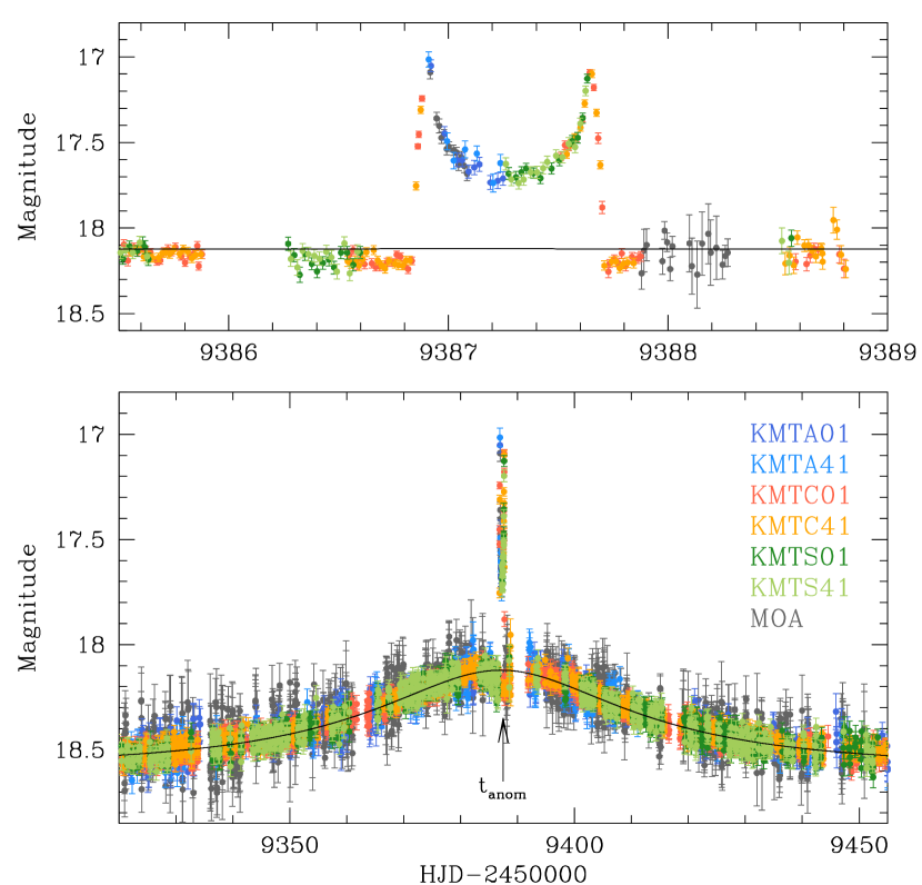
Figure 1: Light curve of KMT-2021-BLG-1150. The lower panel shows the whole view and the upper panel shows the zoom of the region around the anomaly. The curve drawn over the data point is a 1L1S model obtained by fitting the light curve excluding the data points around the anomaly.

2 Observations and data

The source of the microlensing event KMT-2021-BLG-1150 lies toward the Galactic bulge field at the equatorial coordinates $({\rm RA},{\rm DEC})_{\rm J2000}=($17:55:09.63, -31:18:47.99), which correspond to the Galactic coordinates $(l,b)=(-0^{\circ}\hskip-2.0pt.986,-2^{\circ}\hskip-2.0pt.989)$. The extinction toward the field is $A_{I}=1.50$, and the baseline $I$-band magnitude of the source is $I_{\rm base}=18.86$, as derived from the calibrated OGLE-III catalog (Szymański et al., 2011). The magnification of the source flux induced by lensing was first found by the EventFinder system (Kim et al., 2018) of the KMTNet group (Kim et al., 2016) on 2021 June 4, which corresponds to the abridged heliocentric Julian date ${\rm HJD}^{\prime}={\rm HJD}-2450000=9369.56$. On 2021 June 21, the event was independently found by the MOA group (Bond et al., 2001), who labeled the event as MOA-2021-BLG-197. Hereafter we refer to the event as KMT-2021-BLG-1150 following the convention of using the event ID reference of the first discovery group. The source lies in the KMTNet prime fields BLG01 and BLG41, toward which observations were conducted with a 0.5 hr cadence for each field and 0.25 hr in combination. The MOA observations were carried out at a similar cadence.

Observations by the KMTNet group were done utilizing the three identical 1.6 m telescopes that are globally distributed in the Southern Hemisphere at the Cerro Tololo Inter-American Observatory in Chile (KMTC), the South African Astronomical Observatory in South Africa (KMTS), and the Siding Spring Observatory in Australia (KMTA). The MOA group used the 1.8 m telescope located at the Mt. John Observatory in New Zealand. Images were acquired mainly in the $I$ band for the KMTNet survey and in the customized MOA-$R$ band for the MOA survey. For both surveys, subsets of images were taken in the $V$ band for the purpose of measuring the color of the source.

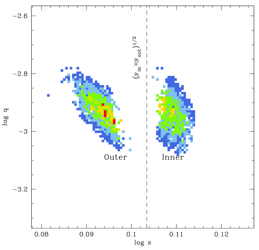
Figure 2: Map of $\Delta\chi^{2}$ in the space of the binary-lens parameters $s$ and $q$. The vertical dashed line indicates the geometric mean of $s_{\rm in}$ and $s_{\rm out}$, which represent the binary separations of the inner and outer solutions, respectively. The color coding is set to represent points with $\leq 1n\sigma$ (red), $\leq 2n\sigma$ (yellow), $\leq 3n\sigma$ (green), $\leq 4n\sigma$ (cyan) and, $\leq 5n\sigma$ (blue), where $n=3$.

Figure 1 shows the lensing light curve of KMT-2021-BLG-1150 constructed by combining the data from the KMTNet and MOA surveys. It displays a short-term anomaly appearing near the peak of the event. The curve drawn over the data points is the single-lens single-source (1L1S) model obtained by fitting the data excluding those around the anomaly. From the zoom-in view of the anomaly region presented in the top panel, it is found that the anomaly exhibits two caustic-crossing features at $t_{\rm c,1}\sim 9386.9$ (caustic entrance) and $t_{\rm c,2}\sim 9387.7$ (caustic exit) with a time gap $\Delta t_{\rm c}=t_{\rm c,2}-t_{\rm c,1}\sim 0.8$ day between the caustic features. Besides these caustic features, the anomaly exhibits negative deviations of $\sim 0.1$ mag level from the 1L1S model just before the caustic entrance and after the caustic exit. We note that all these anomaly features were densely resolved by the data from the combined high-cadence observations of the survey groups.

In the analysis of the event, we used the data prepared by reducing the images and conducting photometry of the source with the use of the pipelines of the individual groups. The pySIS pipeline of the KMTNet group was developed by Albrow et al. (2009), and that of the MOA survey was developed by Bond et al. (2001). Both pipelines commonly applied the difference image technique (Tomaney & Crotts, 1996; Alard & Lupton, 1998) that was developed for the optimal photometry of stars lying in very dense fields. Following the Yee et al. (2012) routine, we readjusted the error bars estimated by the pipelines so that the scatter of data is consistent with the error bars and the $\chi^{2}$ value per degree of freedom (dof) for each data becomes unity.

Table 1: Model parameters

Parameter	Inner	Outer
$\chi^{2}$/dof	$8139.7/8152$	$8133.4/8152$
$t_{0}$ (HJD′)	$9387.077\pm 0.055$	$9387.086\pm 0.055$
$u_{0}$	$0.502\pm 0.010$	$0.464\pm 0.010$
$t_{\rm E}$ (days)	$41.55\pm 0.58$	$43.75\pm 0.65$
$s$	$1.297\pm 0.005$	$1.242\pm 0.007$
$q$ ($10^{-3}$)	$1.10\pm 0.05$	$1.15\pm 0.05$
$\alpha$ (rad)	$4.703\pm 0.003$	$4.703\pm 0.003$
$\rho$ ($10^{-3}$)	$0.956\pm 0.015$	$0.899\pm 0.016$

3 Interpretation of the anomaly

The anomaly in the lensing light curve of KMT-2021-BLG-1150 is characterized by a near-peak caustic feature. Such an anomaly feature is known to be produced by 3 major channels. The first is the ”high-magnification” channel, in which an anomaly near the peak is produced when a source approaches close to the central caustic induced either by a planetary companion lying around the Einstein ring ($s\sim 1$) or a binary companion with a very small ($s\ll 1$) or large ($s\gg 1$) separation from the primary (Han & Hwang, 2009). The anomaly produced via this channel arises for a high-magnification event because the central caustic is very tiny (Chung et al., 2005), and thus the source should approach very close to the primary for the production of a near-peak anomaly. The second is the ”right-angle” channel, in which a near-peak anomaly is generated when a source passes the perturbation region around the caustic at an approximately right angle with respect to the planet-host axis, for example, KMT-2021-BLG-0748 (Ryu et al., 2022) and KMT-2021-BLG-1554 (Han et al., 2022). In this case, the anomaly can arise regardless of the peak magnification because the caustic can appear at any part around the Einstein ring. The third is the ”off-axis” channel, in which a near-peak anomaly is produced by the source passage through the anomaly region around the caustic lying away from the binary axis, for example, OGLE-2016-BLG-1266 (Albrow et al., 2018) and the off-axis solution of KMT-2018-BLG-1497 (Jung et al., 2022). Among these channels, the anomaly in KMT-2021-BLG-1150 is unlikely to be produced by the high-magnification channel because it appears when the magnification $A_{\rm anom}\sim 2.4$ is not very high.

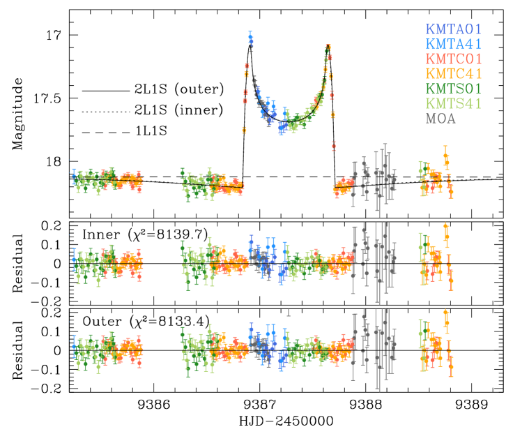
Figure 3: Enlarged view around the region of the anomaly. The dashed, dotted, and solid curves represent the models of the 1L1S, inner 2L1S, and outer 2L1S solutions, respectively. We note that the model curves of the inner and outer 2L1S solutions are so similar that it is difficult to resolve them with the given line width.

For the interpretation of the anomaly, we conducted modeling of the observed lensing light curve. In the modeling, we searched for a lensing solution representing a set of the lensing parameters that best described the observed anomaly. Considering that caustic features are produced by the multiplicity of a lens, we conducted a binary-lens single-source (2L1S) modeling. The lensing parameters of the 2L1S model include $(t_{0},u_{0},t_{\rm E},s,q,\alpha,\rho)$. The first three of these parameters describe the source approach to the lens, and they represent the time of the closest lens-source approach, the separation at that time, and the event time scale, respectively. The next three parameters describe the binarity of the lens, and the individual parameters denote the projected separation (scaled to $\theta_{\rm E}$) and mass ratio between the lens components, and the source trajectory angle defined as the angle between the source trajectory and the binary axis. The last parameter denotes the ratio of the angular source radius $\theta_{*}$ to the Einstein radius, that is, $\rho=\theta_{*}/\theta_{\rm E}$ (normalized source radius), and this parameters is needed to describe the deformation of the caustic-crossing features by finite-source effects.

Considering that various types of degeneracies had been reported from the recent analyses of microlensing planets detected through the signals generated by planetary caustics, we thoroughly investigated the parameter space to check all possible degenerate solutions. Figure 2 shows the $\Delta\chi^{2}$ map constructed by conducting dense grid searches for the binary-lens parameters $s$ and $q$. The map shows two distinct local solutions resulting from the inner-outer degeneracy with planetary parameters $(s,q)_{\rm in}\sim(1.297,1.10\times 10^{-3})$ for the inner solution and $(s,q)_{\rm out}\sim(1.242,1.15\times 10^{-3})$ for the outer solution. The degeneracy between the two solutions is fairly severe, although the outer solution is slightly preferred over the inner solution by $\Delta\chi^{2}=6.3$.

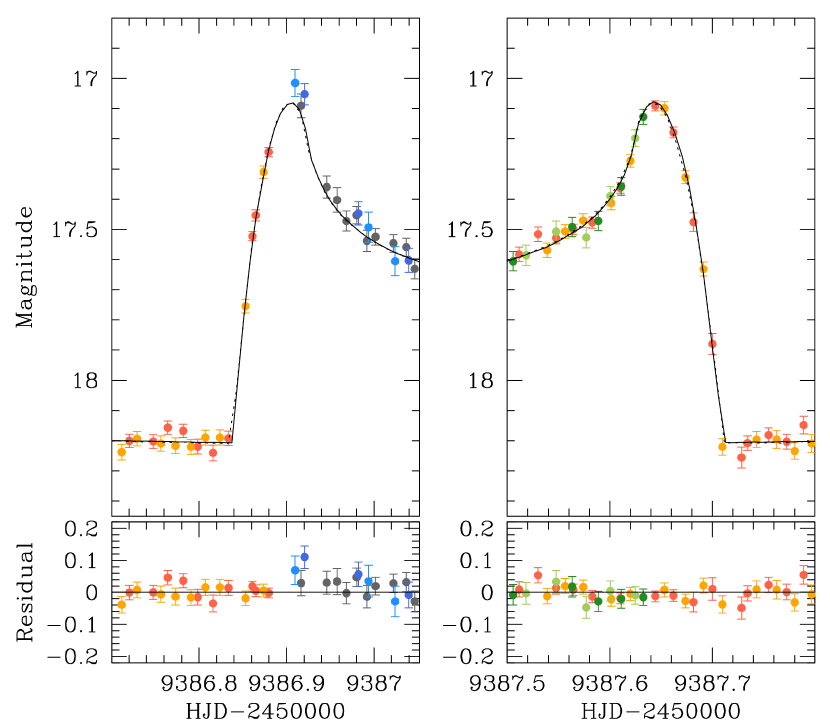
Figure 4: Zoom-in views around the caustic entrance (left panel) and exit (right panel). The solid curve is the model curve of the outer 2L1S solution.

We list the full lensing parameters of the inner and outer 2L1S solutions in Table 1 together with the $\chi^{2}$ values of the fits and degrees of freedom. The two degenerate solutions result in similar mass ratios of $q\sim 1.1\times 10^{-3}$, and the low value of $q$ indicates that the companion to the lens is a planetary mass object. The planet separations of the inner and outer solutions are slightly different from each other, and the separation of the inner solution $s_{\rm in}=1.297\pm 0.005$ is slightly larger than the separation of the outer solution of $s_{\rm out}=1.242\pm 0.007$. Besides these two solutions, we found no other degenerate solutions. For a double check, we investigated a degenerate solution resulting from the off-axis channel by restricting the source trajectory to pass the off-axis cusps, and found that the best-fit off-axis solution resulted in a model that yielded a poorer fit than the outer solution by $\Delta\chi^{2}=2320$.

In Figure 3, we present the model curves of the inner (dotted curve) and outer (solid curve) solutions around the region of the anomaly. It shows that both models well describe the anomaly including the positive deviations caused by caustic crossings and the negative deviations before the caustic entrance and after the caustic exit. As shown in the zoom-in views around the caustic entrance and exit presented in Figure 4, both caustic crossings were densely resolved despite the short duration of each caustic crossing of $\Delta t_{\rm c}\sim 2\rho t_{\rm E}/\sin\psi\sim 2$ hr, where $\psi\sim 70^{\circ}$ represents the incidence angle of the source to the fold of the caustic. With the well resolved caustic crossings, the normalized source radius was precisely measured.

The lens-system configurations of the inner and outer 2L1S solutions are presented in Figure 5, which shows the trajectory of the source with respect to the lens caustic. It shows that the anomaly was produced by the crossings of the source over the planetary caustic formed by a planetary companion, and the source crossed the near and far side according to the inner and outer solutions, respectively. The source crossed the planet-host axis at a very nearly right angle, 89.4 deg, and this explains the near-peak location of the anomaly. The lens-source separation (scaled to $\theta_{\rm E}$) at the time of the anomaly, $u_{\rm anom}\sim 0.5$, is not small, and this explains the low lensing magnification at the time of the anomaly.

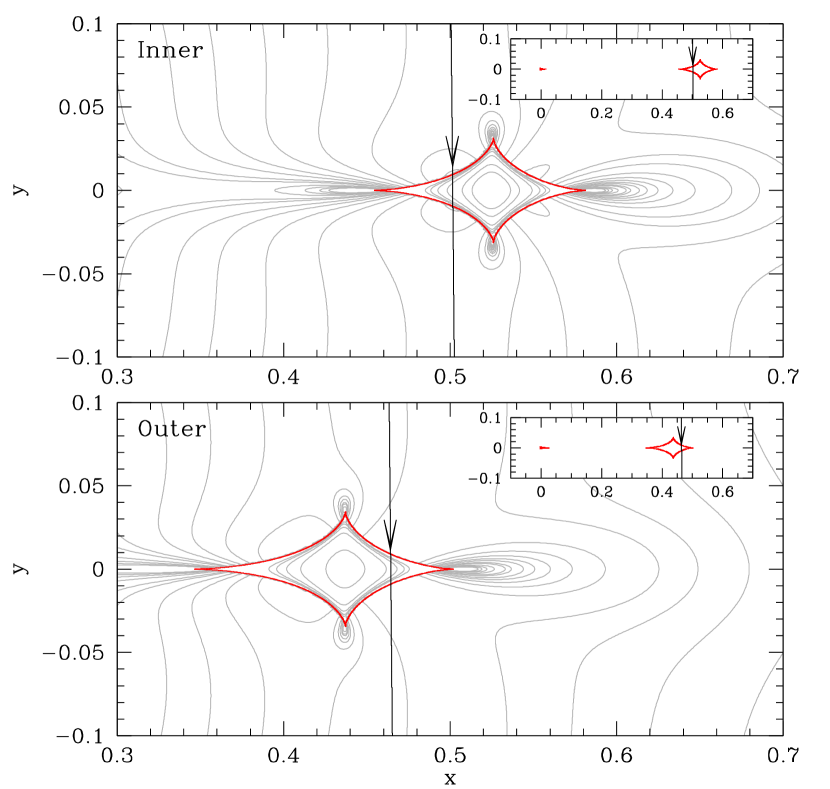
Figure 5: Lens-system configurations of the inner (upper panel) and outer (lower panel) solutions. The inset in each panel shows the whole view of the caustic (red figures), and the main panel shows the zoom-in view around the planetary caustic. The arrowed line represents the source trajectory, and the grey curves encompassing the caustic are equi-magnification contours.

We found that the pair of the planet separations of the inner and outer solutions, $(s_{\rm in},s_{\rm out})$, well obeyed the analytic relation introduced by Hwang et al. (2022). The relation is expressed as

$$s^{\dagger}=\sqrt{s_{\rm in}\times s_{\rm out}}={\sqrt{u_{\rm anom}^{2}+4}+u_{\rm anom}\over 2},$$ (1)

where $u^{2}_{\rm anom}=\tau^{2}_{\rm anom}+u_{0}^{2}$, $\tau_{\rm anom}=(t_{\rm anom}-t_{0})/t_{\rm E}$, and $t_{\rm anom}$ represents the time of the anomaly. We note that the second term in Equation (1) was originally expressed as the arithmetic mean of $s_{\rm in}$ and $s_{\rm out}$, that is, $(s_{\rm in}+s_{\rm out})/2$, and Gould et al. (2022) found that the geometric mean, this is, $(s_{\rm out}\times s_{\rm in})^{1/2}$, proved to be a better approximation than the arithmetic mean. The $s^{\dagger}$ value estimated from $s_{\rm in}$ and $s_{\rm out}$ is $s^{\dagger}=(s_{\rm out}\times s_{\rm in})^{1/2}=1.269$. From the lensing parameters $(t_{0},t_{\rm anom},t_{\rm E})\sim(9387.1,9387.3,43.5)$, it is estimated that $\tau_{\rm anom}=(t_{\rm anom}-t_{0})/t_{\rm E}=0.005$, $u_{\rm anom}=(\tau_{\rm anom}^{2}+u_{0}^{2})^{1/2}=0.480$, and $s^{\dagger}=[(u_{\rm anom}^{2}+4)^{1/2}+u_{\rm anom}]/2=1.269$. Therefore, the $s^{\dagger}$ values estimated from the planet separations $(s_{\rm in},s_{\rm out})$ and from the planetary parameters $(t_{0},t_{\rm anom},u_{0},t_{\rm E})$ match very well down to 3 digits after the decimal point, proving the validity of the analytic relation. In Figure 2, we mark the geometric mean of $s_{\rm in}$ and $s_{\rm out}$ as a dashed vertical line.

We checked whether the microlens parallax $\mbox{\boldmath$\pi$}_{\rm E}$ could be measured by conducting an additional modeling including the two microlens-parallax parameters $(\pi_{{\rm E},N},\pi_{{\rm E},E})$, which denote the north and east components of the microlens-parallax vector $\mbox{\boldmath$\pi$}_{\rm E}=(\mbox{\boldmath$\pi$}_{\rm rel}/\theta_{\rm E})(\mbox{\boldmath$\mu$}/\mu)$, respectively (Gould, 1992, 2000, 2004). Here $\mu$ represents the relative lens-source proper motion vector, $\pi_{\rm rel}=\pi_{\rm L}-\pi_{\rm S}={\rm AU}(1/D_{\rm L}-1/D_{\rm S})$ is the relative lens-source parallax, and $(D_{\rm L},D_{\rm S})$ denote the distances to the lens and source, respectively. We found that it was difficult to measure the parallax parameters because the lensing magnification of the event was low, and thus the light curve was not susceptible to the subtle variation induced by higher-order effects.

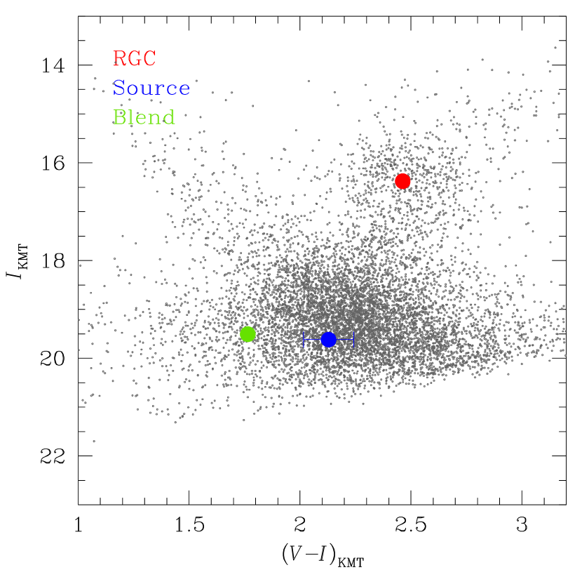
Figure 6: Locations of the source, blend, and red giant clump (RGC) centroid in the instrumental color-magnitude diagram.

4 Source star and Einstein radius

In this section, we characterize the source star of the event and estimate the angular Einstein radius. We estimated $\theta_{\rm E}$ from the relation

$$\theta_{\rm E}={\theta_{*}\over\rho},$$ (2)

where the angular source radius $\theta_{*}$ was deduced from the source type, and the normalized source radius $\rho$ was measured from modeling the light curve. For the specification of the source type, we estimated the reddening- and extinction-corrected (de-reddened) color and magnitude of the source, $(V-I,I)_{{\rm S},0}$.

We used the Yoo et al. (2004) method for the estimation of $(V-I,I)_{{\rm S},0}$. Following the routine procedure of the method, we first measured the instrumental color and magnitude of the source, placed the source in the instrumental color-magnitude diagram (CMD), and then calibrated the source color and magnitude using the centroid of the red giant clump (RGC) in the CMD as a reference. The RGC centroid can serve as a reference for calibration because of its known de-reddened color and magnitude.

In Figure 6, we mark the source position with respect to the RGC centroid in the instrumental CMD constructed using the pyDIA photometry of stars lying around the source. The $I$- and $V$-band magnitudes of the source were measured by regressing the pyDIA photometry data of the individual passbands with respect to the model light curve. The measured colors and magnitudes of the source and RGC centroid are $(V-I,I)_{\rm S}=(2.129\pm 0.113,19.619\pm 0.008)$ and $(V-I,I)_{\rm RGC}=(2.463\pm 0.020,16.377\pm 0.040)$, respectively. We note that the magnitude of the instrumental CMD is approximately scaled, and thus the extinction toward field measured from $I_{\rm RGC}-I_{\rm RGC,0}=1.87$ does not match the value $A_{I}=1.50$ that is estimated from the calibrated magnitude. The measurement uncertainty of $V-I$ is fairly big because the source color was measured mainly on a single $V$-band point inside the caustic trough taken at ${\rm HJD}^{\prime}=9387.584$. With the known de-reddened values of the RGC centroid, $(V-I,I)_{\rm RGC,0}=(1.060,14.502)$ (Bensby et al., 2013; Nataf et al., 2013), then the de-reddened source color and magnitude were estimated as

 

$${(V-I,I)_{\rm 0}=}$$

  (3)

where $\Delta(V-I,I)=(V-I,I)_{\rm S}-(V-I,I)_{\rm RGC}$ represents the offset of the source from the RGC centroid. According to the estimated color and magnitude, the source is a G-type main-sequence star. We note that the error of the dereddened $I$-band magnitude, that is, $\sigma(I_{0})=0.021$ mag, is based purely on the fractional error of the source flux measured from the modeling. Gould (2014) pointed out that the $\theta_{*}$ measurement is subject to additional errors originating from the uncertain dereddened RGC color of Bensby et al. (2013) and the uncertain position of the RGC, and these two errors combined yield a 7% error in the estimation of $\theta_{*}$. In our estimation of $\theta_{*}$, we add this fractional error.

Once the source type was specified, we then estimated the source radius. For the $\theta_{\rm E}$ estimation, we use the Adams et al. (2018) relation of

$$\theta_{*}=0.5\times 10^{[-0.2I_{0}+c_{0}+c_{1}(V-I)_{0}+3]}\leavevmode\nobreak\ \mu{\rm as},$$ (4)

where the values of the coefficients are $c_{0}=0.542\pm 0.007$ and $c_{1}=0.378\pm 0.011$. The measured source radius is

$$\theta_{*}=0.93\pm 0.13\leavevmode\nobreak\ \mu{\rm as},$$ (5)

and this yields the angular Einstein radius

$$\theta_{\rm E}=1.03\pm 0.14\leavevmode\nobreak\ {\rm mas}.$$ (6)

With the measured value of $\theta_{\rm E}$ together with the event time scale $t_{\rm E}$, we estimated the relative lens-source proper motion as

$$\mu={\theta_{\rm E}\over t_{\rm E}}=8.59\pm 1.20\leavevmode\nobreak\ {\rm mas}/{\rm yr}.$$ (7)

Also marked in Figure 6 is the position of the blend (green filled dot), which lies at $(V-I,I)_{\rm b}=(1.76,19.50)$. We checked the possibility that the lens would be the main source of the blended flux by measuring the astrometric offset between the centroid of the source image obtained before the lensing magnification and the centroid of the image obtained at the peak of the lensing magnification. The measured offset is $\delta\theta=(275.95\pm 129.60)$ mas. Considering that the offset is greater than the measurement uncertainty by a factor 2.1, it is unlikely that the main origin of the blended flux is the lens.

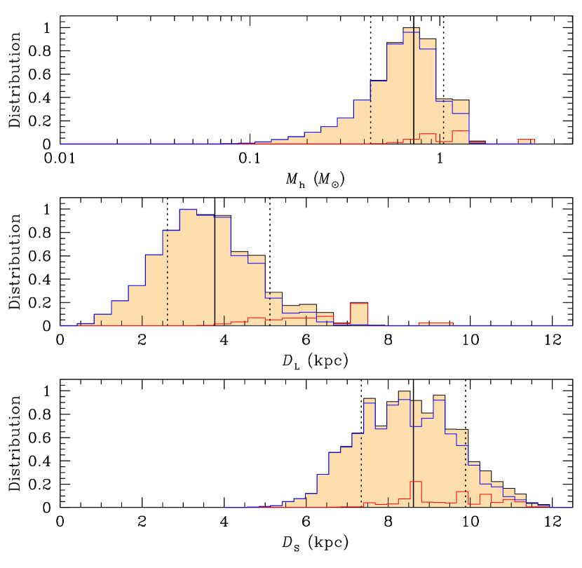
Figure 7: Bayesian posteriors of the primary lens mass and distances to the lens and source. In each panel, the solid vertical line represent the median value, and the two dotted lines represent the 16% and 84% of the distribution.

5 Physical lens parameters

In this section, we estimate the physical parameters of the mass and distance to the lens. For the unique determinations of these parameters, it is required to simultaneously measure the three lensing observables $(t_{\rm E},\theta_{\rm E},\pi_{\rm E})$, from which the parameters are determined by the relations

$$M={\theta_{\rm E}\over\kappa\pi_{\rm E}};\qquad D_{\rm L}={{\rm AU}\over\pi_{\rm E}\theta_{\rm E}+\pi_{\rm S}},$$ (8)

where $\kappa=4G/(c^{2}{\rm AU})\simeq 8.14\leavevmode\nobreak\ {\rm mas}/M_{\odot}$, and $\pi_{\rm S}={\rm AU}/D_{\rm S}$ denotes the parallax of the source (Gould, 2000). For KMT-2021-BLG-1150, the lensing observables $t_{\rm E}$ and $\theta_{\rm E}$ were securely measured, but the other parameter $\pi_{\rm E}$ could not be measured, making it difficult to uniquely determine $M$ and $D_{\rm L}$ using the analytic relations in Equation (8). We, therefore, estimated the physical parameters of the planetary system by conducting a Bayesian analysis based on the measured observables and using a Galactic model. In the analysis, we additionally imposed the lens-brightness constraint given by the fact that the lens cannot be brighter than the blend. It turned out that this constraint had little effect on the Bayesian posteriors.

Table 2: Physical lens parameters

Parameter	Value
$M_{\rm h}$ ($M_{\odot}$)	$0.73^{+0.32}_{-0.30}$
$M_{\rm p}$ ($M_{\rm J}$)	$0.88^{+0.38}_{-0.36}$
$D_{\rm L}$ (kpc)	$3.8^{+1.3}_{-1.2}$
$a_{\perp}$ (AU)	$4.5^{+1.6}_{-1.4}$

Table 3: Variation of planet parameters depending on data

Cadence	Inner		Outer
	$s$	$q$ ($10^{-3}$)	$s$	$q$ ($10^{-3}$)
0.25 hr	$1.297\pm 0.005$	$1.10\pm 0.05$	$1.242\pm 0.007$	$1.15\pm 0.05$
1.0 hr	$1.280\pm 0.008$	$1.29\pm 0.08$	$1.227\pm 0.010$	$1.26\pm 0.06$
2.5 hr	$1.297\pm 0.009$	$1.30\pm 0.09$	$1.273\pm 0.017$	$1.00\pm 0.15$
5.0 hr	$1.297\pm 0.013$	$1.35\pm 0.12$	$1.278\pm 0.024$	$1.08\pm 0.18$

In the Bayesian analysis, we started by generating a large number ($2\times 10^{6}$) of artificial lensing events from the Monte Carlo simulation conducted using a Galactic model and a mass function model of lens objects. The Galactic model defines the physical and dynamical distributions of Galactic objects. In the simulation, we adopted the Galactic and mass function models described in Jung et al. (2021). For each simulated event with $(M_{i},D_{{\rm L},i},\mu_{i})$, we computed the lensing observables using the relations $t_{{\rm E},i}=\theta_{{\rm E},i}/\mu_{i}$ and $\theta_{{\rm E},i}=(\kappa M_{i}\pi_{{\rm rel},i})^{1/2}$, where $\pi_{{\rm rel},i}={\rm AU}(1/D_{{\rm L},i}-1/D_{{\rm S},i})$. Based on the simulated events, posterior distributions of $M$ and $D_{\rm L}$ were constructed by imposing a weight $w_{i}=\exp(-\chi^{2}/2)$ to each artificial event. Here the $\chi^{2}$ value is computed by $\chi^{2}=(t_{{\rm E},i}-t_{\rm E})^{2}/\sigma(t_{\rm E})^{2}+(\theta_{{\rm E},i}-\theta_{\rm E})^{2}/\sigma(\theta_{\rm E})^{2}$, where $(t_{\rm E},\theta_{\rm E})$ represent the measured observables and $[\sigma(t_{\rm E}),\sigma(\theta_{\rm E})]$ denote their measurement uncertainties.

Figure 7 shows the Bayesian posteriors of the mass of the planet host and distances to the lens and source. The physical parameters of the planetary system, including the masses of the host ($M_{\rm h}$) and planet ($M_{\rm p}$), distance, and projected physical separation ($a_{\perp}$) between the planet and host, are listed in Table 2. According to the Bayesian estimation, the lens is a planetary system consisting of a giant planet with a mass $M_{\rm p}=0.88^{+0.38}_{-0.36}\leavevmode\nobreak\ M_{\rm J}$ and its host with a mass $M_{\rm h}=0.73^{+0.32}_{-0.30}\leavevmode\nobreak\ M_{\odot}$ lying toward the Galactic center at a distance $D_{\rm L}=3.8^{+1.3}_{-1.2}$ kpc. Here we adopted the median values of the posterior distributions as representative parameters and the uncertainties were estimated as the 16% and 84% of the distributions. The projected separations estimated from the inner and outer solutions are $a_{\perp,{\rm in}}\sim 4.4$ AU and $a_{\perp,{\rm out}}\sim 4.6$ AU, respectively, and this indicates that the planet lies beyond the snow line, $a_{\rm sl}\sim 2.7(M_{\rm h}/M_{\odot}){\rm AU}\sim 2.0$ AU, of the planetary system regardless of the solutions. Although slightly different, the difference between $a_{\perp,{\rm in}}$ and $a_{\perp,{\rm out}}$ is within the uncertainty of each, and thus we present the mean value in Table 2. We found that the probabilities for the lens to be in the disk and bulge are 93% and 7%, respectively, and thus the host of the planetary system is very likely to be a disk star.

6 Discussion

Degeneracies in the interpretation of a planetary signal may be caused due to either the sparse coverage of the signal or data gaps in the signal. Data gaps can arise when observations cannot be done due to bad weather or when there are gaps between the end of the night at one telescope site and the beginning of the night at another site. In this section, we investigate how the observational cadence and data gaps in microlensing data affect the interpretation of planetary signals by conducting analyses based on mock data sets prepared using those of KMT-2021-BLG-1150 to mimic events with sparse and incomplete data coverage.

Figure 8 shows the anomaly regions of 4 data sets, in which the first 3 sets are generated to mimic data obtained with a 1.0 hr, a 2.5 hr, and a 5.0 hr cadence, and the last one was created to mimic a data set that misses the negative deviations that occur just before the caustic entrance and just after the caustic exit. The three tested observational cadences correspond to those of the KMTNet sub-prime fields, and the assumed 0.25 hr cadence of the last data set corresponds to the cadence of the KMTNet prime field. We note that the anomaly feature is still delineated in the 5-hr-cadence data set.

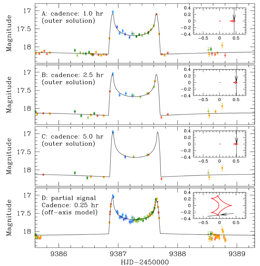
Figure 8: Four sets of mock data. The data sets in the top three panels mimic those obtained with a 1.0 hr, a 2.5 hr, and a 5.0 hr cadence, and the data set in the bottom panel simulate partially covered data. The inset in each panel shows the lens-system configuration of the solution found from modeling, and the solid curve drawn on the data points is the model curve.

In Table 3, we list the planet parameters $(s,q)$ obtained by conducting modeling using the individual mock data sets. It shows that the inner and outer solutions are identified and the variation in the planet parameters among the solutions is not very big, although the measurement uncertainties of the lensing parameters increase as the observational cadence increases. The result of the simulation indicates that the observational cadence does not pose a serious degeneracy problem as long as the anomaly feature is delineated. In the insets of top three panels of Figure  8, we present the lens-system configurations of the outer solutions corresponding to the individual data sets. From the analysis of the partially-covered data set, on the other hand, we were able to identify an off-axis solution, which was decisively rejected in the analysis conducted using the full data set. The planet parameters of the off-axis solution are $(s,q)\sim(0.961\pm 0.001,0.047\pm 0.001)$, which are substantially different from those of the correct solution. The lens system configuration of the off-axis solution is shown in the inset of the bottom panel in Figure 8. Although the fit of the off-axis solution is still substantially worse than the outer solution by $\Delta\chi^{2}\sim 1054$, one finds that the model curve of the off-axis solution appears to approximately describe the caustic features. The identification of the degenerate off-axis solution illustrates that gaps in data can cause degeneracy problems, and this conclusion is further supported by the fact that the recently reported various types of degeneracies were identified from the analyses of partially-covered data sets.

Although the inner and outer solutions are distinct, the effect of the degeneracy on the planet parameters is relatively not severe. This is because the planet parameters of the pair of the inner and outer solutions are similar to each other except for the planetary separation $s$, and even for $s$, the difference between the separations estimated by the two solutions is minor. In the case of KMT-2021-BLG-1150, this difference is $\Delta s=|s_{\rm in}-s_{\rm out}|=0.055$. The difference becomes smaller for lower-mass planets because the size of the planetary caustic decreases as the planet/host mass ratio becomes smaller (Han, 2006). By contrast, the variations in the planet parameters among the lensing solutions resulting from other degeneracy types can be substantial as illustrated by the above off-axis solution and by the recently-reported events with various types of degeneracies found from the analyses of partially covered planetary signals.

We note that the above test has been conducted on an event, that is, KMT-2021-BLG-1150, with a relatively large mass ratio, $q\sim 10^{-3}$. The fact that the event parameters are recovered even when the cadence is greatly reduced supports the original decision of the KMTNet group to survey the majority of the bulge at a 2.5 hour cadence. By contrast, the 10-times higher-cadence observations of the prime fields are designed to capture $q\sim 10^{-5}$ planets, which are 100 times less massive and so have planetary-caustic anomalies that evolve $100^{1/2}=10$ times faster. What is surprising, however, is that even modest gaps in high cadence observations can lead to major degeneracies, even when most of the caustic structure is densely covered.

7 Summary and conclusion

We analyzed the microlensing event KMT-2021-BLG-1150, for which a densely and continuously resolved short-term anomaly appeared in the lensing light curve. From the thorough investigation of the parameter space, we identified a pair of planetary solutions resulting from the well-known inner-outer degeneracy, and found that interpreting the anomaly was not subject to any degeneracy other than the inner-outer degeneracy. The measured planet parameters are $(s,q)_{\rm in}\sim(1.297,1.10\times 10^{-3})$ for the inner solution and $(s,q)_{\rm out}\sim(1.242,1.15\times 10^{-3})$ for the outer solution. We found that the pair of the planet separations of the inner and outer solutions well obeyed the analytic relation introduced by Hwang et al. (2022). According to the physical parameters estimated from a Bayesian analysis, it was found that the lens is a planetary system consisting of a planet with a mass $M_{\rm p}=0.88^{+0.38}_{-0.36}\leavevmode\nobreak\ M_{\rm J}$ and its host with a mass $M_{\rm h}=0.73^{+0.32}_{-0.30}\leavevmode\nobreak\ M_{\odot}$ lying toward the Galactic center at a distance $D_{\rm L}=3.8^{+1.3}_{-1.2}$ kpc. From the analyses conducted using mock data sets prepared to mimic those obtained with data gaps and under various observational cadences, it was found that gaps in data could result in various degenerate solutions, while the observational cadence would not pose a serious degeneracy problem as long as the anomaly feature were be delineated.