Reversible and irreversible bracket-based dynamics for deep graph neural networks

Abstract

Recent works have shown that physics-inspired architectures allow the training of deep graph neural networks (GNNs) without oversmoothing. The role of these physics is unclear, however, with successful examples of both reversible (e.g., Hamiltonian) and irreversible (e.g., diffusion) phenomena producing comparable results despite diametrically opposed mechanisms, and further complications arising due to empirical departures from mathematical theory. This work presents a series of novel GNN architectures based upon structure-preserving bracket-based dynamical systems, which are provably guaranteed to either conserve energy or generate positive dissipation with increasing depth. It is shown that the theoretically principled framework employed here allows for inherently explainable constructions, which contextualize departures from theory in current architectures and better elucidate the roles of reversibility and irreversibility in network performance. Code is available at the Github repository https://github.com/natrask/BracketGraphs.

1 Introduction

Graph neural networks (GNNs) have emerged as a powerful learning paradigm able to treat unstructured data and extract “object-relation”/causal relationships while imparting inductive biases which preserve invariances through the underlying graph topology [1, 2, 3, 4]. This framework has proven effective for a wide range of both graph analytics and data-driven physics modeling problems. Despite successes, GNNs have generally struggle to achieve the improved performance with increasing depth typical of other architectures. Well-known pathologies, such as oversmoothing, oversquashing, bottlenecks, and exploding/vanishing gradients yield deep GNNs which are either unstable or lose performance as the number of layers increase [5, 6, 7, 8].

To combat this, a number of works build architectures which mimic physical processes to impart desirable numerical properties. For example, some works claim that posing message passing as either a diffusion process or reversible flow may promote stability or help retain information, respectively. These present opposite ends of a spectrum between irreversible and reversible processes, which either dissipate or retain information. It is unclear, however, what role (ir)reversibility plays [9]. One could argue that dissipation entropically destroys information and could promote oversmoothing, so should be avoided. Alternatively, in dynamical systems theory, dissipation is crucial to realize a low-dimensional attractor, and thus dissipation may play an important role in realizing dimensionality reduction. Moreover, recent work has shown that dissipative phenomena can actually sharpen information as well as smooth it [10], although this is not often noticed in practice since typical empirical tricks (batch norm, etc.) lead to a departure from the governing mathematical theory.

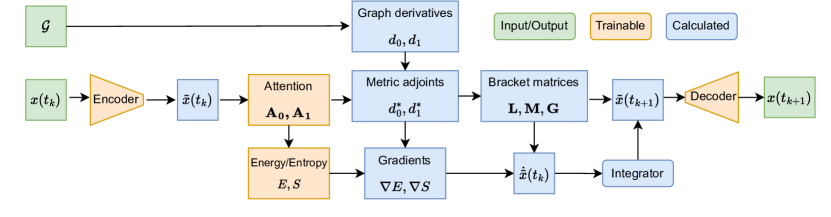
Figure 1: A diagrammatic illustration of the bracket-based architectures introduced in Section 4.

In physics, Poisson brackets and their metriplectic/port-Hamiltonian generalization to dissipative systems provide an abstract framework for studying conservation and entropy production in dynamical systems. In this work, we construct four novel architectures which span the (ir)reversibility spectrum, using geometric brackets as a means of parameterizing dynamics abstractly without empirically assuming a physical model. This relies on an application of the data-driven exterior calculus (DDEC) [11], which allows a reinterpretation of the message-passing and aggregation of graph attention networks [12] as the fluxes and conservation balances of physics simulators [13], providing a simple but powerful framework for mathematical analysis. In this context, we recast graph attention as an inner-product on graph features, inducing graph derivative “building-blocks” which may be used to build geometric brackets. In the process, we generalize classical graph attention [12] to higher-order clique cochains (e.g., labels on edges and loops). The four architectures proposed here scale with identical complexity to classical graph attention networks, and possess desirable properties that have proven elusive in current architectures. On the reversible and irreversible end of the spectrum we have Hamiltonian and Gradient networks. In the middle of the spectrum, Double Bracket and Metriplectic architectures combine both reversibility and irreversibility, dissipating energy to either the environment or an entropic variable, respectively, in a manner consistent with the second law of thermodynamics. We summarize these brackets in Table 1, providing a diagram of their architecture in Figure 1.

Primary contributions:

Theoretical analysis of GAT in terms of exterior calculus. Using DDEC we establish a unified framework for construction and analysis of message-passing graph attention networks, and provide an extensive introductory primer to the theory in the appendices. In this setting, we show that with our modified attention mechanism, GATs amount to a diffusion process for a special choice of activation and weights.

Generalized attention mechanism. Within this framework, we obtain a natural and flexible extension of graph attention from nodal features to higher order cliques (e.g. edge features). We show attention must have a symmetric numerator to be formally structure-preserving, and introduce a novel and flexible graph attention mechanism parameterized in terms of learnable inner products on nodes and edges.

Novel structure-preserving extensions. We develop four GNN architectures based upon bracket-based dynamical systems. In the metriplectic case, we obtain the first architecture with linear complexity in the size of the graph while previous works are $O(N^{3})$.

Unified evaluation of dissipation. We use these architectures to systematically evaluate the role of (ir)reversibility in the performance of deep GNNs. We observe best performance for partially dissipative systems, indicating that a combination of both reversibility and irreversibility are important. Pure diffusion is the least performant across all benchmarks. For physics-based problems including optimal control, there is a distinct improvement. All models provide near state-of-the-art performance and marked improvements over black-box GAT/NODE networks.

Formalism	Equation	Requirements	Completeness	Character
Hamiltonian	$\dot{\mathbf{x}}=\left\{\mathbf{x},E\right\}$	$\mathbf{L}^{*}=-\mathbf{L}$,	complete	conservative
		Jacobi’s identity
Gradient	$\dot{\mathbf{x}}=-\left[\mathbf{x},E\right]$	$\mathbf{M}^{*}=\mathbf{M}$	incomplete	totally dissipative
Double Bracket	$\dot{\mathbf{x}}=\left\{\mathbf{x},E\right\}+\left\{\left\{\mathbf{x},E\right\}\right\}$	$\mathbf{L}^{*}=-\mathbf{L}$	incomplete	partially dissipative
Metriplectic	$\dot{\mathbf{x}}=\left\{\mathbf{x},E\right\}+\left[\mathbf{x},S\right]$	$\mathbf{L}^{*}=-\mathbf{L},\mathbf{M}^{*}=\mathbf{M}$,	complete	partially dissipative
		$\mathbf{L}\nabla S=\mathbf{M}\nabla E=\bm{0}$

Table 1: The abstract bracket formulations employed in this work. Here $\mathbf{x}$ represents a state variable, while $E=E(\mathbf{x}),S=S(\mathbf{x})$ are energy and entropy functions. “Conservative” indicates purely reversible motion, “totally dissipative” indicates purely irreversible motion, and “partially dissipative” indicates motion which either dissipates $E$ (in the double bracket case) or generates $S$ (in the metriplectic case).

2 Previous works

Neural ODEs: Many works use neural networks to fit dynamics of the form $\dot{x}=f(x,\theta)$ to time series data. Model calibration (e.g., UDE [14]), dictionary-based learning (e.g., SINDy [15]), and neural ordinary differential equations (e.g., NODE [16]) pose a spectrum of inductive biases requiring progressively less domain expertise. Structure-preservation provides a means of obtaining stable training without requiring domain knowledge, ideally achieving the flexibility of NODE with the robustness of UDE/SINDy. The current work learns dynamics on a graph while using a modern NODE library to exploit the improved accuracy of high-order integrators [17, 18, 19].

Structure-preserving dense networks: For dense networks, it is relatively straightforward to parameterize reversible dynamics, see for example: Hamiltonian neural networks [20, 21, 22, 23], Hamiltonian generative networks [24], Hamiltonian with Control (SymODEN) [25], Deep Lagrangian networks [26] and Lagrangian neural networks [27]. Structure-preserving extensions to dissipative systems are more challenging, particularly for metriplectic dynamics [28] which require a delicate degeneracy condition to preserve discrete notions of the first and second laws of thermodynamics. For dense networks such constructions are intensive, suffering from $O(N^{3})$ complexity in the number of features [29, 30, 31]. In the graph setting we avoid this and achieve linear complexity by exploiting exact sequence structure. Alternative dissipative frameworks include Dissipative SymODEN [32] and port-Hamiltonian [33]. We choose to focus on metriplectic parameterizations due to their broad potential impact in data-driven physics modeling, and ability to naturally treat fluctuations in multiscale systems [34].

Physics-informed vs structure-preserving: "Physics-informed" learning imposes physics by penalty, adding a regularizer corresponding to a physics residual. The technique is simple to implement and has been successfully applied to solve a range of PDEs [35], discover data-driven models to complement first-principles simulators [36, 37, 38], learn metriplectic dynamics [39], and perform uncertainty quantification [40, 41]. Penalization poses a multiobjective optimization problem, however, with parameters weighting competing objectives inducing pathologies during training, often resulting in physics being imposed to a coarse tolerance and qualitatively poor predictions [42, 43]. In contrast, structure-preserving architectures exactly impose physics by construction via carefully designed networks. Several works have shown that penalty-based approaches suffer in comparison, with structure-preservation providing improved long term stability, extrapolation and physical realizability.

Structure-preserving graph networks: Several works use discretizations of specific PDEs to combat oversmoothing or exploding/vanishing gradients, e.g. telegraph equations [44] or various reaction-diffusion systems [45]. Several works develop Hamiltonian flows on graphs [46, 47]. For metriplectic dynamics, [48] poses a penalty based formulation on graphs. We particularly focus on GRAND, which poses graph learning as a diffusive process [49], using a similar exterior calculus framework and interpreting attention as a diffusion coefficient. We show in Appendix LABEL:app:gats that their analysis fails to account for the asymmetry in the attention mechanism, leading to a departure from the governing theory. To account for this, we introduce a modified attention mechanism which retains interpretation as a part of diffusion PDE. In this purely irreversible case, it is of interest whether adherence to the theory provides improved results, or GRAND’s success is driven by something other than structure-preservation.

3 Theory and fundamentals

Here we introduce the two essential ingredients to our approach: bracket-based dynamical systems for neural differential equations, and the data-driven exterior calculus which enables their construction. A thorough introduction to this material is provided in Appendices LABEL:app:graphcalc, LABEL:app:adjgrad, and LABEL:app:variational.

Bracket-based dynamics: Originally introduced as an extension of Hamiltonian/Lagrangian dynamics to include dissipation [50], bracket formulations are used to inform a dynamical system with certain structural properties, e.g., time-reversibility, invariant differential forms, or property preservation. Even without dissipation, bracket formulations may compactly describe dynamics while preserving core mathematical properties, making them ideal for designing neural architectures.

Bracket formulations are usually specified via some combination of reversible brackets $\left\{F,G\right\}=\left\langle\nabla F,\mathbf{L}\nabla G\right\rangle$ and irreversible brackets $\left[F,G\right]=\left\langle\nabla F,\mathbf{M}\nabla G\right\rangle,\left\{\left\{F,G\right\}\right\}=\left\langle\nabla F,\mathbf{L}^{2}\nabla G\right\rangle$ for potentially state-dependent operators $\mathbf{L}^{*}=-\mathbf{L}$ and $\mathbf{M}^{*}=\mathbf{M}$. The particular brackets which are used in the present network architectures are summarized in Table 1. Note that complete systems are the dynamical extensions of isolated thermodynamical systems: they conserve energy and produce entropy, with nothing lost to the ambient environment. Conversely, incomplete systems do not account for any lost energy: they only require that it vanish in a prescribed way. The choice of completeness is an application-dependent modeling assumption.

Exterior calculus: In the combinatorial Hodge theory [51], an oriented graph $\mathcal{G}=\{\mathcal{V},\mathcal{E}\}$ carries sets of $k$-cliques, denoted $\mathcal{G}_{k}$, which are collections of ordered subgraphs generated by $(k+1)$ nodes. This induces natural exterior derivative operators $d_{k}:\Omega_{k}\to\Omega_{k+1}$, acting on the spaces of functions on $\mathcal{G}_{k}$, which are the signed incidence matrices between $k$-cliques and $(k+1)$-cliques. An explicit representation of these derivatives is given in Appendix LABEL:app:graphcalc, from which it is easy to check the exact sequence property $d_{k+1}\circ d_{k}=0$ for any $k$. This yields a discrete de Rham complex on the graph $\mathcal{G}$ (Figure 2). Moreover, given a choice of inner product (say, $\ell^{2}$) on $\Omega_{k}$, there is an obvious dual de Rham complex which comes directly from adjointness. In particular, one can define dual derivatives $d_{k}^{*}:\Omega_{k+1}\to\Omega_{k}$ via the equality

$$\left\langle d_{k}f,g\right\rangle_{k+1}=\left\langle f,d_{k}^{*}g\right\rangle_{k},$$

from which nontrivial results such as the Hodge decomposition, Poincaré inequality, and coercivity/invertibility of the Hodge Laplacian $\Delta_{k}=d_{k}^{*}d_{k}+d_{k-1}d_{k-1}^{*}$ follow (see e.g. [11]). Using the derivatives $d_{k},d_{k}^{*}$, it is possible to build compatible discretizations of PDEs on $\mathcal{G}$ which are guaranteed to preserve exactness properties such as, e.g., $d_{1}\circ d_{0}=\mathrm{curl}\circ\mathrm{grad}=0$.

The choice of inner product $\left\langle\cdot,\cdot\right\rangle_{k}$ thus induces a definition of the dual derivatives $d_{k}^{*}$. In the graph setting [52], one typically selects the $\ell^{2}$ inner product, obtaining the adjoints of the signed incidence matrices as $d_{k}^{*}=d_{k}^{\intercal}$. By instead working with the modified inner product $\left(\mathbf{v},\mathbf{w}\right)=\mathbf{v}^{\intercal}\mathbf{A}_{k}\mathbf{w}$ for a machine-learnable $\mathbf{A}_{k}$, we obtain $d_{k}^{*}=\mathbf{A}_{k}^{-1}d_{k}^{\intercal}\mathbf{A}_{k+1}$ (see Appendix LABEL:app:adjgrad). This parameterization inherits the exact sequence property from the graph topology encoded in $d_{k}$ while allowing for incorporation of geometric information from data. This leads directly to the following result, which holds for any (potentially feature-dependent) symmetric positive definite matrix $\mathbf{A}_{k}$.

Theorem 3.1.

The dual derivatives $d_{k}^{*}:\Omega_{k+1}\to\Omega_{k}$ adjoint to $d_{k}:\Omega_{k}\to\Omega_{k+1}$ with respect to the learnable inner products $\mathbf{A}_{k}:\Omega_{k}\to\Omega_{k}$ satisfy an exact sequence property.

Proof.

$d_{k-1}^{*}d_{k}^{*}=\mathbf{A}_{k-1}^{-1}d_{k-1}^{\intercal}\mathbf{A}_{k}\mathbf{A}_{k}^{-1}d_{k}^{\intercal}\mathbf{A}_{k+1}=\mathbf{A}_{k-1}^{-1}\left(d_{k}d_{k-1}\right)^{\intercal}\mathbf{A}_{k+1}=0.\qed$

As will be shown in Section 4, by encoding graph attention into the $\mathbf{A}_{k}$, we may exploit the exact sequence property to obtain symmetric positive definite diffusion operators, as well as conduct the cancellations necessary to enforce degeneracy conditions necessary for metriplectic dynamics.

For a thorough review of DDEC, we direct readers to Appendix LABEL:app:graphcalc and [11]. For exterior calculus in topological data analysis see [52], and an overview in the context of PDEs see [53, 54].

Figure 2: A commutative diagram illustrating the relationship between the graph derivatives $d_{k}$, their $\ell^{2}$ adjoints $d_{k}^{\intercal}$, and the learnable adjoints $d_{k}^{*}$. These operators form a de Rham complex due to the exact sequence property $d_{i+1}\circ d_{i}=d^{\intercal}_{i}\circ d^{\intercal}_{i+1}=d^{*}_{i}\circ d^{*}_{i+1}=0$. We show that the learnable $\mathbf{A}_{k}$ may encode attention mechanisms, without impacting the preservation of exact sequence structure.

4 Structure-preserving bracket parameterizations

We next summarize properties of the bracket dynamics introduced in Section 3 and displayed in Table 1, postponing details and rigorous discussion to Appendices LABEL:app:adjgrad and LABEL:app:brackets. Letting $\mathbf{x}=(\mathbf{q},\mathbf{p})$ denote node-edge feature pairs, the following operators will be used to generate our brackets.

$$\mathbf{L}=\begin{pmatrix}0&-d_{0}^{*}\\ d_{0}&0\end{pmatrix},\quad\mathbf{G}=\begin{pmatrix}\Delta_{0}&0\\ 0&\Delta_{1}\end{pmatrix}=\begin{pmatrix}d_{0}^{*}d_{0}&0\\ 0&d_{1}^{*}d_{1}+d_{0}d_{0}^{*}\end{pmatrix},\quad\mathbf{M}=\begin{pmatrix}0&0\\ 0&\mathbf{A}_{1}d_{1}^{*}d_{1}\mathbf{A}_{1}\end{pmatrix}.$$

As mentioned before, the inner products $\mathbf{A}_{0},\mathbf{A}_{1},\mathbf{A}_{2}$ on $\Omega_{k}$ which induce the dual derivatives $d_{0}^{*},d_{1}^{*}$, are chosen in such a way that their combination generalizes a graph attention mechanism. The precise details of this construction are given below, and its relationship to the standard GAT network from [12] is shown in Appendix LABEL:app:gats. Notice that $\mathbf{L}^{*}=-\mathbf{L}$, while $\mathbf{G}^{*}=\mathbf{G},\mathbf{M}^{*}=\mathbf{M}$ are positive semi-definite with respect to the block-diagonal inner product $\left(\cdot,\cdot\right){}$ defined by $\mathbf{A}=\mathrm{diag}\left(\mathbf{A}_{0},\mathbf{A}_{1}\right)$ (details are provided in Appendix LABEL:app:brackets). Therefore, $\mathbf{L}$ generates purely reversible (Hamiltonian) dynamics and $\mathbf{G},\mathbf{M}$ generate irreversible (dissipative) ones. Additionally, note that state-dependence in $\mathbf{L},\mathbf{M},\mathbf{G}$ enters only through the adjoint differential operators, meaning that any structural properties induced by the topology of the graph $\mathcal{G}$ (such as the exact sequence property mentioned in Theorem 3.1) are automatically preserved.

Remark 4.1.

Strictly speaking, $\mathbf{L}$ is guaranteed to be a truly Hamiltonian system only when $d_{0}^{*}$ is state-independent, since it may otherwise fail to satisfy Jacobi’s identity. On the other hand, energy conservation is always guaranteed due to the fact that $\mathbf{L}$ is skew-adjoint.

In addition to the bracket matrices $\mathbf{L},\mathbf{M},\mathbf{G}$, it is necessary to have access to energy and entropy functions $E,S$ and their associated functional derivatives with respect to the inner product on $\Omega_{0}\oplus\Omega_{1}$ defined by $\mathbf{A}$. For the Hamiltonian, gradient, and double brackets, $E$ is chosen simply as the “total kinetic energy”

$$E(\mathbf{q},\mathbf{p})=\frac{1}{2}\left(\left|\mathbf{q}\right|^{2}+\left|\mathbf{p}\right|^{2}\right)=\frac{1}{2}\sum_{i\in\mathcal{V}}\left|\mathbf{q}_{i}\right|^{2}+\frac{1}{2}\sum_{\alpha\in\mathcal{E}}\left|\mathbf{p}_{\alpha}\right|^{2},$$

whose $\mathbf{A}$-gradient (computed in Appendix LABEL:app:brackets) is just $\nabla E(\mathbf{q},\mathbf{p})=\begin{pmatrix}\mathbf{A}_{0}^{-1}\mathbf{q}&\mathbf{A}_{1}^{-1}\mathbf{p}\end{pmatrix}^{\intercal}$. Since the metriplectic bracket uses parameterizations of $E,S$ which are more involved, discussion of this case is deferred to later in this Section.

Attention as learnable inner product: Before describing the dynamics, it remains to discuss how the matrices $\mathbf{A}_{i}$, $0\leq i\leq 2$, are computed in practice, and how they relate to the idea of graph attention. Recall that if $n_{V}>0$ denotes the nodal feature dimension, a graph attention mechanism takes the form $a(\mathbf{q}_{i},\mathbf{q}_{j})=f\left(\tilde{a}_{ij}\right)/\sum_{j}f\left(\tilde{a}_{ij}\right)$ for some differentiable pre-attention function $\tilde{a}:n_{V}\times n_{V}\to\mathbb{R}$ (e.g., for scaled dot product [55]) one typically represents $a(\mathbf{q}_{i},\mathbf{q}_{j})$ as a softmax, so that $f=\exp(\mathbf{q})$). This suggests a decomposition $a(\mathbf{q}_{i},\mathbf{q}_{j})=\mathbf{A}_{0}^{-1}\mathbf{A}_{1}$ where $\mathbf{A}_{0}=\left(a_{0,ii}\right)$ is diagonal on nodes and $\mathbf{A}_{1}=\left(a_{1,ij}\right)$ is diagonal on edges,

$$a_{0,ii}=\sum_{j\in\mathcal{N}(i)}f\left(\tilde{a}\left(\mathbf{q}_{i},\mathbf{q}_{j}\right)\right),\qquad a_{1,ij}=f\left(\tilde{a}\left(\mathbf{q}_{i},\mathbf{q}_{j}\right)\right).$$

Treating the numerator and denominator of the standard attention mechanism separately in $\mathbf{A}_{0},\mathbf{A}_{1}$ allows for a flexible and theoretically sound incorporation of graph attention directly into the adjoint differential operators on $\mathcal{G}$. In particular, if $\mathbf{A}_{1}$ is symmetric with respect to edge-orientation and $\mathbf{p}$ is an edge feature which is antisymmetric, it follows that

$$\left(d_{0}^{*}\mathbf{p}\right)_{i}=\left(\mathbf{A}_{0}^{-1}d_{0}^{\intercal}\mathbf{A}_{1}\mathbf{p}\right)_{i}=\sum_{j\in\mathcal{N}(i)}a\left(\mathbf{q}_{i},\mathbf{q}_{j}\right)\mathbf{p}_{ji},$$

which is just graph attention combined with edge aggregation. This makes it possible to give the following informal statement regarding graph attention networks which is explained and proven in Appendix LABEL:app:gats.

Remark 4.2.

The GAT layer from [12] is almost the forward Euler discretization of a metric heat equation.

The “almost” appearing here has to do with the fact that (1) the attentional numerator $f\left(\tilde{a}(\mathbf{q}_{i},\mathbf{q}_{j})\right)$ is generally asymmetric in $i,j$, and is therefore symmetrized by the divergence operator $d_{0}^{\intercal}$, (2) the activation function between layers is not included, and (3) learnable weight matrices $\mathbf{W}^{k}$ in GAT are set to the identity.

Remark 4.3.

The interpretation of graph attention as a combination of learnable inner products admits a direct generalization to higher-order cliques, which is discussed in Appendix LABEL:app:high-order-attn.

Hamiltonian case: A purely conservative system is generated by solving $\dot{\mathbf{x}}=\mathbf{L}(\mathbf{x})\nabla E(\mathbf{x})$, or

$$\begin{pmatrix}\dot{\mathbf{q}}\\ \dot{\mathbf{p}}\end{pmatrix}=\begin{pmatrix}0&-d_{0}^{*}\\ d_{0}&0\end{pmatrix}\begin{pmatrix}\mathbf{A}_{0}^{-1}&0\\ 0&\mathbf{A}_{1}^{-1}\end{pmatrix}\begin{pmatrix}\mathbf{q}\\ \mathbf{p}\end{pmatrix}=\begin{pmatrix}-d_{0}^{*}\mathbf{A}_{1}^{-1}\mathbf{p}\\ d_{0}\mathbf{A}_{0}^{-1}\mathbf{q}\end{pmatrix}.$$

This is a noncanonical Hamiltonian system which generates a purely reversible flow. In particular, it can be shown that

$$\dot{E}(\mathbf{x})=\left(\dot{\mathbf{x}},\nabla E(\mathbf{x})\right){}=\left(\mathbf{L}(\mathbf{x})\nabla E(\mathbf{x}),\nabla E(\mathbf{x})\right){}=-\left(\nabla E(\mathbf{x}),\mathbf{L}(\mathbf{x})\nabla E(\mathbf{x})\right){}=0,$$

so that energy is conserved due to the skew-adjointness of $\mathbf{L}$.

Gradient case: On the opposite end of the spectrum are generalized gradient flows, which are totally dissipative. Consider solving $\dot{\mathbf{x}}=-\mathbf{G}(\mathbf{x})\nabla E(\mathbf{x})$, or

$$\begin{pmatrix}\dot{\mathbf{q}}\\ \dot{\mathbf{p}}\end{pmatrix}=-\begin{pmatrix}\Delta_{0}&0\\ 0&\Delta_{1}\end{pmatrix}\begin{pmatrix}\mathbf{A}_{0}^{-1}&0\\ 0&\mathbf{A}_{1}^{-1}\end{pmatrix}\begin{pmatrix}\mathbf{q}\\ \mathbf{p}\end{pmatrix}=-\begin{pmatrix}\Delta_{0}\mathbf{A}_{0}^{-1}\mathbf{q}\\ \Delta_{1}\mathbf{A}_{1}^{-1}\mathbf{p}\end{pmatrix}.$$

This system is a metric diffusion process on nodes and edges separately. Moreover, it corresponds to a generalized gradient flow, since

$$\dot{E}(\mathbf{x})=\left(\dot{\mathbf{x}},\nabla E(\mathbf{x})\right){}=-\left(\mathbf{G}(\mathbf{x})\nabla E(\mathbf{x}),\nabla E(\mathbf{x})\right){}=-\left|\nabla E(\mathbf{x})\right|_{\mathbf{G}}^{2}\leq 0,$$

due to the self-adjoint and positive semi-definite nature of $\mathbf{G}$.

Remark 4.4.

The architecture in GRAND [49] is almost a gradient flow, however the pre-attention mechanism lacks the requisite symmetry to formally induce a valid inner product.

Double bracket case: Another useful formulation for incomplete systems is the so-called double-bracket formalism. Consider solving $\dot{\mathbf{x}}=\mathbf{L}\nabla E+\mathbf{L}^{2}\nabla E$, or

$$\begin{pmatrix}\dot{\mathbf{q}}\\ \dot{\mathbf{p}}\end{pmatrix}=\begin{pmatrix}0&-d_{0}^{*}\\ d_{0}&0\end{pmatrix}\begin{pmatrix}\mathbf{A}_{0}^{-1}\mathbf{q}\\ \mathbf{A}_{1}^{-1}\mathbf{p}\end{pmatrix}+\begin{pmatrix}-d_{0}^{*}d_{0}&0\\ 0&-d_{0}d_{0}^{*}\end{pmatrix}\begin{pmatrix}\mathbf{A}_{0}^{-1}\mathbf{q}\\ \mathbf{A}_{1}^{-1}\mathbf{p}\end{pmatrix}=\begin{pmatrix}-\Delta_{0}\mathbf{A}_{0}^{-1}\mathbf{q}-d_{0}^{*}\mathbf{A}_{1}^{-1}\mathbf{p}\\ d_{0}\mathbf{A}_{0}^{-1}\mathbf{q}-d_{0}d_{0}^{*}\mathbf{A}_{1}^{-1}\mathbf{p}\end{pmatrix}.$$

This provides a dissipative relationship which preserves the Casimirs of the Poisson bracket generated by $\mathbf{L}$, since $\mathbf{L}\nabla C=\bm{0}$ implies $\mathbf{L}^{2}\nabla C=\bm{0}$. In particular, it follows that

$$\dot{E}(\mathbf{x})=\left(\dot{\mathbf{x}},\nabla E(\mathbf{x})\right){}=\left(\mathbf{L}(\mathbf{x})\nabla{E}(\mathbf{x})+\mathbf{L}^{2}(\mathbf{x})\nabla E(\mathbf{x}),\nabla E(\mathbf{x})\right){}=0-\left|\mathbf{L}(\mathbf{x})\nabla E(\mathbf{x})\right|^{2}\leq 0,$$

since $\mathbf{L}$ is skew-adjoint and therefore $\mathbf{L}^{2}$ is self-adjoint.

Remark 4.5.

It is interesting to note that the matrix $\mathbf{L}$ is essentially a Dirac operator (square root of the Hodge Laplacian $\Delta=(d+d^{*})^{2}$) restricted to cliques of degree at most 1. However, here $\mathbf{L}^{2}=-\Delta$, so that $\mathbf{L}$ is in some sense “pure imaginary”.

Metriplectic case: Metriplectic systems are expressible as $\dot{\mathbf{x}}=\mathbf{L}\nabla E+\mathbf{M}\nabla S$ where $E,S$ are energy resp. entropy functions which satisfy the degeneracy conditions $\mathbf{L}\nabla S=\mathbf{M}\nabla E=\bm{0}$. One way of setting this up in the present case is to define the energy and entropy functions

$$E(\mathbf{q},\mathbf{p}) =f_{E}\left(s(\mathbf{q})\right)+g_{E}\left(s\left(d_{0}d_{0}^{\intercal}\mathbf{p}\right)\right),$$

$$S(\mathbf{q},\mathbf{p}) =g_{S}\left(s\left(d_{1}^{\intercal}d_{1}\mathbf{p}\right)\right),$$

where $s$ is sum aggregation over nodes resp. edges, $f_{E}:\mathbb{R}^{n_{V}}\to\mathbb{R}$ acts on node features, and $g_{E},g_{S}:\mathbb{R}^{n_{E}}\to\mathbb{R}$ act on edge features. Denoting the “all ones” vector (of variable length) by $\mathbf{1}$, it is shown in Appendix LABEL:app:brackets that the $\mathbf{A}$-gradients of energy and entropy can be computed as

$$\nabla E(\mathbf{x})=\begin{pmatrix}\mathbf{A}_{0}^{-1}\mathbf{1}\otimes\nabla f_{E}\left(h(\mathbf{q})\right)\\ \mathbf{A}_{1}^{-1}d_{0}d_{0}^{\intercal}\mathbf{1}\otimes\nabla g_{E}\left(h\left(d_{0}d_{0}^{\intercal}\mathbf{p}\right)\right)\end{pmatrix},\qquad\nabla S(\mathbf{x})=\begin{pmatrix}0\\ \mathbf{A}_{1}^{-1}d_{1}^{\intercal}d_{1}\mathbf{1}\otimes\nabla g_{S}\left(h\left(d_{1}^{\intercal}d_{1}\mathbf{p}\right)\right)\end{pmatrix}.$$

Similarly, it is shown in Appendix LABEL:app:brackets that the degeneracy conditions $\mathbf{L}\nabla S=\mathbf{M}\nabla E=\bm{0}$ are satisfied by construction. Therefore, the governing dynamical system becomes

$$\begin{pmatrix}\dot{\mathbf{q}}\\ \dot{\mathbf{p}}\end{pmatrix} =\mathbf{L}\nabla E+\mathbf{M}\nabla S=\begin{pmatrix}-\mathbf{A}_{0}^{-1}d_{0}^{\intercal}d_{0}d_{0}^{\intercal}\mathbf{1}\otimes\nabla g_{E}\left(s\left(d_{0}d_{0}^{\intercal}\mathbf{p}\right)\right)\\ d_{0}\mathbf{A}_{0}^{-1}\mathbf{1}\otimes\nabla f_{E}\left(s(\mathbf{q})\right)+\mathbf{A}_{1}d_{1}^{*}d_{1}d_{1}^{\intercal}d_{1}\mathbf{1}\otimes\nabla g_{S}\left(s\left(d_{1}^{\intercal}d_{1}\mathbf{p}\right)\right)\end{pmatrix}.$$

With this, it follows that the system obeys a version of the first and second laws of thermodynamics,

$$\dot{E}(\mathbf{x}) =\left(\dot{\mathbf{x}},\nabla E(\mathbf{x})\right)=\left(\mathbf{L}\nabla E(\mathbf{x}),\nabla E(\mathbf{x})\right)+\left(\mathbf{M}\nabla S(\mathbf{x}),\nabla E(\mathbf{x})\right)=\left(\nabla S(\mathbf{x}),\mathbf{M}\nabla E(\mathbf{x})\right)=0,$$

$$\dot{S}(\mathbf{x}) =\left(\dot{\mathbf{x}},\nabla S(\mathbf{x})\right)=\left(\mathbf{L}\nabla E(\mathbf{x}),\nabla S(\mathbf{x})\right)+\left(\mathbf{M}\nabla S(\mathbf{x}),\nabla S(\mathbf{x})\right)=0+|\nabla S(\mathbf{x})|^{2}_{M}\geq 0.$$

Remark 4.6.

As seen in the increased complexity of this formulation, enforcing the degeneracy conditions necessary for metriplectic structure is nontrivial. This is accomplished presently via an application of the exact sequence property in Theorem 3.1, which we derive in Appendix LABEL:app:brackets.

Remark 4.7.

It is worth mentioning that, similar to the other architectures presented in this Section, the metriplectic network proposed here exhibits linear $O(N)$ scaling in the graph size. This is in notable contrast to [29, 31] which scale as $O(N^{3})$.

5 Experiments

This section reports results on experiments designed to probe the influence of bracket structure on trajectory prediction and nodal feature classification. Additional experimental details can be found in Appendix LABEL:app:exp-details. In each Table, orange indicates the best result by our models, and blue indicates the best of those compared. We consider both physical systems, where the role of structure preservation is explicit, as well as graph-analytic problems.

5.1 Damped double pendulum

As a first experiment, consider applying one of these architectures to reproduce the trajectory of a double pendulum with a damping force proportional to the angular momenta of the pendulum masses (see Appendix LABEL:app:dp-exp-details for details).

Double pendulum	MAE $\mathbf{q}$	MAE $\mathbf{p}$	Total MAE
NODE	$0.0240\pm 0.015$	$0.0299\pm 0.0091$	$0.0269\pm 0.012$
NODE+AE	$0.0532\pm 0.029$	$0.0671\pm 0.043$	$0.0602\pm 0.035$
Hamiltonian	$0.00368\pm 0.0015$	$0.00402\pm 0.0015$	$0.00369\pm 0.0013$
Gradient	$0.00762\pm 0.0023$	$0.0339\pm 0.012$	$0.0208\pm 0.0067$
Double Bracket	$0.00584\pm 0.0013$	$0.0183\pm 0.0071$	$0.0120\pm 0.0037$
Metriplectic	$0.00364\pm 0.00064$	$0.00553\pm 0.00029$	$0.00459\pm 0.00020$

Table 2: Mean absolute errors (MAEs) of the network predictions in the damped double pendulum case, reported as avg$\pm$stdev over 5 runs.

Since this system is metriplectic when expressed in position-momentum-entropy coordinates (c.f. [56]), it is useful to see if any of the brackets from Section 4 can adequately capture these dynamics without an entropic variable. The results of applying the architectures of Section 4 to reproduce a trajectory of five periods are displayed in Table 2, alongside comparisons with a black-box NODE network and a latent NODE with feature encoder/decoder. While each network is capable of producing a small mean absolute error, it is clear that the metriplectic and Hamiltonian networks produce the most accurate trajectories. It is remarkable both that the Hamiltonian bracket does so well here and that the gradient bracket does so poorly, being that the damped double pendulum system is quite dissipative. On the other hand, it is unlikely to be only the feature encoder/decoder leading to good performance here, as both the NODE and NODE+AE architectures perform worse on this task by about one order of magnitude.

5.2 MuJoCo Dynamics

Next we test the proposed models on more complex physical systems that are generated by the Multi-Joint dynamics with Contact (MuJoCo) physics simulator [57]. We consider the modified versions of Open AI Gym environments [23]: HalfCheetah, Hopper, and Swimmer.

We represent an object in an environment as a fully-connected graph, where a node corresponds to a body part of the object and, thus, the nodal feature $\mathbf{q}_{i}$ corresponds to a position of a body part or an angle of a joint. As the edge features, a pair of nodal velocities $\mathbf{p}_{\alpha}=(v_{\text{src}(\alpha)},v_{\text{dst}(\alpha)})$ are provided, where $v_{\text{src}(\alpha)}$ and $v_{\text{dst}(\alpha)}$ denote velocities of the source and destination nodes connected to the edge.

Since the MuJoCo environments contain an actor applying controls, additional control input is accounted for with an additive forcing term which is parameterized by a multi-layer perceptron and introduced into the bracket-based dynamics models. See Appendix LABEL:app:mujoco-exp-details for additional experimental details. The problem therefore consists of finding an optimal control MLP, and we evaluate the improvement which comes from representing the physics surrogate with bracket dynamics over NODE.

All models are trained via minimizing the MSE between the predicted positions $\tilde{\mathbf{q}}$ and the ground truth positions $\mathbf{q}$ and are tested on an unseen test set. Table 3 reports the errors of network predictions on the test set measured in the relative $\ell_{2}$ norm, ${\|{\mathbf{q}}-\tilde{\mathbf{q}}\|_{2}}/{\|\mathbf{q}\|_{2}\|\tilde{\mathbf{q}}\|_{2}}$. Similar to the double pendulum experiments, all models are able to produce accurate predictions with around or less than $10\%$ errors. While the gradient bracket makes little to no improvements over NODEs, the Hamiltonian, double, and metriplectic brackets produce more accurate predictions. Interestingly, the Hamiltonian bracket performs the best in this case as well, meaning that any dissipation present is effectively compensated for by the autoencoder which transforms the features.

Dataset	HalfCheetah	Hopper	Swimmer
NODE+AE	0.106 $\pm$ 0.0011	0.0780 $\pm$ 0.0021	0.0297 $\pm$ 0.0036
Hamiltonian	0.0566 $\pm$ 0.013	0.0279 $\pm$ 0.0019	0.0122 $\pm$ 0.00044
Gradient	0.105 $\pm$ 0.0076	0.0848 $\pm$ 0.0011	0.0290 $\pm$ 0.0011
Double Bracket	0.0621 $\pm$ 0.0096	0.0297 $\pm$ 0.0048	0.0128 $\pm$ 0.00070
Metriplectic	0.105 $\pm$ 0.0091	0.0398 $\pm$ 0.0057	0.0179 $\pm$ 0.00059

Table 3: Relative error of network predictions for the MuJoCo environment on the test set, reported as avg$\pm$stdev over 4 runs.

5.3 Node classification

Moving beyond physics-based examples, it remains to see how bracket-based architectures perform on “black-box” node classification problems. Table 4 and Table 5 present results on common benchmark problems including the citation networks Cora [58], Citeseer [59], and Pubmed [60], as well as the coauthor graph, CoauthorCS [61], and the Amazon co-purchasing graphs, Computer and Photo [62]. For comparison, we report results on a standard GAT [12], a neural graph differential equation architecture (GDE) [63], and the nonlinear GRAND architecture (GRAND-nl) from [49] which is closest to ours. Since our experimental setting is similar to that of [49], the numbers reported for GAT, GDE, and GRAND-nl are taken directly from this paper. Note that, despite the similar $O(N)$ scaling in the metriplectic architecture, the high dimension of the node and edge features on the latter three datasets led to trainable $E,S$ functions which exhausted the memory on our available machines, and therefore results are not reported for these cases. A full description of experimental details is provided in Appendix LABEL:app:node-exp-details.

Remark 5.1.

To highlight the effect of bracket structure on network performance, only minimal modifications are employed during network training. In particular, we do not include any additional regularization, positional encoding, graph rewiring, extraction of connected components, extra terms on the right-hand side, or early stopping. While it is likely that better classification performance could be achieved with some of these modifications included, it becomes very difficult to isolate the effect of structure-preservation. A complete list of tunable hyperparameters is given in Appendix LABEL:app:node-exp-details.

The results show different behavior produced by each bracket architecture. It is empirically clear that there is some value in full or partial reversibility, since the Hamiltonian and double bracket architectures both perform better than the corresponding gradient architecture on datasets such as Computer and Photo. Moreover, it appears that the partially reversible double bracket performs the best of the bracket architectures in every case, which is consistent with the idea that both reversible and irreversible dynamics are critical for capturing the behavior of general dynamical systems. Interestingly, the metriplectic bracket performs worse on these tasks by a large margin. We conjecture this architecture may be harder to train for larger problems despite its $O(N)$ complexity in the graph size, suggesting that more sophisticated training strategies may be required for large problems.

Planetoid splits	CORA	CiteSeer	PubMed
GAT	$82.8\pm 0.5$	$69.5\pm 0.9$	$79.0\pm 0.5$
GDE	$83.8\pm 0.5$	$72.5\pm 0.5$	$79.9\pm 0.3$
GRAND-nl	$83.6\pm 0.5$	$70.8\pm 1.1$	$79.7\pm 0.3$
Hamiltonian	$77.2\pm 0.7$	$73.0\pm 1.2$	$78.5\pm 0.3$
Gradient	$79.9\pm 0.7$	$71.8\pm 1.4$	$78.6\pm 0.7$
Double Bracket	$82.6\pm 0.9$	$74.2\pm 1.4$	$79.6\pm 0.6$
Metriplectic	$57.4\pm 1.0$	$60.5\pm 1.1$	$69.8\pm 0.7$

Table 4: Test accuracy and standard deviations (averaged over 20 randomly initialized runs) using the original Planetoid train-valid-test splits. Comparisons use the numbers reported in [49].

Random splits	CORA	CiteSeer	PubMed	Coauthor CS	Computer	Photo
GAT	$81.8\pm 1.3$	$71.4\pm 1.9$	$78.7\pm 2.3$	$90.5\pm 0.6$	$78.0\pm 19.0$	$85.7\pm 20.3$
GDE	$78.7\pm 2.2$	$71.8\pm 1.1$	$73.9\pm 3.7$	$91.6\pm 0.1$	$82.9\pm 0.6$	$92.4\pm 2.0$
GRAND-nl	$82.3\pm 1.6$	$70.9\pm 1.0$	$77.5\pm 1.8$	$92.4\pm 0.3$	$82.4\pm 2.1$	$92.4\pm 0.8$
Hamiltonian	$76.2\pm 2.1$	$72.2\pm 1.9$	$76.8\pm 1.1$	$92.0\pm 0.2$	$84.0\pm 1.0$	$91.8\pm 0.2$
Gradient	$81.3\pm 1.2$	$72.1\pm 1.7$	$77.2\pm 2.1$	$92.2\pm 0.3$	$78.1\pm 1.2$	$88.2\pm 0.6$
Double Bracket	$83.0\pm 1.1$	$74.2\pm 2.5$	$78.2\pm 2.0$	$92.5\pm 0.2$	$84.8\pm 0.5$	$92.4\pm 0.3$
Metriplectic	$59.6\pm 2.0$	$63.1\pm 2.4$	$69.8\pm 2.1$	-	-	-

Table 5: Test accuracy and standard deviations averaged over 20 runs with random 80/10/10 train/val/test splits. Comparisons use the numbers reported in [49].

6 Conclusion

This work presents a unified theoretical framework for analysis and construction of graph attention networks. The exact sequence property of graph derivatives and coercivity of Hodge Laplacians which follow from the theory allow the construction of four structure-preserving brackets, which we use to evaluate the role of irreversibility in both data-driven physics simulators and graph analytics problems. In all contexts, the pure diffusion bracket performed most poorly, with mixed results between purely reversible and partially dissipative brackets.

The linear scaling achieved by the metriplectic brackets has a potential major impact for data-driven physics modeling. Metriplectic systems emerge naturally when coarse-graining multiscale systems. With increasing interest in using ML to construct digital twins, fast data-driven surrogates for complex multi-physics acting over multiple scales will become crucial. In this setting the stability encoded by metriplectic dynamics translates to robust surrogates, with linear complexity suggesting the possibility of scaling up to millions of degrees of freedom.

Limitations:

All analysis holds under the assumption of modified attention mechanisms which allow interpretation of GAT networks as diffusion processes; readers should take care that the analysis is for a non-standard attention. Secondly, for all brackets we did not introduce empirical modifications (e.g. regularization, forcing, etc) to optimize performance so that we could study the role of (ir)reversibility in isolation. With this in mind, one may be able to add “tricks” to e.g. obtain a diffusion architecture which outperforms those presented here. Finally, note that the use of a feature autoencoder in the bracket architectures means that structure is enforced in the transformed space. This allows for applicability to more general systems, and can be easily removed when appropriate features are known.

Broader impacts:

The work performed here is strictly foundational mathematics and is intended to improve the performance of GNNs in the context of graph analysis and data-driven physics modeling. Subsequent application of the theory may have societal impact, but the current work anticipated to improve the performance of machine learning in graph settings only at a foundational level.

References

- [1] Marco Gori, Gabriele Monfardini, and Franco Scarselli. A new model for learning in graph domains. In Proceedings. 2005 IEEE International Joint Conference on Neural Networks, 2005., volume 2, pages 729–734. IEEE, 2005.
- [2] Jie Zhou, Ganqu Cui, Shengding Hu, Zhengyan Zhang, Cheng Yang, Zhiyuan Liu, Lifeng Wang, Changcheng Li, and Maosong Sun. Graph neural networks: A review of methods and applications. AI open, 1:57–81, 2020.
- [3] Will Hamilton, Zhitao Ying, and Jure Leskovec. Inductive representation learning on large graphs. Advances in neural information processing systems, 30, 2017.
- [4] William L Hamilton, Rex Ying, and Jure Leskovec. Representation learning on graphs: Methods and applications. arXiv preprint arXiv:1709.05584, 2017.
- [5] Deli Chen, Yankai Lin, Wei Li, Peng Li, Jie Zhou, and Xu Sun. Measuring and relieving the over-smoothing problem for graph neural networks from the topological view. In Proceedings of the AAAI conference on artificial intelligence, volume 34, pages 3438–3445, 2020.
- [6] Michael M Bronstein, Joan Bruna, Taco Cohen, and Petar Veličković. Geometric deep learning: Grids, groups, graphs, geodesics, and gauges. arXiv preprint arXiv:2104.13478, 2021.
- [7] Kaixiong Zhou, Xiao Huang, Yuening Li, Daochen Zha, Rui Chen, and Xia Hu. Towards deeper graph neural networks with differentiable group normalization. Advances in neural information processing systems, 33:4917–4928, 2020.
- [8] Chen Cai and Yusu Wang. A note on over-smoothing for graph neural networks. arXiv preprint arXiv:2006.13318, 2020.
- [9] Yifei Wang, Yisen Wang, Jiansheng Yang, and Zhouchen Lin. Dissecting the diffusion process in linear graph convolutional networks. Advances in Neural Information Processing Systems, 34:5758–5769, 2021.
- [10] Francesco Di Giovanni, James Rowbottom, Benjamin P. Chamberlain, Thomas Markovich, and Michael M. Bronstein. Understanding convolution on graphs via energies, 2023.
- [11] Nathaniel Trask, Andy Huang, and Xiaozhe Hu. Enforcing exact physics in scientific machine learning: a data-driven exterior calculus on graphs. arXiv preprint arXiv:2012.11799, 2020.
- [12] Petar Veličković, Guillem Cucurull, Arantxa Casanova, Adriana Romero, Pietro Lio, and Yoshua Bengio. Graph attention networks. arXiv preprint arXiv:1710.10903, 2017.
- [13] Khemraj Shukla, Mengjia Xu, Nathaniel Trask, and George E Karniadakis. Scalable algorithms for physics-informed neural and graph networks. Data-Centric Engineering, 3:e24, 2022.
- [14] Christopher Rackauckas, Yingbo Ma, Julius Martensen, Collin Warner, Kirill Zubov, Rohit Supekar, Dominic Skinner, Ali Ramadhan, and Alan Edelman. Universal differential equations for scientific machine learning. arXiv preprint arXiv:2001.04385, 2020.
- [15] Steven L Brunton, Joshua L Proctor, and J Nathan Kutz. Discovering governing equations from data by sparse identification of nonlinear dynamical systems. Proceedings of the national academy of sciences, 113(15):3932–3937, 2016.
- [16] Ricky TQ Chen, Yulia Rubanova, Jesse Bettencourt, and David Duvenaud. Neural ordinary differential equations. In Proceedings of the 32nd International Conference on Neural Information Processing Systems, pages 6572–6583, 2018.
- [17] Michael Poli, Stefano Massaroli, Atsushi Yamashita, Hajime Asama, Jinkyoo Park, and Stefano Ermon. Torchdyn: Implicit models and neural numerical methods in pytorch. ddd, 2020.
- [18] Louis-Pascal Xhonneux, Meng Qu, and Jian Tang. Continuous graph neural networks. In International Conference on Machine Learning, pages 10432–10441. PMLR, 2020.
- [19] Fangda Gu, Heng Chang, Wenwu Zhu, Somayeh Sojoudi, and Laurent El Ghaoui. Implicit graph neural networks. Advances in Neural Information Processing Systems, 33:11984–11995, 2020.
- [20] Samuel Greydanus, Misko Dzamba, and Jason Yosinski. Hamiltonian neural networks. In H. Wallach, H. Larochelle, A. Beygelzimer, F. d'Alché-Buc, E. Fox, and R. Garnett, editors, Advances in Neural Information Processing Systems, volume 32. Curran Associates, Inc., 2019.
- [21] Marc Finzi, Ke Alexander Wang, and Andrew G Wilson. Simplifying hamiltonian and lagrangian neural networks via explicit constraints. Advances in neural information processing systems, 33:13880–13889, 2020.
- [22] Renyi Chen and Molei Tao. Data-driven prediction of general hamiltonian dynamics via learning exactly-symplectic maps. In International Conference on Machine Learning, pages 1717–1727. PMLR, 2021.
- [23] Nate Gruver, Marc Anton Finzi, Samuel Don Stanton, and Andrew Gordon Wilson. Deconstructing the inductive biases of hamiltonian neural networks. In International Conference on Learning Representations, 2020.
- [24] Peter Toth, Danilo J Rezende, Andrew Jaegle, Sébastien Racanière, Aleksandar Botev, and Irina Higgins. Hamiltonian generative networks. In International Conference on Learning Representations, 2019.
- [25] Yaofeng Desmond Zhong, Biswadip Dey, and Amit Chakraborty. Symplectic ODE-Net: Learning Hamiltonian dynamics with control. In International Conference on Learning Representations, 2019.
- [26] Michael Lutter, Christian Ritter, and Jan Peters. Deep lagrangian networks: Using physics as model prior for deep learning. In International Conference on Learning Representations, 2018.
- [27] Miles Cranmer, Sam Greydanus, Stephan Hoyer, Peter Battaglia, David Spergel, and Shirley Ho. Lagrangian neural networks. In ICLR 2020 Workshop on Integration of Deep Neural Models and Differential Equations, 2020.
- [28] Partha Guha. Metriplectic structure, leibniz dynamics and dissipative systems. Journal of Mathematical Analysis and Applications, 326(1):121–136, 2007.
- [29] Kookjin Lee, Nathaniel Trask, and Panos Stinis. Machine learning structure preserving brackets for forecasting irreversible processes. Advances in Neural Information Processing Systems, 34:5696–5707, 2021.
- [30] Kookjin Lee, Nathaniel Trask, and Panos Stinis. Structure-preserving sparse identification of nonlinear dynamics for data-driven modeling. In Mathematical and Scientific Machine Learning, pages 65–80. PMLR, 2022.
- [31] Zhen Zhang, Yeonjong Shin, and George Em Karniadakis. Gfinns: Generic formalism informed neural networks for deterministic and stochastic dynamical systems. Philosophical Transactions of the Royal Society A, 380(2229):20210207, 2022.
- [32] Yaofeng Desmond Zhong, Biswadip Dey, and Amit Chakraborty. Dissipative symoden: Encoding hamiltonian dynamics with dissipation and control into deep learning. In ICLR 2020 Workshop on Integration of Deep Neural Models and Differential Equations, 2020.
- [33] Shaan A Desai, Marios Mattheakis, David Sondak, Pavlos Protopapas, and Stephen J Roberts. Port-hamiltonian neural networks for learning explicit time-dependent dynamical systems. Physical Review E, 104(3):034312, 2021.
- [34] Miroslav Grmela. Generic guide to the multiscale dynamics and thermodynamics. Journal of Physics Communications, 2(3):032001, 2018.
- [35] Maziar Raissi, Paris Perdikaris, and George E Karniadakis. Physics-informed neural networks: A deep learning framework for solving forward and inverse problems involving nonlinear partial differential equations. Journal of Computational physics, 378:686–707, 2019.
- [36] Maziar Raissi and George Em Karniadakis. Hidden physics models: Machine learning of nonlinear partial differential equations. Journal of Computational Physics, 357:125–141, 2018.
- [37] Filippo Masi and Ioannis Stefanou. Multiscale modeling of inelastic materials with thermodynamics-based artificial neural networks (tann). Computer Methods in Applied Mechanics and Engineering, 398:115190, 2022.
- [38] Ravi G Patel, Indu Manickam, Nathaniel A Trask, Mitchell A Wood, Myoungkyu Lee, Ignacio Tomas, and Eric C Cyr. Thermodynamically consistent physics-informed neural networks for hyperbolic systems. Journal of Computational Physics, 449:110754, 2022.
- [39] Quercus Hernández, Alberto Badías, David González, Francisco Chinesta, and Elías Cueto. Structure-preserving neural networks. Journal of Computational Physics, 426:109950, 2021.
- [40] Yibo Yang and Paris Perdikaris. Adversarial uncertainty quantification in physics-informed neural networks. Journal of Computational Physics, 394:136–152, 2019.
- [41] Dongkun Zhang, Lu Lu, Ling Guo, and George Em Karniadakis. Quantifying total uncertainty in physics-informed neural networks for solving forward and inverse stochastic problems. Journal of Computational Physics, 397:108850, 2019.
- [42] Sifan Wang, Yujun Teng, and Paris Perdikaris. Understanding and mitigating gradient flow pathologies in physics-informed neural networks. SIAM Journal on Scientific Computing, 43(5):A3055–A3081, 2021.
- [43] Sifan Wang, Xinling Yu, and Paris Perdikaris. When and why pinns fail to train: A neural tangent kernel perspective. Journal of Computational Physics, 449:110768, 2022.
- [44] T Konstantin Rusch, Ben Chamberlain, James Rowbottom, Siddhartha Mishra, and Michael Bronstein. Graph-coupled oscillator networks. In International Conference on Machine Learning, pages 18888–18909. PMLR, 2022.
- [45] Jeongwhan Choi, Seoyoung Hong, Noseong Park, and Sung-Bae Cho. Gread: Graph neural reaction-diffusion equations. arXiv preprint arXiv:2211.14208, 2022.
- [46] Alvaro Sanchez-Gonzalez, Victor Bapst, Kyle Cranmer, and Peter Battaglia. Hamiltonian graph networks with ode integrators. arXiv preprint arXiv:1909.12790, 2019.
- [47] Suresh Bishnoi, Ravinder Bhattoo, Jayadeva Jayadeva, Sayan Ranu, and NM Anoop Krishnan. Enhancing the inductive biases of graph neural ode for modeling physical systems. In The Eleventh International Conference on Learning Representations, 2022.
- [48] Quercus Hernandez, Alberto Badias, Francisco Chinesta, and Elias Cueto. Thermodynamics-informed graph neural networks. IEEE Transactions on Artificial Intelligence, 1(01):1–1, 2022.
- [49] Ben Chamberlain, James Rowbottom, Maria I Gorinova, Michael Bronstein, Stefan Webb, and Emanuele Rossi. Grand: Graph neural diffusion. In International Conference on Machine Learning, pages 1407–1418. PMLR, 2021.
- [50] PJ Morrison. Thoughts on brackets and dissipation: old and new. In Journal of Physics: Conference Series, volume 169, page 012006. IOP Publishing, 2009.
- [51] Oliver Knill. The dirac operator of a graph, 2013.
- [52] Xiaoye Jiang, Lek-Heng Lim, Yuan Yao, and Yinyu Ye. Statistical ranking and combinatorial hodge theory. Mathematical Programming, 127(1):203–244, 2011.
- [53] Pavel B Bochev and James M Hyman. Principles of mimetic discretizations of differential operators. In Compatible spatial discretizations, pages 89–119. Springer, 2006.
- [54] Douglas N Arnold. Finite element exterior calculus. SIAM, 2018.
- [55] Ashish Vaswani, Noam Shazeer, Niki Parmar, Jakob Uszkoreit, Llion Jones, Aidan N Gomez, Ł ukasz Kaiser, and Illia Polosukhin. Attention is all you need. In I. Guyon, U. Von Luxburg, S. Bengio, H. Wallach, R. Fergus, S. Vishwanathan, and R. Garnett, editors, Advances in Neural Information Processing Systems, volume 30. Curran Associates, Inc., 2017.
- [56] Ignacio Romero. Thermodynamically consistent time-stepping algorithms for non-linear thermomechanical systems. International Journal for Numerical Methods in Engineering, 79(6):706–732, 2023/05/14 2009.
- [57] Emanuel Todorov, Tom Erez, and Yuval Tassa. Mujoco: A physics engine for model-based control. In 2012 IEEE/RSJ international conference on intelligent robots and systems, pages 5026–5033. IEEE, 2012.
- [58] Andrew Kachites McCallum, Kamal Nigam, Jason Rennie, and Kristie Seymore. Automating the construction of internet portals with machine learning. Information Retrieval, 3:127–163, 2000.
- [59] Prithviraj Sen, Galileo Namata, Mustafa Bilgic, Lise Getoor, Brian Galligher, and Tina Eliassi-Rad. Collective classification in network data. AI magazine, 29(3):93–93, 2008.
- [60] Galileo Namata, Ben London, Lise Getoor, Bert Huang, and U Edu. Query-driven active surveying for collective classification. In 10th international workshop on mining and learning with graphs, volume 8, page 1, 2012.
- [61] Oleksandr Shchur, Maximilian Mumme, Aleksandar Bojchevski, and Stephan Günnemann. Pitfalls of graph neural network evaluation. ArXiv, abs/1811.05868, 2018.
- [62] Julian McAuley, Christopher Targett, Qinfeng Shi, and Anton Van Den Hengel. Image-based recommendations on styles and substitutes. In Proceedings of the 38th international ACM SIGIR conference on research and development in information retrieval, pages 43–52, 2015.
- [63] Michael Poli, Stefano Massaroli, Junyoung Park, Atsushi Yamashita, Hajime Asama, and Jinkyoo Park. Graph neural ordinary differential equations. arXiv preprint arXiv:1911.07532, 2019.
- [64] Xiaoye Jiang, Lek-Heng Lim, Yuan Yao, and Yinyu Ye. Statistical ranking and combinatorial hodge theory. Mathematical Programming, 127(1):203–244, nov 2010.
- [65] Anthony Bloch, P. S. Krishnaprasad, Jerrold E. Marsden, and Tudor S. Ratiu. The euler-poincaré equations and double bracket dissipation. Communications in Mathematical Physics, 175(1):1–42, 1996.
- [66] Darryl D Holm, Jerrold E Marsden, and Tudor S Ratiu. The euler–poincaré equations and semidirect products with applications to continuum theories. Advances in Mathematics, 137(1):1–81, 1998.
- [67] Hans Christian Oettinger. Irreversible dynamics, onsager-casimir symmetry, and an application to turbulence. Physical Review E, 90(4):042121, 2014.
- [68] Anthony Gruber, Max Gunzburger, Lili Ju, and Zhu Wang. Energetically consistent model reduction for metriplectic systems. Computer Methods in Applied Mechanics and Engineering, 404:115709, 2023.
- [69] Robert J. Renka. A simple explanation of the sobolev gradient method. In A Simple Explanation of the Sobolev Gradient Method, 2006.
- [70] Chris Yu, Henrik Schumacher, and Keenan Crane. Repulsive curves. ACM Trans. Graph., 40(2), may 2021.
- [71] Adam Paszke, Sam Gross, Francisco Massa, Adam Lerer, James Bradbury, Gregory Chanan, Trevor Killeen, Zeming Lin, Natalia Gimelshein, Luca Antiga, et al. Pytorch: An imperative style, high-performance deep learning library. Advances in neural information processing systems, 32, 2019.
- [72] Joe Chen. Chaos from simplicity: an introduction to the double pendulum. Technical report, University of Canterbury, 2008.
- [73] Diederik P Kingma and Jimmy Ba. Adam: A method for stochastic optimization. arXiv preprint arXiv:1412.6980, 2014.
- [74] Romeo Ortega, Arjan Van Der Schaft, Bernhard Maschke, and Gerardo Escobar. Interconnection and damping assignment passivity-based control of port-controlled hamiltonian systems. Automatica, 38(4):585–596, 2002.
- [75] Greg Brockman, Vicki Cheung, Ludwig Pettersson, Jonas Schneider, John Schulman, Jie Tang, and Wojciech Zaremba. OpenAI Gym. arXiv preprint arXiv:1606.01540, 2016.
- [76] Lukas Biewald. Experiment tracking with weights and biases, 2020. Software available from wandb.com.