Semantic Segmentation by Semantic Proportions

Abstract

Semantic segmentation is a critical task in computer vision that aims to identify and classify individual pixels in an image, with numerous applications for example autonomous driving and medical image analysis. However, semantic segmentation can be super challenging particularly due to the need for large amounts of annotated data. Annotating images is a time-consuming and costly process, often requiring expert knowledge and significant effort. In this paper, we propose a novel approach for semantic segmentation by eliminating the need of ground-truth segmentation maps. Instead, our approach requires only the rough information of individual semantic class proportions, shortened as semantic proportions. It greatly simplifies the data annotation process and thus will significantly reduce the annotation time and cost, making it more feasible for large-scale applications. Moreover, it opens up new possibilities for semantic segmentation tasks where obtaining the full ground-truth segmentation maps may not be feasible or practical. Extensive experimental results demonstrate that our approach can achieve comparable and sometimes even better performance against the benchmark method that relies on the ground-truth segmentation maps. Utilising semantic proportions suggested in this work offers a promising direction for future research in the field of semantic segmentation.

1 Introduction

Semantic segmentation is widely resorted in a variety of fields such as autonomous driving [25], medical imaging [1, 28], augmented reality [29] and robotics [18]. Impressive improvements have been shown in those areas with the recent development of deep neural networks (DNNs), benefited from the availability of extensive annotated segmentation datasets at a large scale [10, 12]. However, creating such datasets can be very expensive and time-consuming due to the usual need of annotating pixel-wise labels as it takes between 54 and 79 seconds per object [3], and thus requiring a couple of minutes per image with a few objects. Moreover, requiring full supervision is rather impractical in some cases for example medical imaging where expert knowledge is required. Annotating 3D data for semantic segmentation is even more costly and time-consuming due to the additional complexity and dimensionality of the data, which generally requires voxel (i.e., point in 3D space) annotation. Skilled annotators from outsourcing companies that are dedicated to data annotation may be needed for specific requests to ensure annotation accuracy and consistency, adding further to the cost [11].

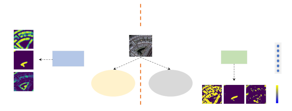
Figure 1: Difference between the proposed semantic segmentation approach and benchmark methods.

Different approaches have been proposed to reduce the fine-grained level (e.g. pixel-wise) annotation costs. One line of research is to train segmentation models in a weakly supervised manner by requiring image-level labels [23, 26], scribbles [15], eye tracks [21] or point supervision [3, 17] rather than costly segmentation masks of individual semantic classes. In contrast, we in this paper propose to utilise the proportion (i.e., percentage information) of each semantic class present in the image for semantic segmentation. For simplicity, we call this type of annotation semantic (class) proportions (SP). To the best of our knowledge, this is the fist time of utilising SP for semantic segmentation. This innovative way, different from the existing ways, could significantly simplify and reduce the human involvement required for data annotation in semantic segmentation. Our proposed semantic segmentation approach by utilising the SP annotation can achieve comparable and sometimes even better performance in comparison to the benchmark method with full supervision utilising the ground-truth segmentation masks, see for example Figure 1.

Our main contributions are: i) propose a new semantic segmentation methodology utilising SP annotations; ii) conduct extensive experiments on representative benchmark datasets from distinct fields to demonstrate the effectiveness and robustness of the proposed approach; iii) draw an insightful discussion for semantic segmentation with weakly annotated data and future directions.

2 Methodology

The semantic segmentation task is to segment an image into different semantic classes/categories.

Notation. Let ${\cal X}$ be a set of images. Without loss of generality, we assume each image in ${\cal X}$ contains no more than $C$ semantic classes. $\forall\boldsymbol{X}_{i}\in{\cal X}$, $\boldsymbol{X}_{i}\in\mathbb{R}^{M\times H}$, where $M\times H$ is the image size. Let ${\cal X}_{\rm T}\subset{\cal X}$ and ${\cal X}_{\rm V}\subset{\cal X}$ be the training and validation (test) sets, respectively. Let ${\Omega}_{\rm T}\subset\mathbb{N}$ be the set containing the indexes of the images in ${\cal X}_{\rm T}$.

$\forall\boldsymbol{X}_{i}\in{\cal X}_{\rm T}$, annotations are available. The most general annotation is the ground-truth segmentation maps, say $\{\boldsymbol{Y}^{*}_{ij}\}_{j=1}^{C}$, for $\boldsymbol{X}_{i}$, where each $\boldsymbol{Y}^{*}_{ij}\in\mathbb{R}^{M\times H}$ is a binary mark for the semantic class $j$ in $\boldsymbol{X}_{i}$. For simplicity, let $\boldsymbol{Y}^{*}_{i}$ be a tensor formed by $\{\boldsymbol{Y}^{*}_{ij}\}_{j=1}^{C}$, where its $j$-th channel is $\boldsymbol{Y}^{*}_{ij}$. Note, importantly, that the ground-truth segmentation maps are not used in our approach for semantic segmentation in this paper unless specifically stated; instead, they are used by the benchmark method for comparison purpose. Analogously, let $\boldsymbol{Y}_{i}$ be the predicted segmentation maps following the same format as $\boldsymbol{Y}^{*}_{i}$. Let $\boldsymbol{\rho}^{*}_{i}=(\rho^{*}_{i1},\cdots,\rho^{*}_{iC})$ be the given SP annotation of image $\boldsymbol{X}_{i}\in{\cal X}_{\rm T}$, which will be used to train our approach, where each $\rho^{*}_{ij}\in[0,1]$ and $\sum_{j=1}^{C}\rho^{*}_{ij}=1$.

Loss function. Two types of loss functions are introduced in the architectures of our method. One is based on the mean squared error (MSE). MSE is commonly used to evaluate the performance of regression models where there are numerical target values to predict. We employ MSE to measure the discrepancy between the ground-truth SP and the predicted ones. For ease of reference, we call this loss function $\mathcal{L}_{\rm sp}$ throughout the paper, i.e.,

$$\mathcal{L}_{\rm sp}=\frac{1}{|{\Omega}_{\rm T}|}\sum_{i\in{\Omega}_{\rm T}}\|\boldsymbol{\rho}^{*}_{i}-\boldsymbol{\rho}_{i}\|^{2},$$ (1)

where $\boldsymbol{\rho}_{i}$ is the predicted SP for image $\boldsymbol{X}_{i}\in{\cal X}_{\rm T}$ and $|{\Omega}_{\rm T}|$ is the cardinality of set ${\Omega}_{\rm T}$.

The other loss function is defined based on the binary cross-entropy (BCE), see Section 2.2 for the detail. BCE is a commonly used loss function in binary classification problems and measures the discrepancy between the predicted probabilities and the true binary ones. Below we define the BCE function for the $j$-th semantic class of image $\boldsymbol{X}_{i}$ at coordinate (location) $(m,h)\in[1,M]\times[1,H]$ as

$$f_{ij}(m,h)=-\left(\boldsymbol{Y}^{*}_{ij}[m,h]\log(\boldsymbol{Y}_{ij}[m,h])+(1-\boldsymbol{Y}^{*}_{ij}[m,h])\log(1-\boldsymbol{Y}_{ij}[m,h])\right),$$ (2)

where $\boldsymbol{Y}_{ij}$ is the predicted segmentation map for the $j$-th semantic class of image $\boldsymbol{X}_{i}$ and $\boldsymbol{Y}_{ij}[m,h]$ is the value of $\boldsymbol{Y}_{ij}$ at coordinate $(m,h)$.

2.1 Proposed SP-based Semantic Segmentation Architecture

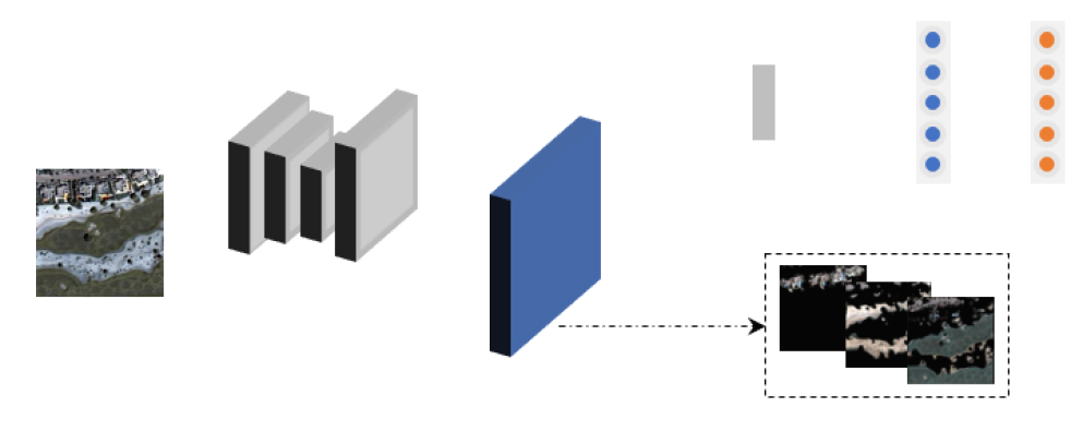
Figure 2: The SPSS (SP-based semantic segmentation) architecture. In the training stage, features are firstly extracted by a CNN from the input; and then the extracted features are through a GAP layer calculating the SP. After training using the loss function $\mathcal{L}_{\rm sp}$, the proposed SPSS architecture can force the extracted features to be the prediction of the class-wise segmentation masks.

The proposed SP-based semantic segmentation (SPSS) architecture is shown in Figure 2. It contains two main parts, see below.

The first part of the SPSS architecture is feature extraction. Employing a convolutional neural network (CNN) is a common approach in current state-of-the-art semantic segmentation methods. In our SPSS, a CNN (or other type of DNNs) is utilised as its backbone to extract high-level image features $\boldsymbol{Y}_{i}$ from the input image $\boldsymbol{X}_{i}$. The second part of the SPSS architecture is a global average pooling (GAP) layer, which takes the image features $\boldsymbol{Y}_{i}$ to generate the SP, $\boldsymbol{\rho}_{i}$, for the input image $\boldsymbol{X}_{i}$. The SPSS architecture is then trained by using the loss function $\mathcal{L}_{\rm sp}$ defined in Eq. (1). After training the SPSS architecture, the extracted features $\boldsymbol{Y}_{i}$ of the trained CNN are, surprisingly, the prediction of the class-wise segmentation masks; that is how the SPSS architecture performs semantic segmentation by just using the SP rather than the ground-truth segmentation maps.

We remark that both parts in the SPSS architecture are well-known and commonly employed for e.g. computer vision tasks. To the best of our knowledge, it is, for the first time, to combine these two parts for semantic segmentation in order to reduce the need of labour-intensive (fine-grained) ground-truth segmentation masks to the (coarse-grained) SP level.

2.2 Architecture Enhancement

The proposed SPSS architecture in Figure 2 only uses the SP annotation for semantic segmentation, which is quite cheap in terms of annotation generation. Moreover, SPSS is also very flexible, i.e., it can be enhanced straightforwardly when additional annotation information is available. Below we give a showcase regarding how to involve several annotated semantic keypoints for some semantic classes (e.g. the minority classes) to enhance the SPSS architecture, see Figure 3. For ease of reference, we call the enhanced architecture in Figure 3 SPSS+.

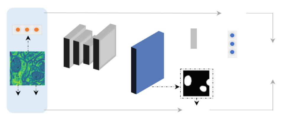
Figure 3: The SPSS+ architecture (cf. the SPSS architecture in Figure 2). In the training stage, features are firstly extracted by a CNN from the input; and then the extracted features are through a GAP layer calculating the SP. After training using the loss function $\mathcal{L}_{\rm total}$ (see Eq. (4)), the SPSS+ architecture can force the extracted features to be the prediction of the class-wise segmentation masks.

Let $\Lambda^{ij}\in[1,M]\times[1,H]$ be the set containing a few number of annotated semantic keypoints for the $j$-th semantic class of image $\boldsymbol{X}_{i}$, i.e., additional annotation information against the SP. We remark that the semantic keypoints in $\Lambda^{ij}$ could be the ones after dilation from for example only two or three semantic keypoints given by experts. Let ${\Omega}_{\rm sk}\subset\mathbb{N}$ be the set containing the indexes of the images in ${\cal X}_{\rm T}$ which have annotated semantic keypoints and ${\Omega}_{\rm sc}^{i}\subset\mathbb{N}$ be the set containing the indexes of the semantic classes with annotated semantic keypoints for image $\boldsymbol{X}_{i}$. Note that in this case limited additional annotation information indicates $|{\Omega}_{\rm sk}|\ll|{\cal X}_{\rm T}|$ and ${\Omega}_{\rm sc}^{i}\ll C$ for most $i\in{\Omega}_{\rm sk}$. Below we define a new loss, $\mathcal{L}_{\rm sk}$, for the annotated semantic keypoints, i.e.,

$$\mathcal{L}_{\rm sk}=\sum_{i\in{\Omega}_{\rm sk}}\sum_{j\in{\Omega}_{\rm sc}^{i}}\sum_{(m,h)\in\Lambda^{ij}}f_{ij}(m,h)/|\Lambda^{ij}|,$$ (3)

where $f_{ij}(m,h)$ is defined in Eq. (2). Finally, the total loss for the SPSS+ architecture is

$$\mathcal{L}_{\rm total}=\alpha\mathcal{L}_{\rm sp}+(1-\alpha)\mathcal{L}_{\rm sk},$$ (4)

where $\alpha$ is an adjustable weight to determine the trade-off between the loss $\mathcal{L}_{\rm sp}$ and loss $\mathcal{L}_{\rm sk}$.

The SPSS+ architecture (in Figure 3) uses the loss $\mathcal{L}_{\rm total}$, which considers the annotations of the SP and semantic keypoints, to train the CNN backbone. Similar to the SPSS architecture (in Figure 2), the extracted features $\boldsymbol{Y}_{i}$ of the trained CNN in the SPSS+ architecture are the prediction of the class-wise segmentation masks, i.e., the semantic segmentation results.

Our SPSS can generally achieve comparable performance against benchmark semantic segmentation methods. Moreover, we find that for quite challenging semantic segmentation problems for example the ones with severe semantic class imbalance, our SPSS+ can still perform effectively. Please see Section 3 for more details regarding validation and comparison.

3 Experiments

The proposed SP-based methodology for semantic segmentation is trained and tested on two benchmark datasets. The details of the data, implementation and experimental results are given below.

Data. Satellite images of Dubai, i.e., Aerial Dubai, is an open-source aerial imagery dataset presented as part of a Kaggle competition. The dataset includes 8 tiles and each tile has 9 images of various sizes and their corresponding ground-truth segmentation masks for 6 classes, i.e., building, land, road, vegetation, water and unlabeled. The other dataset used in this work is the Electron Microscopy dataset, which is a binary segmentation problem and contains 165 slices of microscopy images with the size of $768\times 1024$. The primary aim for this medical dataset is to identify and classify mitochondria pixels. This dataset is quite challenging since its semantic classes are severely imbalanced, i.e., the size of the mitochondria in most slices is very small (e.g. see Figure 6).

Implementation setup.

• Both datasets include large images. They are cropped into smaller patches and we obtain 1647 patches of size $224\times 224\times 3$ and 1980 patches of size $256\times 256$ for the Aerial Dubai and Electron Microscopy datasets, respectively.

• The CNN backbone utilised in our SPSS and SPSS+ architectures is a modified version of U-Net [24], which involves four blocks in the contracting path with increased size of filters. Each block has two convolutional layers with $3\times 3$ filters and ReLU activation. Each block then reduces the size of its input to half by a $2\times 2$ max-pooling layer. The expansive path also has four blocks but with decreased size of filters. Each block involves two transpose convolution layers with a $3\times 3$ filter and ReLU activation. There are also four concatenation operations that stack the resulting components of each of the four blocks in the contracting path with its same-size counterpart in the expansive path. Finally, a $1\times 1$ convolutional layer with $n$ filters and softmax activation are employed to match the $C$ number of the semantic classes. Thus $n$ is set to 6 and 1 to output feature maps of the size $224\times 224\times 6$ and $256\times 256\times 1$ respectively for the Aerial Dubai and Electron Microscopy datasets. Note that there is no need to set $n$ to 2 for the binary segmentation problem dataset Electron Microscopy.

• A GAP layer is then applied to these resulting feature maps to obtain 6 and 1 values, i.e., predicted SP, for the Aerial Dubai and Electron Microscopy datasets, respectively. To obtain segmentation maps during the test stage, we extract the feature maps prior to the GAP layer and visualise them per semantic class (see e.g. Figure 5 for visualisation).

• For all experiments, an 80/20 split for the training/test, Adam optimizer with a learning rate of $10^{-3}$, and a batch size of 16 are chosen. The number of epochs is set to 100 with early stopping applied with patience set to 10 based on the validation loss. All the experiments were implemented on a personal laptop with the following specifications: i7-8750H CPU, GeForce GTX 1060 GPU and 16GB RAM. Training of SPSS and SPSS+ takes around 30 minutes and 20 minutes, respectively.

We emphasise that our main aim here is to show that semantic segmentation can be achieved with significantly weaker annotations, i.e., the SP annotation. We do not focus on performance improvement compared to the benchmark method, i.e., the CNN backbone (i.e., U-Net [24]) trained end-to-end for semantic segmentation using the ground-truth segmentation masks, which are generally much more expensive to annotate compared to the SP that our proposed SPSS and SPSS+ methods utilise. To make fair comparison, the same training images are used to train all the models. Given our limited resources, the image sizes mentioned above are the biggest we could try when the batch size is set to 16. Therefore, all the models are likely to improve their performances with bigger image sizes and hyper-parameter fine-tuning.

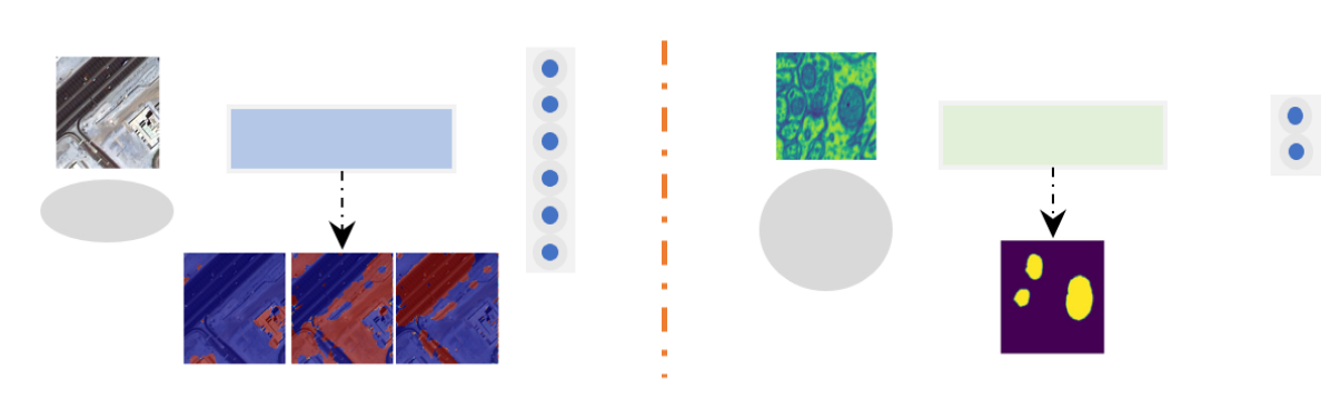
Figure 4: Diagrams of the proposed models SPSS and SPSS+ on the datasets Aerial Dubai (left) and Electronic Microscopy (right), respectively.

Note again that the difference between SPSS and SPSS+ is just the way of using the annotations for their training, i.e., SPSS+ is to address the scenario that (except for the SP) a little more cheap annotations are available. Figure 4 illustrates the difference by utilising the SPSS and SPSS+ architectures on the datasets Aerial Dubai and Electronic Microscopy, respectively.

3.1 Semantic Segmentation Performance Comparison

Quantitative comparison. Table 1 and Table 2 give the quantitative results of our method and the benchmark method for the Aerial Dubai and Electron Microscopy datasets, respectively. Well-known evaluation metrics, i.e., mean intersection over union (Mean IoU) scores, per-class F1 scores and mean accuracy, are employed. Variances are obtained by training the models three times with randomly initialised weights. Tables 1 and 2 show that our model performs comparably to the benchmark segmentation method in both tasks; particularly for the challenging Electron Microscopy dataset, the mean accuracy of our method is just $\sim 1\%$ less than that of the benchmark method, demonstrating the great performance of our methods and the rightfulness of utilising the SP annotation for semantic segmentation that our methodology introduces.

Table 1: Quantitative semantic segmentation results on the Aerial Dubai dataset.

Model	Mean IoU	Per-class F1 score					Mean
		Building	Land	Road	Vegetation	Water	accuracy
Benchmark	$52.3\pm 1.3$	$75.2\pm 0.9$	$84.5\pm 1.3$	$68.3\pm 1.2$	$67.7\pm 0.6$	$90.1\pm 0.4$	$82.3\pm 0.5$
SPSS (ours)	$45.4\pm 0.9$	$63.5\pm 1.1$	$85.4\pm 0.8$	$46.1\pm 1.1$	$61.2\pm 0.8$	$89.5\pm 0.5$	$75\pm 0.7$

Table 2: Quantitative semantic segmentation results on the Electron Microscopy dataset.

Model	Mean IoU	Per-class F1 score		Mean
		Background	Mitochondria	accuracy
Benchmark	$69.2\pm 0.3$	$99.1\pm 0.2$	$81.3\pm 0.5$	$98.4\pm 0.2$
SPSS+ (ours)	$65.3\pm 0.8$	$98.1\pm 0.8$	$79.3\pm 0.3$	$97.7\pm 0.8$

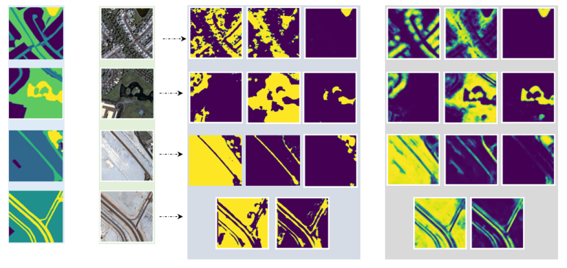
Figure 5: Qualitative semantic segmentation comparison between our SPSS method (middle) and the benchmark method (right) on the Aerial Dubai dataset.

Qualitative comparison. Figure 5 shows the qualitative results of our method and the benchmark method for the Aerial Dubai dataset. Surprisingly, the class-wise segmentation maps that our method achieves (middle of Figure 5) are visually significantly better than that of the benchmark method (right of Figure 5) in terms of the binarisation ability, indicating the effectiveness of the loss $\mathcal{L}_{\rm sp}$ (defined in Eq. (1)) using the SP annotation introduced in our method.

For the significant class imbalance dataset Electronic Microscopy, Figure 6 shows the qualitative results of our method and the benchmark method for some challenging cases. Again, our method exhibits superior performance against the benchmark method. For example, our method accurately segments the mitochondria on the top-left corner of the second image despite employing much less annotation, but the benchmark method completely misses it even though trained using the ground-truth segmentation masks. This again validates the rightfulness of utilising the SP annotation for semantic segmentation that our methodology introduces. Most importantly, due to the great binarisation ability of the loss function introduced in our method using SP, it may serve as auxiliary loss even in scenarios where ground-truth segmentation masks are available so as to enhance the semantic segmentation performance of many existing methods.

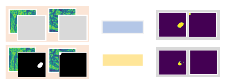
Figure 6: Qualitative semantic segmentation comparison between our SPSS+ method (upper) and the benchmark method (lower) on some images from the Electronic Microscopy dataset.

3.2 Sensitivity Analysis

The task of obtaining highly precise SP annotations may be challenging, and as a result, annotators may provide rough estimates instead. Below we investigate the robustness of our models corresponding to the quality of the SP. Two extreme ways degrading the SP are examined, i.e., one is adding noises to the SP directly and the other is assigning images in individual clusters the same SP.

Table 3: Performance of our model trained by using the SP degraded by Gaussian noise.

Data	Noise (%)	Mean IoU
	0	45
	5	42
	10	41
Aerial	15	38
Dubai	20	32
	30	29
	40	28
	50	26

SP degraded by Gaussian noise. We firstly conduct the sensitivity analysis of our method by systematically adding Gaussian noise to the SP. Let $\mathcal{N}(0,\sigma)$ be the normal distribution with 0 mean and standard deviation $\sigma$. For the given ST $\boldsymbol{\rho}^{*}_{i}=(\rho^{*}_{i1},\cdots,\rho^{*}_{iC})$ of $\forall\boldsymbol{X}_{i}\in{\cal X}_{\rm T}$, let $\boldsymbol{\tilde{\rho}}^{*}_{i}=(\tilde{\rho}^{*}_{i1},\cdots,\tilde{\rho}^{*}_{iC})$, where

$$\tilde{\rho}^{*}_{ij}=\rho^{*}_{ij}+\mathcal{N}(0,\sigma),\ \ j=1,\cdots,C.$$ (5)

Then the softmax operator is used to normalise $\boldsymbol{\tilde{\rho}}^{*}_{i}$, and the normalised $\boldsymbol{\tilde{\rho}}^{*}_{i}$ is used as the new ST to train our model. Here the standard deviation $\sigma$ controls the level of the Gaussian noise being added to the ST; e.g. $\sigma=0.1$ represents $10\%$ Gaussian noise.

Table 3 showcases the robustness of our methodology, as it continues performing well even with the SP degraded by quite high levels of noise; e.g., the Mean IOU our method achieves only drops $4\%$ for $10\%$ Gaussian noise being added to the SP. Our method can still work to some extent even with the SP degraded by $50\%$ Gaussian noise. This shows that our method is indeed quite robust corresponding to the SP, which means the annotators could in practice spend much less effort for providing rough SP rather than the precise SP.

Table 4: Performance of our model trained by using the SP degraded by clustering.

Data	# Clusters	Mean IoU
	100	44
	50	42
Aerial	30	41
Dubai	20	37
	10	36
	5	27

SP degraded by clustering. We now conduct the sensitivity analysis of our method by degrading the SP of the training images by clustering. The degradation procedures are: i) clustering the set of the given ST, i.e., $\{\boldsymbol{\rho}^{*}_{i}\}_{i\in{\Omega}_{\rm T}}$, into $K$ clusters by $K$-means; ii) clustering the training set ${\cal X}_{\rm T}$ into the same $K$ clusters, say ${\cal X}_{\rm T}^{k},k=1,\ldots,K$, corresponding to the ST clusters; and iii) assigning all the training images in cluster ${\cal X}_{\rm T}^{k}$ the same SP which is randomly selected from the SP of one image in this cluster; see also Figure 7 for illustration. Obviously, implementing this way of degrading the SP, all the images’ SP in the training set ${\cal X}_{\rm T}$ are changed except for $K$ (i.e., the number of clusters) images. The smaller the number $K$, the severer the ST degradation.

The performance of our method regarding the ST degraded by clustering is shown in Table 4, indicating again the robustness of our methodology corresponding to the SP. For example, after just using $K=100$ images’ SP for the whole training set ${\cal X}_{\rm T}$, the Mean IoU of our method only drops 1%; and just using $K=5$ images’ SP for the whole training set, our method can still work to some extent (i.e., the Mean IoU just drops less than half). This again shows that our method is indeed quite robust corresponding to the SP. Most importantly, this also inspires us that the annotators could in practice just provide rough SP for some representative images from the whole training set rather than the SP for the whole training set, which will further significantly reduce the annotation effort.

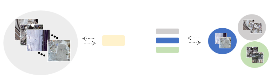
Figure 7: Diagram of the SP annotation degraded by clustering. Images are clustered corresponding to the SP clusters which are achieved by applying $K$-means on the SP set. An SP annotation for one image in each image cluster is then randomly selected from that cluster and is assigned to all the images in that image cluster. Therefore, after degradation, only $K$ images have their original SP annotation if we assume every training image has different SP annotation in the original SP set.

4 Discussion and Limitations

SP (semantic proportions). SP for each training image is required as annotation/label information for the presented semantic segmentation model. In this work, we obtained these proportions from the segmentation maps available for the chosen datasets just to demonstrate the effectiveness and robustness of our proposed SP-based methodology. We would like to stress that the reason why we benefited from the existing segmentation maps, which seems controversial to our main aim at first glance, is to show that the proposed methodology is feasible in the presence of SP. Arguably, the most accurate proportions can be extracted from these ground-truth segmentation maps if they are annotated properly. Therefore, obtaining SP from the readily available maps to achieve our aim is sensible. Clearly, our goal is to train our proposed model when the segmentation maps are unavailable. It is evident that obtaining SP annotation could be much cheaper than obtaining the precise segmentation maps particularly for data volumes in high dimensions for example. There are various ways to obtain SP readily in the absence of the segmentation maps, such as by employing mechanical turks or utilising pre-trained large language models, e.g., ChatGPT [20].

The results that we present in Section 3 are promising and one may wonder if the exact proportions are a must, which would make the proposed setting as expensive as the traditional one. To demonstrate that it is not the case and that our methodology only needs rough SP, we presented sensitivity analysis regarding SP, where we added various amounts of noise to the extracted SP and demonstrated that the model performs satisfactorily well when trained with noisy SP. We also presented sensitivity analysis through investigating degraded SP by clustering to further support the robustness of our methodology when the precise SP is unavailable. The analysis inspires us that our methodology not only works well with rough SP, but also with rough SP for only some representative images from the whole training set, indicating its need of significantly less annotation effort.

Additional annotations. In many scenarios, different types of annotations may exist. This raises the question that whether it is feasible for semantic segmentation methods to use the combination of different types of annotations to boost their performance. In this regard, our proposed semantic segmentation methodology based on SP delivers quite promising results.

For datasets where the ground-truth segmentation maps are available, based on which the SP annotation can be calculated directly. This way naturally augments the annotation types from one to two already. Our proposed model, i.e., SPSS+, can directly utilise both annotation types. The results shown in Section 3 on the Electron Microscopy dataset (with significant class imbalance) demonstrated the great performance of SPSS+ by just using several annotated points from the full ground-truth segmentation maps. The enhanced performance of our method by utilising both annotation types may benefit from our introduced loss function $\mathcal{L}_{\rm total}$ in Eq. (4). It contains the $\mathcal{L}_{\rm sp}$ loss defined in Eq. (1), which measures the MSE between the predicted SP and the given SP. The visualisation results in Figure 5 showed that our $\mathcal{L}_{\rm sp}$ loss is much better than the loss directly measuring the segmentation maps (that the benchmark method uses) in terms of the binarisation ability. Therefore, combining the $\mathcal{L}_{\rm sp}$ loss with the $\mathcal{L}_{\rm sk}$ loss and then forming the $\mathcal{L}_{\rm total}$ loss could boost the semantic segmentation performance, e.g. see the visualisation given in Figure 6.

On the whole, we in this work proposed a new semantic segmentation methodology by introducing the SP annotation. In the scenario of quite limited annotation, using SP for semantic segmentation can already achieve competitive results. If additional annotations are available, our method can easily utilise them for performance boost. On the other hand, for existing segmentation methods that use different types of annotations, we also suggest involving SP in these methods; e.g., our proposed $\mathcal{L}_{\rm sp}$ loss could be served as a type of regularisation given its effectiveness in binarisation.

5 Related Work

Supervision levels in semantic segmentation. In recent years, more and more researchers have focused on reducing the annotation cost for semantic segmentation tasks. One such approach is to use weakly supervised learning techniques that require less precise or less expensive forms of supervision. For instance, Wei et al. [26] proposed a method that utilises image-level labels, the work in [22, 8] uses bounding boxes, and the methods in [15, 14] feed scribbles as labels instead of precise annotations to conduct semantic segmentation. Those approaches can significantly reduce the annotation cost, as they require less manual effort to annotate the data. However, there is always a trade-off between the annotation cost and the model performance, i.e., models trained with higher levels of supervision generally perform better than weakly supervised models.

Active learning is an alternative approach to reduce the annotation cost by selecting the most informative samples to annotate based on the current model’s uncertainty. With the selected most informative samples, active learning can reduce the amount of data that needs to be labelled, thus reducing the annotation cost [19, 27]. It is worth mentioning that this is actually similar to the way we used for the SP degraded by clustering. Reducing the annotation cost could also be achieved by generating synthetic data that can be used to augment the real-world data [7]. Synthetic data can be generated using e.g. computer graphics or other techniques to simulate realistic images and labels.

DNNs for semantic segmentation. Long et al. [16] made a breakthrough by proposing the fully convolutional networks (FCNs) for semantic segmentation. The FCNs utilise CNN to transform input images into a probability map, where each entry of the probability map represents the likelihood of the corresponding image pixel belonging to a particular class. This approach allows the model to learn spatial features and eliminate the need for hand-crafted features. Following FCN, several variants have been proposed to improve the segmentation performance. For example, SegNet [2] is a modification of FCN employing an encoder-decoder architecture to achieve better performance; and DeepLab [6] introduced a novel technique called atrous spatial pyramid pooling to capture multi-scale information from the input image.

U-Net [24], the backbone used in our proposed methodology, is a type of CNN consisting of a contracting path and an expansive path. The skip connections in U-Net allow the network to retain and reuse high-level feature representations learned in the contracting path, helping to improve segmentation accuracy. The U-Net architecture has been widely used for biomedical image segmentation tasks such as cell segmentation [13], organ segmentation [5] and lesion detection [9, 4], due to its ability in accurately segmenting objects within images while using relatively fewer training samples. Furthermore, its modular architecture and efficient training make it adaptable to a wide range of segmentation tasks. Therefore, to demonstrate our methodology utilising SP, we employ a modified and relatively basic version of the U-Net architecture as the backbone of our models.

6 Conclusion

Semantic segmentation methodologies generally require costly annotations such as the ground-truth segmentation masks in order to achieve satisfying performance. Motivated by reducing the annotation time and cost for semantic segmentation, we in this paper presented a new methodology – SPSS – which relies on the SP annotation instead of the costly ground-truth segmentation maps. Extensive experiments validated the great potential of the proposed methodology in reducing the time and cost required for annotation, making it more feasible for large-scale applications. Furthermore, this innovative design opens up new opportunities for semantic segmentation tasks where obtaining the full ground-truth segmentation maps may not be feasible or practical. We believe that the use of the SP annotation suggested in this paper offers a new and promising avenue for future research in the field of semantic segmentation, and wide real-world applications are evident.

References

- [1] Saeid Asgari Taghanaki, Kumar Abhishek, Joseph Paul Cohen, Julien Cohen-Adad, and Ghassan Hamarneh. Deep semantic segmentation of natural and medical Images: a review. Artificial Intelligence Review, 54:137–178, 2021.
- [2] Vijay Badrinarayanan, Alex Kendall, and Roberto Cipolla. Segnet: A Deep Convolutional Encoder-decoder Architecture for Image Segmentation. IEEE transactions on pattern analysis and machine intelligence, 39(12):2481–2495, 2017.
- [3] Amy Bearman, Olga Russakovsky, Vittorio Ferrari, and Li Fei-Fei. What’s the Point: Semantic Segmentation with Point Supervision. In European conference on computer vision, pages 549–565. Springer, 2016.
- [4] Yufeng Cao, April Vassantachart, C Ye Jason, Cheng Yu, Dan Ruan, Ke Sheng, Yi Lao, Zhilei Liu Shen, Salim Balik, Shelly Bian, et al. Automatic detection and segmentation of multiple brain metastases on magnetic resonance image using asymmetric UNet architecture. Physics in Medicine & Biology, 66(1):015003, 2021.
- [5] Hao Chen, Wen Zhang, Xiaochao Yan, Yanbin Chen, Xin Chen, Mengjun Wu, Lin Pan, and Shaohua Zheng. Multi-organ Segmentation Based on 2.5D Semi-supervised Learning. In Fast and Low-Resource Semi-supervised Abdominal Organ Segmentation: MICCAI 2022 Challenge, FLARE 2022, Held in Conjunction with MICCAI 2022, Singapore, September 22, 2022, Proceedings, pages 74–86. Springer, 2023.
- [6] Liang-Chieh Chen, George Papandreou, Iasonas Kokkinos, Kevin Murphy, and Alan L Yuille. Deeplab: Semantic Image Segmentation with Deep Convolutional Nets, Atrous Convolution, and Fully Connected CRFs. IEEE transactions on pattern analysis and machine intelligence, 40(4):834–848, 2017.
- [7] Yuhua Chen, Wen Li, Xiaoran Chen, and Luc Van Gool. Learning Semantic Segmentation from Synthetic data: A Geometrically Guided Input-output Adaptation Approach. In Proceedings of the IEEE/CVF conference on computer vision and pattern recognition, pages 1841–1850, 2019.
- [8] Jifeng Dai, Kaiming He, and Jian Sun. Boxsup: Exploiting Bounding Boxes to Supervise Convolutional Networks for Semantic Segmentation. In Proceedings of the IEEE international conference on computer vision, pages 1635–1643, 2015.
- [9] Mehwish Dildar, Shumaila Akram, Muhammad Irfan, Hikmat Ullah Khan, Muhammad Ramzan, Abdur Rehman Mahmood, Soliman Ayed Alsaiari, Abdul Hakeem M Saeed, Mohammed Olaythah Alraddadi, and Mater Hussen Mahnashi. Skin Cancer Detection: a Review Using Deep Learning Techniques. International journal of environmental research and public health, 18(10):5479, 2021.
- [10] Alberto Garcia-Garcia, Sergio Orts-Escolano, Sergiu Oprea, Victor Villena-Martinez, and Jose Garcia-Rodriguez. A Review on Deep Learning Techniques Applied to Semantic Segmentation. arXiv preprint arXiv:1704.06857, 2017.
- [11] Kyle Genova, Xiaoqi Yin, Abhijit Kundu, Caroline Pantofaru, Forrester Cole, Avneesh Sud, Brian Brewington, Brian Shucker, and Thomas Funkhouser. Learning 3D Semantic Segmentation with Only 2D Image Supervision. In 2021 International Conference on 3D Vision (3DV), pages 361–372. IEEE, 2021.
- [12] Shijie Hao, Yuan Zhou, and Yanrong Guo. A Brief Survey on Semantic Segmentation with Deep Learning. Neurocomputing, 406:302–321, 2020.
- [13] Haigen Hu, Yixing Zheng, Qianwei Zhou, Jie Xiao, Shengyong Chen, and Qiu Guan. MC-Unet: Multi-scale Convolution Unet for Bladder Cancer Cell Segmentation in Phase-contrast Microscopy Images. In 2019 IEEE International Conference on Bioinformatics and Biomedicine (BIBM), pages 1197–1199. IEEE, 2019.
- [14] Hyeonsoo Lee and Won-Ki Jeong. Scribble2label: Scribble-supervised Cell Segmentation via Self-generating Pseudo-labels with Consistency. In Medical Image Computing and Computer Assisted Intervention–MICCAI 2020: 23rd International Conference, Lima, Peru, October 4–8, 2020, Proceedings, Part I 23, pages 14–23. Springer, 2020.
- [15] Di Lin, Jifeng Dai, Jiaya Jia, Kaiming He, and Jian Sun. Scribblesup: Scribble-supervised Convolutional Networks for Semantic Segmentation. In Proceedings of the IEEE conference on computer vision and pattern recognition, pages 3159–3167, 2016.
- [16] Jonathan Long, Evan Shelhamer, and Trevor Darrell. Fully Convolutional Networks for Semantic Segmentation. In Proceedings of the IEEE conference on computer vision and pattern recognition, pages 3431–3440, 2015.
- [17] R Austin McEver and BS Manjunath. Pcams: Weakly Supervised Semantic Segmentation Using Point Supervision. arXiv preprint arXiv:2007.05615, 2020.
- [18] Andres Milioto, Philipp Lottes, and Cyrill Stachniss. Real-time Semantic Segmentation of Crop and Weed for Precision Agriculture Robots Leveraging Background Knowledge in CNNs. In 2018 IEEE international conference on robotics and automation (ICRA), pages 2229–2235. IEEE, 2018.
- [19] Sudhanshu Mittal, Joshua Niemeijer, Jörg P Schäfer, and Thomas Brox. Revisiting Deep Active Learning for Semantic Segmentation. arXiv preprint arXiv:2302.04075, 2023.
- [20] OpenAI. Introducing ChatGPT. https://openai.com/blog/chatgpt, 2022.
- [21] Dim P Papadopoulos, Alasdair DF Clarke, Frank Keller, and Vittorio Ferrari. Training Object Class Detectors from Eye Tracking Data. In Computer Vision–ECCV 2014: 13th European Conference, Zurich, Switzerland, September 6-12, 2014, Proceedings, Part V 13, pages 361–376. Springer, 2014.
- [22] George Papandreou, Liang-Chieh Chen, Kevin P Murphy, and Alan L Yuille. Weakly-and Semi-supervised Learning of a Deep Convolutional Network for Semantic Image Segmentation. In Proceedings of the IEEE international conference on computer vision, pages 1742–1750, 2015.
- [23] Pedro O Pinheiro and Ronan Collobert. From Image-level to Pixel-level Labeling with Convolutional Networks. In Proceedings of the IEEE conference on computer vision and pattern recognition, pages 1713–1721, 2015.
- [24] Olaf Ronneberger, Philipp Fischer, and Thomas Brox. U-net: Convolutional Networks for Biomedical Image Segmentation. In Medical Image Computing and Computer-Assisted Intervention–MICCAI 2015: 18th International Conference, Munich, Germany, October 5-9, 2015, Proceedings, Part III 18, pages 234–241. Springer, 2015.
- [25] Mennatullah Siam, Mostafa Gamal, Moemen Abdel-Razek, Senthil Yogamani, Martin Jagersand, and Hong Zhang. A Comparative Study of Real-time Semantic Segmentation for Autonomous Driving. In Proceedings of the IEEE conference on computer vision and pattern recognition workshops, pages 587–597, 2018.
- [26] Yunchao Wei, Xiaodan Liang, Yunpeng Chen, Zequn Jie, Yanhui Xiao, Yao Zhao, and Shuicheng Yan. Learning to Segment with Image-level Annotations. Pattern Recognition, 59:234–244, 2016.
- [27] Shuai Xie, Zunlei Feng, Ying Chen, Songtao Sun, Chao Ma, and Mingli Song. Deal: Difficulty-aware Active Learning for Semantic Segmentation. In Proceedings of the Asian conference on computer vision, 2020.
- [28] Ruixin Yang and Yingyan Yu. Artificial Convolutional Neural Network in Object Detection and Semantic Segmentation for Medical Imaging Analysis. Frontiers in oncology, 11:638182, 2021.
- [29] Huanle Zhang, Bo Han, Cheuk Yiu Ip, and Prasant Mohapatra. Slimmer: Accelerating 3D Semantic Segmentation for Mobile Augmented Reality. In 2020 IEEE 17th International Conference on Mobile Ad Hoc and Sensor Systems (MASS), pages 603–612. IEEE, 2020.