Linear Neural Network Layers Promote Learning Single- and Multiple-Index Models

Abstract

This paper explores the implicit bias of overparameterized neural networks of depth greater than two layers. Our framework considers a family of networks of varying depths that all have the same capacity but different implicitly defined representation costs. The representation cost of a function induced by a neural network architecture is the minimum sum of squared weights needed for the network to represent the function; it reflects the function space bias associated with the architecture. Our results show that adding linear layers to a ReLU network yields a representation cost that favors functions that can be approximated by a low-rank linear operator composed with a function with low representation cost using a two-layer network. Specifically, using a neural network to fit training data with minimum representation cost yields an interpolating function that is nearly constant in directions orthogonal to a low-dimensional subspace. This means that the learned network will approximately be a single- or multiple-index model. Our experiments show that when this active subspace structure exists in the data, adding linear layers can improve generalization and result in a network that is well-aligned with the true active subspace.

1 Introduction

An outstanding problem in understanding the generalization properties of overparameterized neural networks is characterizing which functions are best represented by neural networks of varying architectures. Past work explored the notion of representation costs – i.e., how much does it “cost” for a neural network to represent some function $f$. Specifically, the representation cost of a function $f$ is the minimum sum of squared network weights necessary for the network to represent $f$.

The following key question then arises: How does network architecture affect which functions have minimum representation cost? In this paper, we describe the representation cost of a family of networks with $L$ layers in which $L-1$ layers have linear activations and the final layer has a ReLU activation. As detailed in § 1.1, networks related to this class play an important role in both theoretical studies of neural network generalization properties and experimental efforts.

For instance, imagine training a neural network to interpolate a set of training samples using weight decay; the corresponding interpolant will have minimal representation cost, and so the network architecture will influence which interpolating function is learned. This can have a profound effect on test performance, particularly outside the domain of the training samples.

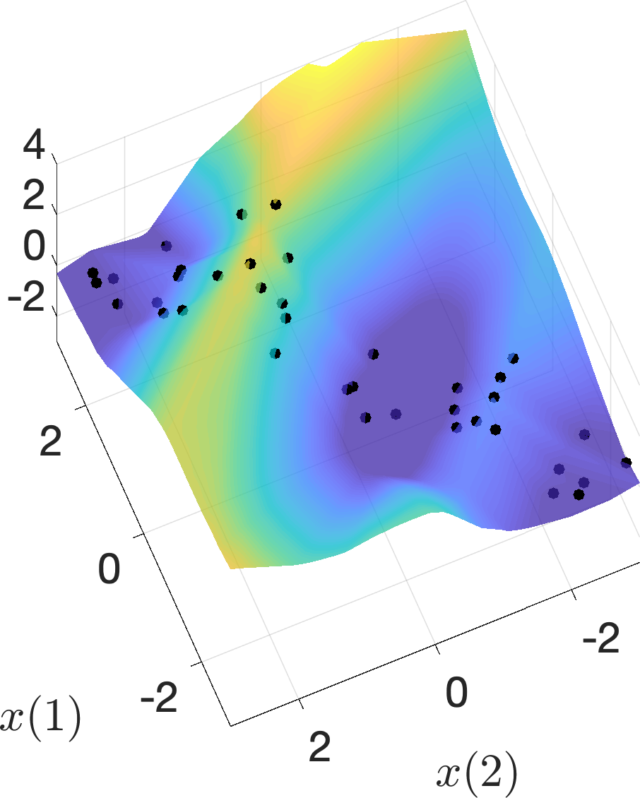
(a) $L=2$ layers

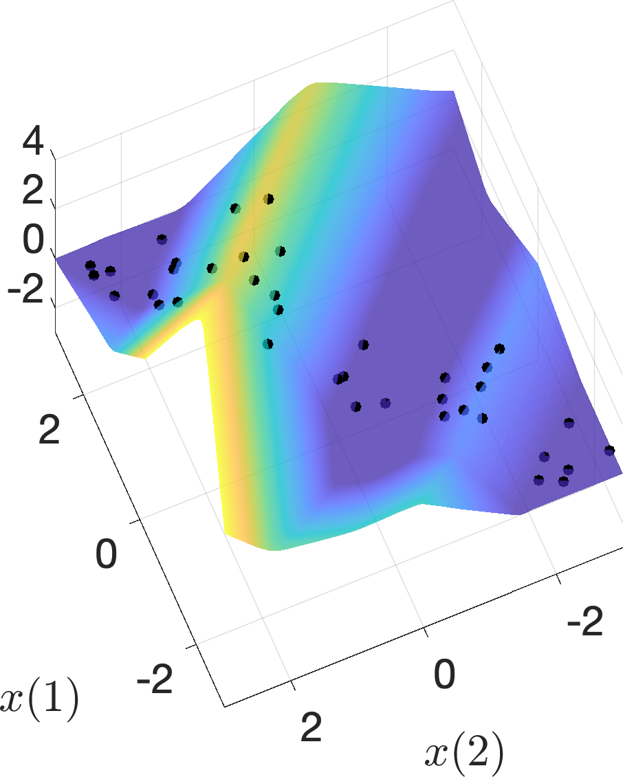
(b) $L=3$ layers

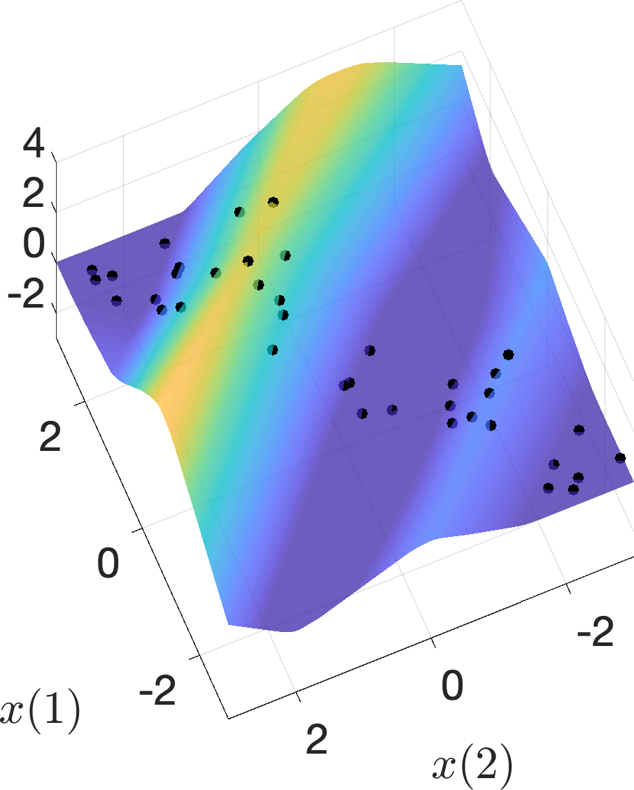
(c) $L=4$ layers

Figure 1: Numerical evidence that weight decay promotes unit alignment with more linear layers. Neural networks with $L-1$ linear layers plus one ReLU layer were trained using SGD with weight decay regularization to close to zero training loss on the training samples, as shown in black. Pictured in (a)-(c) are the resulting interpolating functions shown as surface plots. Our theory predicts that as the number of linear layers increases, the learned interpolating function will become closer to constant in directions perpendicular to a low-dimensional subspace on which a parsimonious interpolant can be defined.

This paper characterizes the representation cost of deep neural networks with linear layers. Our bounds, which depend on the “rank” of the function, highlight the role that depth plays in model selection. Our notion of a function’s rank has close connections to multi- and single-index models, central subspaces, active subspaces, and mixed variation function classes. Unlike related analyses of representation costs and a function’s rank [17], our approach meaningfully reflects latent low-dimensional structure in broad families of functions, including those with scalar outputs. We show that adding linear layers to a ReLU network with weight decay regularization is akin to using a two-layer ReLU network with nuclear or Schatten norm regularization on the weight matrix. This insight suggests that lower-rank weight matrices, corresponding to aligned ReLU units, as illustrated in Figure 1, will be favored. More specifically, we characterize the singular value spectrum of central subspaces associated with learned functions and show that minimizers of the representation cost are nearly rank-1. Numerical experiments reveal that with enough data the learned function’s central subspace closely approximates the central subspace of the data-generating function, which helps improve generalization and out-of-distribution performance.

1.1 Related work

Representation costs

Multiple works have argued that in neural networks, “the size [magnitude] of the weights is more important than the size [number of weights or parameters] of the network” [4, 26, 42]. This perspective gives insight into the generalization performance of overparameterized neural networks. That is, both theory and practice have indicated that generalization is not achieved by limiting the size of the network, but rather by controlling the magnitudes of the weights [37, 25, 22]. As networks are trained, they seek weights with minimal norm required to represent a function that accurately fits the training data. Such minimum norm solutions and the corresponding “representational cost of a function” play an important role in generalization performance. A number of papers have studied representation costs and implicit regularization from a function space perspective associated with neural networks. Following a univariate analysis by Savarese et al., [32], Ongie et al., [27] considers two-layer multivariate ReLU networks where the hidden layer has infinite width. Recent work by Mulayoff et al., [24] connects the function space representation costs of two-layer ReLU networks to the stability of SGD minimizers. Ergen and Pilanci, [11] consider representation costs associated with deep nonlinear networks, but place strong assumptions on the data distribution (i.e., rank-1 or orthonormal training data).

Linear layers

Gunasekar et al., [15] shows that $L$-layer linear networks with diagonal structure induces a non-convex implicit bias over network weights corresponding to the $\ell^{q}$ norm of the outer layer weights for $q=2/L$; similar conclusions hold for deep linear convolutional networks. Recent work by Dai et al., [9] examines the representation costs of deep linear networks from a function space perspective, and Ji and Telgarsky, [18] shows that gradient descent on linear networks produces aligned ReLU. However, the existing literature does not fully characterize the representation costs of deep, non-linear networks from a function space perspective. Parhi and Nowak, [28] consider deeper networks and define a compositional function space with a corresponding representer theorem; the properties of this function space and the role of depth are an area of active investigation.

Our paper focuses on the role of linear layers in nonlinear networks. This is a particularly important family to study because adding linear layers does not change the capacity or expressivity of a network, even though the number of parameters may change. This means that different behaviors for different depths solely reflect the role of depth and not of capacity. The role of linear layers in such settings has been explored in a number of works. Golubeva et al., [14] looks at the role of network width when the number of parameters is held fixed; it specifically looks at increasing the width without increasing the number of parameters by adding linear layers. This procedure seems to help with generalization performance (as long as the training error is controlled). However, Golubeva et al., [14] notes that the implicit regularization caused by this approach is not understood. One of the main contributions of our paper is a better understanding of this implicit regularization.

The effect of linear layers on training speed was previously examined by Ba and Caruana, [3] and Urban et al., [35]. Arora et al., [1] considers implicit acceleration in deep nets and claims that depth induces a momentum-like term in training deep linear networks with SGD, though the regularization effects of this acceleration are not well understood. Implicit regularization of gradient descent has been studied in the context of matrix and tensor factorization problems [15, 2, 30, 31]. Similar to this work, low-rank representations play a key role in their analysis. Linear layers have also been shown to help uncover latent low-dimensional structure in dynamical systems [41].

Single- and multi-index models

Multi-index models are functions of the form

$$f({\bm{x}})=g(\langle{\bm{v}}_{1},{\bm{x}}\rangle,\langle{\bm{v}}_{2},{\bm{x}}\rangle,\ldots,\langle{\bm{v}}_{r},{\bm{x}}\rangle)=g({\bm{V}}^{\top}{\bm{x}})$$ (1)

for some $r$-dimensional subspace spanned by the columns of ${\bm{V}}:=\begin{bmatrix}{\bm{v}}_{1}&\ldots&{\bm{v}}_{r}\end{bmatrix}$ and unknown link function $g:\mathbb{R}^{r}\mapsto\mathbb{R}$. This subspace is called a central subspace in some papers. Single-index models correspond to the special case where $r=1$. Multiple works have explored learning such models (specifically, learning both the basis vectors and the link function) in high dimensions [43, 38, 40, 19, 20, 13, 12]. The link function $g$ has a domain in a $r$-dimensional space, so the sample complexity of learning these models depends primarily on $r$ even when the dimension of ${\bm{x}}$ is large. Specifically, as noted by Liu and Liao, [20], the minimax mean squared error rate for general functions $f$ that are $s$-Hölder smooth is $n^{-\frac{2s}{2s+d}}$, while for functions with a rank-$r$ central subspace, the minimax rate is $n^{-\frac{2s}{2s+r}}$. The difference between these rates implies that for $r\ll d$, a method that can adapt to the central subspace can achieve far lower errors than a non-adaptive method.

Two recent papers [23, 5] explore learning single-index models using shallow neural networks. Unlike this paper, those works force the single-index structure: Bietti et al., [5] by constraining the inner weights of all hidden nodes to have the same weight vector, and Mousavi-Hosseini et al., [23] by initializing all weights to be equal and noting that gradient-based updates of the weights will maintain this symmetry.

1.2 Notation

For a vector ${\bm{a}}\in\mathbb{R}^{K}$, we use $\|{\bm{a}}\|_{p}$ to denote its $\ell^{p}$ norm. For a matrix ${\bm{W}}$, we use $\|{\bm{W}}\|_{op}$ to denote the operator norm, $\|{\bm{W}}\|_{F}$ to denote the Frobenius norm, $\|{\bm{W}}\|_{*}$ to denote the nuclear norm (i.e., the sum of the singular values), and for $0<q\leq 1$ we use $\|{\bm{W}}\|_{\mathcal{S}^{q}}$ to denote the Schatten-$q$ quasi-norm (i.e., the $\ell^{q}$ quasi-norm of the singular values of a matrix ${\bm{W}}$). We let $\sigma_{k}({\bm{W}})$ denote the $k$-th largest singular value of ${\bm{W}}$. Given a vector ${\bm{a}}\in\mathbb{R}^{K}$, the matrix ${\bm{D}}_{{\bm{a}}}\in\mathbb{R}^{K\times K}$ is a diagonal matrix with the entries of ${\bm{a}}$ along the diagonal. For a vector $\bm{\lambda}$, we write $\bm{\lambda}>0$ to indicate it has all positive entries. For the weighted $L_{2}$-norm of a function $f$ with respect to a probability distribution $\rho$ we write $\|f\|_{L_{2}(\rho)}$. Finally, we use $[t]_{+}=\max\{0,t\}$ to denote the ReLU activation, whose application to vectors is understood entrywise.

2 Definitions

Let $\mathcal{X}\subseteq\mathbb{R}^{d}$ be either a bounded convex set with nonempty interior or all of $\mathbb{R}^{d}$. Fix an absolutely continuous probability distribution with density $\rho$ such that $\rho({\bm{x}})>0$ if and only if ${\bm{x}}\in\mathcal{X}$. Let $\mathcal{N}_{2}\left(\mathcal{X}\right)$ denote the space of functions $f:\mathcal{X}\rightarrow\mathbb{R}$ expressible as a two-layer ReLU network having input dimension $d$ and such that the width $K$ of the single hidden layer is unbounded. Every function in $\mathcal{N}_{2}\left(\mathcal{X}\right)$ is described (non-uniquely) by a collection of weights $\theta=({\bm{W}},{\bm{a}},{\bm{b}},c)$:

$$h_{\theta}^{(2)}({\bm{x}}) ={\bm{a}}^{\top}[{\bm{W}}{\bm{x}}+{\bm{b}}]_{+}+c=\sum_{k=1}^{K}a_{k}[{\bm{w}}_{k}^{\top}{\bm{x}}+b_{k}]_{+}+c$$ (2)

with ${\bm{W}}\in\mathbb{R}^{K\times d}$, ${\bm{a}},{\bm{b}}\in\mathbb{R}^{K}$ and $c\in\mathbb{R}$. We denote the set of all such parameter vectors $\theta$ by $\Theta_{2}$.

In this work, we consider a re-parameterization of networks in $\mathcal{N}_{2}\left(\mathcal{X}\right)$. Specifically, we replace the linear input layer ${\bm{W}}$ with $L-1$ linear layers:

$$h_{\theta}^{(L)}({\bm{x}}) ={\bm{a}}^{\top}[{\bm{W}}_{L-1}\cdots{\bm{W}}_{2}{\bm{W}}_{1}{\bm{x}}+{\bm{b}}]_{+}+c$$ (3)

where now $\theta=({\bm{W}}_{1},{\bm{W}}_{2},...,{\bm{W}}_{L-1},{\bm{a}},{\bm{b}},c)$. Again, we allow the widths of all layers to be arbitrarily large. Let $\Theta_{L}$ denote the set of all such parameter vectors. With any $\theta\in\Theta_{L}$ we associate the cost

$$C_{L}(\theta)=\frac{1}{L}\left(\|{\bm{a}}\|_{2}^{2}+\|{\bm{W}}_{1}\|_{F}^{2}+\cdots+\|{\bm{W}}_{L-1}\|_{F}^{2}\right),$$ (4)

i.e., the squared Euclidean norm of all non-bias weights; this cost is equivalent to the “weight decay” penalty [21].

Given training pairs $\{({\bm{x}}_{i},y_{i})\}_{i=1}^{n}$ with ${\bm{x}}_{i}\in\mathcal{X}$, consider the problem of finding an $L$-layer network with minimal cost $C_{L}$ that interpolates the training data:

$$\min_{\theta\in\Theta_{L}}C_{L}(\theta)~{}~{}\mathrm{s.t.}~{}~{}h^{(L)}_{\theta}({\bm{x}}_{i})=y_{i}\;\;\forall i=1,\ldots,n$$ (5)

This optimization is akin to training a network to interpolate training data using SGD with squared $\ell^{2}$ norm or weight decay regularization [16, 21]. We may recast this as an optimization problem in function space: for any $f\in\mathcal{N}_{2}\left(\mathcal{X}\right)$, define its $L$-layer representation cost $R_{L}(f)$ by

$$R_{L}(f)=\inf_{\theta}C_{L}(\theta)~{}~{}\mathrm{s.t.}~{}~{}f=h^{(L)}_{\theta}|_{\mathcal{X}}.$$ (6)

Then (5) is equivalent to:

$$\min_{f\in\mathcal{N}_{2}\left(\mathcal{X}\right)}R_{L}(f)~{}~{}\mathrm{s.t.}~{}~{}f({\bm{x}}_{i})=y_{i}.$$ (7)

Earlier work, such as [32], has shown that the 2-layer representation cost reduces to

$$R_{2}(f)= \inf_{\theta\in\Theta_{2}}\|{\bm{a}}\|_{1}~{}~{}\mathrm{s.t.}~{}~{}\|{\bm{w}}_{k}\|_{2}=1,\qquad\forall k=1,...,K~{}\text{and}~{}f=h^{(2)}_{\theta}$$ (8)

Our goal is to characterize the representation cost $R_{L}$ for different numbers of linear layers $L\geq 3$, and describe how the set of global minimizers of (7) changes with $L$, providing insight into the role of linear layers in nonlinear ReLU networks.

3 Low-rank and mixed variation functions

We will see that adding linear layers promotes selecting “low-rank” functions to fit the training data. In this section, we formalize the notion of low-rank and mixed variation functions as well as their connections to related concepts in the literature.

3.1 Low-rank functions and active subspaces

We define the rank of a function using its active subspace [8, 7]. The idea is to identify a linear subspace corresponding to directions of large variation in a function using a PCA-like technique applied to the uncentered covariance matrix of the gradient. Consider the uncentered covariance matrix of the gradient of a function $f:\mathcal{X}\rightarrow\mathbb{R}$:

$${\bm{C}}_{f,\rho}:=\mathbb{E}_{\rho}[\nabla f({\bm{x}})\nabla f({\bm{x}})^{\top}]=\int_{\mathcal{X}}\nabla f({\bm{x}})\nabla f({\bm{x}})^{\top}\rho({\bm{x}})\,d{\bm{x}}.$$ (9)

Note that $f$ is constant in the direction of an eigenvector of ${\bm{C}}_{f,\rho}$ with zero eigenvalue, and nearly constant in the direction of an eigenvector with small eigenvalue. To see this, observe that the Rayleigh quotients with respect to ${\bm{C}}_{f,\rho}$ correspond to squared $L_{2}(\rho)$-norms of directional derivatives; if ${\bm{v}}$ is a unit vector then

$${\bm{v}}^{\top}{\bm{C}}_{f,\rho}{\bm{v}}=\|{\bm{v}}^{\top}\nabla f\|_{L_{2}(\rho)}^{2}.$$ (10)

This insight leads to the definition of an active subspace and function rank:

Definition 3.1 (Active subspace).

The active subspace of a function $f$ is $\operatorname{range}({\bm{C}}_{f,\rho})$.

Definition 3.2 (Function rank).

We define the rank of a function, denoted $\operatorname{rank}(f;\rho)$, as the rank of ${\bm{C}}_{f,\rho}$. In other words, a rank-$r$ function is a function that has an $r$-dimensional active subspace.

Active subspaces are closely related to the multi-index model and central subspaces in (1). To see this, note that if $f:\mathcal{X}\rightarrow\mathbb{R}$ is a multi-index model of the form $f({\bm{x}})=g({\bm{V}}^{\top}{\bm{x}})$, then $\nabla f({\bm{x}})={\bm{V}}\nabla g({\bm{V}}^{\top}{\bm{x}})$ and so

$${\bm{C}}_{f,\rho}={\bm{V}}\left[\mathbb{E}_{\rho}[\nabla g({\bm{V}}^{\top}{\bm{x}})\nabla g({\bm{V}}^{\top}{\bm{x}})^{\top}]\right]{\bm{V}}^{\top}.$$

Thus the active subspace of $f$ will correspond to the central subspace associated with ${\bm{V}}$. A low-rank function (according to our definition) will be constant in directions orthogonal to the subspace corresponding to ${\bm{V}}$. As noted earlier, learning methods that adapt to the central subspace can achieve far lower errors than a non-adaptive method.

We note that this definition of function rank is distinct from the notions proposed by Jacot, [17]. Specifically, they define the Jacobian rank $\operatorname{rank}_{\text{J}}(f)=\max_{{\bm{x}}}\operatorname{rank}(Jf({\bm{x}}))$ (where $Jf$ is the Jacobian of $f$) and the bottleneck rank $\operatorname{rank}_{\text{BN}}(f)$ which is the smallest integer $k$ such that $f$ can be factorized as $f=h\circ g$ with inner dimension $k$. Notably, their definition of rank requires that any function $f$ mapping to a scalar must be rank-1, regardless of any latent structure in $f$, and so only vector-valued functions can have rank greater than 1. In contrast, our definition accounts for low-rank active subspaces of scalar-valued functions.

It is important to note that learning a rank-$r$ function can be very different from first reducing the dimension of the training features by projecting them onto the first $r$ principal components of the $\{{\bm{x}}_{i}\}$ and then feeding the reduced-dimension features into a neural network; that is, the central subspace ${\bm{V}}$ may be quite different from the features’ PCA subspace. Furthermore, as we detail in later sections, adding linear layers promotes learning low-rank functions that are aligned with the central or active subspace of a function; this is illustrated in Figure 2.

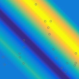
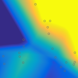
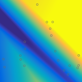
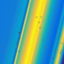
Figure 2: Illustration of learning a low-rank function. (a) Rank-1 data generating function and locations of training samples. (b) Interpolant learned with $L=2$ layers, which does not exhibit rank-1 structure. (c) Interpolant learned with $L=4$ layers, which closely approximates the rank-1 structure of the data-generating function. (d) Result of performing PCA on training features to reduce their dimension to one, followed by learning with $L=2$ layers; standard training methods were unable to find an interpolant along the PCA subspace. This illustration highlights how the addition of linear layers promotes learning single-index models with a central subspace that may differ significantly from the features’ PCA subspace.

3.2 Mixed variation functions

Performing an eigendecomposition on ${\bm{C}}_{f,\rho}$ and discarding small eigenvalues yields an eigenbasis for a low-dimensional subspace that captures directions along which $f$ has large variance. If the columns of a matrix ${\bm{V}}\in\mathbb{R}^{d\times r}$ represent this eigenbasis, then $f({\bm{x}})\approx f({\bm{V}}{\bm{V}}^{\top}{\bm{x}})$ whenever ${\bm{x}},{\bm{V}}{\bm{V}}^{\top}{\bm{x}}\in\mathcal{X}$. More generally $f({\bm{x}})\approx f({\bm{x}}+{\bm{u}})$ for all ${\bm{x}}\in\mathcal{X}$ and all ${\bm{u}}\in\operatorname*{null}({\bm{V}})$ such that ${\bm{x}}+{\bm{u}}\in\mathcal{X}$. Such functions are “approximately low-rank”. In this section, we introduce a notion of mixed variation to formalize and quantify this idea.

Mixed variation function spaces [10] contain functions that are more regular in some directions than in others, and Parhi and Nowak, [29] provides examples of neural networks adapting to a type of mixed variation. In this paper, we define the mixed variation of a function as follows:

Definition 3.3 (Mixed variation).

Given a function $f:\mathcal{X}\rightarrow\mathbb{R}$, we let

$$\sigma_{k}(f;\rho):=\sigma_{k}({\bm{C}}_{f,\rho}^{1/2})$$

for ${\bm{C}}_{f,\rho}$ defined in (9) and for $k=1,\ldots d$. For any $q\in(0,1]$, define the mixed variation of order $q$ of $f$ with respect to $\rho$ as

$$\mathcal{MV}\left(f;\rho,q\right):=\|{\bm{C}}_{f,\rho}^{1/2}\|_{S^{q}}=\left(\sum_{k=1}^{d}\sigma_{k}(f;\rho)^{q}\right)^{1/q}.$$

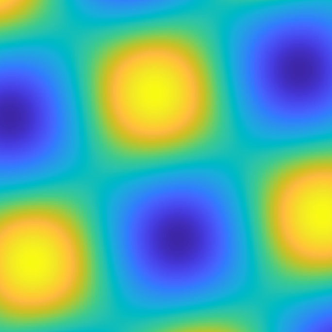
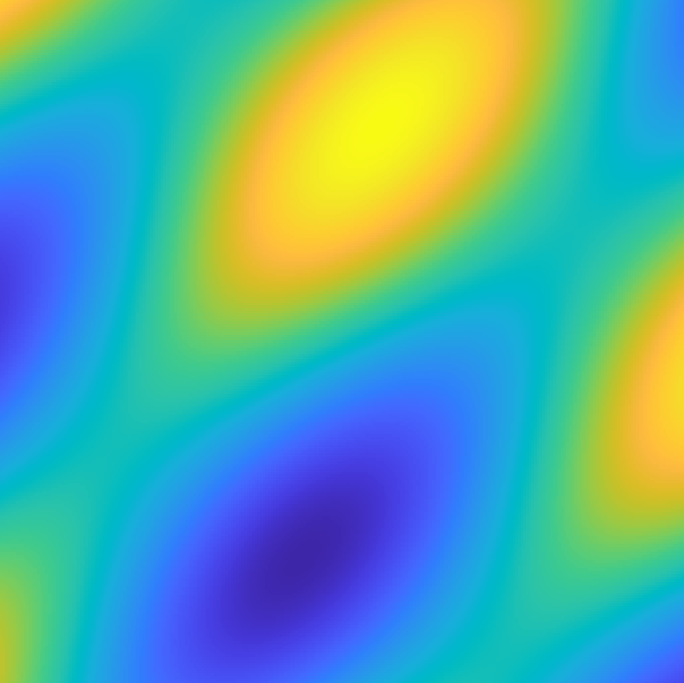
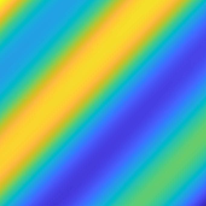
Figure 3: Illustration of four functions in $d=2$ with mixed variation (Definition 3.3) decreasing from left to right. All four functions are rank 2 (Definition 3.2), but the functions on the right with lower mixed variation are closer to being low-rank and vary significantly more in one direction than another.

Note that $\mathcal{MV}\left(f;\rho,q\right)^{q}\rightarrow\operatorname{rank}(f;\rho)$ as $q\rightarrow 0$. Furthermore, as illustrated in Figure 3, functions may be full-rank according to Definition 3.2 but still have low mixed variation when they are “close” to having low rank and vary significantly more in one direction than another, consistent with the notions from [10, 29].

4 Function space perspective

In this section, we show that minimizing the $R_{L}$-cost promotes learning functions that are low-rank or have low mixed variation. We also show that the effective rank of $R_{L}$-cost minimizers must decrease as the number of linear layers $L$ increases, such that asymptotically $R_{L}$-cost minimizing interpolants must be rank one. Additionally, we show that the $R_{2}$-cost of these minimizing interpolants is controlled, so that they will not be too complex or oscillatory. Proofs of results in this section can be found in Appendix C.

4.1 Function rank, mixed variation, and the $R_{L}$-cost

In this section, we establish a relation between the $R_{L}$-cost of a function $f$ and its rank and $R_{2}$-cost, as well as a relation between the $R_{L}$-cost and the mixed variation of a function. Specifically,

Lemma 4.1.

Let $f\in\mathcal{N}_{2}\left(\mathcal{X}\right)$ and $L\geq 2$. Then

$$R_{2}(f)^{2/L}\leq R_{L}(f)\leq\mathrm{rank}(f)^{\frac{L-2}{L}}R_{2}(f)^{2/L}.$$ (11)

The second inequality tells us that a function $f$ with both low rank and small $R_{2}$-cost will have a low $R_{L}$-cost. Consider methods that explicitly learn a single-index or multi-index model to fit training data [43, 40, 6, 20, 13, 12, 5, 23]; such methods, by construction, ensure that $f$ has low rank and has a smooth link function. Thus Lemma 4.1 shows that such methods also control the $R_{L}$-cost of their learned functions; neural networks with $L-1$ linear layers control this cost implicitly. Furthermore, the first inequality guarantees that if we minimize the $R_{L}$-cost during training, then the corresponding $R_{2}$-cost cannot be too high—that is, $R_{L}$ minimizers will not be highly oscillatory in the $R_{2}$ sense.

We further establish that the $R_{L}$-cost is lower bounded by the mixed variation of order $q=2/(L-1)$.

Lemma 4.2.

Let $f\in\mathcal{N}_{2}\left(\mathcal{X}\right)$ and $L\geq 2$. Then

$$\mathcal{MV}\left(f;\rho,\frac{2}{L-1}\right)\leq R_{L}(f)^{L/2}.$$ (12)

This bound is significant because it suggests that when we seek functions with low $R_{L}$-cost to fit training data (e.g., by training a network with $L-1$ linear layers), we ensure that the mixed variation of the learned function will be kept low – in other words, minimizing the $R_{L}$-cost favors functions that are low-rank or approximately low-rank in the mixed variation sense. We establish this formally in the following sections.

4.2 The $R_{L}$-cost favors low-rank functions

Lemma 4.1 and Lemma 4.2 suggest that low-rank functions are favored by the $R_{L}$-cost. In fact, for any pair of functions, adding enough linear layers will eventually favor the lower rank function. This idea is formalized in the following theorem.

Theorem 4.3.

For all $f_{l},f_{h}\in\mathcal{N}_{2}\left(\mathcal{X}\right)$ such that $\operatorname{rank}(f_{l};\rho)<\operatorname{rank}(f_{h};\rho)$, there is a value $L_{0}$ such that $L>L_{0}$ implies $R_{L}(f_{l})<R_{L}(f_{h})$.

Proof.

Let $r_{l}$ and $r_{h}$ denote the ranks of $f_{l}$ and $f_{h}$, respectively. Choose

$$L_{0}:=1+2\frac{\log R_{2}(f_{l})-\frac{1}{2}\log r_{l}-\log\sigma_{r_{h}}(f_{h})}{\log r_{h}-\log r_{l}}.$$

Then $L>L_{0}$ implies

$$r_{l}^{\frac{L-2}{2}}R_{2}(f_{l})<r_{h}^{\frac{L-1}{2}}\sigma_{r_{h}}(f_{h})\leq\mathcal{MV}\left(f_{h};\rho,\tfrac{2}{L-1}\right).$$

By Lemma 4.1 and Lemma 4.2, it follows that $R_{L}(f_{l})<R_{L}(f_{h})$. ∎

Remark 4.4.

Note that Theorem 4.3 holds even when $R_{2}(f_{h})<R_{2}(f_{l})$. That is, there are settings in which two different functions, $f_{l}$ and $f_{h}$, both interpolate a set of training samples, and a shallow two-layer network would select $f_{h}$ over $f_{l}$ because it has the lower $R_{2}$-cost. However, $f_{l}$, the lower-rank function, will be selected over $f_{h}$ if there are sufficiently many linear layers because it will have the smaller $R_{L}$-cost.

4.3 $R_{L}$ minimal functions have low effective rank

Lemma 4.2 has implications for the singular values of trained networks, and thus for their effective rank, i.e., the number of singular values larger than some tolerance $\varepsilon>0$. Given a collection of training data $\mathcal{D}=\{({\bm{x}}_{i},y_{i})\}_{i=1}^{n}$, and a rank cutoff $r$, let $f_{r}=f_{r}(\mathcal{D})$ denote a minimal rank-$r$ $R_{2}$-cost interpolant of the data:

$$f_{r}\in\operatorname*{arg\,min}_{f\in\mathcal{N}_{2}\left(\mathcal{X}\right)}R_{2}(f)~{}~{}\mathrm{s.t.}~{}~{}\operatorname{rank}(f;\rho)\leq r,~{}f({\bm{x}}_{i})=y_{i},\forall i=1,...,n.$$ (13)

and define $M_{r}(\mathcal{D})=R_{2}(f_{r})$, i.e., the minimum $R_{2}$-cost needed to interpolate the data with a rank-$r$ function. We note that if the samples ${\bm{x}}_{i}$ are in general position, a rank-$r$ interpolant will exist. Then we have the following a priori bounds on the singular values of $R_{L}$-cost minimizers:

Theorem 4.5 (Decay of singular values of $R_{L}$-minimal interpolants).

Given training data $\mathcal{D}$, let $\hat{f}_{L}\in\mathcal{N}_{2}\left(\mathcal{X}\right)$ be any interpolant that minimizes the $R_{L}$-cost. Then for all integers $s\geq 1$ and $k\geq 0$ such that $s+k\leq d$,

$$\sigma_{s+k}(\hat{f}_{L};\rho)\leq\frac{M_{s}(\mathcal{D})}{\sqrt{s}}\left(\frac{s}{s+k}\right)^{(L-1)/2}.$$

The presence of $M_{s}(\mathcal{D})$ in the bound in Theorem 4.5 is significant. If the data is generated by a function $f^{*}$ that has rank $r$, one would imagine that $M_{r}(\mathcal{D})$ is much smaller than $M_{s}(\mathcal{D})$ for any $s<r$. In particular, $M_{r}(\mathcal{D})\leq R_{2}(f^{*})$. Thus, the upper bound on the singular values drops greatly between $\sigma_{r}(\hat{f}_{L};\rho)$ and $\sigma_{r+1}(\hat{f}_{L};\rho)$. However, Theorem 4.5 also tells us that $\hat{f}_{L}$ will be approximately a rank one function for very large values of $L$ in the sense that all but one of its singular values will be small.

Corollary 4.6.

For any $k>1$, $\sigma_{k}(\hat{f}_{L};\rho)=O(k^{-L/2})$.

We can extend Theorem 4.5 to regularized empirical risk minimizers and to interpolants that only approximately minimize the $R_{L}$-cost.

Corollary 4.7.

For all constants $C\geq 1$, $\eta>0$ and all integers $s\geq 1$ and $k\geq 0$ such that $s+k\leq d$, if

$$\frac{1}{n}\sum_{i=1}^{n}(y_{i}-\hat{f}({\bm{x}}_{i}))^{2}+\eta R_{L}(\hat{f})\leq C\left(\inf_{f\in\mathcal{N}_{2}\left(\mathcal{X}\right)}\frac{1}{n}\sum_{i=1}^{n}(y_{i}-f({\bm{x}}_{i}))^{2}+\eta R_{L}(f)\right)$$

or if $f({\bm{x}}_{i})=y_{i}$ for all $i=1,\ldots,n$ and $R_{L}(\hat{f})\leq CR_{L}(\hat{f}_{L})$ then

$$\sigma_{s+k}(\hat{f};\rho)\leq\frac{M_{s}(\mathcal{D})}{\sqrt{s}}\left(\frac{s}{s+k}\right)^{(L-1)/2}C^{L/2}.$$

As long as $C\leq 1+\frac{k}{s}$ and $k\geq 1$, this upper bound converges to zero as $L\rightarrow\infty$. Thus, functions that are within a small multiplicative factor of being an $R_{L}$-regularized empirical risk minimizer or $R_{L}$-minimal interpolant will have low effective rank for large $L$.

5 Numerical Experiments

To understand the practical consequences of the theoretical results in the previous section, we performed numerical experiments in which we trained neural networks with and without adding linear layers. All networks in this section are of the form (3) with varying values of $L$. For training details, see Appendix D.

We simulated data where the ground truth is a low-rank function. Specifically, we created a rank-$r$ function $f\in\mathcal{N}_{2}\left([-\frac{1}{2},\frac{1}{2}]^{20}\right)$ by randomly generating ${\bm{a}},{\bm{b}}\in\mathbb{R}^{21}$ and a rank-$r$ matrix ${\bm{W}}\in\mathbb{R}^{21\times 20}$ where we denote the right singular vectors of ${\bm{W}}$ as the columns of ${\bm{V}}\in\mathbb{R}^{20\times r}$. Under this set-up, the function $f({\bm{x}})={\bm{a}}^{\top}[{\bm{W}}{\bm{x}}+{\bm{b}}]_{+}$ is a rank-$r$ function with active subspace $\operatorname{range}({\bm{V}})$.

For $r=1,2$, we generated training pairs $\{({\bm{x}}_{i},f({\bm{x}}_{i}))\}_{i=1}$ where ${\bm{x}}_{i}\sim U([-\frac{1}{2},\frac{1}{2}]^{20})$ and trained randomly initialized neural networks of the form (3) with $L=2$ or $L=4$ with a weight decay parameter of $\lambda=10^{-3}$. We tested the performance of these neural networks on new samples $\{({\bm{x}}_{i},f({\bm{x}}_{i}))\}_{i=1}^{n}$ where either ${\bm{x}}_{i}\sim U([-\frac{1}{2},\frac{1}{2}]^{20})$ to measure generalization performance or ${\bm{x}}_{i}\sim U([-1,1]^{20})$ to measure out-of-distribution performance. We report an estimate of the distance between the active subspace of $f$ and the active subspace of the trained models. Specifically, the distance is measured as the sine of the principal angle between $\operatorname{range}({\bm{V}})$ and the subspace spanned by the top $r$ eigenvectors of an estimate of ${\bm{C}}_{\hat{f},\rho}$ where $\hat{f}$ is the learned network. See Appendix D for details. The results are shown in Table 1, and the singular values of the trained networks are shown in Figure 4. We observe that adding linear layers clearly leads to trained networks with lower effective rank; the singular values $\sigma_{k}$ for larger $k$ of networks with $L=4$ are many orders of magnitude smaller than their counterparts in $L=2$ networks and often follow a sharp dropoff.

Adding linear layers and thereby implicitly selecting a network with low effective rank does not always improve generalization when the number of training samples is too small. In Table 1, observe that when $r=2$ and $n=64$ or $n=128$, the active subspace of the learned network with $L=4$ is far from the active subspace of $f$ and therefore the learned network generalizes poorly. However, after increasing the number of training samples to $n=256$, the learned network properly aligns with $\operatorname{range}({\bm{V}})$. This alignment significantly improves generalization. In fact, the networks that are aligned with $\operatorname{range}({\bm{V}})$ (i.e., $L=4,r=1,n=64$ and $L=4,r=2,n=256$) not only generalize well to new samples from the data-generating distribution, but also to new samples from outside the original distribution.

Plots of training time mean-squared error loss and weight decay can be found in Appendix D. In particular, we observe in Figure 5 that $C_{4}(\theta)$ for the learned network with $L=4,r=2$ and $n=128$ samples is higher than that for $n=256$, suggesting that the model with fewer training samples is converging to a bad local minimizer. Perhaps a specialized initialization could find a minimizer that aligns better with the true active subspace and therefore generalizes.

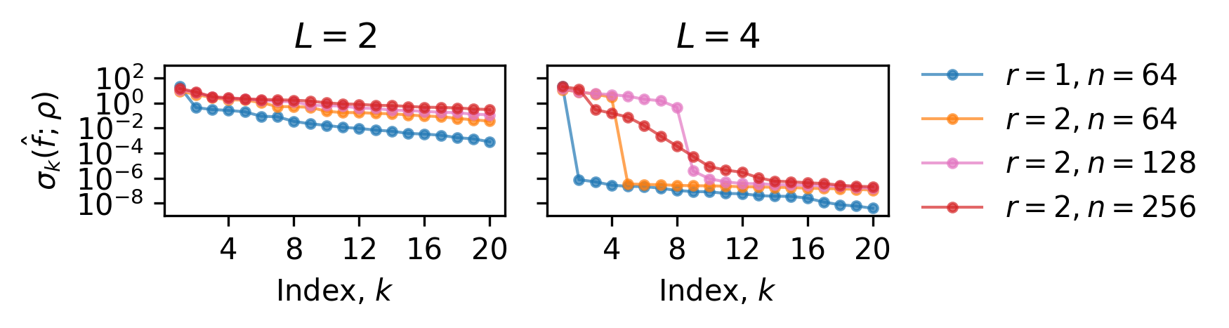
Figure 4: Adding linear layers causes learned networks to have low effective rank. Singular values of trained networks with $L=2$ (left) vs. $L=4$ (right). The singular values of the $L=4$ networks exhibit a sharp dropoff. For example, when $L=4,r=2,n=256$, the first two singular values are approximately 20 and 13, respectively, while the third singular value is approximately 0.3. The dropoffs in singular values of $L=4$ networks are even more extreme for $r=1,n=64;r=2,n=64;$ and $r=2,n=128$. Thus, the effective rank will be smaller for $L=4$ than for $L=2$.

			Train	Generalization	Out of Distribution	Active Subspace
$r$	$n$	$L$	MSE	MSE	MSE	Distance
1	64	2	3.38e-06	1.24e-01	1.09e+00	3.95e-02
		4	8.19e-05	8.86e-04	5.39e-03	2.48e-03
2	64	2	2.69e-07	1.04e+01	4.23e+01	7.59e-01
		4	4.95e-07	1.25e+01	5.02e+01	9.57e-01
2	128	2	7.78e-05	5.97e+00	2.68e+01	4.97e-01
		4	1.74e-05	8.04e+00	3.92e+01	5.88e-01
2	256	2	4.36e-04	4.05e+00	1.87e+01	2.73e-01
		4	9.97e-04	2.35e-02	2.39e-01	1.10e-02

Table 1: With enough data, adding linear layers improves generalization. Results of training neural networks on $n$ samples from a rank-$r$ ground truth function as described in § 5. Train MSE: The mean-squared error of the trained network on training samples $({\bm{x}}_{i},f({\bm{x}}_{i}))$ with ${\bm{x}}_{i}\sim U([-\frac{1}{2},\frac{1}{2}]^{20})$. Generalization MSE: The mean-squared error on new samples with ${\bm{x}}_{i}\sim U([-\frac{1}{2},\frac{1}{2}]^{20})$. Out of Distribution MSE: The mean-squared error on samples with ${\bm{x}}_{i}\sim U([-1,1]^{20})$. Active Subspace Distance: An estimate of the distance between the true active subspace and the active subspace of the learned network.

6 Discussion and Limitations

The representation cost expressions we derive offer new, quantitative insights into the representation costs of multi-layer networks trained using weight decay. Specifically, training a ReLU network with linear layers implicitly seeks a low-dimensional subspace such that a parsimonious two-layer ReLU network can interpolate the projections of the training samples onto the subspace, even when the samples themselves do not lie on a subspace. The representation costs derived imply that ReLU networks with linear layers are able to adapt to latent single- and multi-index models structure underlying the data, giving them the potential to achieve fast rates (depending on the dimension of the latent central subspace) even in high-dimensional settings [20] without designing the network architecture [5] or training [23] to explicitly seek the central subspace. Similarly, prior work has noted that neural networks can achieve faster rates at learning functions that vary more in some directions than in others [29]; this paper provides a formal definition of mixed variation (Definition 3.3) consistent with past usage [10, 28] and characterizes the relationship between mixed variation and neural network representation costs. An additional benefit of this ability to adapt to latent single- and multi-index structure is that trained networks are inherently compressible [23]; given a learned network with parameterization $h_{\theta}^{(L)}$ such that $\theta=({\bm{W}}_{1},{\bm{W}}_{2},...,{\bm{W}}_{L-1},{\bm{a}},{\bm{b}},c)$ and an orthonormal basis for the active subspace of $h_{\theta}^{(L)}$ given as the columns of a matrix ${\bm{V}}$, we have $h_{\theta}^{(L)}({\bm{x}})\approx h_{\theta^{\prime}}^{(3)}({\bm{x}})$ where $\theta^{\prime}=({\bm{U}},{\bm{V}}^{\top},{\bm{a}},{\bm{b}},c)$ for ${\bm{U}}={\bm{W}}_{L-1}\cdots{\bm{W}}_{2}{\bm{W}}_{1}{\bm{V}}$. Additionally, minimizing the $R_{L}$-cost induces sparsity in ${\bm{a}}$, which implies that $h_{\theta}^{(L)}({\bm{x}})$ can be further compressed in width as well as depth.

This paper is an important step towards understanding the representation cost of nonlinear, multi-layer networks. Unlike past work that placed strong assumptions on the data distribution [11] or yields insights only for vector-valued functions [17], our analysis shows that neural networks with linear layers can adapt to latent low-dimensional structure commonly found in single-index or multi-index models without the explicit constraints associated with networks designed explicitly for such models [5, 23]. In addition, we note linear layers can lead to better generalization to new samples. Specifically, § 5 shows that adding linear layers can improve in- and out-of-distribution generalization, and characterizing this behavior theoretically may be an interesting direction for future work.

A key limitation of the current work is that our analysis framework does not extend easily to deep networks with multiple nonlinear layers. The only work of which we are aware addressing this problem places strong assumptions on the distribution of the test and training data or else does not apply to scalar-valued functions. In general, understanding the representation costs of general deep nonlinear networks remains a significant open problem for the community.

7 Acknowledgements

R. Willett gratefully acknowledges the support of AFOSR grant FA9550-18-1-0166 and NSF grant DMS-2023109. G. Ongie was supported by NSF CRII award CCF-2153371. This material is based upon work supported by the National Science Foundation Graduate Research Fellowship under Grant No. DGE:2140001. Any opinions, findings, and conclusions or recommendations expressed in this material are those of the authors and do not necessarily reflect the views of the National Science Foundation.

Appendix A Simplifying the representation cost

In this section we derive simplified expressions for the representation costs $R_{L}$. Proofs of the results in this section are given in Appendix B. Our main result in this section is an explicit description of the $R_{L}$-cost in terms of a penalty $\Phi_{L}$ applied to the inner-layer weight ${\bm{W}}$ matrix and outer-layer weight vector ${\bm{a}}$ of a two-layer network, rather than an $L$-layer network.

First, we prove that the general $R_{L}$-cost can be re-cast as an optimization over two-layer networks, but where the representation cost associated with the inner-layer weight matrix ${\bm{W}}$ changes with $L$:

Lemma A.1.

Suppose $f\in\mathcal{N}_{2}\left(\mathcal{X}\right)$. Then

$$R_{L}(f)=\inf_{\theta\in\Theta_{2}}\tfrac{1}{L}\|{\bm{a}}\|_{2}^{2}+\tfrac{L-1}{L}\|{\bm{W}}\|^{q}_{\mathcal{S}^{q}}~{}~{}\mathrm{s.t.}~{}~{}f=h_{\theta}^{(2)}|_{\mathcal{X}}$$ (14)

where $q:=2/(L-1)$ and $\|{\bm{W}}\|_{\mathcal{S}^{q}}$ is the Schatten-$q$ quasi-norm, i.e., the $\ell^{q}$ quasi-norm of the singular values of ${\bm{W}}$.

Part of the difficulty in interpreting the expression for the $R_{L}$-cost in (14) is that it varies under different sets of parameters realizing the same function. In particular, the loss in (14) may vary under a trivial rescaling of the weights: for any vector $\bm{\lambda}\in\mathbb{R}^{K}$ with positive entries, by the 1-homogeneity of the ReLU activation we have

$${\bm{a}}^{\top}[{\bm{W}}{\bm{x}}+{\bm{b}}]_{+}+c=({\bm{D}}_{\bm{\lambda}}^{-1}{\bm{a}})^{\top}[{\bm{D}}_{\bm{\lambda}}{\bm{W}}{\bm{x}}+{\bm{D}}_{\bm{\lambda}}{\bm{b}}]_{+}+c.$$ (15)

However, the value of the objective in (14) may vary between the two parameter sets realizing the same function. To account for this scaling invariance, we define a new loss function $\Phi_{L}$ by optimizing over all such “diagonal” rescalings of units. Using the AM-GM inequality and a change of variables, one can prove that $\Phi_{L}$ depends only on ${\bm{W}}$ and ${\bm{a}}$ only through the product matrix ${\bm{D}}_{{\bm{a}}}{\bm{W}}$. This leads us to the following result.

Lemma A.2.

For any $f\in\mathcal{N}_{2}\left(\mathcal{X}\right)$, we have

$$R_{L}(f)=\inf_{\theta\in\Theta_{2}}\Phi_{L}({\bm{D}}_{{\bm{a}}}{\bm{W}})~{}~{}\mathrm{s.t.}~{}~{}f=h_{\theta}^{(2)}|_{\mathcal{X}}.$$ (16)

where

$$\Phi_{L}({\bm{D}}_{{\bm{a}}}{\bm{W}})=\inf_{\begin{subarray}{c}\|\bm{\lambda}\|_{2}=1\\ \lambda_{k}>0,\forall k\end{subarray}}\|{\bm{D}}_{\bm{\lambda}}^{-1}{\bm{D}}_{{\bm{a}}}{\bm{W}}\|_{\mathcal{S}^{2/(L-1)}}^{2/L}.$$ (17)

In the case of $L=2$, the infimum in (17) can be computed explicitly as

$$\Phi_{2}({\bm{D}}_{{\bm{a}}}{\bm{W}})=\|{\bm{D}}_{\bm{a}}{\bm{W}}\|_{2,1}=\sum_{k=1}^{K}|a_{k}|\|{\bm{w}}_{k}\|_{2},$$ (18)

which agrees with the expression in (8) after rescaling so that $\|{\bm{w}}_{k}\|_{2}=1$ for all $k$. When $L>2$, there is no such closed form solution. However, (17) still gives some insight into the kinds of functions that have small $R_{L}$-cost. Note that Schatten-$q$ quasi-norms with $0<q\leq 1$ are often used as a surrogate for the rank penalty. Intuitively, the expression for $\Phi_{L}$ reveals that functions with small $R_{L}$ cost have a low-rank inner-layer weight matrix ${\bm{W}}$ and a sparse outer-layer weight vector ${\bm{a}}$. This claim is formally strengthened in the following lemma.

Lemma A.3.

For all $L\geq 2$, we have

$$\Phi_{2}({\bm{D}}_{{\bm{a}}}{\bm{W}})^{2/L}\leq\Phi_{L}({\bm{D}}_{{\bm{a}}}{\bm{W}})\leq\operatorname{rank}({\bm{D}}_{{\bm{a}}}{\bm{W}})^{{(L-2)}/L}\Phi_{2}({\bm{D}}_{{\bm{a}}}{\bm{W}})^{2/L}.$$ (19)

Additionally,

$$\|{\bm{D}}_{\bm{a}}{\bm{W}}\|_{S^{2/L}}^{2/L}\leq\Phi_{L}({\bm{D}}_{{\bm{a}}}{\bm{W}})$$ (20)

Since both the upper bound from (19) and the lower bound from (20) tend toward the rank of ${\bm{D}}_{\bm{a}}{\bm{W}}$ as $L$ goes to infinity, so does $\Phi_{L}$.

Appendix B Proofs of Results in Appendix A

B.1 Proof of Lemma A.1

The result is a direct consequence of the following variational characterization of the Schatten-$q$ quasi-norm for $q=2/\ell$ where $\ell$ is a positive integer:

$$\|{\bm{W}}\|^{2/\ell}_{\mathcal{S}^{2/\ell}}=\min_{{\bm{W}}={\bm{W}}_{1}{\bm{W}}_{2}\cdots{\bm{W}}_{\ell}}\frac{1}{\ell}\left(\|{\bm{W}}_{1}\|_{F}^{2}+\|{\bm{W}}_{2}\|_{F}^{2}+\cdots+\|{\bm{W}}_{\ell}\|_{F}^{2}\right)$$

where the minimization is over all matrices ${\bm{W}}_{1},...,{\bm{W}}_{\ell}$ of compatible dimensions. The case $\ell=2$ is well-known (see, e.g., [34]). The general case for $\ell\geq 3$ is established in [33, Corollary 3].

B.2 Proof of Lemma A.2

Fix any parameterization $f=h_{\theta}^{(2)}|_{\mathcal{X}}$ with $\theta=({\bm{W}},{\bm{a}},{\bm{b}},c)$. Without loss of generality, assume ${\bm{a}}$ has all nonzero entries. By positive homogeneity of the ReLU, for any vector ${\bm{\lambda}}\in\mathbb{R}^{K}$ with positive entries (which we denote by ${\bm{\lambda}}>0$) the rescaled parameters $\theta^{\prime}=({\bm{D}}_{\bm{\lambda}}^{-1}{\bm{W}},{\bm{D}}_{\bm{\lambda}}{\bm{a}},{\bm{D}}_{\bm{\lambda}}^{-1}{\bm{b}},c)$ also satisfy $f=h_{\theta^{\prime}}^{(2)}|_{\mathcal{X}}$. Therefore, by Lemma A.1 we have

$$R_{L}(f) =\inf_{\theta\in\Theta_{2}}\tfrac{1}{L}\|{\bm{a}}\|_{2}^{2}+\tfrac{L-1}{L}\|{\bm{W}}\|^{2/(L-1)}_{\mathcal{S}^{2/(L-1)}}~{}~{}\mathrm{s.t.}~{}~{}f=h_{\theta}^{(2)}|_{\mathcal{X}}$$ (21)

$$=\inf_{\theta\in\Theta_{2}}\inf_{{\bm{\lambda}}>0}\tfrac{1}{L}\|{\bm{D}}_{\bm{\lambda}}{\bm{a}}\|_{2}^{2}+\tfrac{L-1}{L}\|{\bm{D}}_{\bm{\lambda}}^{-1}{\bm{W}}\|^{2/(L-1)}_{\mathcal{S}^{2/(L-1)}}~{}~{}\mathrm{s.t.}~{}~{}f=h_{\theta}^{(2)}|_{\mathcal{X}}.$$ (22)

Additionally, for any fixed $\bm{\lambda}>0$, we may separately minimize over all scalar multiples $c\bm{\lambda}$ where $c>0$, to get

$$\inf_{{\bm{\lambda}}>0}\tfrac{1}{L}\|{\bm{D}}_{\bm{\lambda}}{\bm{a}}\|_{2}^{2}+ \tfrac{L-1}{L}\|{\bm{D}}_{\bm{\lambda}}^{-1}{\bm{W}}\|^{2/(L-1)}_{\mathcal{S}^{2/(L-1)}}$$ (23)

$$=\inf_{\bm{\lambda}>0}\left(\inf_{c>0}c^{2}\tfrac{1}{L}\|{\bm{D}}_{\bm{\lambda}}{\bm{a}}\|_{2}^{2}+c^{-2/(L-1)}\tfrac{L-1}{L}\|{\bm{D}}_{\bm{\lambda}}^{-1}{\bm{W}}\|^{2/(L-1)}_{\mathcal{S}^{2/(L-1)}}\right)$$ (24)

$$=\inf_{\bm{\lambda}>0}\left(\|{\bm{D}}_{\bm{\lambda}}{\bm{a}}\|_{2}\|{\bm{D}}_{\bm{\lambda}}^{-1}{\bm{W}}\|_{\mathcal{S}^{2/(L-1)}}\right)^{2/L}$$ (25)

where the final equality follows by the weighted AM-GM inequality: for all $a,b>0$, it holds that $\tfrac{1}{L}a+\tfrac{L-1}{L}b\geq(ab^{L-1})^{1/L}$, which holds with equality when $a=b$. Here we have $a=(c\|{\bm{D}}_{\bm{\lambda}}{\bm{a}}\|_{2})^{2}$ and $b=\left(c^{-1}\|{\bm{D}}_{\bm{\lambda}}^{-1}{\bm{W}}\|_{\mathcal{S}^{2/(L-1)}}\right)^{2/(L-1)}$, and there exists a $c>0$ for which $a=b$, hence we obtain the lower bound.

Finally, performing the invertible change of variables ${\bm{\lambda}}\mapsto{\bm{\lambda}}^{\prime}$ defined by $\lambda_{k}^{\prime}=|a_{k}|\lambda_{k}$ for all $k=1,...,K$, we have $\|{\bm{D}}_{{\bm{\lambda}}}{\bm{a}}\|_{2}=\|{\bm{D}}_{|{\bm{a}}|}{\bm{\lambda}}\|_{2}=\|{\bm{\lambda}}^{\prime}\|_{2}$ and $\|{\bm{D}}_{\bm{\lambda}}^{-1}{\bm{W}}\|_{{\mathcal{S}}^{q}}=\|{\bm{D}}_{{\bm{\lambda}}^{\prime}}^{-1}{\bm{D}}_{|{\bm{a}}|}{\bm{W}}\|_{{\mathcal{S}}^{q}}=\|{\bm{D}}_{{\bm{\lambda}}^{\prime}}^{-1}{\bm{D}}_{{\bm{a}}}{\bm{W}}\|_{{\mathcal{S}}^{q}}$, and so

$$\inf_{\bm{\lambda}>0}\left(\|{\bm{D}}_{\bm{\lambda}}{\bm{a}}\|_{2}\|{\bm{D}}_{\bm{\lambda}}^{-1}{\bm{W}}\|_{\mathcal{S}^{2/(L-1)}}\right)^{2/L} =\inf_{\bm{\lambda}^{\prime}>0}\left(\|\bm{\lambda}^{\prime}\|_{2}\|{\bm{D}}_{\bm{\lambda}^{\prime}}^{-1}{\bm{D}}_{\bm{a}}{\bm{W}}\|_{\mathcal{S}^{2/(L-1)}}\right)^{2/L}$$ (26)

$$=\inf_{\begin{subarray}{c}\bm{\lambda}^{\prime}>0\\ \|\bm{\lambda}^{\prime}\|_{2}=1\end{subarray}}\|{\bm{D}}_{\bm{\lambda}^{\prime}}^{-1}{\bm{D}}_{\bm{a}}{\bm{W}}\|_{\mathcal{S}^{2/(L-1)}}^{2/L}$$ (27)

where we are able to constrain $\bm{\lambda}^{\prime}$ to be unit norm since $\|\bm{\lambda}^{\prime}\|_{2}\|{\bm{D}}_{\bm{\lambda}^{\prime}}^{-1}{\bm{D}}_{\bm{a}}{\bm{W}}\|_{\mathcal{S}^{2/(L-1)}}$ is invariant to scaling $\bm{\lambda}^{\prime}$ by positive constants.

B.3 Proof of Lemma A.3: Equation 19

Let $q\in(0,1]$ and ${\bm{\sigma}}\in\mathbb{R}^{n}$. It is well known that $\|{\bm{\sigma}}\|_{2}\leq\|{\bm{\sigma}}\|_{q}$. On the other hand, using Jensen’s inequality we see that

$$n^{-\frac{2}{q}}\|{\bm{\sigma}}\|_{q}^{2}=\left(\frac{1}{n}\sum_{i=1}^{n}\sigma_{i}^{q}\right)^{\frac{2}{q}}\leq\frac{1}{n}\left(\sum_{i=1}^{n}\sigma_{i}^{2}\right)=n^{-1}\|{\bm{\sigma}}\|_{2}^{2}.$$ (28)

Thus

$$\|{\bm{\sigma}}\|_{2}\leq\|{\bm{\sigma}}\|_{q}\leq n^{\frac{1}{q}-\frac{1}{2}}\|{\bm{\sigma}}\|_{2}.$$ (29)

When $q=\frac{2}{L-1}$, we have $\frac{1}{q}-\frac{1}{2}=\frac{L-2}{2}$. Extending this result to Schatten norms, for any rank-$r$ matrix ${\bm{X}}$ we have

$$\|{\bm{X}}\|_{F}\leq\|{\bm{X}}\|_{{\mathcal{S}}^{q}}\leq r^{\frac{L-2}{2}}\|{\bm{X}}\|_{F},$$ (30)

using the fact that $\|{\bm{X}}\|_{F}=\|{\bm{X}}\|_{{\mathcal{S}}^{2}}$. Therefore, for all ${\bm{\lambda}}\in\mathbb{R}^{K}_{+}$, ${\bm{a}}\in\mathbb{R}^{K}$, ${\bm{W}}\in\mathbb{R}^{K\times d}$.

$$\|{\bm{D}}_{{\bm{\lambda}}}^{-1}{\bm{D}}_{{\bm{a}}}{\bm{W}}\|_{F}\leq\|{\bm{D}}_{{\bm{\lambda}}}^{-1}{\bm{D}}_{{\bm{a}}}{\bm{W}}\|_{{\mathcal{S}}^{q}}\leq(\operatorname{rank}{{\bm{D}}_{{\bm{a}}}{\bm{W}}})^{\frac{L-2}{2}}\|{\bm{D}}_{{\bm{\lambda}}}^{-1}{\bm{D}}_{{\bm{a}}}{\bm{W}}\|_{F}.$$ (31)

Taking infimums over vectors ${\bm{\lambda}}\in\mathbb{R}^{K}_{+}$ with $\|{\bm{\lambda}}\|=1$ gives

$$\Phi_{2}({\bm{D}}_{{\bm{a}}}{\bm{W}})\leq\Phi_{L}({\bm{D}}_{{\bm{a}}}{\bm{W}})^{L/2}\leq(\operatorname{rank}{{\bm{D}}_{{\bm{a}}}{\bm{W}}})^{\frac{L-2}{2}}\Phi_{2}({\bm{D}}_{{\bm{a}}}{\bm{W}}).$$ (32)

B.4 Proof of Lemma A.3: Equation 20

In [36] it is shown that given matrices ${\bm{A}}\in\mathbb{R}^{d\times K},{\bm{B}}\in\mathbb{R}^{K\times K}$ and a constant $\alpha>0$,

$$\sum_{k=1}^{K}\sigma_{k}^{\alpha}({\bm{A}}{\bm{B}})\geq\sum_{k=1}^{K}\sigma_{k}^{\alpha}({\bm{A}})\sigma_{K-k+1}^{\alpha}({\bm{B}}).$$ (33)

We apply this result to ${\bm{D}}_{{\bm{\lambda}}}^{-1}{\bm{D}}_{\bm{a}}{\bm{W}}$ where ${\bm{\lambda}}>0$:

$$\|{\bm{D}}_{{\bm{\lambda}}}^{-1}{\bm{D}}_{\bm{a}}{\bm{W}}\|_{S^{2/(L-1)}}^{2/(L-1)} =\sum_{k=1}^{K}\sigma_{k}^{2/(L-1)}({\bm{D}}_{{\bm{\lambda}}}^{-1}{\bm{D}}_{\bm{a}}{\bm{W}})$$ (34)

$$=\sum_{k=1}^{K}\sigma_{k}^{2/(L-1)}(({\bm{D}}_{\bm{a}}{\bm{W}})^{\top}{\bm{D}}_{{\bm{\lambda}}}^{-1})$$ (35)

$$\geq\sum_{k=1}^{K}\sigma_{k}^{2/(L-1)}({\bm{D}}_{\bm{a}}{\bm{W}})\sigma_{K-k+1}^{2/(L-1)}({\bm{D}}_{{\bm{\lambda}}}^{-1}).$$ (36)

Observe that $\sigma_{K-k+1}({\bm{D}}_{{\bm{\lambda}}}^{-1})=\sigma_{k}^{-1}({\bm{D}}_{{\bm{\lambda}}})$, so

$$\|{\bm{D}}_{{\bm{\lambda}}}^{-1}{\bm{D}}_{\bm{a}}{\bm{W}}\|_{S^{2/(L-1)}}^{2/(L-1)}\geq\sum_{k=1}^{K}\sigma_{k}^{2/(L-1)}({\bm{D}}_{\bm{a}}{\bm{W}})\sigma_{k}^{-2/(L-1)}({\bm{D}}_{{\bm{\lambda}}}).$$ (37)

Next, we take the infimum over both sides and replace ${\bm{\lambda}}$ with it’s ordered version, ${\bm{\mu}}$:

$$\Phi_{L}({\bm{D}}_{\bm{a}}{\bm{W}})^{L/(L-1)} \geq\inf_{\begin{subarray}{c}\|{\bm{\lambda}}\|_{2}=1,\\ \lambda_{k}>0,\forall k\end{subarray}}\sum_{k=1}^{K}\sigma_{k}^{2/(L-1)}({\bm{D}}_{\bm{a}}{\bm{W}})\sigma_{k}^{-2/(L-1)}({\bm{D}}_{{\bm{\lambda}}}).$$ (38)

$$\geq\min_{\begin{subarray}{c}\|{\bm{\mu}}\|_{2}=1,\\ \mu_{1}\geq\mu_{2}\geq\ldots\geq\mu_{K}\geq 0\end{subarray}}\sum_{k=1}^{K}\sigma_{k}^{2/(L-1)}({\bm{D}}_{\bm{a}}{\bm{W}})\mu_{k}^{-2/(L-1)}$$ (39)

The infimum is replaced with a minimum because we are now minimizing over a compact set. Using Lagrange multipliers, we find that the minimum is attained when

$$\mu_{k}=\begin{cases}\sigma_{k}^{1/L}({\bm{D}}_{\bm{a}}{\bm{W}}){\|{\bm{D}}_{\bm{a}}{\bm{W}}\|_{S^{2/L}}^{-1/L}}&\text{if $k\leq\operatorname{rank}({\bm{D}}_{\bm{a}}{\bm{W}})$}\\ 0&\text{if $k>\operatorname{rank}({\bm{D}}_{\bm{a}}{\bm{W}})$}\end{cases}$$ (40)

and the minimal value is $\|{\bm{D}}_{\bm{a}}{\bm{W}}\|_{S^{2/L}}^{2/(L-1)}$. Therefore,

$$\Phi_{L}({\bm{D}}_{\bm{a}}{\bm{W}})\geq\|{\bm{D}}_{\bm{a}}{\bm{W}}\|_{S^{2/L}}^{2/L}.$$ (41)

Appendix C Proofs of Results in § 4

C.1 Ranks of Neural Networks

Observe that if $f({\bm{x}})=a[{\bm{w}}^{\top}{\bm{x}}+b]_{+}$ then $\nabla f({\bm{x}})=aU({\bm{w}}^{\top}{\bm{x}}+b){\bm{w}}$ where $U$ is the unit step function, and so

$$\nabla f({\bm{x}})\nabla f({\bm{x}})^{\top}=a^{2}U({\bm{w}}^{\top}{\bm{x}}+b){\bm{w}}{\bm{w}}^{\top}.$$ (42)

Likewise, if $f\in\mathcal{N}_{2}\left(\mathcal{X}\right)$ and $f=h_{\theta}^{(2)}|_{\mathcal{X}}$ for some $\theta=({\bm{W}},{\bm{a}},{\bm{b}},c)$, define ${\bm{u}}_{\theta}({\bm{x}})$ as the vector valued function with entries $u_{\theta}^{k}({\bm{x}}):=U({\bm{w}}_{k}^{\top}{\bm{x}}+b_{k})$ for all $k=1,\ldots K$. Then for ${\bm{x}}\in\mathcal{X}$,

$$\nabla f({\bm{x}})\nabla f({\bm{x}})^{\top}=\sum_{k}\sum_{j}a_{k}a_{j}u_{\theta}^{k}({\bm{x}})u_{\theta}^{j}({\bm{x}}){\bm{w}}_{k}{\bm{w}}_{j}^{\top}=({\bm{D}}_{\bm{a}}{\bm{W}})^{\top}{\bm{u}}_{\theta}({\bm{x}}){\bm{u}}_{\theta}({\bm{x}})^{\top}{\bm{D}}_{\bm{a}}{\bm{W}}.$$ (43)

Taking expectations gives

$${\bm{C}}_{f,\rho}=({\bm{D}}_{\bm{a}}{\bm{W}})^{\top}{\bm{U}}_{\theta}{\bm{D}}_{\bm{a}}{\bm{W}}.$$ (44)

where ${\bm{U}}_{\theta}:=\mathbb{E}_{\rho}[{\bm{u}}_{\theta}({\bm{x}}){\bm{u}}_{\theta}({\bm{x}})^{\top}]$ is a matrix of ReLU unit co-activation probabilities under $\rho$. This allows us to connect $\operatorname{rank}(f;\rho)$ to $\operatorname{rank}({\bm{D}}_{\bm{a}}{\bm{W}})$. We begin with the following two lemmas.

Lemma C.1.

Assume $\mathcal{X}$ is convex and has nonempty interior. Let $f\in\mathcal{N}_{2}\left(\mathcal{X}\right)$ and let $\nabla f({\bm{x}})$ denote its weak gradient. Let ${\bm{u}}\in\mathbb{R}^{d}$. If ${\bm{u}}^{\top}\nabla f({\bm{x}})=0$ for almost all ${\bm{x}}\in\mathcal{X}$, then $f({\bm{x}}+{\bm{u}})=f({\bm{x}})$ for all ${\bm{x}}\in\mathcal{X}$ such that ${\bm{x}}+{\bm{u}}\in\mathcal{X}$.

Proof.

If $f\in\mathcal{N}_{2}\left(\mathcal{X}\right)$, then $f$ is a continuous piecewise linear function. Let $\Omega_{1},...,\Omega_{N}\subseteq\mathcal{X}$ denote the disjoint open connected regions over which $f$ is piecewise defined, and let $\chi_{\Omega_{j}}$ denote the indicator function for $\Omega_{j}$. There exist some $\bm{\eta}_{j}\in\mathbb{R}^{d}$ and $c_{j}\in\mathbb{R}$ for $j=1,\ldots N$ such that

$$f({\bm{x}})=\sum_{j=1}^{N}(\bm{\eta}_{j}^{\top}{\bm{x}}+c_{j})\chi_{\Omega_{j}}({\bm{x}})$$

for almost all ${\bm{x}}\in\mathcal{X}$. Observe that $\nabla f({\bm{x}})=\sum_{j}\bm{\eta}_{j}\chi_{\Omega_{j}}({\bm{x}})$ is the weak gradient of $f({\bm{x}})$. Since each $\Omega_{j}$ has positive measure, we see that ${\bm{u}}^{\top}\nabla f({\bm{x}})=0$ for almost all ${\bm{x}}\in\Omega_{j}$ implies ${\bm{u}}^{\top}\bm{\eta}_{j}=0$ for all $j$.

Now assume ${\bm{x}},{\bm{x}}+{\bm{u}}\in\mathcal{X}$. Since $\mathcal{X}$ is convex, for all $t\in[0,1]$ we have ${\bm{x}}+t{\bm{u}}\in\mathcal{X}$. Consider the cardinality of the range of the continuous function $t\mapsto f({\bm{x}}+t{\bm{u}})$. First,

$$\left|\left\{f({\bm{x}}+t{\bm{u}}):t\in[0,1]\right\}\right| \leq\left|\left\{\sum_{j=1}^{N}(\bm{\eta}_{j}^{\top}({\bm{x}}+t{\bm{u}})+c_{j})\chi_{\Omega_{j}}({\bm{x}}+t{\bm{u}}):t\in[0,1]\right\}\right|$$

$$=\left|\left\{\sum_{j=1}^{N}(\bm{\eta}_{j}^{\top}{\bm{x}}+c_{j})\chi_{\Omega_{j}}({\bm{x}}+t{\bm{u}}):t\in[0,1]\right\}\right|$$

because $f$ is the continuous extension of the expression in the right-hand side; on the boundaries between regions, the expression in the right-hand side is equal to zero. Next, observe that

$$\left|\left\{\sum_{j=1}^{N}(\bm{\eta}_{j}^{\top}{\bm{x}}+c_{j})\chi_{\Omega_{j}}({\bm{x}}+t{\bm{u}}):t\in[0,1]\right\}\right|\leq 2^{N}$$

because any term in the sum can take on one of two values. A continuous function with finite range and connected domain must be constant, so $f({\bm{x}})=f({\bm{x}}+t{\bm{u}})$ for all $t\in[0,1]$. In particular, $f({\bm{x}})=f({\bm{x}}+{\bm{u}})$. ∎

Lemma C.2.

Assume $\mathcal{X}$ is convex and has nonempty interior. Suppose

$$f({\bm{x}})=\sum_{k=1}^{K}a_{k}[{\bm{w}}_{k}^{\top}{\bm{x}}+b_{k}]_{+}+{\bm{v}}^{\top}{\bm{x}}+c,~{}~{}\forall{\bm{x}}\in\mathcal{X}$$ (45)

and for $k=1,\ldots K$, the active set boundaries $H_{k}=\{{\bm{x}}:{\bm{w}}_{k}^{\top}{\bm{x}}+b_{k}=0\}$ are distinct and intersect the interior of $\mathcal{X}$. Then ${\bm{v}}\in\operatorname{range}({\bm{C}}_{f,\rho})$ and ${\bm{w}}_{k}\in\operatorname{range}({\bm{C}}_{f,\rho})$ for all $k\in[K]$ such that $a_{k}\neq 0$.

Proof.

It suffices to show that ${\bm{v}},{\bm{w}}_{1},\ldots,{\bm{w}}_{K}\in\operatorname*{null}({\bm{C}}_{f,\rho})^{\perp}$, so fix ${\bm{u}}\in\operatorname*{null}({\bm{C}}_{f,\rho})$. Because $\mathcal{X}$ is convex, Lemma C.1 implies that for all ${\bm{x}}\in\mathcal{X}$ and $\delta\in\mathbb{R}$, $f({\bm{x}}+\delta{\bm{u}})=f({\bm{x}})$ whenever ${\bm{x}}+\delta{\bm{u}}\in\mathcal{X}$. Fix $k\in[K]$, and let $\mathcal{X}^{\mathrm{o}}$ denote the interior of $\mathcal{X}$. Since the active set boundaries intersect $\mathcal{X}^{\mathrm{o}}$ and are distinct, there exists some ${\bm{x}}_{k}\in\mathcal{X}^{\mathrm{o}}$ such that ${\bm{w}}_{k}^{\top}{\bm{x}}_{k}+b_{k}=0$ and ${\bm{w}}_{j}^{\top}{\bm{x}}_{k}+b_{j}\neq 0$ whenever $j\neq k$. For sufficiently small $\varepsilon>0$, we have ${\bm{x}}_{k}\pm\varepsilon{\bm{w}}_{k}\in\mathcal{X}^{\mathrm{o}}$ and $\varepsilon|{\bm{w}}_{j}^{\top}{\bm{w}}_{k}|<|{\bm{w}}_{j}^{\top}{\bm{x}}_{k}+b_{j}|$ whenever $j\neq k$. Observe that ${\bm{w}}_{k}^{\top}({\bm{x}}_{k}+\varepsilon{\bm{w}}_{k})+b_{k}>0$ and ${\bm{w}}_{k}^{\top}({\bm{x}}_{k}-\varepsilon{\bm{w}}_{k})+b_{k}<0$. Additionally, ${\bm{x}}_{k}\pm\varepsilon{\bm{w}}_{k}$ has the same activation pattern as ${\bm{x}}_{k}$ on other units, i.e., $\operatorname{sign}({\bm{w}}_{j}^{\top}({\bm{x}}_{k}\pm\varepsilon{\bm{w}}_{k})+b_{j})=\operatorname{sign}({\bm{w}}_{j}^{\top}{\bm{x}}_{k}+b_{j})$ for $j\neq k$. For sufficiently small $\delta>0$, we have ${\bm{x}}_{k}\pm\varepsilon{\bm{w}}_{k}+\delta{\bm{u}}\in\mathcal{X}^{\mathrm{o}}$, $\delta|{\bm{w}}_{k}^{\top}{\bm{u}}|<\varepsilon\|{\bm{w}}_{k}\|_{2}^{2}$, and $\delta|{\bm{w}}_{j}^{\top}{\bm{u}}|<|{\bm{w}}_{j}^{\top}({\bm{x}}_{k}\pm\varepsilon{\bm{w}}_{k})+b_{j}|$ whenever $j\neq k$. This guarantees that ${\bm{w}}_{k}^{\top}({\bm{x}}_{k}+\varepsilon{\bm{w}}_{k}+\delta{\bm{u}})+b_{k}>0$ and ${\bm{w}}_{k}^{\top}({\bm{x}}_{k}-\varepsilon{\bm{w}}_{k}+\delta{\bm{u}})+b_{k}<0$. Also, ${\bm{x}}_{k}\pm\varepsilon{\bm{w}}_{k}+\delta{\bm{u}}$ has the same activation pattern as ${\bm{x}}_{k}$ and ${\bm{x}}_{k}\pm\varepsilon$ on other units.

Now observe that

$$0 =f({\bm{x}}_{k}-\varepsilon{\bm{w}}_{k}+\delta{\bm{u}})-f({\bm{x}}_{k}-\varepsilon{\bm{w}}_{k})$$ (46)

$$=\sum_{j\in[K]}a_{j}\left([{\bm{w}}_{j}^{\top}({\bm{x}}_{k}-\varepsilon{\bm{w}}_{k}+\delta{\bm{u}})+b_{j}]_{+}-[{\bm{w}}_{j}^{\top}({\bm{x}}_{k}-\varepsilon{\bm{w}}_{k})+b_{j}]_{+}\right)+\delta{\bm{v}}^{\top}{\bm{u}}$$ (47)

$$=\sum_{\begin{subarray}{c}j\in[K]\\ {\bm{w}}_{j}^{\top}{\bm{x}}_{k}+b_{j}>0\end{subarray}}a_{j}\left({\bm{w}}_{j}^{\top}\delta{\bm{u}}\right)+\delta{\bm{v}}^{\top}{\bm{u}}$$ (48)

On the other hand,

$$0 =f({\bm{x}}_{k}+\varepsilon{\bm{w}}_{k}+\delta{\bm{u}})-f({\bm{x}}_{k}+\varepsilon{\bm{w}}_{k})$$

$$=\sum_{j\in[K]}a_{j}\left([{\bm{w}}_{j}^{\top}({\bm{x}}_{k}+\varepsilon{\bm{w}}_{k}+\delta{\bm{u}})+b_{j}]_{+}-[{\bm{w}}_{j}^{\top}({\bm{x}}_{k}+\varepsilon{\bm{w}}_{k})+b_{j}]_{+}\right)+\delta{\bm{v}}^{\top}{\bm{u}}$$

$$=a_{k}\left({\bm{w}}_{k}^{\top}\delta{\bm{u}}\right)+\sum_{\begin{subarray}{c}j\in[K]\\ {\bm{w}}_{j}^{\top}{\bm{x}}_{k}+b_{j}>0\end{subarray}}a_{j}\left({\bm{w}}_{j}^{\top}\delta{\bm{u}}\right)+\delta{\bm{v}}^{\top}{\bm{u}}$$

$$=a_{k}\left({\bm{w}}_{k}^{\top}\delta{\bm{u}}\right)$$

Therefore, ${\bm{w}}_{k}^{\top}{\bm{u}}=0$ and ${\bm{w}}_{k}\in\operatorname*{null}({\bm{C}}_{f,\rho})^{\perp}$ whenever $a_{k}\neq 0$. Since this holds for all $k$, it follows from (48) that ${\bm{v}}\in\operatorname*{null}({\bm{C}}_{f,\rho})^{\perp}$ as well. ∎

We use the previous two lemmas to show that the infimum in (16) can be taken over parameterizations of $f$ with the same rank as $f$.

Lemma C.3.

Assume $\mathcal{X}\subseteq\mathbb{R}^{d}$ is either a bounded convex set with nonempty interior or else $\mathcal{X}=\mathbb{R}^{d}$. Let $f\in\mathcal{N}_{2}\left(\mathcal{X}\right)$. Then

$$R_{L}(f)=\inf_{\theta\in\Theta_{2}}\Phi_{L}({\bm{D}}_{{\bm{a}}}{\bm{W}})~{}~{}\mathrm{s.t.}~{}~{}f=h_{\theta}^{(2)}|_{\mathcal{X}}~{}~{}\mathrm{and}~{}~{}\operatorname{rank}(f;\rho)=\operatorname{rank}({\bm{D}}_{{\bm{a}}}{\bm{W}}).$$ (49)

Proof.

By (44), any parameterization $\theta=({\bm{W}},{\bm{a}},{\bm{b}},c)\in\Theta_{2}$ of $f$ satisfies $\operatorname{rank}(f;\rho)=\operatorname{rank}({\bm{C}}_{f,\rho})\leq\operatorname{rank}({\bm{D}}_{\bm{a}}{\bm{W}})$. It suffices to show that for all $\theta=({\bm{W}},{\bm{a}},{\bm{b}},c)\in\Theta_{2}$ such that $f=h_{\theta}^{(2)}|_{\mathcal{X}}$, there is some $\theta^{\prime}=({\bm{W}}^{\prime},{\bm{a}}^{\prime},{\bm{b}}^{\prime},c^{\prime})\in\Theta_{2}$ such that $f=h_{\theta^{\prime}}^{(2)}|_{\mathcal{X}}$, $\operatorname{rank}(f;\rho)\geq\operatorname{rank}({\bm{D}}_{{\bm{a}}^{\prime}}{\bm{W}}^{\prime})$, and $\Phi_{L}({\bm{D}}_{{\bm{a}}^{\prime}}{\bm{W}}^{\prime})\leq\Phi_{L}({\bm{D}}_{{\bm{a}}}{\bm{W}})$. Fix a parameterization $\theta=({\bm{W}},{\bm{a}},{\bm{b}},c)$ of $f$ with $K$ units so that for all ${\bm{x}}\in\mathcal{X}$

$$f({\bm{x}})=h_{\theta}^{(2)}({\bm{x}})=\sum_{k=1}^{K}a_{k}[{\bm{w}}_{k}^{\top}{\bm{x}}+b_{k}]_{+}+c.$$

Without loss of generality, we may rescale the units and assume that $\|{\bm{w}}_{k}\|_{2}=1$ whenever ${\bm{w}}_{k}\neq 0$.

We first prove the result when $\mathcal{X}$ is bounded. We begin by rewriting $h_{\theta}^{(2)}$ in a way that allows us to apply Lemma C.2. We consider three types of units in $\theta$: units that are active on the entirety of $\mathcal{X}$ (i.e., ${\bm{w}}_{k}^{\top}{\bm{x}}+b_{k}\geq 0\;\forall{\bm{x}}\in\mathcal{X}$), units that are active on none of $\mathcal{X}$ (i.e., ${\bm{w}}_{k}^{\top}{\bm{x}}+b_{k}\leq 0\;\forall{\bm{x}}\in\mathcal{X}$), and units whose active sets intersect the interior of $\mathcal{X}$ (i.e., $H_{k}\cap\mathcal{X}^{\mathrm{o}}\neq\emptyset$). We partition the units whose active sets intersect the interior of $\mathcal{X}$ into equivalence classes based on their active set boundaries and define a set $\Gamma_{1}\subseteq[K]$ with one unit from each class. That is, we say that $j\sim k$ if $({\bm{w}}_{j},b_{j})=\pm({\bm{w}}_{k},b_{k})$ and choose one unit $k$ from each equivalence class with respect to $\sim$ to be in $\Gamma_{1}$. For notational convenience, define $\Gamma_{1}^{k+}:=\{j\in[K]:({\bm{w}}_{k},b_{k})=({\bm{w}}_{j},b_{j})\}$ and $\Gamma_{1}^{k-}:=\{j\in[K]:({\bm{w}}_{k},b_{k})=(-{\bm{w}}_{j},-b_{j})\}$, and let $\Gamma_{2}\subseteq[K]$ denote the set of units that are active on all of $\mathcal{X}$. Given ${\bm{x}}\in\mathcal{X}$, we have

$$f({\bm{x}})=\sum_{k\in\Gamma_{1}}\left(\sum_{j\in\Gamma_{1}^{k+}}a_{j}[{\bm{w}}_{k}^{\top}{\bm{x}}+b_{k}]_{+}+\sum_{j\in\Gamma_{1}^{k-}}a_{j}[-{\bm{w}}_{k}^{\top}{\bm{x}}-b_{k}]_{+}\right)+\sum_{\begin{subarray}{c}k\in\Gamma_{2}\end{subarray}}a_{k}({\bm{w}}_{k}^{\top}{\bm{x}}+b_{k})+c.$$

Using the identity $[-t]_{+}=[t]_{+}-t$, it follows that

$$f({\bm{x}})=\sum_{k\in\Gamma_{1}}\left(\sum_{j\sim k}a_{j}\right)[{\bm{w}}_{k}^{\top}{\bm{x}}+b_{k}]_{+}-\sum_{k\in\Gamma_{1}}\left(\sum_{j\in\Gamma_{1}^{k-}}a_{j}\right)({\bm{w}}_{k}^{\top}{\bm{x}}+b_{k})+\sum_{\begin{subarray}{c}k\in\Gamma_{2}\end{subarray}}a_{k}({\bm{w}}_{k}^{\top}{\bm{x}}+b_{k})+c.$$

Lemma C.2 applies to this form and implies that ${\bm{w}}_{k}\in\operatorname{range}({\bm{C}}_{f,\rho})$ whenever $k\in\Gamma_{1}$ and $\sum_{j\sim k}a_{j}\neq 0.$ Lemma C.2 also implies that

$$\sum_{k\in\Gamma_{2}}a_{k}{\bm{w}}_{k}-\sum_{k\in\Gamma_{1}}\left(\sum_{j\in\Gamma_{1}^{k-}}a_{j}\right){\bm{w}}_{k}\in\operatorname{range}({\bm{C}}_{f,\rho}).$$

For convenience, let $\Gamma_{1}^{\prime}:=\{k\in\Gamma_{1}:\sum_{j\sim k}a_{j}\neq 0\}$ and $\Gamma_{1}^{\prime\prime}:=\{k\in\Gamma_{1}:\sum_{j\sim k}a_{j}=0\}$. Since ${\bm{w}}_{k}\in\operatorname{range}({\bm{C}}_{f,\rho})$ for all $k\in\Gamma_{1}^{\prime}$, we must have

$$\sum_{k\in\Gamma_{2}}a_{k}{\bm{w}}_{k}-\sum_{k\in\Gamma_{1}^{\prime\prime}}\left(\sum_{j\in\Gamma_{1}^{k-}}a_{j}\right){\bm{w}}_{k}\in\operatorname{range}({\bm{C}}_{f,\rho}).$$ (50)

To create $\theta^{\prime}=({\bm{W}}^{\prime},{\bm{a}}^{\prime},{\bm{b}}^{\prime},c^{\prime})$, we keep only the units from $\theta$ that are ever active on $\mathcal{X}$, project all the weights onto $\operatorname{range}({\bm{C}}_{f,\rho})$, and shift units corresponding to $\Gamma_{2}$ and $\Gamma_{1}^{\prime\prime}$ so that they are active on all of $\mathcal{X}$. More formally, let ${\bm{P}}\in\mathbb{R}^{d\times d}$ be the orthogonal projection onto the range of ${\bm{C}}_{f,\rho}$. Since $\mathcal{X}$ is bounded, there is some $B>0$ such that $\|{\bm{x}}\|_{2}\leq B$ for all ${\bm{x}}\in\mathcal{X}$. For any ${\bm{x}}\in\mathcal{X}$,

$$f({\bm{x}}) =\sum_{k\in\Gamma_{1}^{\prime}}\left(\sum_{j\sim k}a_{j}\right)[{\bm{w}}_{k}^{\top}{\bm{x}}+b_{k}]_{+}-\sum_{k\in\Gamma_{1}^{\prime}}\left(\sum_{j\in\Gamma_{1}^{k-}}a_{j}\right)({\bm{w}}_{k}^{\top}{\bm{x}}+b_{k})$$ (51)

$$\quad+\sum_{k\in\Gamma_{1}^{\prime\prime}}\left(\sum_{j\sim k}a_{j}\right)[{\bm{w}}_{k}^{\top}{\bm{x}}+b_{k}]_{+}-\sum_{k\in\Gamma_{1}^{\prime\prime}}\left(\sum_{j\in\Gamma_{1}^{k-}}a_{j}\right)({\bm{w}}_{k}^{\top}{\bm{x}}+b_{k})$$ (52)

$$\quad+\sum_{\begin{subarray}{c}k\in\Gamma_{2}\end{subarray}}a_{k}({\bm{w}}_{k}^{\top}{\bm{x}}+b_{k})+c$$ (53)

$$=\sum_{k\in\Gamma_{1}^{\prime}}\sum_{j\sim k}a_{j}[{\bm{w}}_{j}^{\top}{\bm{x}}+b_{j}]_{+}-\sum_{k\in\Gamma_{1}^{\prime\prime}}\left(\sum_{j\in\Gamma_{1}^{k-}}a_{j}\right)({\bm{w}}_{k}^{\top}{\bm{x}}+b_{k})+\sum_{\begin{subarray}{c}k\in\Gamma_{2}\end{subarray}}a_{k}({\bm{w}}_{k}^{\top}{\bm{x}}+b_{k})+c$$ (54)

because the two terms in (51) can be combined via the identity $[-t]_{+}=[t]_{+}-t$, and the first term in (52) is equal to zero. From (50) and the fact that ${\bm{w}}_{j}\in\operatorname{range}({\bm{C}}_{f,\rho})$ whenever $j\sim k$ and $k\in\Gamma_{1}^{\prime}$, it follows that

$$f({\bm{x}}) =\sum_{k\in\Gamma_{1}^{\prime}}\sum_{j\sim k}a_{j}[{\bm{w}}_{j}^{\top}{\bm{P}}{\bm{x}}+b_{j}]_{+}-\sum_{k\in\Gamma_{1}^{\prime\prime}}\left(\sum_{j\in\Gamma_{1}^{k-}}a_{j}\right)({\bm{w}}_{k}^{\top}{\bm{P}}{\bm{x}}+b_{k})+\sum_{\begin{subarray}{c}k\in\Gamma_{2}\end{subarray}}a_{k}({\bm{w}}_{k}^{\top}{\bm{P}}{\bm{x}}+b_{k})+c$$ (55)

$$=\sum_{k\in\Gamma_{1}^{\prime}}\sum_{j\sim k}a_{j}[{\bm{w}}_{j}^{\top}{\bm{P}}{\bm{x}}+b_{j}]_{+}+\sum_{k\in\Gamma_{1}^{\prime\prime}}\sum_{j\in\Gamma_{1}^{k-}}a_{j}({\bm{w}}_{j}^{\top}{\bm{P}}{\bm{x}}+b_{j})+\sum_{\begin{subarray}{c}k\in\Gamma_{2}\end{subarray}}a_{k}({\bm{w}}_{k}^{\top}{\bm{P}}{\bm{x}}+b_{k})+c$$ (56)

We now shift the units in the second two terms of (56) so that they are active on all of $\mathcal{X}$. Observe that ${\bm{w}}_{k}{\bm{P}}{\bm{x}}+B\geq-\|{\bm{w}}_{k}\|_{2}\|{\bm{x}}\|_{2}+B\geq 0$. Thus,

$$f({\bm{x}}) =\sum_{k\in\Gamma_{1}^{\prime}}\sum_{j\sim k}a_{j}[{\bm{w}}_{j}^{\top}{\bm{P}}{\bm{x}}+b_{j}]_{+}+\sum_{k\in\Gamma_{1}^{\prime\prime}}\sum_{j\in\Gamma_{1}^{k-}}a_{j}[{\bm{w}}_{j}^{\top}{\bm{P}}{\bm{x}}+B]_{+}+\sum_{\begin{subarray}{c}k\in\Gamma_{2}\end{subarray}}a_{k}[{\bm{w}}_{k}^{\top}{\bm{P}}{\bm{x}}+B]_{+}$$ (57)

$$\quad+c+\sum_{\begin{subarray}{c}k\in\Gamma_{2}\end{subarray}}a_{k}(b_{k}-B)+\sum_{k\in\Gamma_{1}^{\prime\prime}}\sum_{j\in\Gamma_{1}^{k-}}a_{j}(b_{j}-B).$$ (58)

Choose $\theta^{\prime}$ to be this new parameterization of $f$. The matrix ${\bm{D}}_{{\bm{a}}^{\prime}}{\bm{W}}^{\prime}$ corresponds to a subset of the rows of ${\bm{D}}_{{\bm{a}}}{\bm{W}}{\bm{P}}$, so we must have $\operatorname{rank}({\bm{D}}_{{\bm{a}}^{\prime}}{\bm{W}}^{\prime})\leq\operatorname{rank}({\bm{P}})=\operatorname{rank}(f;\rho)$. By Lemma 2 in [36] it follows that

$$\Phi_{L}({\bm{D}}_{{\bm{a}}^{\prime}}{\bm{W}}^{\prime}) =\inf_{\begin{subarray}{c}\|\bm{\lambda}\|_{2}=1\\ \lambda_{k}>0,\forall k\end{subarray}}\|{\bm{D}}_{\bm{\lambda}}^{-1}{\bm{D}}_{{\bm{a}}^{\prime}}{\bm{W}}^{\prime}\|_{\mathcal{S}^{2/(L-1)}}^{2/L}$$

$$\leq\inf_{\begin{subarray}{c}\|\bm{\lambda}\|_{2}=1\\ \lambda_{k}>0,\forall k\end{subarray}}\|{\bm{D}}_{\bm{\lambda}}^{-1}{\bm{D}}_{{\bm{a}}}{\bm{W}}{\bm{P}}\|_{\mathcal{S}^{2/(L-1)}}^{2/L}$$

$$\leq\inf_{\begin{subarray}{c}\|\bm{\lambda}\|_{2}=1\\ \lambda_{k}>0,\forall k\end{subarray}}\|{\bm{D}}_{\bm{\lambda}}^{-1}{\bm{D}}_{{\bm{a}}}{\bm{W}}\|_{\mathcal{S}^{2/(L-1)}}^{2/L}$$

$$=\Phi_{L}({\bm{D}}_{{\bm{a}}}{\bm{W}})$$

Finally, if $\mathcal{X}=\mathbb{R}^{d}$, then choosing $\theta^{\prime}=({\bm{W}}{\bm{P}},{\bm{a}},{\bm{b}},c)$ suffices; for any ${\bm{x}}\in\mathbb{R}^{d}$, we have

$$h_{\theta^{\prime}}^{(2)}({\bm{x}})=h_{\theta}^{(2)}({\bm{P}}{\bm{x}})=f({\bm{P}}{\bm{x}})=f({\bm{x}})$$ (59)

since ${\bm{x}}={\bm{P}}{\bm{x}}+(I-{\bm{P}}){\bm{x}}$ and $(I-{\bm{P}}){\bm{x}}\in\operatorname*{null}({\bm{C}}_{f,\rho})$. ∎

C.2 Proof of Lemma 4.1

Proof.

Let $f\in\mathcal{N}_{2}\left(\mathcal{X}\right)$ and $L\geq 2$. By Lemma A.2 and Lemma A.3,

$$R_{2}(f)^{2/L}\leq R_{L}(f)\leq\inf_{\theta:f=h_{\theta}^{(2)}|_{\mathcal{X}}}\operatorname{rank}({\bm{D}}_{{\bm{a}}}{\bm{W}})^{(L-2)/L}\Phi_{2}({\bm{D}}_{{\bm{a}}}{\bm{W}})^{2/L}$$

By Lemma C.3,

$$\operatorname{rank}(f;\rho)^{(L-2)/L}R_{2}(f)^{2/L} =\operatorname{rank}(f;\rho)^{(L-2)/L}\inf_{\begin{subarray}{c}\theta:f=h_{\theta}^{(2)}|_{\mathcal{X}}\\ \operatorname{rank}(f;\rho)=\operatorname{rank}({\bm{D}}_{{\bm{a}}}{\bm{W}})\end{subarray}}\Phi_{2}({\bm{D}}_{{\bm{a}}}{\bm{W}})^{2/L}$$ (60)

$$=\inf_{\begin{subarray}{c}\theta:f=h_{\theta}^{(2)}|_{\mathcal{X}}\\ \operatorname{rank}(f;\rho)=\operatorname{rank}({\bm{D}}_{{\bm{a}}}{\bm{W}})\end{subarray}}\operatorname{rank}({\bm{D}}_{{\bm{a}}}{\bm{W}})^{(L-2)/L}\Phi_{2}({\bm{D}}_{{\bm{a}}}{\bm{W}})^{2/L}$$ (61)

$$\geq\inf_{\theta:f=h_{\theta}^{(2)}|_{\mathcal{X}}}\operatorname{rank}({\bm{D}}_{{\bm{a}}}{\bm{W}})^{(L-2)/L}\Phi_{2}({\bm{D}}_{{\bm{a}}}{\bm{W}})^{2/L}$$ (62)

Therefore

$$R_{2}(f)^{2/L}\leq R_{L}(f)\leq\operatorname{rank}(f;\rho)^{(L-2)/L}R_{2}(f)^{2/L}.$$ (63)

as claimed. ∎

C.3 Proof of Lemma 4.2

Proof.

Fix $f\in\mathcal{N}_{2}\left(\mathcal{X}\right)$ and assume $f=h_{\theta}^{(2)}|_{\mathcal{X}}$ for some $\theta=({\bm{W}},{\bm{a}},{\bm{b}},c)$. Let ${\bm{U}}_{\theta}^{1/2}$ be a matrix square root of ${\bm{U}}_{\theta}$. By (44), a nonsymetric square root of ${\bm{C}}_{f,\rho}$ is given by ${\bm{C}}_{f,\rho}^{1/2}={\bm{U}}_{\theta}^{1/2}{\bm{D}}_{\bm{a}}{\bm{W}}$, and so we have $\mathcal{MV}\left(f;\rho,q\right)=\|{\bm{U}}_{\theta}^{1/2}{\bm{D}}_{\bm{a}}{\bm{W}}\|_{S^{q}}$.

Now fix any vector $\bm{\lambda}>0$ such that $\|\bm{\lambda}\|_{2}=1$. Then we have

$$\mathcal{MV}\left(f;\rho,q\right) =\|{\bm{U}}_{\theta}^{1/2}{\bm{D}}_{\bm{a}}{\bm{W}}\|_{S^{q}}$$ (64)

$$=\|{\bm{U}}_{\theta}^{1/2}{\bm{D}}_{\bm{\lambda}}{\bm{D}}_{\bm{\lambda}}^{-1}{\bm{D}}_{\bm{a}}{\bm{W}}\|_{S^{q}}$$ (65)

$$\leq\|{\bm{U}}_{\theta}^{1/2}{\bm{D}}_{\bm{\lambda}}\|_{op}\|{\bm{D}}_{\bm{\lambda}}^{-1}{\bm{D}}_{\bm{a}}{\bm{W}}\|_{S^{q}}.$$ (66)

Observe that ${\bm{U}}_{\theta}^{1/2}{\bm{D}}_{\bm{\lambda}}$ is a matrix square-root of ${\bm{D}}_{\bm{\lambda}}{\bm{U}}_{\theta}{\bm{D}}_{\bm{\lambda}}$, and so

$$\|{\bm{U}}_{\theta}^{1/2}{\bm{D}}_{\bm{\lambda}}\|_{op} =\|{\bm{D}}_{\bm{\lambda}}{\bm{U}}_{\theta}{\bm{D}}_{\bm{\lambda}}\|_{op}^{1/2},$$ (67)

Furthermore,

$$\|{\bm{D}}_{\bm{\lambda}}{\bm{U}}_{\theta}{\bm{D}}_{\bm{\lambda}}\|_{op} =\max_{\|{\bm{v}}\|_{2}=1}{\bm{v}}^{\top}{\bm{D}}_{\bm{\lambda}}{\bm{U}}_{\theta}{\bm{D}}_{\bm{\lambda}}{\bm{v}}$$ (68)

$$=\max_{\|{\bm{v}}\|_{2}=1}{\bm{v}}^{\top}{\bm{D}}_{\bm{\lambda}}\mathbb{E}_{\rho}[{\bm{u}}_{\theta}({\bm{x}}){\bm{u}}_{\theta}({\bm{x}})^{\top}]{\bm{D}}_{\bm{\lambda}}{\bm{v}}$$ (69)

$$=\max_{\|{\bm{v}}\|_{2}=1}\mathbb{E}_{\rho}[|{\bm{v}}^{\top}{\bm{D}}_{\bm{\lambda}}{\bm{u}}_{\theta}({\bm{x}})|^{2}]$$ (70)

$$\leq\max_{\|{\bm{v}}\|_{2}=1}\mathbb{E}_{\rho}[\|{\bm{v}}\|_{2}^{2}\|{\bm{D}}_{\bm{\lambda}}{\bm{u}}_{\theta}({\bm{x}})\|_{2}^{2}]$$ (71)

$$=\mathbb{E}_{\rho}[\|{\bm{D}}_{\bm{\lambda}}{\bm{u}}_{\theta}({\bm{x}})\|_{2}^{2}]$$ (72)

$$\leq\mathbb{E}_{\rho}[1]=1$$ (73)

where in the last inequality we used the fact that $\|{\bm{D}}_{\bm{\lambda}}{\bm{u}}_{\theta}({\bm{x}})\|_{2}\leq\|\bm{\lambda}\|_{2}=1$ for all ${\bm{x}}\in\mathbb{R}^{d}$ since ${\bm{u}}_{\theta}({\bm{x}})\in\{0,1\}^{K}$. Therefore, we have shown $\|{\bm{D}}_{\bm{\lambda}}{\bm{U}}_{\theta}{\bm{D}}_{\bm{\lambda}}\|_{op}\leq 1$ which implies $\|{\bm{U}}_{\theta}^{1/2}{\bm{D}}_{\bm{\lambda}}\|_{op}\leq 1$. Combining this fact with the inequality above, we see that

$$\mathcal{MV}\left(f;\rho,q\right)\leq\|{\bm{D}}_{\bm{\lambda}}^{-1}{\bm{D}}_{\bm{a}}{\bm{W}}\|_{S^{q}}.$$

Since this inequality is independent of the choice of $\bm{\lambda}$, we have

$$\mathcal{MV}\left(f;\rho,q\right)\leq\inf_{\begin{subarray}{c}\|\bm{\lambda}\|_{2}=1\\ \bm{\lambda}>0\end{subarray}}\|{\bm{D}}_{\bm{\lambda}}^{-1}{\bm{D}}_{\bm{a}}{\bm{W}}\|_{S^{q}}=\Phi_{L}({\bm{D}}_{\bm{a}}{\bm{W}})^{L/2}$$

Finally, since the above inequality holds independent of the choice of parameters $\theta$ realizing $f$, we have

$$\mathcal{MV}\left(f;\rho,q\right)\leq\inf_{\theta:f=h_{\theta}^{(2)}|_{\mathcal{X}}}\Phi_{L}({\bm{D}}_{\bm{a}}{\bm{W}})^{L/2}=R_{L}(f)^{L/2},$$

as claimed.

∎

C.4 Proof of Theorem 4.5

Proof.

For $1\leq s\leq d$ we have

$$R_{L}(\hat{f}_{L})^{L/2} \leq\inf_{f\in\mathcal{N}_{2}\left(\mathcal{X}\right)}R_{L}(f)^{L/2}~{}~{}\mathrm{s.t.}~{}~{}\operatorname{rank}(f;\rho)\leq s,~{}f({\bm{x}}_{i})=y_{i},\forall i=1,...,n$$

$$\leq s^{(L-2)/2}\inf_{f\in\mathcal{N}_{2}\left(\mathcal{X}\right)}R_{2}(f)~{}~{}\mathrm{s.t.}~{}~{}\operatorname{rank}(f;\rho)\leq s,~{}f({\bm{x}}_{i})=y_{i},\forall i=1,...,n$$

$$=s^{(L-2)/2}M_{s}(\mathcal{D})$$

where the second line follows from Lemma 4.1. On the other hand, Lemma 4.2 tells us that

$$R_{L}(\hat{f}_{L})^{L/2}\geq\mathcal{MV}\left(f;\rho,\tfrac{2}{L-1}\right)\geq(s+k)^{(L-1)/2}\sigma_{s+k}(\hat{f}_{L};\rho).$$

Rearranging these inequalities gives the desired result. ∎

C.5 Proof of Corollary 4.6

Proof.

Applying Theorem 4.5 with $s=1$ gives

$$\sigma_{k}(\hat{f}_{L};\rho)\leq M_{1}(\mathcal{D})\left(\frac{1}{k}\right)^{(L-1)/2}=O(k^{-L/2})$$

for all $k\geq 1$. ∎

C.6 Proof of Corollary 4.7

Proof.

We prove the result under the assumption that

$$\frac{1}{n}\sum_{i=1}^{n}(y_{i}-\hat{f}({\bm{x}}_{i}))^{2}+\eta R_{L}(\hat{f})\leq C\left(\inf_{f\in\mathcal{N}_{2}\left(\mathcal{X}\right)}\frac{1}{n}\sum_{i=1}^{n}(y_{i}-f({\bm{x}}_{i}))^{2}+\eta R_{L}(f)\right).$$

The proof when $R_{L}(\hat{f})\leq CR_{L}(\hat{f}_{L})$ is similar. Observe that

$$\eta R_{L}(\hat{f}) \leq\frac{1}{n}\sum_{i=1}^{n}(y_{i}-\hat{f}({\bm{x}}_{i}))^{2}+\eta R_{L}(\hat{f})$$

$$\leq C\left(\inf_{f\in\mathcal{N}_{2}\left(\mathcal{X}\right)}\frac{1}{n}\sum_{i=1}^{n}(y_{i}-f({\bm{x}}_{i}))^{2}+\eta R_{L}(f)\right)$$

$$\leq C\left(\frac{1}{n}\sum_{i=1}^{n}(y_{i}-\hat{f}_{L}({\bm{x}}_{i}))^{2}+\eta R_{L}(\hat{f}_{L})\right)$$

$$=C\eta R_{L}(\hat{f}_{L})$$

$$\leq C\eta s^{(L-2)/L}M_{s}(\mathcal{D})^{2/L}$$

where the last line is as in the proof of Theorem 4.5. By Lemma 4.2

$$R_{L}(\hat{f})^{L/2}\geq\mathcal{MV}\left(\hat{f};\rho,\tfrac{2}{L-1}\right)\geq(s+k)^{(L-1)/2}\sigma_{s+k}(\hat{f};\rho).$$

Thus

$$(s+k)^{(L-1)/2}\sigma_{s+k}(\hat{f};\rho)\leq R_{L}(\hat{f})^{L/2}\leq C^{L/2}s^{(L-2)/2}M_{s}(\mathcal{D}).$$

∎

Appendix D Details of Numerical Experiments

For each value of $(r,n)\in\{(1,64),(2,64),(2,128),(2,256)\}$, we generated $n$ training samples as described in § 5 where

• ${\bm{V}}\;(20\times r)$ is the first $r$ columns of a random orthogonal matrix

• ${\bm{U}}\;(21\times r)$ is the first $r$ columns of a random orthogonal matrix

• $\mathbf{\Sigma}\;(r\times r)$ is a diagonal matrix with entries drawn from $U([0,100])$

• ${\bm{W}}={\bm{U}}\mathbf{\Sigma}{\bm{V}}^{\top}\;(21\times 20)$

• ${\bm{a}},{\bm{b}}\;(21\times 1)$ are vectors with entries drawn from the standard normal distribution.

Then for each $L\in\{2,4\}$, we trained a model of the form (3) starting from PyTorch’s default initialization using Adam with a learning rate of $10^{-4}$ for 30,000 epochs with a weight decay of $\lambda$ followed by $100$ epochs with a learning rate of $10^{-5}$ and no weight decay. The purpose of this final training period was to ensure near-interpolation of the trained networks. For $(r,n,L)$, we tuned $\lambda$ using a small grid search of $\lambda\in\{10^{-3},10^{-4},10^{-5}\}$ by choosing the value of $\lambda$ that gave the best mean-squared error on a validation set of size 1024; $\lambda=10^{-3}$ was always the best parameter. Plots of the mean-squared error on the training set and the weight decay term (the sum of the squares of the regularized, i.e., non-bias parameters) of the models with $\lambda=10^{-3}$ during training time are shown in Figure 5. Training all 24 models took approximately one hour total on a T4 GPU via Google Colab.

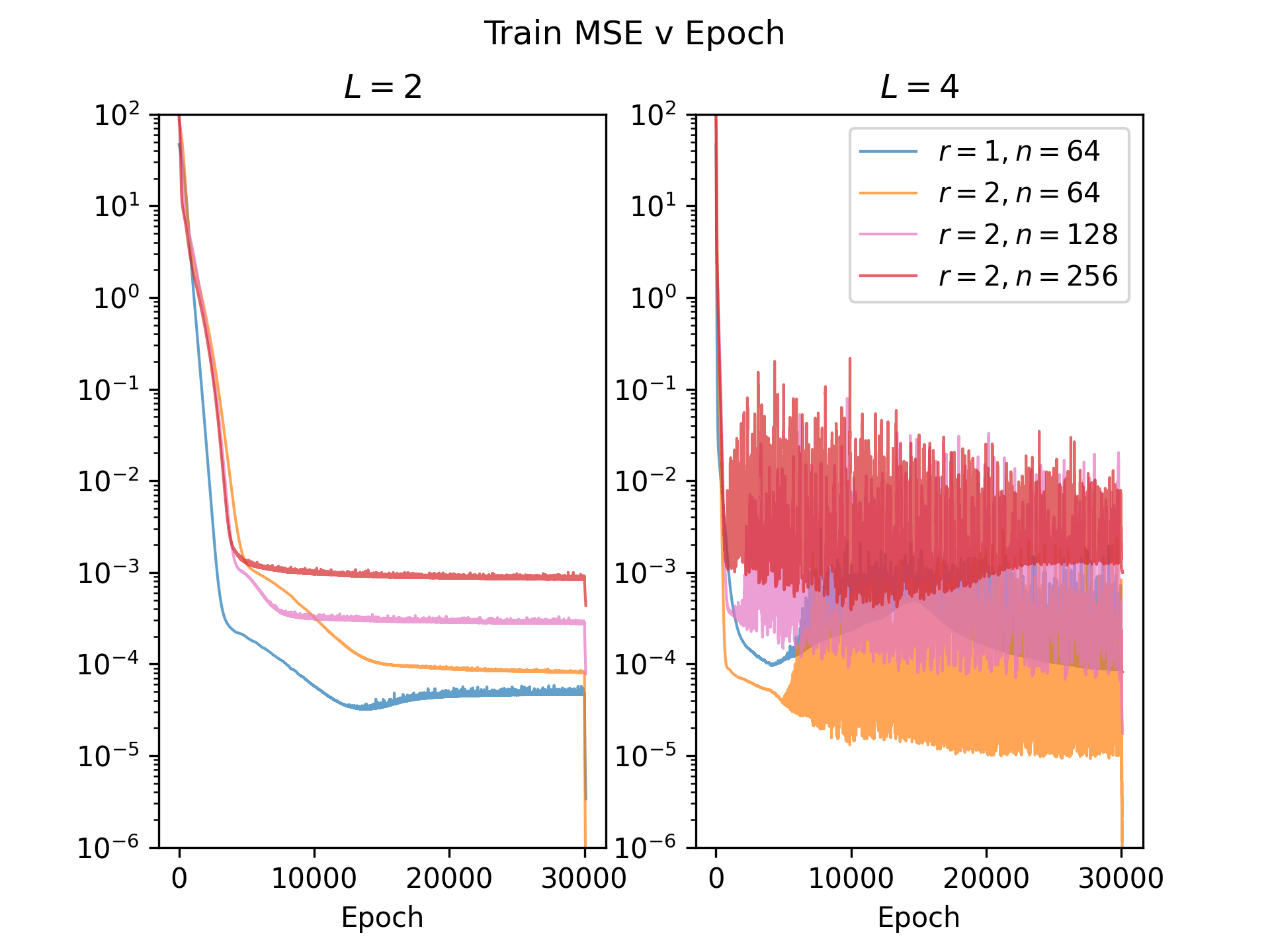
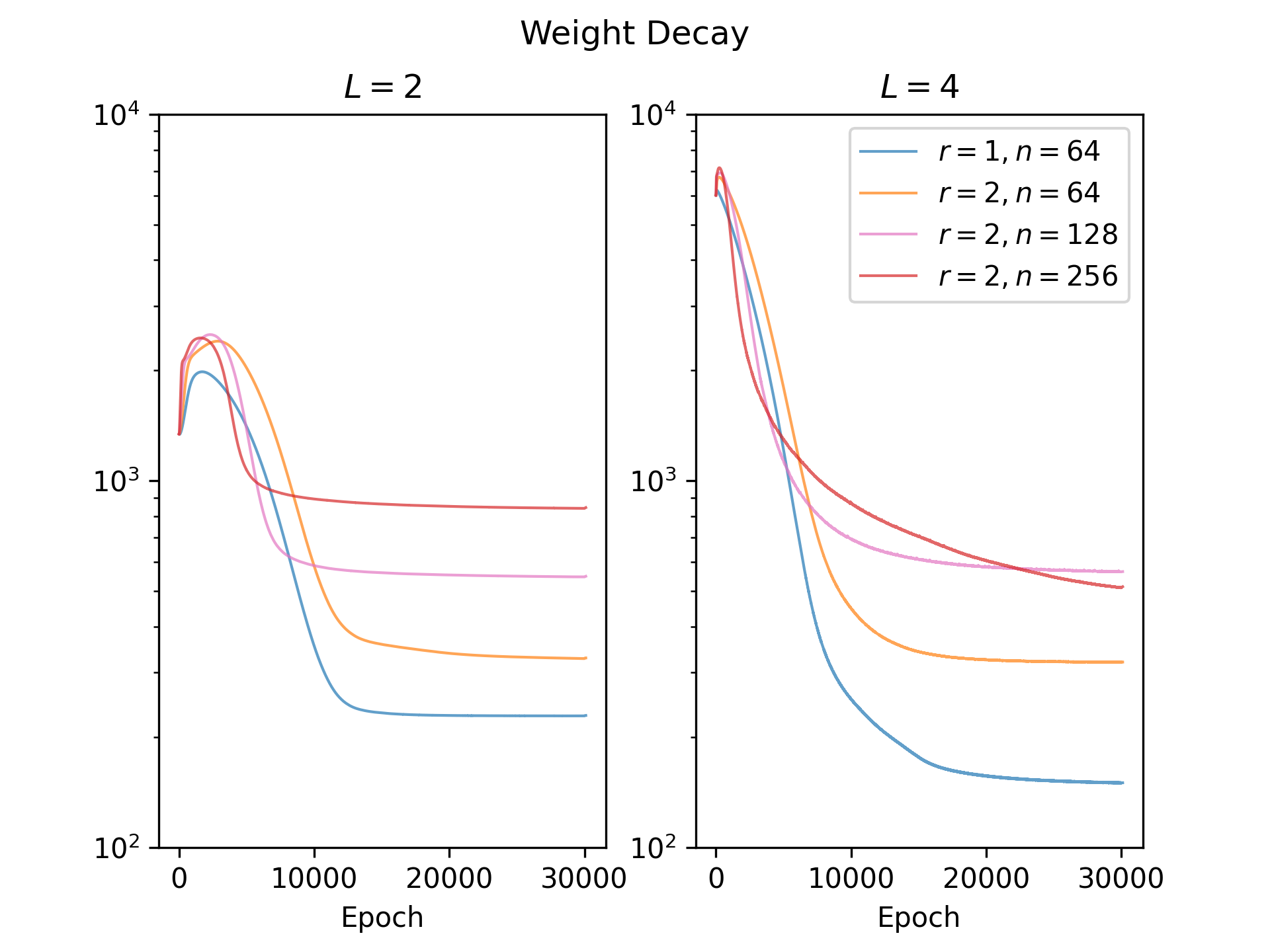
Figure 5: Training time (a) mean-squared error loss on training samples and (b) weight decay term. All models shown here are trained with a weight decay parameter of $\lambda=10^{-3}$, and demonstrate good convergence to (local) minimizers. Notice that the weight decay term for the model with $L=4,r=2,n=256$ is smaller than that for $L=4,r=2,n=128$. This suggests that the model with $L=4,r=2,n=256$ is converging to a bad local minimizer.

We then generated 2048 new test samples with ${\bm{x}}_{i}\sim U([-\frac{1}{2},\frac{1}{2}])$ for $r=1,2$ and computed the mean-squared error on these test samples; this value is reported in Table 1 as the generalization error. Next, we generated 2048 new test samples with ${\bm{x}}_{i}\sim U([-1,1])$ for $r=1,2$, as reported in Table 1 as the out-of-distribution error.

We used the 2048 test samples to estimate ${\bm{C}}_{\hat{f},\rho}$ where $\hat{f}$ is the trained network as follows. We computed $\nabla\hat{f}({\bm{x}}_{i})$ at each sample ${\bm{x}}_{i}$ via backpropagation and assembled these gradient evaluations as the columns of a $20\times 20148$ matrix $\hat{\bm{G}}$. As shown in [7],

$$\hat{{\bm{C}}}_{\hat{f},\rho}:=\frac{1}{2048}\sum_{i=1}^{2048}\nabla\hat{f}({\bm{x}}_{i})\nabla\hat{f}({\bm{x}}_{i})^{\top}=\frac{1}{2048}\hat{\bm{G}}\hat{\bm{G}}^{\top}$$ (74)

is a good estimate of ${\bm{C}}_{\hat{f},\rho}$ with high probability. Thus, the singular values of $\hat{f}$ can be well approximated as

$$\sigma_{k}(\hat{f};\rho)\approx\frac{1}{\sqrt{2048}}\sigma_{k}(\hat{\bm{G}})$$ (75)

and top $r$ right singular vectors $\hat{\bm{V}}_{r}$ of $\hat{\bm{G}}$ are an approximation of a rank-$r$ active subspace of $\hat{f}$. Finally, the “active subspace distance" reported in Table 1 is computed as

$$\|\hat{\bm{V}}_{r}\hat{\bm{V}}_{r}^{\top}-{\bm{V}}{\bm{V}}^{\top}\|_{op}.$$ (76)

As shown in [39], this is a measure of the alignment of subspaces of the same dimension, and in particular is the sine of the principal angle between the subspaces.

All code can be found at the following link: https://github.com/suzannastep/linearlayers.

References

- Arora et al., [2018] Arora, S., Cohen, N., and Hazan, E. (2018). On the optimization of deep networks: Implicit acceleration by overparameterization. In International Conference on Machine Learning, pages 244–253. PMLR. http://proceedings.mlr.press/v80/arora18a/arora18a.pdf.
- Arora et al., [2019] Arora, S., Cohen, N., Hu, W., and Luo, Y. (2019). Implicit regularization in deep matrix factorization. Advances in Neural Information Processing Systems, 32:7413–7424.
- Ba and Caruana, [2014] Ba, J. and Caruana, R. (2014). Do deep nets really need to be deep? In Advances in Neural Information Processing Systems, volume 27.
- Bartlett, [1997] Bartlett, P. L. (1997). For valid generalization the size of the weights is more important than the size of the network. In Advances in Neural Information Processing Systems, pages 134–140.
- Bietti et al., [2022] Bietti, A., Bruna, J., Sanford, C., and Song, M. J. (2022). Learning single-index models with shallow neural networks. In Advances in Neural Information Processing Systems.
- Cohen et al., [2012] Cohen, A., Daubechies, I., DeVore, R., Kerkyacharian, G., and Picard, D. (2012). Capturing ridge functions in high dimensions from point queries. Constructive Approximation, 35:225–243.
- Constantine, [2015] Constantine, P. G. (2015). Active subspaces: Emerging ideas for dimension reduction in parameter studies. SIAM.
- Constantine et al., [2014] Constantine, P. G., Dow, E., and Wang, Q. (2014). Active subspace methods in theory and practice: applications to kriging surfaces. SIAM Journal on Scientific Computing, 36(4):A1500–A1524.
- Dai et al., [2021] Dai, Z., Karzand, M., and Srebro, N. (2021). Representation costs of linear neural networks: Analysis and design. Advances in Neural Information Processing Systems, 34.
- Donoho et al., [2000] Donoho, D. L. et al. (2000). High-dimensional data analysis: The curses and blessings of dimensionality. AMS math challenges lecture, 1(2000):32.
- Ergen and Pilanci, [2021] Ergen, T. and Pilanci, M. (2021). Revealing the structure of deep neural networks via convex duality. In International Conference on Machine Learning, pages 3004–3014. PMLR.
- Ganti et al., [2017] Ganti, R., Rao, N., Balzano, L., Willett, R., and Nowak, R. (2017). On learning high dimensional structured single index models. In Proceedings of the AAAI Conference on Artificial Intelligence, volume 31.
- Ganti et al., [2015] Ganti, R. S., Balzano, L., and Willett, R. (2015). Matrix completion under monotonic single index models. Advances in neural information processing systems, 28.
- Golubeva et al., [2021] Golubeva, A., Gur-Ari, G., and Neyshabur, B. (2021). Are wider nets better given the same number of parameters? In International Conference on Learning Representations.
- Gunasekar et al., [2018] Gunasekar, S., Woodworth, B., Bhojanapalli, S., Neyshabur, B., and Srebro, N. (2018). Implicit regularization in matrix factorization. In 2018 Information Theory and Applications Workshop (ITA), pages 1–10. IEEE.
- Hanson and Pratt, [1988] Hanson, S. and Pratt, L. (1988). Comparing biases for minimal network construction with back-propagation. Advances in neural information processing systems, 1:177–185.
- Jacot, [2023] Jacot, A. (2023). Implicit bias of large depth networks: a notion of rank for nonlinear functions. International Conference on Learning Representations.
- Ji and Telgarsky, [2019] Ji, Z. and Telgarsky, M. (2019). Gradient descent aligns the layers of deep linear networks. In International Conference on Learning Representations.
- Kakade et al., [2011] Kakade, S. M., Kanade, V., Shamir, O., and Kalai, A. (2011). Efficient learning of generalized linear and single index models with isotonic regression. Advances in Neural Information Processing Systems, 24.
- Liu and Liao, [2020] Liu, H. and Liao, W. (2020). Learning functions varying along a central subspace. arXiv preprint arXiv:2001.07883.
- Loshchilov and Hutter, [2019] Loshchilov, I. and Hutter, F. (2019). Decoupled weight decay regularization. In International Conference on Learning Representations.
- Lyu and Li, [2020] Lyu, K. and Li, J. (2020). Gradient descent maximizes the margin of homogeneous neural networks. In International Conference on Learning Representations.
- Mousavi-Hosseini et al., [2022] Mousavi-Hosseini, A., Park, S., Girotti, M., Mitliagkas, I., and Erdogdu, M. A. (2022). Neural networks efficiently learn low-dimensional representations with SGD. arXiv preprint arXiv:2209.14863.
- Mulayoff et al., [2021] Mulayoff, R., Michaeli, T., and Soudry, D. (2021). The implicit bias of minima stability: A view from function space. Advances in Neural Information Processing Systems, 34.
- Nacson et al., [2019] Nacson, M. S., Gunasekar, S., Lee, J. D., Srebro, N., and Soudry, D. (2019). Lexicographic and depth-sensitive margins in homogeneous and non-homogeneous deep models. International Conference on Machine Learning.
- Neyshabur et al., [2014] Neyshabur, B., Tomioka, R., and Srebro, N. (2014). In search of the real inductive bias: On the role of implicit regularization in deep learning. arXiv preprint arXiv:1412.6614.
- Ongie et al., [2020] Ongie, G., Willett, R., Soudry, D., and Srebro, N. (2020). A function space view of bounded norm infinite width relu nets: The multivariate case. In International Conference on Learning Representations.
- Parhi and Nowak, [2021] Parhi, R. and Nowak, R. D. (2021). Banach space representer theorems for neural networks and ridge splines. J. Mach. Learn. Res., 22(43):1–40.
- Parhi and Nowak, [2022] Parhi, R. and Nowak, R. D. (2022). Near-minimax optimal estimation with shallow ReLU neural networks. IEEE Transactions on Information Theory.
- Razin and Cohen, [2020] Razin, N. and Cohen, N. (2020). Implicit regularization in deep learning may not be explainable by norms. Advances in Neural Information Processing Systems, 33:21174–21187.
- Razin et al., [2021] Razin, N., Maman, A., and Cohen, N. (2021). Implicit regularization in tensor factorization. In International Conference on Machine Learning, pages 8913–8924.
- Savarese et al., [2019] Savarese, P., Evron, I., Soudry, D., and Srebro, N. (2019). How do infinite width bounded norm networks look in function space? In Conference on Learning Theory, pages 2667–2690.
- Shang et al., [2020] Shang, F., Liu, Y., Shang, F., Liu, H., Kong, L., and Jiao, L. (2020). A unified scalable equivalent formulation for Schatten quasi-norms. Mathematics, 8(8):1325.
- Srebro et al., [2004] Srebro, N., Rennie, J., and Jaakkola, T. (2004). Maximum-margin matrix factorization. Advances in Neural Information Processing Systems, 17.
- Urban et al., [2016] Urban, G., Geras, K. J., Kahou, S. E., Aslan, O., Wang, S., Caruana, R., Mohamed, A., Philipose, M., and Richardson, M. (2016). Do deep convolutional nets really need to be deep and convolutional? arXiv preprint arXiv:1603.05691.
- Wang and Xi, [1997] Wang, B.-Y. and Xi, B.-Y. (1997). Some inequalities for singular values of matrix products. Linear Algebra and its Applications, 264:109–115. Sixth Special Issue on Linear Algebra and Statistics.
- Wei et al., [2019] Wei, C., Lee, J. D., Liu, Q., and Ma, T. (2019). Regularization matters: Generalization and optimization of neural nets vs their induced kernel. Advances in Neural Information Processing Systems, 32.
- Xia, [2008] Xia, Y. (2008). A multiple-index model and dimension reduction. Journal of the American Statistical Association, 103(484):1631–1640.
- Ye and Lim, [2016] Ye, K. and Lim, L.-H. (2016). Schubert varieties and distances between subspaces of different dimensions. SIAM Journal on Matrix Analysis and Applications, 37(3):1176–1197.
- Yin et al., [2008] Yin, X., Li, B., and Cook, R. D. (2008). Successive direction extraction for estimating the central subspace in a multiple-index regression. Journal of Multivariate Analysis, 99(8):1733–1757.
- Zeng and Graham, [2023] Zeng, K. and Graham, M. D. (2023). Autoencoders for discovering manifold dimension and coordinates in data from complex dynamical systems. arXiv preprint arXiv:2305.01090.
- Zhang et al., [2021] Zhang, C., Bengio, S., Hardt, M., Recht, B., and Vinyals, O. (2021). Understanding deep learning (still) requires rethinking generalization. Communications of the ACM, 64(3):107–115.
- Zhu and Zeng, [2006] Zhu, Y. and Zeng, P. (2006). Fourier methods for estimating the central subspace and the central mean subspace in regression. Journal of the American Statistical Association, 101(476):1638–1651.