Contracting Dynamics for Time-Varying
Convex Optimization

Abstract

In this article, we provide a novel and broadly-applicable contraction-theoretic approach to continuous-time time-varying convex optimization. For any parameter-dependent contracting dynamics, we show that the tracking error between any solution trajectory and the equilibrium trajectory is uniformly upper bounded in terms of the contraction rate, the Lipschitz constant in which the parameter appears, and the rate of change of the parameter. To apply this result to time-varying convex optimization problems, we establish the strong infinitesimal contraction of dynamics solving three canonical problems, namely monotone inclusions, linear equality-constrained problems, and composite minimization problems. For each of these problems, we prove the sharpest-known rates of contraction and provide explicit tracking error bounds between solution trajectories and minimizing trajectories. We validate our theoretical results on two numerical examples.

1 Introduction

Problem description and motivation: Mathematical optimization is a fundamental tool in science and engineering research and has pervaded countless application areas. The classical perspective on mathematical optimization is numerical and is motivated through implementation of iterative algorithms on digital devices. An alternative perspective is to view optimization algorithms as dynamical systems and to understand the performance of these algorithms via their dynamical systems properties, e.g., stability and robustness.

Studying optimization algorithms as continuous-time dynamical systems has been an active area of research since the seminal work of Arrow, Hurwicz, and Uzawa [2]. Notable examples include Hopfield and Tank in dynamical neuroscience [20], Kennedy and Chua in analog circuit design [21], and Brockett in systems and control [5]. Recently, the interest in continuous-time dynamics for optimization and computation has been renewed due to the advent of (i) online and dynamic feedback optimization [4], (ii) reservoir computing [32], and (iii) neuromorphic computing [27].

Motivated by these recent developments, we are interested in time-varying convex optimization problems and continuous-time dynamical systems that track their optimal solutions. In many applications of interest, the optimization algorithm must be run in real-time on problems that are time-varying. Such examples include tracking a moving target, estimating the path of a stochastic process, and online learning. In such application areas, we would like our dynamical system to converge to the unique optimal solution when the problem is time-invariant and converge to an explicitly-computable neighborhood of the optimal solution trajectory when the problem is time-varying.

Beyond tracking optimal trajectories, a key desirable feature of optimization algorithms is robustness in the face of uncertainty. In many real-world scenarios, we are not provided the exact value of our cost function but instead noisy estimates and possibly even a time-delayed version of it. Thus, for practical usage of the optimization algorithm, it is essential to ensure that the algorithm has these robustness features built-in.

Remarkably, all of these desirable properties, namely tracking for time-varying systems, convergence for time-invariant systems, and robustness to noise and time-delays can be established by ensuring that the dynamical system is strongly infinitesimally contracting [22]. To be specific, (i) the effect of the initial condition is exponentially forgotten and the distance between any two trajectories decays exponentially quickly [22], (ii) if a contracting system is time-invariant, it has a unique globally exponentially stable equilibrium point [22], (iii) contracting systems are incrementally input-to-state stable and thus robust to disturbances [36, 12] and delays [23].

Literature review: A recent survey on studying optimization algorithms from a feedback control perspective is available in [19]. Asymptotic and exponential stability of dynamical systems solving convex optimization problems is a classical problem and has been studied in papers including [33, 8, 25, 11, 14] among many others. Compared to papers studying asymptotic and exponential stability, there are far fewer works studying the contractivity of dynamical systems solving optimization problems. A few exceptions include [24, 9] which analyze primal-dual dynamics and [34, 31] which study gradient flows on Riemannian manifolds.

In the context of time-varying convex optimization, algorithms to track the optimal solution are designed based on Newton’s method in (i) discrete-time in [30, 28] and in (ii) continuous-time in [15]. See [29] for a review of these results along with additional comments on first-order methods. These results have been leveraged to study the feedback interconnection of a LTI system and a dynamical system solving an optimization problem in [10]. From a contraction theory perspective, both [24] and [9] provide tracking error bounds for continuous-time time-varying primal-dual dynamics.

Contributions: This paper makes three main contributions. First, we prove a general theorem about parameter-dependent strongly infinitesimally contracting dynamics. Specifically, in Theorem 3.3, we prove that the tracking error between any solution trajectory and the equilibrium trajectory (defined instantaneously in time) is uniformly upper bounded. Moreover, we provide an explicit estimate on the tracking error in terms of the contraction rate of the dynamics, the Lipschitz constant in which the parameter appears, and the rate of change of the parameter. A related result was proved in [24, Lemma 2], but the tracking error bound depends on the knowledge of the rate of change of the equilibrium trajectory, which is unknown, in general. Instead, Theorem 3.3 provides a bound which depends purely on the rate of change of the parameter, which may be much easier to estimate.

Second, we consider natural transcriptions into contracting dynamics for three canonical strongly convex optimization problems (namely, (i) monotone inclusions, (ii) linear equality constrained problems, and (iii) composite minimization problems), and we make specific contributions for each transcription.

1. For monotone inclusion problems, we propose the novel forward-backward splitting dynamics, a generalization of the projected dynamics studied in [17] and the proximal gradient dynamics studied in [18]. In Theorem 4.10, we show that the forward-backward splitting dynamics are contracting, a stronger property than exponential stability as was shown in [17, Theorem 4] and [18, Theorem 2] and show improved rates of exponential convergence in some special cases.

2. For linear equality constrained problems, we study the primal-dual dynamics and prove their strong infinitesimal contractivity in Theorem 4.12. Compared to [24], we provide an explicit estimate on the rate of contraction and we show improved rates compared to both [25, 9].

3. For composite minimization, we adopt the proximal augmented Lagrangian approach from [14], first introduced in [16], and show that the primal-dual dynamics on the proximal augmented Lagrangian are contracting in Theorem 4.15. This result improves on the exponential convergence result from [14, Theorem 3] by allowing for a larger range of parameters. A related result is [25, Theorem 2], which focuses specifically on inequality-constrained minimization problems. Theorem 4.15 is a generalization of [25, Theorem 2] to more general composite minimization problems and provides a nonlinear program to estimate the sharpest possible contraction rate. Moreover, to approximate the optimal value of the nonlinear program, we provide a strategy based on a bisection algorithm.

Third and finally, we apply our general result on tracking error bounds for contracting dynamics from Theorem 3.3 to each of the aforementioned optimization problems to provide tracking error estimates in time-varying convex optimization problems. The explicit estimates are provided in Propositions 5, 6, and 7 and numerical implementations to validate the bounds are presented in Section 6.

2 Notation and Preliminaries

Notation

Define $\overline{}:=[{-}\infty,+\infty]$. We let $\mbox{0}_{n}\in^{n}$ be the all-zeros vector, $I_{n}$ be the $n\times n$ identity matrix, and $\mathsf{Id}:\mathbb{R}^{n}\rightarrow\mathbb{R}^{n}$ be the identity map. For symmetric $A,B\in^{n\times n}$, $A\preceq B$ means $B-A$ is positive semidefinite.

We let $\|\cdot\|$ be both a norm on ⁿ and its corresponding induced matrix norm on ^n×n. Given $A\in\mathbb{R}^{n\times n}$ the logarithmic norm (log-norm) induced by $\|\cdot\|$ is defined by $\mu(A):=\lim_{h\to 0^{+}}\frac{\|I_{n}+hA\|-1}{h}.$ Given a symmetric positive-definite matrix $P\in^{n\times n}$, we let $\|\cdot\|_{P}$ be $P$-weighted $\ell_{2}$ norm $\|x\|_{P}:=\sqrt{x^{\top}Px}$, $x\in^{n}$ and write $\|\cdot\|_{2}$ if $P=I_{n}$. The corresponding log-norm is $\mu_{P}(A)=\min\{b\in\;|\;PA+A^{\top}P\preceq 2bP\}$ [6, Lemma 2.15].

Given two normed spaces $(\mathcal{X},\|\cdot\|_{\mathcal{X}})$, $(\mathcal{Y},\|\cdot\|_{\mathcal{Y}})$ a map $F:\mathcal{X}\rightarrow\mathcal{Y}$ is Lipschitz from $(\mathcal{X},\|\cdot\|_{\mathcal{X}})$ to $(\mathcal{Y},\|\cdot\|_{\mathcal{Y}})$ with constant $\ell\geq 0$ if for all $x_{1},x_{2}\in\mathcal{X}$, it holds that $\|F(x_{1})-F(x_{2})\|_{\mathcal{Y}}\leq\ell\|x_{1}-x_{2}\|_{\mathcal{X}}.$ If $\mathcal{Y}=\mathcal{X}$ and $\|\cdot\|_{\mathcal{X}}=\|\cdot\|_{\mathcal{Y}}$, we instead say $F$ is Lipschitz on $(\mathcal{X},\|\cdot\|_{\mathcal{X}})$ with constant $\ell\geq 0$. A map $F:^{n}\rightarrow^{n}$ is one-sided Lipschitz on $(^{n},\|\cdot\|_{P})$ with constant $b\in$ if for all $x_{1},x_{2}\in^{n}$ it holds that

$$(F(x_{1})-F(x_{2}))^{\top}P(x_{1}-x_{2})\leq b\|x_{1}-x_{2}\|_{P}^{2}.$$ (1)

We refer to [12, 6] for generalizations of one-sided Lipschitz maps to more general norms. We denote by $\operatorname{Lip}(F)$ the minimum Lipschitz constant of $F$ and by $\operatorname{osL}(F)$ the one-sided Lipschitz constant of $F$. If $F$ is a multi-variable function we write $\operatorname{Lip}_{(\cdot)}(F)$ and $\operatorname{osL}_{(\cdot)}(F)$ to specify the variable with respect to which we are computing the Lipschitz and one-sided Lipschitz constant, respectively.

Contraction theory

Given a continuous vector field $F:_{\geq 0}\times^{n}\rightarrow^{n}$ with $(t,x)\mapsto F(t,x)$, a norm $\|\cdot\|$ on ⁿ, and a constant $c>0$ ($c=0)$ referred as contraction rate, we say that $F$ is strongly (weakly) infinitesimally contracting with respect to $\|\cdot\|$ with rate $c$ if for all $t\geq 0$, the map $x\mapsto F(t,x)$ is one-sided Lipschitz with constant $-c$, i.e., $\operatorname{osL}_{x}(F)\leq-c$. For $F$ that is locally Lipschitz in $x$, $\operatorname{osL}_{x}(F)\leq-c$ if and only if $\mu(D\mkern-0.75mu{F}(t,x))\leq-c$ for all $t\geq 0$ and almost every $x\in^{n}$, where $D\mkern-0.75mu{F}(t,x):=\partial F(t,x)/\partial x$ is the Jacobian of $F$ with respect to $x$ [13, Theorem 16]. Note that this Jacobian exists for almost every $x$ in view of Rademacher’s theorem. If $x(\cdot)$ and $y(\cdot)$ are two trajectories satisfying $\dot{x}(t)=F(t,x(t)),\dot{y}(t)=F(t,y(t))$, then $\|x(t)-y(t)\|\leq e^{-c(t-t_{0})}\|x(t_{0})-y(t_{0})\|$ for all $t\geq t_{0}\geq 0$.

One of the main benefits of contraction theory is that, with just a single condition, it ensures global exponential convergence, along with other useful robustness properties. We refer to [6] for a recent review of those tools.

Convex analysis and monotone operators

Let $\mathcal{C}\subseteq^{n}$ be convex, closed, and nonempty. Then the map $\iota_{\mathcal{C}}:^{n}\rightarrow\overline{}$ is the indicator function on $\mathcal{C}$ and is defined by $\iota_{\mathcal{C}}(z)=0$ if $z\in\mathcal{C}$ and $\iota_{\mathcal{C}}(z)=+\infty$ otherwise. The map $\operatorname{P}_{\mathcal{C}}:\mathbb{R}^{n}\rightarrow\mathcal{C}$ is the projection operator and is defined by $\operatorname{P}_{\mathcal{C}}(x):=\operatorname*{arg\,min}_{u\in\mathcal{C}}\|x-u\|_{2}$.

The epigraph of a map $g:^{n}\rightarrow\overline{}$ is the set $\{(x,\xi)\in^{n+1}\;|\;g(x)\leq\xi\}$. The map $g$ is (i) convex if its epigraph is a convex set, (ii) proper if its value is never $-\infty$ and is finite somewhere, and (iii) closed if it is proper and its epigraph is a closed set. The map $g:^{n}\rightarrow\overline{}$ is (i) strongly convex with parameter $\rho>0$ if the map $x\mapsto g(x)-\frac{\rho}{2}\|x\|_{2}^{2}$ is convex and (ii) strongly smooth with parameter $\ell\geq 0$ if it is differentiable and $\nabla g$ is Lipschitz on $(^{n},\|\cdot\|_{2})$ with constant $\ell$.

Let $g$ be convex, closed, and proper (CCP). The subdifferential of $g$ at $x\in^{n}$ is the set $\partial g(x):=\{z\in^{n}\;|\;f(x)-f(y)\geq z^{\top}(x-y)\text{ for all }y\in^{n}\}$. The proximal operator of $g$ with parameter $\gamma>0$, $\mathrm{prox}_{\gamma g}:^{n}\rightarrow^{n}$, is defined by

$$\mathrm{prox}_{\gamma g}(x)=\operatorname*{arg\,min}_{z\in^{n}}g(z)+\frac{1}{2\gamma}\|x-z\|_{2}^{2}.$$ (2)

The associated Moreau envelope, $M_{\gamma g}:^{n}\rightarrow$, and its gradient are given by:

$$M_{\gamma g}(x) =g(\mathrm{prox}_{\gamma g}(x))+\frac{1}{2\gamma}\|x-\mathrm{prox}_{\gamma g}(x)\|_{2}^{2},$$ (3)

$$\nabla M_{\gamma g}(x) =\frac{1}{\gamma}(x-\mathrm{prox}_{\gamma g}(x)).$$ (4)

The gradient of the Moreau envelope always exists and is Lipschitz on $(^{n},\|\cdot\|_{2})$ with constant $1/\gamma$.

A map $F:^{n}\rightarrow^{n}$ is (i) monotone if $(F(x)-F(y))^{\top}(x-y)\geq 0$ for all $x,y\in^{n}$ and (ii) strongly monotone with parameter $m>0$ if the map $F-m\mathsf{Id}$ is monotone. We refer to [3] for a comprehensive treatment of these tools.

3 Equilibrium Tracking for Parameter-Varying Contracting Dynamical Systems

We begin with a preliminary result on strongly infinitesimally contracting dynamics which depend on a parameter.

Lemma 1 (Parametrized contractions)

For a vector field $F:^{n}\times^{d}\rightarrow^{n}$, consider the system

$$\dot{x}(t)=F(x(t),u(t)),\quad x(0)=x_{0}\in^{n},$$ (5)

where for all $t\geq 0$, $x(t)$ and $u(t)$ take value in $\mathcal{X}\subseteq^{n}$ and $\mathcal{U}\subseteq^{d}$, respectively. Assume there exist norms $\|\cdot\|_{\mathcal{X}},\|\cdot\|_{\mathcal{U}}$ on $\mathcal{X}$ and $\mathcal{U}$, respectively, such that

1. there exists $c>0$ such that for all $u$, the map $x\mapsto F(x,u)$ is strongly infinitesimally contracting with respect to $\|\cdot\|_{\mathcal{X}}$ with rate $c$, i.e., $\operatorname{osL}_{x}{(F)}\leq{-}c$,

2. there exists $\ell_{u}\geq 0$ such that for all $x$, the map $u\mapsto F(x,u)$ is Lipschitz from $(\mathcal{U},\|\cdot\|_{\mathcal{U}})$ to $(\mathcal{X},\|\cdot\|_{\mathcal{X}})$ with constant $\ell_{u}$.

Then, for each $u\in\mathcal{U}$, there exists a unique $x_{u}^{\star}\in\mathcal{X}$ such that $F(x_{u}^{\star},u)=\mbox{0}_{n}$. Let $x^{\star}:\mathcal{U}\rightarrow\mathcal{X}$ denote the map given by $x^{\star}(u)=x_{u}^{\star}$. Then the map $x^{\star}(\cdot)$ is Lipschitz from $(\mathcal{U},\|\cdot\|_{\mathcal{U}})$ to $(\mathcal{X},\|\cdot\|_{\mathcal{X}})$ with constant $\ell_{u}/c$.

Proof 3.2.

See Appendix 8.

Given Lemma 1, consider a continuously differentiable curve ${u:\mathbb{R}_{\geq 0}\rightarrow\mathcal{U}}$. For the dynamics (5), the curve $u(\cdot)$ naturally defines a time-varying equilibrium curve given by $t\mapsto x^{\star}(u(t))$. Since $x^{\star}(\cdot)$ is Lipschitz, it can be shown that $x^{\star}(u(\cdot))$ is as well (see Lemma 8.23 in the Appendix 8 for details). Note further that this curve satisfies $F(x^{\star}(u(t)),u(t))=\mbox{0}_{n}$ for all $t\geq 0$. In the following theorem, we provide tracking error bounds between any trajectory of (5) and the time-varying equilibrium curve.

Theorem 3.3 (Equilibrium tracking for contracting dynamics).

Let $u:\mathbb{R}_{\geq 0}\rightarrow\mathcal{U}$ be continuously differentiable and consider the dynamics (5). Assume there exist norms $\|\cdot\|_{\mathcal{X}},\|\cdot\|_{\mathcal{U}}$ on $\mathcal{X},\mathcal{U}$, respectively, satisfying (A1) and (A2) in Lemma 1. Let $x^{\star}(u(\cdot))$ be the time-varying equilibrium curve of (5). Then the following statements hold for almost all $t\geq 0$:

1. the tracking error $\|x(t)-x^{\star}(u(t))\|_{\mathcal{X}}$ satisfies

   $$D^{+}\|x(t){-}x^{\star}(u(t))\|_{\mathcal{X}}\leq-c\|x(t){-}x^{\star}(u(t))\|_{\mathcal{X}}+\frac{\ell_{u}}{c}\|\dot{u}(t)\|_{\mathcal{U}},$$

   where $D^{+}$ denotes the Dini derivative.

2. the Grönwall inequality for Dini derivatives implies

   $$\|x(t){-}x^{\star}(u(t))\|_{\mathcal{X}}\\ \leq e^{-ct}\|x(0){-}x^{\star}(u(0))\|_{\mathcal{X}}+\frac{\ell_{u}}{c}\int_{0}^{t}e^{-c(t-\tau)}\|\dot{u}(t)\|_{\mathcal{U}}d\tau.$$

3. from any initial conditions $x(0)\in\mathbb{R}^{n}$, $u(0)\in\mathbb{R}^{d}$ and uniformly bounded $\|\dot{u}(t)\|_{\mathcal{U}}$, the following inequality holds: $\displaystyle\limsup_{t\to\infty}\|x(t){-}x^{\star}(u(t))\|_{\mathcal{X}}\leq\frac{\ell_{u}}{c^{2}}\limsup_{t\to\infty}\|\dot{u}(t)\|_{\mathcal{U}}.$

Proof 3.4.

Consider the auxiliary dynamics

$$\dot{x}(t)=F(x(t),u(t))+v(t):=T(x(t),u(t),v(t)),$$ (6)

where $T:^{n}\times^{d}\times^{n}\rightarrow^{n}$ and $v:\mathbb{R}_{\geq 0}\rightarrow\mathcal{X}$. Note that by assumption (A1), for fixed $u,v$, the map $x\mapsto T(x,u,v)$ is strongly infinitesimally contracting with rate ${c>0}$. Moreover, at fixed $x$, $u$, the map $v\mapsto T(x,u,v)$ is Lipschitz on $(\mathcal{X},\|\cdot\|_{\mathcal{X}})$ with constant $\ell_{v}=1$. Consider the inputs $v_{1}(t)=\mbox{0}_{n}$ and $v_{2}(t)=\dot{x}^{\star}(u(t))$ and note that $\dot{x}^{\star}(u(t))=F(x^{\star}(u(t)),u(t))+\dot{x}^{\star}(u(t))$ so that the curve $x^{\star}(u(\cdot))$ is a solution to the dynamical system (6) with input $v_{2}(t)$ and initial condition $x^{\star}(u(0))$. Additionally, for any initial condition $x(0)\in\mathcal{X}$, the solution $x(t)$ to the dynamics (5) is a solution to the system (6) with input $v_{1}(t)$. By an application of the incremental ISS theorem for contracting dynamical systems [6, Theorem 3.15] to the trajectories $x(\cdot),x^{\star}(u(\cdot))$ arising from inputs $v_{1}(\cdot),v_{2}(\cdot)$, we have the bound

$$D^{+}\|x(t){-}x^{\star}(u(t))\|_{\mathcal{X}} \leq{-}c\|x(t){-}x^{\star}(u(t))\|_{\mathcal{X}}{+}\|\dot{x}^{\star}(u(t))\|_{\mathcal{X}}$$

$$\leq{-}c\|x(t){-}x^{\star}(u(t))\|_{\mathcal{X}}{+}\frac{\ell_{u}}{c}\|\dot{u}(t)\|_{\mathcal{U}},$$

where the last inequality follows from Lemma 8.23. This proves item (i). Item (ii) is a consequence of the Grönwall inequality and item (iii) is a consequence of item (ii).

4 Contracting Dynamics for Canonical
Convex Optimization Problems

In this section, we provide a transcription from three canonical optimization problems to continuous-time dynamical systems which are strongly infinitesimally contracting. This transcription allows us to apply the tracking error bound from Theorem 3.3 to time-varying instances of these problems. Specifically, we analyze (i) monotone inclusions, (ii) linear equality constrained problems, and (iii) composite minimization problems.

4.1 Monotone Inclusions

We begin by introducing the problem under consideration.

Problem 1.

Let $\mathsf{F}:^{n}\rightarrow^{n}$ be monotone and ${g:^{n}\rightarrow\overline{}}$ be convex. We are interested in solving the monotone inclusion problem

$$\text{Find }x^{\star}\in^{n}\text{ s.t. }\quad\mbox{0}_{n}\in(\mathsf{F}+\partial g)(x^{\star}).$$ (7)

We make the following assumptions on $\mathsf{F}$ and $g$:

Assumption 1

$\mathsf{F}:^{n}\rightarrow^{n}$ is strongly monotone with parameter $m$ and Lipschitz on $(^{n},\|\cdot\|_{2})$ with constant $\ell$. The map $g:^{n}\rightarrow\overline{}$ is CCP. $\triangle$

Under Assumption 1, the monotone inclusion problem (7) has a unique solution due to strong monotonicity of $\mathsf{F}$.

Monotone inclusion problems of the form (7) are prevalent in convex optimization and data science and we present two canonical problems which can be stated in terms of the monotone inclusion (7).

Example 4.5 (Convex minimization).

First, consider the convex optimization problem

$$\min_{x\in^{n}}f(x)+g(x),$$ (8)

where $f:^{n}\rightarrow$ is strongly convex and continuously differentiable and $g:^{n}\rightarrow\overline{}$ is CCP. In this case, the unique point $x^{*}\in^{n}$ that minimizes (8) also solves the inclusion problem (7) with $\mathsf{F}=\nabla f$.

Example 4.6 (Variational inequalities).

Second, consider the variational inequality defined by the continuous monotone mapping ${\mathsf{F}:^{n}\rightarrow}$ and nonempty, convex, and closed set $\mathcal{C}$ which is the problem

$$\text{Find }x^{\star}\in\mathcal{C}\text{ s.t. }\quad\mathsf{F}(x^{\star})^{\top}(x-x^{\star})\geq 0,\quad\forall x\in\mathcal{C}.$$ (9)

We denote the problem (9) by $\mathrm{VI}(\mathsf{F},\mathcal{C})$. It is known that ${x^{*}\in\mathcal{C}}$ solves $\mathrm{VI}(\mathsf{F},\mathcal{C})$ if and only if for all $\gamma>0$, $x^{*}$ is a fixed point of the map $\operatorname{P}_{\mathcal{C}}\circ(\mathsf{Id}-\gamma\mathsf{F})$, i.e., $x^{*}=\operatorname{P}_{\mathcal{C}}(x^{*}-\gamma\mathsf{F}(x)).$ In turn, this fixed-point condition is equivalent to asking $x^{*}$ to solve the monotone inclusion problem (7) with $g=\iota_{\mathcal{C}}$, see, e.g., [26, pp. 37].

To solve the monotone inclusion problem (7), we propose the following dynamics, which we call the continuous-time forward-backward splitting dynamics with parameter $\gamma>0$:

$$\dot{x}=-x+\mathrm{prox}_{\gamma g}(x-\gamma\mathsf{F}(x))=:\mathsf{F}_{\textup{FB}}^{\gamma}(x).$$ (10)

Remark 4.7.

When $g=\iota_{\mathcal{C}}$ for some convex and closed set $\mathcal{C}$, then for any $\gamma>0$, $\mathrm{prox}_{\gamma g}=\operatorname{P}_{\mathcal{C}}$, we are solving $\mathrm{VI}(\mathsf{F},\mathcal{C})$  (9) and the dynamics (10) are the projected dynamics

$$\dot{x}=-x+\operatorname{P}_{\mathcal{C}}(x-\gamma\mathsf{F}(x)),$$ (11)

which were studied in [17]. Alternatively, when $\mathsf{F}=\nabla f$ for some continuously differentiable convex function $f$, we are solving the convex optimization problem (8) and the dynamics (10) correspond to the proximal gradient dynamics

$$\dot{x}=-x+\mathrm{prox}_{\gamma g}(x-\gamma\nabla f(x)),$$ (12)

which were studied in [18]. $\triangle$

First, we establish that equilibrium points of the dynamics (10) correspond to solutions of the inclusion problem (7).

Proposition 2 (Equilibria of (10)).

Suppose Assumption 1 holds. Then for any $\gamma>0$, $\mbox{0}_{n}\in(\mathsf{F}+\partial g)(x^{*})$ if and only if $x^{*}$ is an equilibrium point of the dynamics (10).

Proof 4.8.

Note that equilibria of (10), $x^{*}\in^{n}$, satisfy the fixed point equation

$$x^{*}=\mathrm{prox}_{\gamma g}(x^{*}-\gamma\mathsf{F}(x^{*})).$$ (13)

Moreover, it is known that fixed points of the form (13) also solve the monotone inclusion $\mbox{0}_{n}\in(\mathsf{F}+\partial g)(x^{*})$, see, e.g., [3, Proposition 26.1(iv)(a)], noting that $\mathrm{prox}_{\gamma g}$ is the resolvent of $\partial g$ with parameter $\gamma$.

Remark 4.9.

Although we prove Proposition 2 for strongly monotone $\mathsf{F}$, the result continues to hold under the weaker assumption of monotone $\mathsf{F}$ [3, Propositon 26.1(iv)(a)]. $\triangle$

Next, we establish that the dynamics (10) are contracting under assumptions on the parameter $\gamma$.

Theorem 4.10 (Contractivity of (10)).

Suppose Assumption 1 holds. Then

1. for every $\gamma\in{]0,2m/\ell^{2}[}$, the dynamics (10) are strongly infinitesimally contracting with respect to $\|\cdot\|_{2}$ with rate $1-\sqrt{1-2\gamma m+\gamma^{2}\ell^{2}}$. Moreover, the contraction rate is optimized at $\gamma^{*}=m/\ell^{2}$.

Additionally,

1. if $\mathsf{F}=\nabla f$ for some strongly convex $f:^{n}\rightarrow$, for every $\gamma\in{]0,2/\ell[}$, the dynamics (10) are strongly infinitesimally contracting with respect to $\|\cdot\|_{2}$ with rate $1-\max\{|1-\gamma m|,|1-\gamma\ell|\}$. Moreover, the contraction rate is optimized at $\gamma^{*}=2/(m+\ell)$;

2. if $\mathsf{F}(x)=Ax+b$ for all $x\in^{n}$, with ${A=A^{\top}\succ 0}$, then for every $\gamma\in{]1/\lambda_{\min}(A),+\infty[}$, the dynamics (10) are strongly infinitesimally contracting with respect to the norm ${\|\cdot\|_{(\gamma A-I_{n})}}$ with rate $1$.

Proof 4.11.

Regarding item (i) note that since $g:^{n}\rightarrow\overline{}$ is CCP, for every $\gamma>0$, $\mathrm{prox}_{\gamma g}$ is a nonexpansive map with respect to the $\|\cdot\|_{2}$ norm [3, Proposition 12.28]. Moreover, for every $\gamma>0$ the map $\mathsf{Id}-\gamma\mathsf{F}$ is known to have Lipschitz constant upper bounded by $\sqrt{1-2\gamma m+\gamma^{2}\ell^{2}}$ with respect to the $\|\cdot\|_{2}$ norm [26, pp. 16]. Since the Lipschitz constant of the composition of the two maps is upper bounded by the product of the Lipschitz constants, in light of Lemma 8.26 in Appendix 8, we conclude that for $\gamma\in{]0,2m/\ell^{2}[}$, $\operatorname{osL}(\mathsf{F}_{\textup{FB}}^{\gamma})\leq-1+\operatorname{Lip}(\mathrm{prox}_{\gamma g}\circ(\mathsf{Id}-\gamma\mathsf{F}))\leq-1+\sqrt{1-2\gamma m+\gamma^{2}\ell^{2}}<0.$ Moreover, minimizing $\operatorname{osL}(\mathsf{F}_{\textup{FB}}^{\gamma})$ corresponds to minimizing $1-2\gamma m+\gamma^{2}\ell^{2}$ as a function of $\gamma\in{]0,2m/\ell^{2}[}$, which occurs at $\gamma^{*}=m/\ell^{2}$ and yields a one-sided Lipschitz estimate of $\operatorname{osL}(\mathsf{F}_{\textup{FB}}^{\gamma^{*}})\leq-1+\sqrt{1-m^{2}/\ell^{2}}<0$.

Item (ii) follows the same argument as in item (i) where instead one shows that for all $\gamma>0$, $\operatorname{Lip}(\mathsf{Id}-\gamma\nabla f)\leq\max\{|1-\gamma m|,|1-\gamma\ell|\}$ as in, e.g., [26, pp. 15]. Then for all $\gamma\in{]0,2/\ell[}$, $\operatorname{osL}(\mathsf{F}_{\textup{FB}}^{\gamma})\leq-1+\max\{|1-\gamma m|,|1-\gamma\ell|\}<0$. Moreover, the optimal choice of $\gamma$ is $\gamma^{*}=2/(m+\ell)$ and the corresponding bound on $\operatorname{osL}(\mathsf{F}_{\textup{FB}}^{\gamma^{*}})$ is $-1+(\kappa-1)/(\kappa+1)$, where $\kappa:=\ell/m\geq 1$ [26, pp. 15].

Regarding item (iii), we compute the Jacobian of $\mathsf{F}_{\textup{FB}}^{\gamma}$ for all ${x\in^{n}}$ for which it exists, i.e., $D\mkern-0.75mu{\mathsf{F}_{\textup{FB}}^{\gamma}}(x)=-I_{n}+D\mkern-0.75mu{\mathrm{prox}_{\gamma g}}(I_{n}-\gamma(Ax+b))(I_{n}-\gamma A)$. Note that for all $x\in^{n}$ for which the Jacobian exists, there exists $G=G^{\top}\in^{n\times n}$ with $0\preceq G\preceq I_{n}$ satisfying $D\mkern-0.75mu{\mathrm{prox}_{\gamma g}}(I_{n}-\gamma(Ax+b))=G,$ see Lemma 8.28 in Appendix 8. Then for any norm,

$$\sup_{x}\mu(D\mkern-0.75mu{\mathsf{F}_{\textup{FB}}^{\gamma}}(x))\leq-1+\max_{0\preceq G\preceq I_{n}}\mu(G(I_{n}-\gamma A)),$$ (14)

where the $\sup$ is over all $x$ for which $D\mkern-0.75mu{\mathsf{F}_{\textup{FB}}^{\gamma}}(x)$ exists. Moreover, for $\gamma>1/\lambda_{\min}(A)$, $\gamma A-I_{n}$ is positive definite and $G(I_{n}-\gamma A)=(-G)(\gamma A-I_{n})$ is the product of two symmetric matrices. An application of Sylvester’s law of inertia as in [7, Lemma 15(i)] implies that $G(I_{n}-\gamma A)$ has all real eigenvalues and that it has the same number of positive, zero, and negative eigenvalues as $-G$ does, i.e., all eigenvalues are nonpositive. Then from [7, Lemma 15], with the choice of norm $\|\cdot\|_{(\gamma A-I_{n})}$, we find

$$\mu_{(\gamma A-I_{n})}(G(I_{n}-\gamma A))=\mu_{(\gamma A-I_{n})}((-G)(\gamma A-I_{n}))\\ =\max\{\mathrm{Re}(\lambda)\;|\;\lambda\text{ is an eigenvalue of }G(I_{n}-\gamma A)\}\leq 0.$$

Since this equality holds for all symmetric $G$ satisfying ${0\preceq G\preceq I_{n}}$, by applying inequality (14) we have

$$\sup_{x\in^{n}}\mu_{(\gamma A-I_{n})}(D\mkern-0.75mu{\mathsf{F}_{\textup{FB}}^{\gamma}}(x))\leq-1.$$

This inequality proves the result.

4.2 Linear Equality Constrained Optimization

We study another canonical problem in convex optimization.

Problem 3.

Let $f:^{n}\rightarrow$ be convex, $A\in^{m\times n}$, and $b\in^{m}$. Consider the equality-constrained problem

$$\min_{x\in^{n}} f(x),$$ (15)

s.t. $$Ax=b.$$

We make the following assumptions on $f$ and $A$:

Assumption 2

$f:^{n}\rightarrow$ is continuously differentiable, strongly convex and strongly smooth with parameters $\rho$ and $\ell$, respectively. The matrix $A\in^{m\times n}$ satisfies ${a_{\textup{min}}I_{m}\preceq AA^{\top}\preceq a_{\textup{max}}I_{m}}$ for $a_{\textup{min}},a_{\textup{max}}\in\mathbb{R}_{>0}$. $\triangle$

Note that Problem 3 is a special case of Problem 1 with $\mathsf{F}=\nabla f$ and $g=\iota_{\mathcal{C}}$ where $\mathcal{C}=\{z\in^{n}\;|\;Az=b\}$. In this case we have that $\mathrm{prox}_{\alpha g}=\operatorname{P}_{\mathcal{C}}$ and $\operatorname{P}_{\mathcal{C}}(z)=z-A^{\dagger}(Az-b)=(I_{n}-A^{\dagger}A)z+A^{\dagger}b$, where $A^{\dagger}$ denotes the pseudoinverse of $A$. In the context of the forward-backward splitting dynamics (10), the dynamics read

$$\dot{x}=-x+(I_{n}-A^{\dagger}A)(x-\gamma\nabla_{x}f(x))+A^{\dagger}b.$$ (16)

In light of Theorem 4.10(ii), for $\gamma\in{]0,2/\ell[}$, the dynamics (16) are strongly infinitesimally contracting with respect to $\|\cdot\|_{2}$ with rate $1-\max\{|1-\gamma\rho|,|1-\gamma\ell|\}$.

The downside to using the dynamics (16) is the cost of computing $A^{\dagger}$. To remedy this issue, a common approach is to leverage duality and jointly solve primal and dual problems. In what follows, we take this approach and study contractivity of the corresponding primal-dual dynamics.

The Lagrangian associated to the problem (15) is the map $L:^{n}\times^{m}\rightarrow$ given by $L(x,\lambda)=f(x)+\lambda^{\top}(Ax-b)$ and the continuous-time primal-dual dynamics (also called Arrow-Hurwicz-Uzawa flow [2]) are gradient descent of $L$ in $x$ and gradient ascent of $L$ in $\lambda$, i.e.,

$$\dot{x} =-\nabla_{x}L(x,\lambda)=-\nabla f(x)-A^{\top}\lambda,$$ (17)

$$\dot{\lambda} =\nabla_{\lambda}L(x,\lambda)=Ax-b.$$

Theorem 4.12 (Contractivity of primal-dual dynamics).

Suppose Assumption 2 holds. Then the continuous-time primal-dual dynamics (17) are strongly infinitesimally contracting with respect to $\|\cdot\|_{P}$ with rate $c>0$ where

$$P =\begin{bmatrix}I_{n}&\alpha A^{\top}\\ \alpha A&I_{m}\end{bmatrix}\succ 0,\ \alpha=\frac{1}{3}\min\Big{\{}\frac{1}{\ell},\frac{\rho}{a_{\textup{max}}}\Big{\}},\ \text{and}$$ (18)

$$c =\frac{5}{6}\alpha a_{\textup{min}}=\frac{5}{18}\min\Big{\{}\frac{a_{\textup{min}}}{\ell},\frac{a_{\textup{min}}}{a_{\textup{max}}}\rho\Big{\}}.$$ (19)

Proof 4.13.

Since $f$ is continuously differentiable, convex, and strongly smooth, it is almost everywhere twice differentiable so the Jacobian of the dynamics (17) exists almost everywhere and is given by $\displaystyle J_{\textup{PD}}(z):=\begin{bmatrix}-\nabla^{2}f(x)&-A^{\top}\\ A&0\end{bmatrix},$ where $z=(x,\lambda)\in^{n+m}$. To prove strong infinitesimal contraction it suffices to show that for all $z$ for which $J_{\textup{PD}}(z)$ exists, the bound $\mu_{P}(J_{\textup{PD}}(z))\leq-c$ holds for $P,c$ given in (18) and (19), respectively. The assumption of strong convexity and strong smoothness of $f$ further imply that $\rho I_{n}\preceq\nabla^{2}f(x)\preceq\ell I_{n}$ for all $x$ for which the Hessian exists. Moreover, it holds:

$$\sup_{z}\mu_{P}(J_{\textup{PD}}(z))\leq\max_{\rho I_{n}\preceq B\preceq\ell I_{n}}\mu_{P}\left(\begin{bmatrix}-B&-A^{\top}\\ A&0\end{bmatrix}\right),$$

where the $\sup$ is over all points for which $J_{\textup{PD}}(z)$ exists. The result is then a consequence of Lemma 9.30 in Appendix 9.

Remark 4.14.

Our method of proof in Lemma 9.30 follows the same method as was presented in [25, Lemma 2], but uses a sharper upper bounding to yield a sharper contraction rate of $\displaystyle\frac{5}{18}\min\Big{\{}\frac{a_{\textup{min}}}{\ell},\frac{a_{\textup{min}}}{a_{\textup{max}}}\rho\Big{\}}$ compared to the estimate $\displaystyle\frac{1}{8}\min\Big{\{}\frac{a_{\textup{min}}}{\ell},\frac{a_{\textup{min}}}{a_{\textup{max}}}\rho\Big{\}}$ in [25, Lemma 2]. The sharper upper bounding is a consequence of an appropriate matrix factorization and a less conservative bounding of the square of a difference of matrices. $\triangle$

4.3 Composite Minimization

Finally, we study a composite minimization problem.

Problem 4.

Let $f:^{n}\rightarrow$ and $g:^{m}\rightarrow\overline{}$ be convex, and $A\in^{m\times n}$. We consider the problem

$$\min_{x\in^{n}}f(x)+g(Ax).$$ (20)

We make the following assumptions on $f,g$, and $A$:

Assumption 3

$f:^{n}\rightarrow$ is continuously differentiable, strongly convex with parameter $\rho$, and strongly smooth with parameter $\ell$. The map $g:^{m}\rightarrow\overline{}$ is CCP. Finally, $A\in^{m\times n}$ satisfies $a_{\textup{min}}I_{m}\preceq AA^{\top}\preceq a_{\textup{max}}I_{m}$ for $a_{\textup{min}},a_{\textup{max}}\in\mathbb{R}_{>0}$. $\triangle$

While the optimization problem (20) may appear to be a special case of (8), it may be computationally challenging to compute the proximal operator of $g\circ A$ even if the proximal operator of $g$ may have a closed-form expression. Thus, we treat this problem separately.

The optimization problem (20) is equivalent to

$$\min_{x\in^{n},y\in^{m}} f(x)+g(y),$$ (21)

s.t. $$Ax-y=\mathbbold{0}_{m}.$$

We leverage the proximal augmented Lagrangian approach proposed in [14]. For $\gamma>0$, define the augmented Lagrangian associated to (21) $L_{\gamma}:^{n}\times^{m}\times^{m}\rightarrow$ by

$$L_{\gamma}(x,y,\lambda)=f(x)+g(y)+\lambda^{\top}(Ax-y)+\frac{1}{2\gamma}\|Ax-y\|_{2}^{2},$$ (22)

and, by a slight abuse of notation, the proximal augmented Lagrangian $L_{\gamma}:^{n}\times^{m}\rightarrow$ by

$$L_{\gamma}(x,\lambda)=f(x)+M_{\gamma g}(Ax+\gamma\lambda)-\frac{\gamma}{2}\|\lambda\|_{2}^{2}.$$ (23)

The proximal augmented Lagrangian corresponds to the augmented Lagrangian where the minimization over $y$ has already explicitly been performed and the optimal value for $y$ has been substituted; see details in [14, Theorem 1]. Moreover, minimizing (20) corresponds to finding saddle points of (23). To this end, the primal-dual flow corresponding to the proximal augmented Lagrangian is

$$\dot{x} =-\nabla_{x}L_{\gamma}(x,\lambda)=-\nabla f(x)-A^{\top}\nabla M_{\gamma g}(Ax+\gamma\lambda),$$

$$\dot{\lambda} =\nabla_{\lambda}L_{\gamma}(x,\lambda)=\gamma(-\lambda+\nabla M_{\gamma g}(Ax+\gamma\lambda)).$$ (24)

To provide estimates on the contraction rate and the norm with respect to which the dynamics (24) are strongly infinitesimally contracting, we need to introduce a useful nonlinear program. For $\varepsilon\in{]0,1/\sqrt{a_{\textup{max}}}[}$, consider the nonlinear program

$$\!\max_{c\geq 0,\alpha\geq 0,\varkappa\geq 0} c$$ (25a)

s.t. $$\alpha\leq\min\Big{\{}\frac{1}{\sqrt{a_{\textup{max}}}}-\varepsilon,\frac{\gamma}{a_{\textup{max}}}\Big{\}},$$ (25b)

$$\varkappa\geq\frac{2}{3}$$ (25c)

$$c\leq\Big{(}\frac{3}{4}-\frac{1}{2\varkappa}\Big{)}\alpha a_{\textup{min}},$$ (25d)

$$h(c,\alpha,\varkappa)\geq 0,$$ (25e)

with $h:\mathbb{R}_{\geq 0}\times\mathbb{R}_{\geq 0}\times\mathbb{R}_{\geq 0}\rightarrow$ given by

$$h(c,\alpha,\varkappa) =2\rho-\mathrm{ReLU}\Big{(}2\alpha-\frac{2}{\gamma}\Big{)}a_{\textup{max}}-2c$$

$$-\alpha\varkappa\frac{a_{\textup{max}}}{a_{\textup{min}}}\Big{(}\gamma^{2}\frac{a_{\textup{max}}}{a_{\textup{min}}}+(\ell+\frac{a_{\textup{max}}}{\gamma}+2c)^{2}$$

$$+2\gamma\frac{a_{\textup{max}}}{a_{\textup{min}}}(\ell+\frac{a_{\textup{max}}}{\gamma}+2c)\Big{)}.$$

Theorem 4.15 (Contractivity of the dynamics (24)).

Suppose Assumption 3 holds and let $\gamma>0$ be arbitrary. Then the primal-dual dynamics (24) are strongly infinitesimally contracting with respect to $\|\cdot\|_{P}$ with rate $c^{\star}>0$ where

$$P=\begin{bmatrix}I_{n}&\alpha^{\star}A^{\top}\\ \alpha^{\star}A&I_{m},\end{bmatrix}$$ (26)

and $\alpha^{\star}>0,c^{\star}>0$ are the arguments solving problem  (25).

Proof 4.16.

Let $z=(x,\lambda)\in^{n+m}$ and let $\mathsf{F}:^{n+m}\rightarrow^{n+m}$ corresponds to the vector field (24) for $\dot{z}=\mathsf{F}(z)$. Let $y:=Ax+\gamma\lambda$ and define $G(y):=\gamma\nabla^{2}M_{\gamma g}(y)$ where it exists. The Jacobian of $\mathsf{F}$ is then

$$\!\!\!\!D\mkern-0.75mu{\mathsf{F}}(z)=\begin{bmatrix}-\nabla^{2}f(x)-\frac{1}{\gamma}A^{\top}G(y)A&\!\!-A^{\top}G(y)\\ G(y)A&\!\!-\gamma(I_{m}-G(y))\end{bmatrix},$$ (27)

which exists for almost every (a.e.) $z$. We then aim to show that $\mu_{P}(D\mkern-0.75mu{\mathsf{F}}(z))\leq-c$ for all $z$ for which $D\mkern-0.75mu{\mathsf{F}}(z)$ exists. First we note that in light of Lemma 8.28 in Appendix 8,

$$\!\!\!\!\!\!\sup_{z}\mu_{P}(D\mkern-0.75mu{\mathsf{F}}(z)){\leq}\!\!\!\max_{\begin{subarray}{c}0\preceq G\preceq I_{m},\\ \rho I_{n}\preceq B\preceq\ell I_{n}\end{subarray}}\!\!\!\!\!\!\mu_{P}\left(\begin{bmatrix}{-}B{-}\frac{1}{\gamma}A^{\top}GA&\!\!\!\!{-}A^{\top}G\\ GA&\!\!\!\!\gamma(G{-}I_{m})\end{bmatrix}\right),$$

where the $\sup$ is over all $z$ for which $D\mkern-0.75mu{\mathsf{F}}(z)$ exists. The result is then a consequence of Lemma 10.34 in Appendix 10.

Remark 4.17.

To the best of our knowledge, the solution to the nonlinear program (25) provides the sharpest and most general test for the contractivity of the dynamics (24). The original work [14, Theorem 3], proves exponential convergence provided that $\gamma>\ell-\rho$. Instead we prove contraction, a stronger property, for all $\gamma>0$. $\triangle$

Note that any triple $(c,\alpha,\varkappa)\in\mathbb{R}_{\geq 0}^{3}$ satisfying the constraints (25b)-(25e) provides a suboptimal contraction estimate, i.e., the dynamics (24) are strongly infinitesimally contracting with rate $c$ (weakly contracting if $c=0$) with respect to norm $\|\cdot\|_{P}$, where $\displaystyle P=\begin{bmatrix}I_{n}&\alpha A^{\top}\\ \alpha A&I_{m}\end{bmatrix}$. In what follows, we present computational considerations for estimating the optimal parameters $c^{\star},\alpha^{\star}$ in the nonlinear program (25). Let $\varkappa>2/3$ be fixed (e.g., at a value of $1$). Then we have the following bounds on $c$ which we will bisect on:

$$0\leq c\leq c_{\max}^{\varkappa}:=\min\Big{\{}\rho,\Big{(}\frac{3}{4}-\frac{1}{2\varkappa}\Big{)}a_{\textup{min}}\alpha_{\max}\Big{\}},$$

where $\alpha_{\max}=\min\Big{\{}\frac{1}{\sqrt{a_{\textup{max}}}}-\varepsilon,\frac{\gamma}{a_{\textup{max}}}\Big{\}}$. For any value of $c\in[0,c_{\max}^{\varkappa}]$, we check whether the following linear program (LP) is feasible:

Find $$\alpha$$ (28a)

s.t. $$0\leq\alpha\leq\alpha_{\max},$$ (28b)

$$c\leq\Big{(}\frac{3}{4}-\frac{1}{2\varkappa}\Big{)}\alpha a_{\textup{min}},$$ (28c)

$$h(c,\alpha,\varkappa)\geq 0.$$ (28d)

Although $h(c,\alpha,\varkappa)$ is not linear in $\alpha$ in view of the $\mathrm{ReLU}$, the problem can be transformed into an equivalent LP since $\mathrm{ReLU}$ is piecewise linear and convex.

Clearly the LP is feasible for $c=0$ (with $\alpha=0$). If the LP is feasible for $c=c_{\max}^{\varkappa}$, then we are done and $c_{\max}^{\varkappa}$ is the optimal contraction rate for this choice of $\varkappa$. More typically, the LP will not be feasible for $c_{\max}^{\varkappa}$ at which point we bisect on $c$, checking for feasible $\alpha$ for (28) at the prescribed value of $c$ until we find a $\delta$-optimal value of $c$ with corresponding $\alpha$ that is feasible.

Optimizing further over $\varkappa$ is outside the scope of this paper, but can be done numerically either using nonlinear programming solvers or by using a grid search over $\varkappa$ and then the bisecting on $c$.

5 Time-Varying Convex Optimization

We now study Problems 1-4 when the parameters of the problems change with time. In the following we let $\Theta\subset^{p}$ be a compact set of parameters $\theta$ with norm $\|\cdot\|_{\Theta}$. We will apply the bound from Theorem 3.3 to provide explicit upper bounds on the tracking error between solution trajectories of the dynamical system and the instantaneously optimal solutions. We provide general bounds but note that better bounds are possible by considering the specific structure and dynamics resulting from any given convex optimization problem to establish sharper contraction rate and Lipschitz estimates.

5.1 Time-Varying Problem 1

To start, we consider Problem 1 where we let $\mathsf{F}$ and $g$ depend on an auxiliary parameter $\theta\in\Theta$. We make this more explicit in what follows.

Let $\mathsf{F}:^{n}\times\Theta\rightarrow^{n}$ and $g:^{n}\times\Theta\rightarrow\overline{}$. For fixed $\theta\in\Theta$, we denote by $\mathsf{F}_{\theta}:^{n}\rightarrow^{n}$ the map $\mathsf{F}(\cdot,\theta)$ and by $g_{\theta}:^{n}\rightarrow\overline{}$ the map $g(\cdot,\theta)$. We make the following assumptions on these maps.

Assumption 4

For every $\theta\in\Theta$, the map $\mathsf{F}_{\theta}$ is Lipschitz on $(^{n},\|\cdot\|_{2})$ with constant $\operatorname{Lip}_{x}(\mathsf{F})$ and strongly monotone with parameter $m$. At fixed $x\in^{n}$, the map $\theta\mapsto\mathsf{F}(x,\theta)$ is Lipschitz from $(\Theta,\|\cdot\|_{\Theta})$ to $(\mathbb{R}^{n},\|\cdot\|_{2})$ with constant $\operatorname{Lip}_{\theta}(\mathsf{F})$. For every $\theta\in\Theta$, the map $g_{\theta}$ is CCP. For every $\gamma>0$, there exists $\operatorname{Lip}_{\theta}(\mathrm{prox}_{\gamma g})\geq 0$ such that for all $x\in^{n}$, the map $\theta\mapsto\mathrm{prox}_{\gamma g_{\theta}}(x)$ is Lipschitz from $(\Theta,\|\cdot\|_{\Theta})$ to $(\mathbb{R}^{n},\|\cdot\|_{2})$ with constant $\operatorname{Lip}_{\theta}(\mathrm{prox}_{\gamma g})$. $\triangle$

Consider the parameter-varying inclusion problem

$$\text{For }\theta\in\Theta,\text{ find }x^{\star}(\theta)\in^{n}\text{ s.t. }\mathbbold{0}_{n}\in(\mathsf{F}_{\theta}+\partial g_{\theta})(x^{\star}(\theta))$$ (29)

and, for $\gamma>0$, the corresponding parameter-varying forward-backward splitting dynamics

$$\dot{x}=-x+\mathrm{prox}_{\gamma g_{\theta}}(x-\gamma\mathsf{F}_{\theta}(x))=:\mathsf{F}_{\textup{FB}}^{\gamma}(x,\theta).$$ (30)

For each $\theta\in\Theta$, the problem (29) has a unique solution $x^{\star}(\theta)$ in view of strong monotonicity of $\mathsf{F}_{\theta}$. Moreover, when $\theta:\mathbb{R}_{\geq 0}\rightarrow\Theta$ is a continuously differentiable curve, let $x^{\star}(\theta(\cdot))$ be the corresponding time-varying equilibrium curve.

Proposition 5.

Suppose Assumption 4 holds.

1. For fixed $x\in^{n}$, for any $\gamma>0$ the map $\theta\mapsto\mathsf{F}_{\textup{FB}}^{\gamma}(x,\theta)$ is Lipschitz from $(\Theta,\|\cdot\|_{\Theta})$ to $(^{n},\|\cdot\|_{2})$ with constant $\operatorname{Lip}_{\theta}(\mathsf{F}_{\textup{FB}}^{\gamma})\leq\operatorname{Lip}_{\theta}(\mathrm{prox}_{\gamma g})+\gamma\operatorname{Lip}_{\theta}(\mathsf{F})$.

2. Let $\theta:\mathbb{R}_{\geq 0}\rightarrow\Theta$ be continuously differentiable. Then for $\gamma\in{]0,2m/\ell^{2}[}$, any $x_{0}\in^{n}$, and any trajectory $x$ satisfying $\dot{x}(t)=\mathsf{F}_{\textup{FB}}^{\gamma}(x(t),\theta(t))$ with $x(0)=x_{0}$ satisfies

   $$\!\!\!\!\!\!\!\!\!\!\!\!\!\!\!\!\|x(t)-x^{\star}(\theta(t))\|_{2}\leq e^{-ct}\|x_{0}-x^{\star}(\theta(0))\|_{2}\\ +\frac{\operatorname{Lip}_{\theta}(\mathrm{prox}_{\gamma g})+\gamma\operatorname{Lip}_{\theta}(\mathsf{F})}{c}\int_{0}^{t}e^{-c(t-\tau)}\|\dot{\theta}(\tau)\|d\tau,$$

   where $c=1-\sqrt{1-2\gamma m+\gamma^{2}\ell^{2}}.$

Proof 5.18.

To prove item (i), let $\theta,\varphi\in\Theta$. Then, for any $\gamma>0$ we have

$$\|{-}x+\mathrm{prox}_{\gamma g_{\theta}}(x-\gamma\mathsf{F}_{\theta}(x))+x-\mathrm{prox}_{\gamma g_{\varphi}}(x-\gamma\mathsf{F}_{\varphi}(x))\|_{2}$$

$$\leq\|\mathrm{prox}_{\gamma g_{\theta}}(x-\gamma\mathsf{F}_{\theta}(x))-\mathrm{prox}_{\gamma g_{\varphi}}(x-\gamma\mathsf{F}_{\theta}(x))\|_{2}$$

$$\quad+\|\mathrm{prox}_{\gamma g_{\varphi}}(x-\gamma\mathsf{F}_{\theta}(x))-\mathrm{prox}_{\gamma g_{\varphi}}(x-\gamma\mathsf{F}_{\varphi}(x))\|_{2}$$

$$\leq\operatorname{Lip}_{\theta}(\mathrm{prox}_{\gamma g})\|\theta-\varphi\|_{\Theta}+\|x-\gamma\mathsf{F}_{\theta}(x)-(x-\gamma\mathsf{F}_{\varphi}(x))\|_{2}$$

$$\leq(\operatorname{Lip}_{\theta}(\mathrm{prox}_{\gamma g})+\gamma\operatorname{Lip}_{\theta}(\mathsf{F}))\|\theta-\varphi\|_{\Theta}.$$

Item (ii) is a consequence of Theorem 4.10 for strong infinitesimal contractivity in $x$ with rate $1-\sqrt{1-2\gamma m+\gamma^{2}\ell^{2}}$ and item (i) for Lipschitzness in $\theta$. Theorem 3.3 then provides the bound.

5.2 Time-Varying Problem 3

Next, we consider Problem 3 where we let $f$ and $b$ depend on an auxiliary parameter $\theta\in\Theta$. We formalize this as follows.

Let $f:^{n}\times\Theta\rightarrow$ and $b:\Theta\rightarrow^{m}$. For fixed $\theta\in\Theta$ we denote by $f_{\theta}:^{n}\rightarrow$ the map $f(\cdot,\theta)$ and by $b_{\theta}\in^{m}$ the vector $b(\theta)$. For $A\in^{m\times n}$, we are interested in solving the parameter-dependent equality-constrained minimization problem:

$$\min_{x\in^{n}} f_{\theta}(x),$$ (31)

s.t. $$Ax=b_{\theta}.$$

We make the following assumptions.

Assumption 5

For every $\theta\in\Theta$, the map $f_{\theta}$ is continuously differentiable, strongly convex, and strongly smooth with parameters $\rho$ and $\ell$, respectively. At fixed $x\in^{n}$, the map $\theta\mapsto\nabla_{x}f(x,\theta)$ is Lipschitz from $(\Theta,\|\cdot\|_{\Theta})$ to $(\mathbb{R}^{n},\|\cdot\|_{2})$ with constant $\operatorname{Lip}_{\theta}(\nabla f)$. The map $\theta\mapsto b_{\theta}$ is Lipschitz from $(\Theta,\|\cdot\|_{\Theta})$ to $(\mathbb{R}^{m},\|\cdot\|_{2})$ with constant $\operatorname{Lip}_{\theta}(b)$. The matrix $A$ satisfies $a_{\textup{min}}I_{m}\preceq AA^{\top}\preceq a_{\textup{max}}I_{m}$, for $a_{\textup{min}},a_{\textup{max}}>0$. $\triangle$

Consider the parameter-varying primal-dual dynamics

$$\dot{x} =-\nabla f_{\theta}(x)-A^{\top}\lambda,$$ (32)

$$\dot{\lambda} =Ax-b_{\theta}.$$

For each $\theta\in\Theta$, the minimization problem (31) has a unique minimizer $x^{\star}(\theta)$ and Lagrange multiplier $\lambda^{\star}(\theta)$ in view of strong convexity of $f_{\theta}$. Moreover, when $\theta:\mathbb{R}_{\geq 0}\rightarrow\Theta$ is continuously differentiable, let $x^{\star}(\theta(\cdot))$ and $\lambda^{\star}(\theta(\cdot))$ be the corresponding time-varying equilibrium curves.

Proposition 6.

Suppose Assumption 5 holds, let $z=(x,\lambda)\in^{n+m}$, and let $\mathsf{F}_{\textup{PD}}:^{n+m}\times\Theta\rightarrow^{n+m}$ be the vector field defining $\dot{z}=\mathsf{F}_{\textup{PD}}(z,\theta)$ via the dynamics (32).

1. For fixed $z\in^{n+m}$, the map $\theta\mapsto\mathsf{F}_{\textup{PD}}(z,\theta)$ is Lipschitz from $(\Theta,\|\cdot\|_{\Theta})$ to $(^{n+m},\|\cdot\|_{P})$ with constant $\operatorname{Lip}_{\theta}(\mathsf{F}_{\textup{PD}})\leq\sqrt{\chi(P)(\operatorname{Lip}_{\theta}(\nabla f)^{2}+\operatorname{Lip}_{\theta}(b)^{2})}$, where $\chi(P)=\|P\|_{2}\|P^{-1}\|_{2}$ denotes the condition number of the matrix $P$ defined in (18).

2. Let $\theta:\mathbb{R}_{\geq 0}\rightarrow\Theta$ be continuously differentiable. Then for any $x_{0}\in^{n},\lambda_{0}\in^{m}$, and any trajectory $z=(x,\lambda)\in^{n+m}$ satisfying $\dot{z}(t)=\mathsf{F}_{\textup{PD}}(\theta(t),z(t))$ with $z(0)=(x_{0},\lambda_{0})$ further satisfies

   $$\!\!\!\!\!\!\!\!\!\!\!\!\left\|\begin{bmatrix}x(t)-x^{\star}(\theta(t))\\ \lambda(t)-\lambda^{\star}(\theta(t))\end{bmatrix}\right\|_{P}\leq e^{-ct}\left\|\begin{bmatrix}x_{0}-x^{\star}(\theta(0))\\ \lambda_{0}-\lambda^{\star}(\theta(0))\end{bmatrix}\right\|_{P}\\ \!\!\!\!\!\!+\frac{\sqrt{\chi(P)(\operatorname{Lip}_{\theta}(\nabla f)^{2}+\operatorname{Lip}_{\theta}(b)^{2})}}{c}\int_{0}^{t}e^{-c(t-\tau)}\|\dot{\theta}(\tau)\|_{\Theta}d\tau,$$

   where $P$ is defined in (18) and $c>0$ is defined in (19).

Proof 5.19.

Regarding item (i), let $\theta,\varphi\in\Theta$. We compute

$$\left\|\begin{bmatrix}-\nabla f_{\theta}(x)-A^{\top}\lambda+\nabla f_{\varphi}(x)+A^{\top}\lambda\\ Ax-b_{\theta}-Ax+b_{\varphi}\end{bmatrix}\right\|_{P}^{2}$$

$${=}\left\|\begin{bmatrix}\nabla f_{\varphi}(x){-}\nabla f_{\theta}(x)\\ b_{\varphi}{-}b_{\theta}\end{bmatrix}\right\|_{P}^{2}{\leq}\chi(P)\left\|\begin{bmatrix}\nabla f_{\varphi}(x){-}\nabla f_{\theta}(x)\\ b_{\varphi}{-}b_{\theta}\end{bmatrix}\right\|_{2}^{2}$$

$$=\chi(P)(\|\nabla f_{\theta}(x)-\nabla f_{\varphi}(x)\|_{2}^{2}+\|b_{\theta}-b_{\varphi}\|_{2}^{2})$$

$$\leq\chi(P)(\operatorname{Lip}_{\theta}(\nabla f)^{2}+\operatorname{Lip}_{\theta}(b)^{2})\|\theta-\varphi\|_{\Theta}^{2},$$

which implies the result. Item (ii) is a consequence of Theorem 4.12 which proves strong infinitesimal contractivity in $z$ with rate $c$ defined in (19) and item (i) for Lipschitzness in $\theta$. Theorem 3.3 then provides the corresponding bound.

5.3 Time-Varying Problem 4

Finally, we consider Problem 4 where we let $f$ and $g$ depend on an auxiliary parameter $\theta\in\Theta$. We formalize this as follows.

Let $f:^{n}\times\Theta\rightarrow$ and $g:^{m}\times\Theta\rightarrow\overline{}$. For fixed $\theta\in\Theta$ we denote by $f_{\theta}:^{n}\rightarrow$ the map $f(\cdot,\theta)$ and by $g_{\theta}:^{m}\rightarrow\overline{}$ the map $g(\cdot,\theta)$. For $A\in^{m\times n}$, we are interested in solving the parameter-dependent optimization problem:

$$\min_{x\in^{n}}f_{\theta}(x)+g_{\theta}(Ax).$$ (33)

We make the following assumptions.

Assumption 6

For every $\theta\in\Theta$, the map $f_{\theta}$ is continuously differentiable, strongly convex and strongly smooth with parameters $\rho$ and $\ell$, respectively. At fixed $x\in^{n}$, the map $\theta\mapsto\nabla_{x}f(x,\theta)$ is Lipschitz from $(\Theta,\|\cdot\|_{\Theta})$ to $(\mathbb{R}^{n},\|\cdot\|_{2})$ with constant $\operatorname{Lip}_{\theta}(\nabla f)$. For every $\theta\in\Theta$, the map $g_{\theta}$ is CCP. For every $\gamma>0$, there exists $\operatorname{Lip}_{\theta}(\mathrm{prox}_{\gamma g})\geq 0$ such that at fixed $x\in^{m}$, the map $\theta\mapsto\mathrm{prox}_{\gamma g_{\theta}}(x)$ is Lipschitz from $(\Theta,\|\cdot\|_{\Theta})$ to $(\mathbb{R}^{m},\|\cdot\|_{2})$ with constant $\operatorname{Lip}_{\theta}(\mathrm{prox}_{\gamma g})$. The matrix $A$ satisfies $a_{\textup{min}}I_{m}\preceq AA^{\top}\preceq a_{\textup{max}}I_{m}$, for $a_{\textup{min}},a_{\textup{max}}\in\mathbb{R}_{>0}$. $\triangle$

Consider the corresponding parameter-varying primal-dual dynamics on the parameter-varying proximal augmented Lagrangian

$$\dot{x} =-\nabla f_{\theta}(x)-A^{\top}\nabla M_{\gamma g_{\theta}}(Ax+\gamma\lambda),$$ (34)

$$\dot{\lambda} =\gamma(-\lambda+\nabla M_{\gamma g_{\theta}}(Ax+\gamma\lambda)).$$

For each $\theta\in\Theta$, the minimization problem (31) has a unique minimizer $x^{\star}(\theta)$ and Lagrange multiplier $\lambda^{\star}(\theta)$ in view of strong convexity of $f_{\theta}$. Moreover, when $\theta:\mathbb{R}_{\geq 0}\rightarrow\Theta$ is continuously differentiable, let $x^{\star}(\theta(\cdot))$ and $\lambda^{\star}(\theta(\cdot))$ be the corresponding time-varying equilibrium curves.

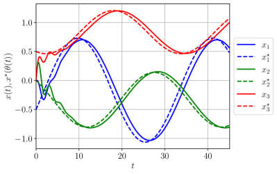
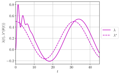
Figure 1: Plots of trajectories of the dynamics (37) solving the equality-constrained minimization problem (36). The left figure shows the trajectories of the $3$ primal variables $x(t)$ as solid curves and the trajectories of the instantaneously optimal primal variables $x^{\star}(\theta(t)$ as dashed curves. The right figure shows the trajectory of the dual variable $\lambda(t)$ as a solid curve and the instaneously optimal dual variable $\lambda^{\star}(\theta(t))$ as a dashed curve.

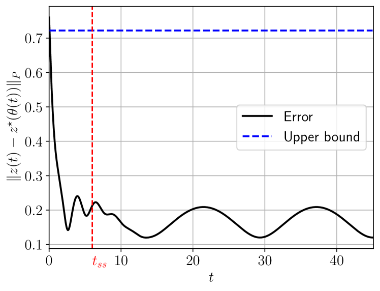
Figure 2: Plot of the error $\|z(t)-z^{\star}(\theta(t))\|_{P}$ along with the upper bound $\omega\ell/c^{2}$ where $z(t)=(x(t),\lambda(t))$ and $z^{\star}(\theta(t))=(x^{\star}(\theta(t)),\lambda^{\star}(\theta(t)))$. We also denote $3$ time-constants by $t_{\textup{ss}}$, where one time-constant is $1/c=2$ units of time.

Proposition 7.

Suppose Assumption 6 holds, let $z=(x,\lambda)\in^{n+m}$, and let $\mathsf{F}_{\textup{PAL}}:^{n+m}\times\Theta\rightarrow^{n+m}$ be the vector field defining $\dot{z}=\mathsf{F}_{\textup{PAL}}(z,\theta)$ via the dynamics (34).

1. For fixed $z\in^{n+m}$, the map $\theta\mapsto\mathsf{F}_{\textup{PAL}}(z,\theta)$ is Lipschitz from $(\Theta,\|\cdot\|_{\Theta})$ to $(^{n+m},\|\cdot\|_{P})$ with estimate

   $$\operatorname{Lip}_{\theta}(\mathsf{F}_{\textup{PAL}}){\leq}\sqrt{\chi(P)(\operatorname{Lip}_{\theta}(\nabla f)^{2}{+}\Big{(}\frac{a_{\textup{max}}}{\gamma^{2}}{+}1\Big{)}\operatorname{Lip}_{\theta}(\mathrm{prox}_{\gamma g})^{2})},$$ (35)

   where $\chi(P)$ denotes the condition number of $P$ defined in (26). We denote the right-hand side of (35) by $\ell_{\theta}$.

2. Let $\theta:\mathbb{R}_{\geq 0}\rightarrow\Theta$ be continuously differentiable. Then for any $x_{0}\in^{n},\lambda_{0}\in^{m}$ and any trajectory $z=(x,\lambda)\in^{n+m}$ satisfying $\dot{z}(t)=\mathsf{F}_{\textup{PAL}}(\theta(t),z(t))$ with $z(0)=(x_{0},\lambda_{0})$, further satisfies

   $$\left\|\begin{bmatrix}x(t)-x^{\star}(\theta(t))\\ \lambda(t)-\lambda^{\star}(\theta(t))\end{bmatrix}\right\|_{P}\leq e^{-c^{\star}t}\left\|\begin{bmatrix}x_{0}-x^{\star}(\theta(0))\\ \lambda_{0}-\lambda^{\star}(\theta(0))\end{bmatrix}\right\|_{P}\\ +\frac{\ell_{\theta}}{c^{\star}}\int_{0}^{t}e^{-c^{\star}(t-\tau)}\|\dot{\theta}(\tau)\|_{\Theta}d\tau,$$

   where $P$ is defined in (26), ${c^{\star}>0}$ is the optimal parameter solving (25), and $\ell_{\theta}$ is the right-hand side of (35).

Proof 5.20.

Regarding item (i), let $\theta,\varphi\in\Theta$, $y=Ax+\gamma\lambda\in^{m}$. Following analogous steps to the proof of 6(i)

$$\left\|\begin{bmatrix}-\nabla f_{\theta}(x)-A^{\top}\nabla M_{\gamma g_{\theta}}(y)+\nabla f_{\varphi}(x)+A^{\top}M_{\gamma g_{\varphi}}(y)\\ -\gamma\lambda+\gamma\nabla M_{\gamma g_{\theta}}(y)+\gamma\lambda-\gamma M_{\gamma g_{\varphi}}(y)\end{bmatrix}\right\|_{P}^{2}$$

$$\leq\chi(P)\Big{(}\|A^{\top}(\nabla M_{\gamma g_{\theta}}(y)\!-\!\nabla M_{\gamma g_{\varphi}}(y))\|_{2}^{2}$$

$$\quad+\|\nabla f_{\theta}(x){-}\nabla f_{\varphi}(x)\|_{2}^{2}\!+\!\|\gamma(\nabla M_{\gamma g_{\theta}}(y){-}\nabla M_{\gamma g_{\varphi}}(y))\|_{2}^{2}\Big{)}$$

$$\leq\chi(P)\Big{(}\operatorname{Lip}_{\theta}(\nabla f)^{2}{+}\Big{(}\frac{a_{\textup{max}}}{\gamma^{2}}{+}1\Big{)}\operatorname{Lip}_{\theta}(\mathrm{prox}_{\gamma g})^{2}\Big{)}\|\theta-\varphi\|_{\Theta}^{2},$$

where the final inequality holds because $\nabla M_{\gamma g_{\theta}}(y)=\frac{1}{\gamma}(y-\mathrm{prox}_{\gamma g_{\theta}}(y))$. Thus the Lipschitz estimate is proved. Item (ii) is a consequence of Theorem 3.3 where Theorem 4.15 proves strong infinitesimal contractivity in $z$ with rate $c^{\star}$ and item (i) proves Lipschitzness in $\theta$ with estimate $\ell_{\theta}$.

6 Numerical Simulations

In this section, we report two numerical examples to showcase the performance of the proposed dynamics. We present the case with equality constraints, which corresponds to Problem 3 and a case with inequality constraints, which corresponds to Problem 4. In each of these problems, we leverage the specifics of the optimization problem and corresponding dynamics to yield sharper estimates on the tracking error.

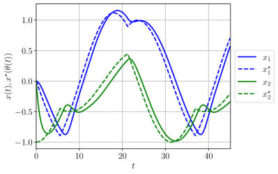
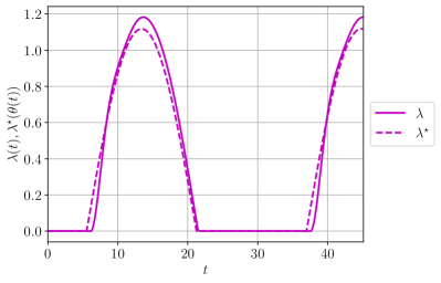
Figure 3: Plots of trajectories of the dynamics (39) solving the inequality-constrained minimization problem (38). The left figure shows the trajectories of the $2$ primal variables $x(t)$ as solid curves and the trajectories of the instantaneously optimal primal variables $x^{\star}(\theta(t)$ as dashed curves. The right figure shows the trajectory of the dual variable $\lambda(t)$ as a solid curve and the instaneously optimal dual variable $\lambda^{\star}(\theta(t))$ as a dashed curve.

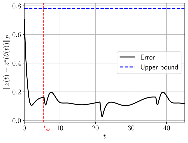
Figure 4: Plot of the error $\|z(t)-z^{\star}(\theta(t))\|_{P}$ along with the upper bound $\omega\ell/c^{2}$ where $z(t)=(x(t),\lambda(t))$ and $z^{\star}(\theta(t))=(x^{\star}(\theta(t)),\lambda^{\star}(\theta(t)))$. We also denote $3$ time-constants by $t_{\textup{ss}}$, where one time-constant is $1/c\approx 1.78$ units of time.

6.1 Equality Constraints

Consider the following quadratic optimization problem with equality constraints

$$\min_{x\in^{3}} \frac{1}{2}\|x-r(t)\|_{2}^{2},$$ (36)

s.t. $$x_{1}+2x_{2}+x_{3}=\sin(\omega t),$$

where $\omega=0.2$ and $r(t)=(\sin(\omega t),\cos(\omega t),1)$. We can see that (36) is an instance of (31) with $n=3$ primal variables and $m=1$ equality constraints by letting $\theta(t)=(\cos(\omega t),\sin(\omega t))\in\Theta:=\{z\in^{2}\;|\;\|z\|_{2}\leq 1\}\subset^{2}$. Letting $\|\cdot\|_{\Theta}=\|\cdot\|_{2}$, we can verify that Assumption 5 is verified for $f_{\theta(t)}(x)=\frac{1}{2}\|x-r(t)\|_{2}^{2}$ and $b_{\theta(t)}=\sin(\omega t)$. The corresponding primal-dual dynamics for problem (36) read

$$\dot{x}_{1} =-x_{1}+\sin(\omega t)-\lambda,$$ (37)

$$\dot{x}_{2} =-x_{2}+\cos(\omega t)-2\lambda,$$

$$\dot{x}_{3} =-x_{3}+1-\lambda,$$

$$\dot{\lambda} =x_{1}+2x_{2}+x_{3}-\sin(\omega t),$$

i.e., the dynamics are that of a linear system.

We simulate the dynamics (37) over the time interval $t\in[0,45]$ with a forward Euler discretization with stepsize $\Delta t=0.01$ and set the initial conditions $x(0)=\mathbbold{0}_{3},\lambda(0)=0$. We plot the trajectories of the dynamics along with the instantaneously optimal values $x^{\star}(\theta(t)),\lambda^{\star}(\theta(t))$ in Figure 1.

We empirically observe how the trajectories of the dynamics track the instantaneously optimal values $x^{\star}(\theta(t)),\lambda^{\star}(t)$ after a small transient. We then verify that the bound from Theorem 3.3 provides valid upper bounds for the tracking error. Finding the norm with respect to which the stable linear system (37) is contracting with largest rate corresponds to a bisection algorithm and is detailed in [6, Lemma 2.29]. After executing the bisection algorithm, we find that the primal-dual dynamics for (36) are strongly infinitesimally contracting with respect to $\|\cdot\|_{P}$ with rate $c=0.5$ for suitably chosen $P=P^{\top}\succ 0$. Then the corresponding Lipschitz constant for the vector field is computed from $(\Theta,\|\cdot\|_{2})$ to $(^{4},\|\cdot\|_{P})$, and is approximately $\ell\approx 0.902$. From Theorem 3.3, we know that the asymptotic tracking error as measured in the $\|\cdot\|_{P}$ norm is upper bounded by $\frac{\ell}{c^{2}}\omega\approx 0.722$ since $\|\dot{\theta}(t)\|_{2}=\omega$ for all $t\geq 0$. In Figure 2 we plot $\left\|z(t)-z^{\star}(\theta(t))\right\|_{P}$ where $z$ is the stacked vector of $x$ and $\lambda$ as well as the upper bound $\frac{\ell}{c^{2}}\omega$ to demonstrate the validity of our bound.

Remark 6.21.

Note that in this example we have leveraged the fact that the dynamics (37) are linear to get improved rates of contraction. If we had instead simply used the bound on the contraction rate from Theorem 4.12, we would instead have $c=\frac{5}{18}$, which would yield looser bounds on the asymptotic error (measured in a different norm, however). $\triangle$

6.2 Inequality Constraints

Consider the following quadratic optimization problem with inequality constraints

$$\min_{x\in^{2}} \frac{1}{2}\|x+r(t)\|_{2}^{2},$$ (38)

s.t. $${-}x_{1}+x_{2}\leq\cos(\omega t),$$

where ${\omega=0.2}$ and ${r(t)=(\sin(\omega t),\cos(\omega t))}$. We see that (38) is an instance of (34) with ${g:\times\Theta\rightarrow\overline{}}$ given by ${g(z,\theta)=\iota_{\mathcal{C}_{\theta}}(z)}$ where ${\mathcal{C}_{\theta}=\{z\in\;|\;z\leq\theta_{1}\}}$, $\theta(t)={(\cos(\omega t),\sin(\omega t))\in\Theta:=\{z\in^{2}\;|\;\|z\|_{2}\leq 1\}}$, and ${A=[-1,1]}$. Then for given $t,\theta(t),z$, we can verify that ${\mathrm{prox}_{\gamma g_{\theta(t)}}(z)=\operatorname{P}_{\mathcal{C}_{\theta(t)}}(z)=\min\{z,\cos(\omega t)\}}$ and the corresponding Moreau envelope is $\nabla M_{\gamma g_{\theta(t)}}(z)=\frac{1}{\gamma}(z-\min\{z,\cos(\omega t)\})=\frac{1}{\gamma}\mathrm{ReLU}(z-\cos(\omega(t)))$. Thus, we can verify that Assumption 6 is satisfied for the optimization problem (38).

The corresponding primal-dual dynamics on the augmented Lagrangian for the minimization problem (38) then read

$$\dot{x}_{1} =-x_{1}-\sin(\omega t)+\frac{1}{\gamma}\mathrm{ReLU}(-x_{1}+x_{2}+\gamma\lambda-\cos(\omega t)),$$

$$\dot{x}_{2} =-x_{2}-\cos(\omega t)-\frac{1}{\gamma}\mathrm{ReLU}(-x_{1}+x_{2}+\gamma\lambda-\cos(\omega t)),$$

$$\dot{\lambda} =-\gamma\lambda+\mathrm{ReLU}(-x_{1}+x_{2}+\gamma\lambda-\cos(\omega t)).$$ (39)

We simulate the dynamics (39) with $\gamma=10$ over the time interval $t\in[0,45]$ with a forward Euler discretization with stepsize $\Delta t=0.01$ and initial conditions ${x(0)=\mathbbold{0}_{2},\lambda(0)=0}$. We plot the trajectories of the dynamics along with the instantaneously optimal values $x^{\star}(\theta(t)),\lambda^{\star}(\theta(t))$ in Figure 3.

We empirically observe how the trajectories of the dynamics track the instantaneously optimal values $x^{\star}(\theta(t)),\lambda^{\star}(t)$ after a small transient. We then verify that the bound from Theorem 3.3 provides a valid upper bound for the tracking error. Note that the vector field for the dynamics (39) is almost everywhere differentiable and its Jacobian has the structure

$$D\mkern-0.75mu{\mathsf{F}_{\textup{PAL}}}(z)=\begin{bmatrix}-1-\frac{1}{\gamma}J&\frac{1}{\gamma}J&J\\ \frac{1}{\gamma}J&-1-\frac{1}{\gamma}J&-J\\ -J&J&-\gamma+\gamma J\end{bmatrix},$$ (40)

where $J$ denotes the derivative of the $\mathrm{ReLU}$ evaluated at $-x_{1}+x_{2}+\gamma\lambda-\cos(\omega t)$ and always takes value in $\{0,1\}$ when it is defined. In other words, the Jacobian always takes one of two values. Finding the norm which maximizes the contraction rate of the dynamics (39) corresponds to the minimization problem

$$\min_{c\in,P\in^{3\times 3}} c,$$ (41)

s.t. $$PD_{i}+D_{i}^{\top}P\preceq 2cP,\quad i\in\{1,2\},$$

$$P=P^{\top}\succ 0,$$

where $D_{1}$ corresponds to the Jacobian (40) with $J=1$ and $D_{2}$ corresponds to the Jacobian (40) with $J=0$. The problem (41) can be solved using a bisection algorithm on $c$ as discussed in [6, Lemma 2.29]. After running the bisection algorithm, we find that the dynamics (39) are strongly infinitesimally contracting with respect to $\|\cdot\|_{P}$ with rate $c=0.5625$ for suitably chosen $P=P^{\top}\succ 0$. Then the corresponding Lipschitz constant for the vector field is computed from $(\Theta,\|\cdot\|_{2})$ to $(^{3},\|\cdot\|_{P})$ and is approximately $\ell\approx 1.235$. From Theorem 3.3, we know that the asymptotic tracking error as measured in the $\|\cdot\|_{P}$ norm is upper bounded by $\frac{\ell}{c^{2}}\omega\approx 0.781$ since $\|\dot{\theta}(t)\|_{2}=\omega$ for all $t\geq 0$. In Figure 4 we plot $\left\|z(t)-z^{\star}(\theta(t))\right\|_{P}$ as well as the upper bound $\frac{\ell}{c^{2}}\omega$ to demonstrate the validity of our bound.

Remark 6.22.

As in the previous example, we leverage the specific structure of the dynamics (39) to yield sharper bounds on the contraction rate $c$ instead of using the nonlinear program (25). $\triangle$

7 Discussion

In this article, we take a contraction theory approach to the problem of tracking optimal trajectories in time-varying convex optimization problems. We prove in Theorem 3.3 that the tracking error between any solution trajectory of a strongly infinitesimally contracting system and its equilibrium trajectory is upper bounded with an explicit estimate on the bound. To apply this Theorem, we establish the strong infinitesimal contractivity of three dynamical systems solving optimization problems and apply Theorem 3.3 to provide explicit tracking error bounds. We validate these bounds in two numerical examples.

We believe that this work motivates future research in establishing the strong infinitesimal contractivity of dynamical systems solving optimization problems or performing more general computation due to the desirable consequences of contractivity. As future research, we plan to investigate (i) discretization of parameter-varying contracting dynamics and establish similar tracking error bounds for discrete-time contracting systems, (ii) contractivity properties of continuous-time stochastic optimization algorithms based on stochastic differential equations [1], and (iii) nonconvex optimization problems with isolated local minima using the theory of $k$-contraction [35].

8 Proofs and Additional Results

First, we present a result on the Lipschitzness of parametrized time-varying equilibrium trajectories and a bound on their time derivatives.

Lemma 8.23 (Lipschitzness of parametrized curves).

Consider $\mathcal{X}\subseteq\mathbb{R}^{n}$ and $\mathcal{U}\subseteq\mathbb{R}^{d}$ with associated norms $\|\cdot\|_{\mathcal{X}}:\mathbb{R}^{n}\rightarrow\mathbb{R}_{\geq 0}$ and $\|\cdot\|_{\mathcal{U}}:\mathbb{R}^{d}\rightarrow\mathbb{R}_{\geq 0}$, respectively. Let ${G:\mathcal{U}\rightarrow\mathcal{X}}$ be Lipschitz from $(\mathcal{U},\|\cdot\|_{\mathcal{U}})$ to $(\mathcal{X},\|\cdot\|_{\mathcal{X}})$ with constant $\operatorname{Lip}(G)\geq 0$. Then for every $a,b\in$ with $a<b$ and every continuously differentiable $u:{]a,b[}\rightarrow\mathcal{U}$,

1. the curve $x:{]a,b[}\rightarrow\mathcal{X}$ given by $x(t)=G(u(t))$ is locally Lipschitz;

2. $\|\dot{x}(t)\|_{\mathcal{X}}\leq\operatorname{Lip}(G)\|\dot{u}(t)\|_{\mathcal{U}}$, for a.e. $t\in{]a,b[}$.

Proof 8.24.

Item (i) is a consequence of the fact that continuously differentiable mappings are locally Lipschitz and that a composition of Lipschitz mappings is Lipschitz.

To prove item (ii) we first note that item (i) implies that $\dot{x}(t)$ exists almost everywhere by Rademacher’s theorem. Next, for all $t\in{]a,b[}$ for which $\dot{x}(t)$ exists,

$$\|\dot{x}(t)\|_{\mathcal{X}} {=}\Big{\|}\lim_{h\to 0^{+}}\!\!\!\frac{x(t+h){-}x(t)}{h}\Big{\|}_{\mathcal{X}}\!{=}\!\lim_{h\to 0^{+}}\!\!\frac{1}{h}\|x(t+h){-}x(t)\|_{\mathcal{X}}$$

$${\leq}\lim_{h\to 0^{+}}\frac{\operatorname{Lip}(G)}{h}\|u(t+h){-}u(t)\|_{\mathcal{U}}$$

$${=}\operatorname{Lip}(G)\Big{\|}\lim_{h\to 0^{+}}\!\!\!{\frac{u(t+h){-}u(t)}{h}}\Big{\|}_{\mathcal{U}}{=}\operatorname{Lip}(G)\|\dot{u}(t)\|_{\mathcal{U}},$$

where we have used the continuity of $\|\cdot\|_{\mathcal{X}}$ and $\|\cdot\|_{\mathcal{U}}$ and the Lipschitzness of $G$.

Proof 8.25 (Proof of Lemma 1).

Consider the dynamical systems $\dot{x}=F(x,u)$ where $u$ is constant. [6, Theorem 3.9] implies that there exists a unique point $x_{u}^{\star}\in\mathcal{X}$ satisfying the equilibrium equation $F(x_{u}^{\star},u)=\mbox{0}_{n}$. Let $x^{\star}:\mathcal{U}\rightarrow\mathcal{X}$ denote the map given by $x^{\star}(u)=x_{u}^{\star}$. Given two constant inputs $u$ and $v$, the two equilibrium solutions are $x^{\star}(u)$ and $x^{\star}(v)$. The assumptions of [6, Theorem 3.16] are satisfied with $c=-\operatorname{osL}_{x}(F)$ and $\ell_{u}=\operatorname{Lip}_{u}(F)$, and the differential inequality [6, equation 3.39] implies

$$0\leq-c\|x^{\star}(u)-x^{\star}(v)\|_{\mathcal{X}}+\ell_{u}\|u-v\|_{\mathcal{U}}.$$

This concludes the proof.

Lemma 8.26.

Let $\mathsf{T}:^{n}\rightarrow^{n}$ be Lipshitz with respect to a norm $\|\cdot\|$ with constant $\operatorname{Lip}(\mathsf{T})$. Then the vector field $F:^{n}\rightarrow^{n}$ defined by the dynamics

$$\dot{x}=-x+\mathsf{T}(x)=:F(x)$$ (42)

satisfies $\operatorname{osL}(F)\leq-1+\operatorname{Lip}(\mathsf{T})$. Moreover, if $\operatorname{Lip}(\mathsf{T})<1$, then $\mathsf{T}$ has a unique fixed point, $x^{*}$, which is the unique equilibrium point of the contracting dynamics (42).

Proof 8.27.

We have that $\operatorname{osL}(F):=\operatorname{osL}(-\mathsf{Id}+\mathsf{T})=-1+\operatorname{osL}(\mathsf{T})\leq-1+\operatorname{Lip}(\mathsf{T})$, where we have used the translation property of $\operatorname{osL}$ and the upper bound $\operatorname{osL}(\mathsf{T})\leq\operatorname{Lip}(\mathsf{T})$ [6, Sec. 3.2.3]. If $\operatorname{Lip}(\mathsf{T})<1$, the Banach contraction theorem implies the existence of a unique fixed point and equilibrium points of (42) are exactly fixed points of $\mathsf{T}$. Moreover, the dynamics (42) are contracting since $\operatorname{osL}(F)<0$.

Lemma 8.28 (Symmetry and bounds on Jacobians).

Let the map ${g:^{n}\rightarrow\overline{}}$ be CCP. Then for every $\gamma>0$, $D\mkern-0.75mu{\mathrm{prox}_{\gamma g}}(x)$ and $\nabla^{2}M_{\gamma g}(x)$ exist for a.e. $x\in^{n}$, are symmetric, and satisfy

$$0\preceq D\mkern-0.75mu{\mathrm{prox}_{\gamma g}}(x)\preceq I_{n},\quad 0\preceq\nabla^{2}M_{\gamma g}(x)\preceq\frac{1}{\gamma}I_{n}.$$ (43)

Proof 8.29.

First note that $D\mkern-0.75mu{\mathrm{prox}_{\gamma g}}(x)$ and $\nabla^{2}M_{\gamma g}(x)$ exist for a.e. $x\in^{n}$ by Rademacher’s theorem since $\mathrm{prox}_{\gamma g}$ and $\nabla M_{\gamma g}$ are both Lipschitz. Furthermore, $\nabla^{2}M_{\gamma g}(x)$ is symmetric for a.e. $x$ by symmetry of second derivatives. Analogously, $D\mkern-0.75mu{\mathrm{prox}_{\gamma g}}(x)=x-\alpha\nabla^{2}M_{\gamma g}(x)$ by formula (4) so we conclude symmetry of $D\mkern-0.75mu{\mathrm{prox}_{\gamma g}}(x)$ as well. The bounds (43) are a consequence of the fact that $\mathrm{prox}_{\gamma g}$ and $\mathsf{Id}-\mathrm{prox}_{\gamma g}$ are both firmly nonexpansive [3, Proposition 12.28].

9 Logarithmic norm of Hurwitz saddle matrices

Lemma 9.30 (Logarithmic norm of Hurwitz saddle matrices).

Given $B=B^{\top}\in^{n\times n}$ and $A\in^{m\times n}$, with $m\leq n$, we consider the saddle matrix

$$\mathcal{B}=\begin{bmatrix}-B&-A^{\top}\\ A&0\end{bmatrix}\in^{(m+n)\times(m+n)}.$$ (44)

Then, for each matrix pair $(B,A)$ satisfying $\rho I_{n}\preceq B\preceq\ell I_{n}$ and $a_{\textup{min}}I_{m}\preceq AA^{\top}\preceq a_{\textup{max}}I_{m}$, for $\rho,\ell,a_{\textup{min}},a_{\textup{max}}\in\mathbb{R}_{>0}$, the following contractivity LMI holds:

$$\mathcal{B}^{\top}P+P\mathcal{B}\preceq-2cP\quad\iff\quad\mu_{P}(\mathcal{B})\leq-c,$$ (45)

where

$$P =\begin{bmatrix}I_{n}&\alpha A^{\top}\\ \alpha A&I_{m}\end{bmatrix}\succ 0,\ \alpha=\frac{1}{3}\min\Big{\{}\frac{1}{\ell},\frac{\rho}{a_{\textup{max}}}\Big{\}},\ \text{and}$$ (46)

$$c =\frac{5}{6}\alpha a_{\textup{min}}=\frac{5}{18}\min\Big{\{}\frac{a_{\textup{min}}}{\ell},\frac{a_{\textup{min}}}{a_{\textup{max}}}\rho\Big{\}}.$$ (47)

Proof 9.31.

We start by verifying that $P\succ 0$. Using the Schur complement of the $(2,2)$ entry, we need to verify that

$$I_{n}-\alpha^{2}A^{\top}A\succ 0\iff 1-\alpha^{2}a_{\textup{max}}>0\iff\alpha^{2}<1/a_{\textup{max}}.$$

The inequality $\alpha^{2}<1/a_{\textup{max}}$ follows from the tighter inequality $(3\alpha)^{2}\leq\displaystyle\tfrac{1}{a_{\textup{max}}}$ which is proved as follows:

$$\min\Big{\{}\frac{1}{\ell},\frac{\rho}{a_{\textup{max}}}\Big{\}}^{2} \leq\min\Big{\{}\frac{1}{\ell},\frac{\rho}{a_{\textup{max}}}\Big{\}}\cdot\max\Big{\{}\frac{1}{\ell},\frac{\rho}{a_{\textup{max}}}\Big{\}}$$

$$=\frac{1}{\ell}\cdot\frac{\rho}{a_{\textup{max}}}\leq\frac{1}{a_{\textup{max}}}.$$

Next, we aim to show that $Q:={-}\mathcal{B}^{\top}P-P\mathcal{B}-2cP\succeq 0$. After some bookkeeping, we compute

$$Q=\begin{bmatrix}2B{-}2\alpha A^{\top}A{-}2cI_{n}&\alpha BA^{\top}{-}2c\alpha A^{\top}\\ A{+}\alpha AB{-}A{-}2c\alpha A&2\alpha AA^{\top}{-}2cI_{m}\end{bmatrix}.$$

The (2,2) block satisfies the lower bound

$$2\alpha AA^{\top}{-}2cI_{m} =2\big{(}\tfrac{5}{6}\alpha AA^{\top}{-}cI_{m}\big{)}+\tfrac{1}{3}\alpha AA^{\top}$$

$$\!\!\succeq 2\big{(}\tfrac{5}{6}\alpha a_{\textup{min}}{-}c\big{)}I_{m}+\tfrac{1}{3}\alpha AA^{\top}{=}\tfrac{1}{3}\alpha AA^{\top}\succ 0.$$

Given this lower bound, we can factorize the resulting matrix as follows:

$$Q={-}\mathcal{B}^{\top}P-P\mathcal{B}-2cP\\ \succeq\begin{bmatrix}I_{n}&\!\!0\\ 0&\!\!A\end{bmatrix}\underbrace{\begin{bmatrix}2B{-}2(\alpha A^{\top}A+cI_{n})&\!\alpha B{-}2c\alpha I_{n}\\ \alpha B{-}2c\alpha I_{n}&\!\tfrac{1}{3}\alpha I_{n}\end{bmatrix}}_{n\times n}\begin{bmatrix}I_{n}&\!\!0\\ 0&\!\!A^{\top}\end{bmatrix}.$$

Since $\tfrac{1}{3}\alpha I_{n}\succ 0$, it now suffices to show that the Schur complement of the (2,2) block of $n\times n$ matrix is positive semidefinite. We proceed as follows:

$$2B-2(\alpha A^{\top}A+cI_{n})-3\alpha\big{(}B-2cI_{n}\big{)}^{2}\succeq 0$$

$$\!\!\!\iff\!\!2B-3\alpha B^{2}+12\alpha cB\succeq 2(\alpha A^{\top}A+cI_{n})+12\alpha c^{2}I_{n}$$

$$\!\!\!\impliedby 2B-3\alpha B^{2}\succeq 2(\alpha A^{\top}A+cI_{n})\ \text{and}\ 12\alpha cB\succeq 12\alpha c^{2}I_{n}.$$

To prove $2B-3\alpha B^{2}\succeq 2(\alpha A^{\top}A+cI_{n})$, we upper bound the right hand side as follows:

$$2(\alpha A^{\top}A+cI_{n}) \overset{\eqref{def:P-alpha+c}}{\preceq}\alpha(2a_{\textup{max}}+a_{\textup{min}})I_{n}$$

$$\!\!\!\!\!\!\!\!\!\overset{\alpha\leq\tfrac{1}{3}\rho/a_{\textup{max}}}{\preceq}\frac{1}{3}\frac{\rho}{a_{\textup{max}}}(2a_{\textup{max}}+a_{\textup{min}})I_{n}\preceq\rho I_{n}.$$

Next, since $\alpha\leq\frac{1}{3\ell}$, we know $-3\alpha\ell\geq-1$. We then upper bound the left hand side as follows:

$$2B-3\alpha B^{2} \succeq 2B-3\alpha\ell B\succeq(2-1)B\succeq\rho I_{n}.$$

Finally, the inequality $12\alpha cB\succeq 12\alpha c^{2}I_{n}$ follows from noting $c\leq\tfrac{5}{18}\tfrac{a_{\textup{min}}}{a_{\textup{max}}}\rho<\rho$.

10 Generalized Saddle Matrices

The following lemma is presented in [25, Lemma 6]. We include it here for completeness.

Lemma 10.32.

Let $X=X^{\top}\in^{m\times m}$ satisfy $0\preceq X\preceq x_{\max}I_{m}$ for some $x_{\max}>0$, $\gamma>0$, and $\displaystyle\alpha\leq\frac{\gamma}{x_{\max}}$. Then for all $d\in[0,1]^{m}$, the following inequality holds

$$\alpha(\mathrm{diag}(d)X+X\mathrm{diag}(d))+2\gamma(I_{m}-\mathrm{diag}(d))\succeq\frac{3}{2}\alpha X.$$ (48)

Proof 10.33.

See [25, Lemma 6].

The following lemma is a generalization of [25, Lemma 4], where we let the matrix $G$ be dense. The proof method is otherwise similar with a few improved bounds.

Lemma 10.34 (Generalized saddle matrices).

Given $A\in^{m\times n}$, ${B=B^{\top}\in^{n\times n}}$, and $G=G^{\top}\in^{m\times m}$, with $m\leq n$, and $\gamma>0$, we consider the saddle matrix

$$\mathcal{B}=\begin{bmatrix}-B-\frac{1}{\gamma}A^{\top}GA&-A^{\top}G\\ GA&-\gamma(I_{m}-G)\end{bmatrix}\in^{(m+n)\times(m+n)}.$$ (49)

Then, for each matrix triplet $(B,A,G)$ satisfying $\rho I_{n}\preceq B\preceq\ell I_{n}$, $a_{\textup{min}}I_{m}\preceq AA^{\top}\preceq a_{\textup{max}}I_{m}$, and $0\preceq G\preceq I_{m}$, for $\rho$, $\ell$, $a_{\textup{min}}$, $a_{\textup{max}}\in\mathbb{R}_{>0}$, the following contractivity LMI holds:

$$\mathcal{B}^{\top}P+P\mathcal{B}\preceq-2c^{\star}P\quad\iff\quad\mu_{P}(\mathcal{B})\leq-c^{\star},$$ (50)

where

$$P=\begin{bmatrix}I_{n}&\alpha^{\star}A^{\top}\\ \alpha^{\star}A&I_{m}\end{bmatrix}\succ 0,$$ (51)

and $c^{\star}$ and $\alpha^{\star}$ are the optimal parameters for the problem (25).

Proof 10.35.

Define the matrix $Q\in^{(m+n)\times(m+n)}$ by

$$Q=-\mathcal{B}^{\top}P-P\mathcal{B}-2c^{\star}P=\begin{bmatrix}Q_{11}&Q_{12}\\ Q_{12}^{\top}&Q_{22}\end{bmatrix},$$ (52)

where $Q_{11}\in^{n\times n}$, $Q_{12}\in^{n\times m}$, and $Q_{22}\in^{m\times m}$. We aim to show that $Q\succeq 0$ for $c^{\star}$ and $\alpha^{\star}$ optimal parameters for the problem (25). We have

$$Q_{11} =2B+\Big{(}\frac{2}{\gamma}-2\alpha^{\star}\Big{)}A^{\top}GA-2c^{\star}I_{n},$$

$$Q_{12} =\alpha^{\star}\gamma A^{\top}(I_{m}{-}G){+}\alpha^{\star}BA^{\top}{+}\frac{\alpha^{\star}}{\gamma}A^{\top}GAA^{\top}{-}2c^{\star}\alpha^{\star}A^{\top},$$

$$Q_{22} =\alpha^{\star}(AA^{\top}G+GAA^{\top})+2\gamma(I_{m}-G)-2c^{\star}I_{m}.$$

To show that $Q\succeq 0$ we use the Schur Complement, which requires to prove that $Q_{22}\succ 0$ and $Q_{11}-Q_{12}Q_{22}^{-1}Q_{12}^{\top}\succeq 0$. We do this in three steps.

First, we find a lower bound for $Q_{22}$. Since $G$ is symmetric and satisfies $0\preceq G\preceq I_{m}$, there exists an orthogonal matrix $U\in^{m\times m}$ and $d\in[0,1]^{m}$ such that $G=U\mathrm{diag}(d)U^{\top}$. Substituting this into $Q_{22}$ and multiplying on the left and on the right by $U$ and $U^{\top}$, respectively, we get

$$U^{\top}Q_{22}U =\alpha^{\star}(U^{\top}AA^{\top}U\mathrm{diag}(d)+\mathrm{diag}(d)U^{\top}AA^{\top}U)$$

$$\quad+2\gamma(I_{m}-\mathrm{diag}(d))-2c^{\star}I_{m},$$ (53)

where we have used the fact that $U\in\mathbb{R}^{m\times m}$ orthogonal, i.e., ${UU^{\top}=U^{\top}{U}=I_{m}}$. Moreover, the orthogonality of $U$ implies that ${U^{-1}=U^{\top}}$. Thus the eigenvalues of $U^{\top}AA^{\top}U$ and $AA^{\top}$ are equal, and therefore, $a_{\textup{min}}I_{m}\preceq U^{\top}AA^{\top}U\preceq a_{\textup{max}}I_{m}$. Next, applying Lemma 10.32 to (10.35), with $X:=U^{\top}AA^{\top}U$, and, multiplying this on the left and on the right by $U$ and $U^{\top}$, respectively, we get the following lower bound

$$Q_{22}\succeq\frac{3}{2}\alpha^{\star}AA^{\top}-2c^{\star}I_{m},$$ (54)

where the inequality holds because $\alpha^{\star}\leq\frac{\gamma}{a_{\textup{max}}}$ – constraint (25b). Finally, we note that $Q_{22}\succ 0$ for $\alpha^{\star}$ and $c^{\star}$ optimal parameters for the problem (25)

Next, we need to prove that $Q_{11}-Q_{12}Q_{22}^{-1}Q_{12}^{\top}\succeq 0$ for $c^{\star}$ and $\alpha^{\star}$ optimal parameters for the problem (25). To this purpose, first note that for every $\kappa>\frac{2}{3}\frac{a_{\textup{max}}}{a_{\textup{min}}}\frac{1}{\alpha^{\star}}$,

$$Q_{22}\succeq\frac{1}{\kappa}AA^{\top}.$$ (55)

Next, we upper bound $Q_{12}Q_{22}^{-1}Q_{12}^{\top}$. To simplify notation, define $R_{1}=B+\frac{1}{\gamma}A^{\top}GA-2c^{\star}I_{n}\in\mathbb{R}^{n\times n}$, $R_{2}=\gamma A^{\top}(I_{m}-G)\in\mathbb{R}^{n\times m}$, and note that $Q_{12}=\alpha^{\star}(R_{1}A^{\top}+R_{2})\in\mathbb{R}^{n\times m}$. We compute

$$\!\!\!\!\!\!Q_{12}Q_{22}^{-1}Q_{12}^{\top}\!\!\overset{\eqref{eq:bound_Q22}}{\preceq}\kappa Q_{12}(AA^{\top})^{-1}Q_{12}$$

$$\preceq(\alpha^{\star})^{2}\kappa(R_{1}A^{\top}(AA^{\top})^{-1}AR^{\top}_{1}{+}R_{1}A^{\top}(AA^{\top})^{-1}R^{\top}_{2}$$

$$\quad+R_{2}(AA^{\top})^{-1}AR^{\top}_{1}+R_{2}(AA^{\top})^{-1}R^{\top}_{2})$$

$$\preceq(\alpha^{\star})^{2}\kappa(R_{1}R^{\top}_{1}+2\|R_{1}A^{\top}(AA^{\top})^{-1}R^{\top}_{2}\|I_{n}$$

$$\quad+\|R_{2}(AA^{\top})^{-1}R^{\top}_{2}\|I_{n}),$$ (56)

where the final inequality holds because $A^{\top}(AA^{\top})^{-1}A\preceq I_{n}$. Note that

$$R_{1}R^{\top}_{1} \preceq\ell^{2}I_{n}{+}\Big{(}2\ell{+}\frac{a_{\textup{max}}}{\gamma}{+}2c^{\star}\Big{)}\Big{(}\frac{a_{\textup{max}}}{\gamma}{+}2c^{\star}\Big{)}I_{n}{=:}h_{1}(c^{\star})I_{n},$$

where we have introduced the function ${h_{1}:\mathbb{R}_{\geq 0}\rightarrow\mathbb{R}_{\geq 0}}$ defined by $h_{1}(c^{\star})=\ell^{2}+2\ell(\frac{a_{\textup{max}}}{\gamma}+2c^{\star})+(\frac{a_{\textup{max}}}{\gamma}+2c^{\star})^{2}$. Moreover,

$$\|R_{2}(AA^{\top})^{-1}R^{\top}_{2}\| \leq\gamma^{2}\frac{a_{\textup{max}}}{a_{\textup{min}}},\text{ and }$$

$$2\|R_{1}A^{\top}(AA^{\top})^{-1}R^{\top}_{2}\| \leq 2\gamma\frac{a_{\textup{max}}}{a_{\textup{min}}}\Big{(}\ell{+}\frac{a_{\textup{max}}}{\gamma}{+}2c^{\star}\Big{)}=:h_{2}(c^{\star}),$$

where, we have introduced the function ${h_{2}:\mathbb{R}_{\geq 0}\rightarrow\mathbb{R}_{\geq 0}}$ defined by $h_{2}(c^{\star}):=2\gamma\frac{a_{\textup{max}}}{a_{\textup{min}}}(\ell+\frac{a_{\textup{max}}}{\gamma}+2c^{\star})$. Substituting the previous bounds on the LMI (56) we get

$$Q_{12}Q_{22}^{-1}Q_{12}^{\top}\preceq(\alpha^{\star})^{2}\kappa\Big{(}h_{1}(c^{\star})+h_{2}(c^{\star})+\gamma^{2}\frac{a_{\textup{max}}}{a_{\textup{min}}}\Big{)}I_{n}.$$

Next, we compute

$$Q_{11} =2B+\Big{(}\frac{2}{\gamma}-2\alpha^{\star}\Big{)}A^{\top}GA-2c^{\star}I_{n}$$

$$\succeq\Big{(}2\rho-\mathrm{ReLU}\Big{(}2\alpha^{\star}-\frac{2}{\gamma}\Big{)}a_{\textup{max}}-2c^{\star}\Big{)}I_{n}.$$

Finally, we have

$$Q_{11}{-}Q_{12}Q_{22}^{-1}Q_{12}^{\top}\succeq I_{n}\Big{(}2\rho-\mathrm{ReLU}\Big{(}2\alpha^{\star}-\frac{2}{\gamma}\Big{)}a_{\textup{max}}-2c^{\star}$$

$$\qquad-(\alpha^{\star})^{2}\kappa\Big{(}h_{1}(c^{\star})+h_{2}(c^{\star})+\gamma^{2}\frac{a_{\textup{max}}}{a_{\textup{min}}}\Big{)}\Big{)}\succeq 0,$$

where the last inequality follows from constraint (25e). This concludes the proof.

References

- [1] Z. Aminzare. Stochastic logarithmic Lipschitz constants: A tool to analyze contractivity of stochastic differential equations. IEEE Control Systems Letters, 6:2311–2316, 2022. doi:10.1109/LCSYS.2022.3148945.
- [2] K. J. Arrow, L. Hurwicz, and H. Uzawa, editors. Studies in Linear and Nonlinear Programming. Stanford University Press, 1958.
- [3] H. H. Bauschke and P. L. Combettes. Convex Analysis and Monotone Operator Theory in Hilbert Spaces. Springer, 2 edition, 2017, ISBN 978-3-319-48310-8.
- [4] G. Bianchin, J. Cortés, J. I. Poveda, and E. Dall’Anese. Time-varying optimization of LTI systems via projected primal-dual gradient flows. IEEE Transactions on Control of Network Systems, 9(1):474–486, 2022. doi:10.1109/TCNS.2021.3112762.
- [5] R. W. Brockett. Dynamical systems that sort lists, diagonalize matrices, and solve linear programming problems. Linear Algebra and its Applications, 146:79–91, 1991. doi:10.1016/0024-3795(91)90021-N.
- [6] F. Bullo. Contraction Theory for Dynamical Systems. Kindle Direct Publishing, 1.1 edition, 2023, ISBN 979-8836646806. URL: https://fbullo.github.io/ctds.
- [7] V. Centorrino, A. Gokhale, A. Davydov, G. Russo, and F. Bullo. Euclidean contractivity of neural networks with symmetric weights. IEEE Control Systems Letters, 2023. Early access. doi:10.1109/LCSYS.2023.3278250.
- [8] A. Cherukuri, B. Gharesifard, and J. Cortes. Saddle-point dynamics: Conditions for asymptotic stability of saddle points. SIAM Journal on Control and Optimization, 55(1):486–511, 2017. doi:10.1137/15M1026924.
- [9] P. Cisneros-Velarde, S. Jafarpour, and F. Bullo. Distributed and time-varying primal-dual dynamics via contraction analysis. IEEE Transactions on Automatic Control, 67(7):3560–3566, 2022. doi:10.1109/TAC.2021.3103865.
- [10] M. Colombino, E. Dall’Anese, and A. Bernstein. Online optimization as a feedback controller: Stability and tracking. IEEE Transactions on Control of Network Systems, 7(1):422–432, 2020. doi:10.1109/TCNS.2019.2906916.
- [11] J. Cortés and S. K. Niederländer. Distributed coordination for nonsmooth convex optimization via saddle-point dynamics. Journal of Nonlinear Science, 29(4):1247–1272, 2019. doi:10.1007/s00332-018-9516-4.
- [12] A. Davydov, S. Jafarpour, and F. Bullo. Non-Euclidean contraction theory for robust nonlinear stability. IEEE Transactions on Automatic Control, 67(12):6667–6681, 2022. doi:10.1109/TAC.2022.3183966.
- [13] A. Davydov, A. V. Proskurnikov, and F. Bullo. Non-Euclidean contraction analysis of continuous-time neural networks. IEEE Transactions on Automatic Control, September 2022. Submitted. doi:10.48550/arXiv.2110.08298.
- [14] N. K. Dhingra, S. Z. Khong, and M. R. Jovanović. The proximal augmented Lagrangian method for nonsmooth composite optimization. IEEE Transactions on Automatic Control, 64(7):2861–2868, 2019. doi:10.1109/TAC.2018.2867589.
- [15] M. Fazlyab, S. Paternain, V. M. Preciado, and A. Ribeiro. Prediction-correction interior-point method for time-varying convex optimization. IEEE Transactions on Automatic Control, 63(7):1973–1986, 2018. doi:10.1109/TAC.2017.2760256.
- [16] M. Fortin. Minimization of some non-differentiable functionals by the augmented Lagrangian method of Hestenes and Powell. Applied Mathematics and Optimization, 2:236–250, 1975. doi:10.1007/BF01464269.
- [17] X.-B. Gao. Exponential stability of globally projected dynamic systems. IEEE Transactions on Neural Networks, 14(2):426–431, 2003. doi:10.1109/tnn.2003.809409.
- [18] S. Hassan-Moghaddam and M. R. Jovanović. Proximal gradient flow and Douglas-Rachford splitting dynamics: Global exponential stability via integral quadratic constraints. Automatica, 123:109311, 2021. doi:10.1016/j.automatica.2020.109311.
- [19] A. Hauswirth, S. Bolognani, G. Hug, and F. Dörfler. Optimization algorithms as robust feedback controllers. arXiv e-print:2103.11329, 2021. URL: https://arxiv.org/abs/2103.11329.
- [20] J. J. Hopfield and D. W. Tank. ”Neural” computation of decisions in optimization problems. Biological Cybernetics, 52(3):141–152, 1985. doi:10.1007/bf00339943.
- [21] M. P. Kennedy and L. O. Chua. Neural networks for nonlinear programming. IEEE Transactions on Circuits and Systems, 35(5):554–562, 1988. doi:10.1109/31.1783.
- [22] W. Lohmiller and J.-J. E. Slotine. On contraction analysis for non-linear systems. Automatica, 34(6):683–696, 1998. doi:10.1016/S0005-1098(98)00019-3.
- [23] P. H. A. Ngoc and H. Trinh. On contraction of functional differential equations. SIAM Journal on Control and Optimization, 56(3):2377–2397, 2018. doi:10.1137/16M1092672.
- [24] H. D. Nguyen, T. L. Vu, K. Turitsyn, and J.-J. E. Slotine. Contraction and robustness of continuous time primal-dual dynamics. IEEE Control Systems Letters, 2(4):755–760, 2018. doi:10.1109/LCSYS.2018.2847408.
- [25] G. Qu and N. Li. On the exponential stability of primal-dual gradient dynamics. IEEE Control Systems Letters, 3(1):43–48, 2019. doi:10.1109/LCSYS.2018.2851375.
- [26] E. K. Ryu and S. Boyd. Primer on monotone operator methods. Applied Computational Mathematics, 15(1):3–43, 2016.
- [27] C. D. Schuman, S. R. Kulkarni, M. Parsa, J. P. Mitchell, P. Date, and B. Kay. Opportunities for neuromorphic computing algorithms and applications. Nature Computational Science, 2:10–19, 2022. doi:10.1038/s43588-021-00184-y.
- [28] A. Simonetto and E. Dall’Anese. Prediction-correction algorithms for time-varying constrained optimization. IEEE Transactions on Signal Processing, 65(20):5481–5494, 2017. doi:10.1109/TSP.2017.2728498.
- [29] A. Simonetto, E. Dall’Anese, S. Paternain, G. Leus, and G. B. Giannakis. Time-varying convex optimization: Time-structured algorithms and applications. Proceedings of the IEEE, 108(11):2032–2048, 2020. doi:10.1109/JPROC.2020.3003156.
- [30] A. Simonetto, A. Mokhtari, A. Koppel, G. Leus, and A. Ribeiro. A class of prediction-correction methods for time-varying convex optimization. IEEE Transactions on Signal Processing, 64(17):4576–4591, 2016. doi:10.1109/TSP.2016.2568161.
- [31] J. W. Simpson-Porco and F. Bullo. Contraction theory on Riemannian manifolds. Systems & Control Letters, 65:74–80, 2014. doi:10.1016/j.sysconle.2013.12.016.
- [32] G. Tanaka, T. Yamane, J. B. Héroux, R. Nakane, N. Kanazawa, S. Takeda, H. Numata, D. Nakano, and A. Hirose. Recent advances in physical reservoir computing: A review. Neural Networks, 115:100–123, 2019. doi:10.1016/j.neunet.2019.03.005.
- [33] J. Wang and N. Elia. A control perspective for centralized and distributed convex optimization. In IEEE Conf. on Decision and Control and European Control Conference, pages 3800–3805, Orlando, USA, 2011. doi:10.1109/CDC.2011.6161503.
- [34] P. M. Wensing and J.-J. E. Slotine. Beyond convexity — Contraction and global convergence of gradient descent. PLoS One, 15(8):1–29, 2020. doi:10.1371/journal.pone.0236661.
- [35] C. Wu, I. Kanevskiy, and M. Margaliot. -contraction: Theory and applications. Automatica, 136:110048, 2022. doi:10.1016/j.automatica.2021.110048.
- [36] S. Xie, G. Russo, and R. H. Middleton. Scalability in nonlinear network systems affected by delays and disturbances. IEEE Transactions on Control of Network Systems, 8(3):1128–1138, 2021. doi:10.1109/TCNS.2021.3058934.