A support theorem for Liouville quantum gravity
Abstract
Let and let and denote the metric and measure associated with the unit area -Liouville quantum gravity (LQG) sphere. We show that the closed support of the law of includes all length metrics and probability measures on . That is, if is any length metric on the Riemann sphere and is any probability measure on , then with positive probability is close to with respect to the uniform distance and the Prokhorov distance. As an application, we show that any such metric measure space can be approximated with positive probability by appropriately re-scaled uniform quadrangulations (or triangulations, etc.) in the Gromov-Hausdorff-Prokhorov sense.
1 Introduction
Liouville quantum gravity (LQG) is a family of random metric measure spaces parametrized by Riemann surfaces, depending on a parameter , which describe the scaling limits of random planar maps. LQG was first introduced (non-rigourously) by Polyakov in [Pol81] as a class of canonical models of random surfaces. One can define LQG surfaces with the topology of any desired orientable surface [DMS21, DKRV16, DRV16, Rem18, GRV19]. However, in this paper we will focus our attention on LQG surfaces with the topology of the plane or the sphere.
The main results of this paper describe the closed support of the law of the LQG metric measure space. That is, we determine which deterministic metric/measure pairs can be approximated by the LQG metric and measure with positive probability (Theorems 1.3 and 1.5). Our results provide a convenient “black box” for whenever one needs to show that certain events for LQG hold with positive probability. Due to the convergence of uniform random planar maps toward -LQG, our results will also lead to an approximation statement for metric measure spaces by uniform random planar maps in the Gromov-Hausdorff-Prokhorov sense (Corollary 1.6).
1.1 LQG measure and metric
We will now discuss the definitions of the LQG measure and metric. These objects can be defined using the whole-plane Gaussian free field, and variants thereof.
Definition 1.1.
The whole-plane Gaussian free field (GFF) is the centered Gaussian random generalized function on with covariances
| (1.1) |
That is, if is a sufficiently regular test function on , then is a centered Gaussian random variable with variance .
It is common to view the whole-plane GFF as being defined modulo a global additive constant. Our choice of covariance in Definition 1.1 corresponds to fixing the additive constant so that the average of over the unit circle is zero [Var17, Section 2.1.1]. See, e.g., [WP20, BP, She07] for introductory expository articles on the GFF.
Let , where is a (possibly random and -dependent) continuous function. Formally, the -LQG surface associated with is described by the random Riemannian metric tensor
| (1.2) |
where denotes the Euclidean metric tensor on . This metric tensor does not make literal sense since is not a random function but instead it is a random generalized function, and hence is not well defined. However, we can still define a random metric and measure associated with (1.2). To do so, we first approximate with well chosen mollifications, then pass to the limit.
One possible construction is as follows. Let denote the heat kernel,
| (1.3) |
Define the mollified Gaussian free field
where the integral is interpreted in the distributional sense. We can then define the -LQG measure as the a.s. weak limit
| (1.4) |
This construction is a special case of the theory of Gaussian multiplicative chaos [Kah85, RV14, Ber17]. The measure is locally finite, non-atomic, assigns positive mass to every open set, and is mutually singular with respect to Lebesgue measure.
The -LQG metric is defined similarly. Let be the fractal dimension of -LQG. Prior to the construction of the LQG metric, this number was shown to arise in various approximations of the LQG metric in [DZZ19, DG18]. After the metric was constructed, it was shown that is its Hausdorff dimension [GP19, Corollary 1.7]. We note that is not known explicitly except that . Let
| (1.5) |
Similarly to (1.4), we define the approximating metrics
| (1.6) |
where the infimum is over all piecewise continuously differentiable paths from to . It was shown in the series of papers [DDDF20, GM20b, DFG+20, GM20a, GM21b] that there are normalizing constants and a random metric on such that
| (1.7) |
in probability with respect to the topology of uniform convergence on compact subsets of . The metric is defined to be the -LQG metric. The metric induces the same topology on as the Euclidean metric, but has very different geometric properties. See [DDG21] for a survey of known results about the LQG metric.
1.2 Main results
Recall that our goal is to determine the closed support of the law of with respect to some reasonable topology on the space of metric measure spaces. We recall the Gromov Hausdorff Prokhorov metric. Suppose that are Borel measures on a metric space The Prokhorov distance is given by
where
Also, recalling that the Hausdorff distance between pairs of sets in a metric space is defined by
We define the Gromov-Hausdorff distance between two metric spaces and as the infimum over all such that there exists a third metric space and subspaces that are isometric to and respectively, and additionally Finally, the Gromov-Hausdorff-Prokhorov distance between two metric measure spaces and is defined as
where the infimum is taken over isometric embeddings and
Definition 1.2.
Let be a metric space. For a path , we define the -length of by
where the supremum is over all partitions of . We say that is a length metric if for each , the distance is equal to the infimum of the -lengths of the -continuous paths from to .
The LQG metric is a length metric essentially by construction. The class of length metrics is preserved under various forms of convergence, e.g., uniform convergence [BBI01, Exercise 2.4.19] and Gromov-Hausdorff convergence [BBI01, Theorem 7.5.1]. Hence, the LQG metric cannot approximate a metric which is not a length metric. Our first main result implies that this is essentially the only constraint.
Theorem 1.3.
Let be a length metric on which induces the Euclidean topology and let be a locally finite Borel measure on . Then the Liouville metric and the Liouville measure approximate the metric and the measure respectively with positive probability. More precisely, for any we have with positive probability that
for all and at the same time for any Borel set we have
and
where
Perhaps surprisingly, we do not need to assume any relationship between and in Theorem 1.3. Even though and are closely related to each other (see, e.g., [GS22]), there is a positive chance for them to behave quite differently. A much weaker result in this direction appears as [BG22, Proposition 11.9].
Theorem 1.3 and its sphere analog below (Theorem 1.5) can be viewed as general-purpose theorems for making the LQG measure and metric do things with positive probability. In this sense, these results are an LQG analog of “support theorems” for various stochastic processes, which characterize the elements of the state space that they can approximate with positive probability. Examples of such support theorems include the classical fact that -dimensional Brownian motion can be made to approximate any continuous path in ; and analogous statements for Schramm-Loewner evolution (see, e.g., [MW17, Section 2]).
We expect that our results will be useful in future works concerning LQG. Indeed, when studying LQG, one often needs to show that and/or has some prescribed behavior with positive probability. Prior to this work, this was typically done via ad hoc methods based on the fact that adding a smooth bump function to changes its law in an absolutely continuous way. See [DDG21, Section 4.1] for an explanation of this technique. Arguments of this type can sometimes be quite complicated, see, e.g., [BRG22, Sections 11.2 and 11.3] or [GM21a, Section 5]. In future work, such arguments could be replaced by applications of Theorem 1.3.
Our next main result concerns a certain special LQG surface called the -LQG sphere, which is represented by a certain special variant of the GFF. There are a number of equivalent ways of defining the -LQG sphere. The first definitions appeared in [DMS21, DKRV16] and were proven to be equivalent in [AHS17]. The definition we give here is [AHS17, Definition 2.2] with and .
Definition 1.4.
Let and let
| (1.8) |
The Liouville field is the random generalized function
| (1.9) |
where is the whole-plane GFF, is its covariance kernel as in (1.1), and The (triply marked, unit area) -LQG sphere is the LQG surface parametrized by represented by the field , where the law of of is equal to the law of
| (1.10) |
weighted by a -dependent constant times , i.e., .
We note that if is as in Definition 1.4, then (this is because of the subtraction of in (1.10)). Furthermore, one can check that the LQG metric associated with the LQG sphere extends continuously to the one-point compactification , so it can be viewed as a metric on the sphere (not just on ). One reason why the -LQG sphere is special is that it is the LQG surface which arises as the scaling limit of random planar maps with the sphere topology. See e.g. Section 1.3 for more details.
Theorem 1.5.
Let be a length metric on the sphere which induces the Euclidean topology and let be a Borel measure on with . Fix and let and denote the metric and measure associated with the -LQG quantum sphere, viewed as a metric and measure on . For each , it holds with positive probability that
| (1.11) |
and at the same time for any Borel set ,
| (1.12) |
and
| (1.13) |
where with being the Euclidean metric on In particular, with positive probability we have that
| (1.14) |
Theorem 1.5 implies that the closed support of the law of the LQG metric measure space with respect to the Gromov-Hausdorff-Prokhorov topology contains all metric measure spaces homeomorphic to the sphere such that the metric is a length metric and the measure is a probability measure. Since is a length metric and is a probability measure, the closed support of the law of is equal to the closed support of such metric measure spaces. We note that this closed support contains metric measure spaces which do not have the topology of the sphere, e.g., the single-point metric measure space, trees, and so-called pearl spaces (trees of spheres), see [Shi99]. However, it does not include any metric measure spaces which are not simply connected (see Exercise 7.5.11 in [BBI01]).
1.3 Application to random planar maps
Due to the convergence of uniform random planar maps toward -LQG, Theorem 1.5 has implications for the study of random planar maps. To explain this, let be sampled uniformly from the set of all quadrangulations of the sphere (planar maps whose faces all have degree 4) with total faces. Let and denote the graph distance and the counting measure on vertices of , respectively.
It was shown independently by Le Gall [Le 13] and Miermont [Mie13], building on many other works, that the metric measure spaces111Often this scaling limit result is stated with an additional constant factor in front of . For convenience we implicitly re-scale the metric on the Brownian map so that this constant is not needed. We do the same for the -LQG metric. This re-scaling does not affect the statement of Corollary 1.6. converge in law in the Gromov-Hausdorff-Prokhorov sense to a random metric measure space called the Brownian map. See [LG14] for a survey of this work and [ABA17, BJM14, AA21, Mar22] for extensions to other types of random planar maps with the sphere topology.
Subsequently, Miller and Sheffield [MS20, MS21, MS16] constructed a metric associated with -LQG (using a very different construction from the one described above). They then showed that the -LQG sphere, equipped with this metric and its LQG area measure, is isometric to the Brownian map. Finally, it was shown in [GM21b, Corollary 1.4] that the Miller-Sheffield metric a.s. coincides with the metric from (1.7) for (). Combining these results shows that if is the random generalized function associated with the -LQG sphere and is a uniform quadrangulation as above, then
| (1.15) |
in law with respect to the Gromov-Hausdorff-Prokhorov distance. The following corollary is immediate from Theorem 1.5 and (1.15).
Corollary 1.6.
For , let be a uniform quadrangulation of the sphere with faces, as above. Let be a metric space homeormorphic to the sphere, equipped with a length metric and a probability measure. For each , there exists such that for each sufficiently large ,
| (1.16) |
The same holds for other classes of random planar maps known to converge to the Brownian map, e.g., uniform -angulations for [Le 13, AA21] and uniform planar maps with unconstrained face degree [BJM14].
1.4 Outline
Theorem 1.7.
Let Then with positive probability we have that
and at the same time,
To prove this, we use the white noise decomposition to write the Gaussian free field as , where is small, is a random generalized function, and is an independent random smooth function (see (3.8) for a precise statement). The generalized function has very weak long-range correlations and its law is invariant under rotations and translations of . The function does not enjoy these properties, but it is smooth. Once we do this, we discretize the plane and use a first passage percolation argument as in [Boi90] followed by scaling arguments for LQG to show that is approximately Euclidean and simultaneously is approximately the Lebesgue measure with high probability when is small (Propositions 3.5 and 3.6). After this, in Lemma 3.7 one controls the smooth part corresponding to by forcing it to be close to any given function with positive probability. Forcing to be approximately and using Weyl scaling, one obtains that with positive probability, that is approximately Euclidean, while is bounded by a multiple of
Once Theorem 1.7 is proven, in Section 4 we eliminate the logarithmic singularities at present in the definition of the metric for the quantum sphere (Definition 1.4), and show a variant of Theorem 1.5, where we approximate a Riemannian metric on by and our measure is To do this, we first prove in Proposition 4.8 that one can simultaneously control both and in three different regions determined by a large thin annulus. One then deals with each singularity separately: for the singularity at infinity, one notes that if a pair of points is outside a large ball, then the metric is very small, hence we can restrict to distances inside a large ball. For the other two singularities, one can restrict to the event that is close to some fixed function and that we simultaneously have control over where One now has to add in the logarithmic singularities at To do this, one approximates the singularities by smooth function and show that can be controlled (Proposition 4.1).
In Section 5 we show that the measure can be modified in such a way that we do not change the metric very much. In Proposition 5.2 we add bump functions to to show that we can make approximate an arbitrary finite sum of point masses. Then in Proposition 5.3 we show that the metric is not greatly modified, by showing that geodesic can freely go around the added bumps without adding much length. The bump functions we add will be large on the union of a large collection of small squares, and very negative on a small neighborhood of each of these squares. See Section 5.1 for a precise definition. This construction is similar to Section 11.2 in [BG22]. Together with the results in Section 4 this gives the proof of Theorem 1.5 for the case that our metric is Riemannian. The last step is to use the known fact that all spaces inducing the Euclidean topology on can be approximated uniformly by Riemannian metrics. For the reader’s convenience, this is shown in Appendix A.
Acknowledgements
We thank Dmitri Burago, Tuca Auffinger, and Sahana Vasudevan for helpful discussions. E.G. was partially supported by a Clay research fellowship.
2 Preliminaries
Fix . Let be the whole-plane Gaussian free field as in (1.1). Let be a whole-plane GFF plus a continuous function, i.e., a random generalized function on which can be coupled with in such a way that is a continuous function on . As explained in Section 1.1, one can define the -LQG metric and the LQG measure associated with . We define the Weyl scaling as follows: for any continuous and any length metric inducing the Euclidean topology, we let
| (2.1) |
where is the -length of and the inf is over all paths from to parametrized by -length. for any open set we also define the internal metric by
where the infimum is taken over paths such that and
The defining properties that the LQG metric satisfies are the following (see [GM21b] and [DFG+20]):
-
-
Almost surely, is a length metric.
-
-
Let be a deterministic open set. Then is a measurable function of
-
-
Weyl scaling: Recall the Weyl scaling (2.1) Then, a.s., for every continuous function , we have .
-
-
Coordinate change: let and Then almost surely,
where
We also have analogous properties for the LQG measure
-
-
Almost surely, is a non-atomic Radon measure.
-
-
If is any deterministic open set, then is given by a measurable function of
-
-
Almost surely, we have that for any continuous function
-
-
Almost surely, we have the following statement. Suppose that are open sets, and suppose that is a conformal map taking to Then
for any measurable (see Theorem 1.4 in [SW16]).
We will also define the circle average of a function. Suppose that is a function, and Then we define
where is Lebesgue measure on the circle .
Let be the whole-plane GFF, as in (1.1). For any and we define the circle average as the average of over the circle of radius centered at which is well defined despite the fact that does not have well-defined pointwise values (see Section 3.1 in [DS11]). We recall that our choice of covariance kernel in (1.1) corresponds to normalizing so that .
We note for the future that the law of up to constant is invariant under complex affine transformations, that is for we have
| (2.2) |
We will also use the Cameron-Martin property for throughout the paper (Proposition 2.9, [MS17]): if is a continuously differentiable function whose Dirichlet energy is finite and whose average over the unit circle is zero, then the law of is absolutely continuous with respect to the law of
3 Proof of Theorem 1.3 in the Euclidean case
In this section we will prove Theorem 1.7.
In Section 5 we will then generalize this to the case of any measure on still with the same metric. In the Appendix we prove that any metric can be approximated by Riemannian metrics. This will give the full statement for Theorem 1.3.
3.1 White noise decomposition
Let be a space-time white noise on . That is, is the Gaussian random generalized function such that for each , the (formal) integral is centered Gaussian with variance . For , we define the heat kernel
For , we also define
| (3.1) |
For , one can check using the Kolmogorov continuity theorem that is a continuous function (see, e.g. Lemma 3.2 in [DG19]). For , we interpret as a random generalized function. For the fact that is well defined as a random generalized function, see [DG18, Lemma 3.1]. This lemma in fact gives the stronger statement that can be coupled with a whole-plane GFF in such a way that their difference is a continuous function. This allows us to define the LQG metric .
We collect some basic properties of the family we will need later on.
Lemma 3.1.
The family has the following properties:
-
-
If is a rotation, reflection, or translation, then has the same law as .
-
-
If we have that and agree in law.
-
-
If then and are independent.
Finally, is ergodic with respect to translations of .
The invariance and independence properties are immediate from the definition, see, e.g., Section 3.2 of [DG19]. For the last statement, note that the white noise is ergodic with respect to spatial translations, and therefore so is An important consequence is the following scaling property of
Lemma 3.2.
Let . Then has the same law as
Proof.
Lemma 3.3.
For each , is well-defined as a random function viewed modulo additive constant and agrees in law with , modulo additive constant.
Proof.
Let be compactly supported and smooth such that Let be large. Then
since
Therefore,
| (3.2) |
where
Using the definition of the white noise we obtain
Using the property that
(this is related to the Markovian property of Brownian motion) we obtain that
| (3.3) |
Let denote the Fourier transform, that is
Using Plancherel, (3.3), and the fact that we obtain
| (3.4) |
Note that
and so in particular it is integrable in both space and time. Hence
| (3.5) |
By plugging (3.4) into (3.1), then using (3.5), we obtain
| (3.6) |
Note that the above integral is well defined since is smooth and hence is integrable at This shows that is well-defined as a centered Gaussian process on the set of smooth compactly supported test functions with integral zero. We will now show that this process agrees in law with .
Normalizing our GFF so that we obtain
| (3.7) |
where is given by (1.1). Note that by translations invariance we have
where in the last line we used that Therefore
Let
Note that satisfies since is the fundamental solution to the Laplace equation, and hence its Fourier transform satisfies
Then
Combining this with (3.1), that
Now using (3.6) we obtain
Since the variances agree, this completes the proof. ∎
By sending in Lemma 3.3, we find that is well-defined as a random generalized function and agrees in law with , modulo additive constant. We may therefore couple with the white noise in such a way that and
| (3.8) |
where we recall that denotes the circle average This decomposition will be crucial for our proofs. We prove the following technical lemma, which will be used repeatedly in future calculations.
Lemma 3.4.
We have that
in probability.
Proof.
Recall by (3.1) and (3.3) that
where
Note that the above inequality also holds for replaced by a measure that is
Again using Plancherel as in lemma 3.3, we obtain that
Taking such that we note that ’s Fourier transform is well defined. Therefore we have
and similarly we have
We compute
Noting that this last expression converges to as we see that
This completes the proof. ∎
Theorem 1.7 will be proven by combining the following propositions.
Proposition 3.5.
There exists such that the following is true. Let With probability going to as
| (3.9) |
for all
Proposition 3.6.
There exists a constant such that the following is true. Let With probability going to as we have
Let denote the Fourier transform and let denote the inverse Fourier transform,
We will also need the following lemma:
Proposition 3.7.
Let and suppose that is a function such that has compact support and For small enough , it holds with positive probability that
3.2 Proof of Theorem 1.7
We recall the following result from [DF20].
Lemma 3.8.
[DF20, Lemma 7.1] Let be a bounded open set, and let be a continuous function, and let be increasing functions such that Suppose is a sequence of length metrics inducing the Euclidean topology on such that for any and any ,
Assume additionally that converges uniformly to a metric Then converges to in the sense that for any we have
We will need the following corollary.
Corollary 3.9.
Let be a bounded open set, and let be continuous. Let and suppose that is a continuous length metric on Then there exists a such that if is another continuous length metric on such that then for all .
Proof.
If the conclusion does not hold, then there is a sequence of continuous length metrics such that
| (3.10) |
but
Therefore converges to uniformly. We claim that the hypotheses of Lemma 3.8 hold, giving us a contradiction. For this we construct the functions For any let
and similarly
Finally, we define
and
Note that are both decreasing, and Therefore by construction we have that
It suffices to check now that if and for small enough To check that suppose by contradiction that this is not the case. Then there exist sequences such that and
Note that by passing to subsequence if necessary, we can assume that either does not depend on or as In the first case, we would have that for some which is impossible since is positive definite. In the second case, again by passing to a subsequence we can assume that and Hence we have by (3.10) that
which yields a contradiction.
A similar contradiction argument shows that and This completes the proof. ∎
We will need the following lemma about the behavior of metrics of the form when is small.
Lemma 3.10.
Let be a continuous function, and suppose that is a length metric. Suppose that and that
Then
Proof.
This is an elementary consequence of the definition of ∎
Now we will finish the proof of Theorem 1.7.
Proof of Theorem 1.7.
Now assume that we are in the setting of Theorem 1.7. Let be a continuous function. From now on, we assume that the conclusions of Propositions 3.5, 3.6,
| (3.11) |
and 3.7 hold simultaneously, which is a positive probability event for small enough This is because the conclusions of Propositions 3.5 and 3.6 hold with probability going to as (3.11) holds with probability going to by Lemma 3.4, the conclusion Proposition 3.7 holds with positive probability, and also by the independence of We claim that
| (3.12) |
This statement might seem odd at first glance, since is of constant order while is not. However, it holds because we are conditioning on the event that which is rare, but holds with positive probability. To prove (3.12) we apply Corollary 3.9 to the metrics and together with the function which we know satisfy the hypotheses by Proposition 3.5 for small enough Thus for small enough we have that for all
or equivalently,
| (3.13) |
We recall the white noise decomposition
This implies that
Using Proposition 3.7 for the first term and (3.11) for the second one, we see that for small enough we have
Therefore by Lemma 3.10 we have that for all
| (3.14) |
Applying Lemma 3.10 again for the metric and the perturbation we see that
Now using Proposition 3.5 we obtain that
Plugging this into (3.14) we obtain that if is small enough, for all we have
Combining this with (3.13) and using the triangle inequality, we obtain that
Therefore for small enough and shrinking if necessary, we obtain our claim (3.12).
Again recall we are assuming the conclusions of Propositions 3.5, 3.6 and 3.7 hold simultaneously. Using the white noise decomposition we see that by Proposition 3.7 and (3.11) we have
Hence
| (3.15) |
This implies that if the conclusions of Propositions 3.5, 3.6, and 3.7 hold, then we have that for any
and
Now replacing by we obtain
and for any Borel set
where
Since goes to as this completes the proof of Theorem 1.7. ∎
3.3 First passage percolation argument
From now on, let denote the diameter with respect to the metric and define analogously. For the proof of this Proposition 3.5, we first treat the case where is fixed. We will look at the asymptotic behaviour of in a single direction first, and then prove convergence independent of the direction. To this end, we will need the following lemma.
Lemma 3.11.
Let be a sufficiently small fixed constant. Then we have that almost surely,
for all but finitely many integers
Proof.
We recall that for by [DFG+20, Theorem 1.8]. We note that since and , so we can take . By Markov’s inequality that for any
for some absolute constant only depending on Now note that if then there must exist such that but This implies that there must exist a square with such that
Since there are possibilities for the pair we obtain
Choosing to be close enough to such that we can apply Borel-Cantelli to obtain that almost surely, for all but finitely many we have
This completes the proof. ∎
Lemma 3.12.
Let be fixed. There is a deterministic constant , not depending on , such that a.s.
Proof.
Recall that is stationary and ergodic by Lemma 3.1 and therefore so is which together with subadditivity (which is the triangle inequality for ) and Kingman’s ergodic theorem (see [Kin68]) shows that there exists a deterministic function such that
Combining this with Lemma 3.11 we see that
where here is a real number. Now all that remains is to see why is in fact constant. Simply note that the law of is rotationally invariant with respect to by Lemma 3.1 and hence is independent of the direction. ∎
Lemma 3.13.
Almost surely,
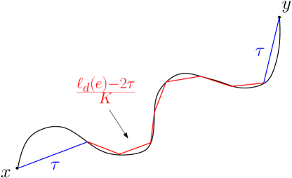
For the proof of this lemma, we follow the argument used in the main theorem in [Boi90]. The argument is almost exactly the same, but we reproduce it here for the reader’s convenience. First we will outline the proof. The first crucial element is the maximal lemma, Lemma 3.14 below, which gives an upper tail bound for the random variable . The next step is Lemma 3.15, which tells us that given any direction there is a in that direction at a far enough distance from the origin such that for a large constant which does not depend on
Now if the lemma is not true, then we must have a sequence such that
By extracting a subsequence, we can assume that We can then compare the distances and where with is an appropriate direction, is a large integer, and is such that are comparable. Combining everything we can conclude that yielding a contradiction.
First we claim that that the probability of being large is small. More precisely, we need to show the following “maximal lemma”:
Lemma 3.14.
For some fixed constant we have
Proof.
Let be the set of closed squares of side length with corners in For each pair of squares which share a side, we define the weight
For each , choose such that (if lies on the boundary of a square, we make an arbitrary choice). For , let
where the infimum runs over all paths of squares with and . By the triangle inequality,
Hence
Note that is stationary and ergodic by Lemma 3.1, and therefore so is Since has all moments up to by [DFG+20, Theorem 1.8] we can apply the maximal lemma in [Boi90] to see that
∎
Let be the event that
and write By Lemma 3.14 we know that
Following the notation in [Boi90], for , let
and for , define the partial cone
If is a function from the set of metrics on to let
Then as by the Birkhoff ergodic theorem. Therefore applying this to we get that almost surely, for each fixed and we have
as In particular, there is some such that for all we have
| (3.16) |
Lemma 3.15.
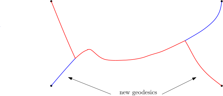
Suppose that is fixed. Suppose that Then if and for some large constant only depending on then there is a such that
Proof.
We have
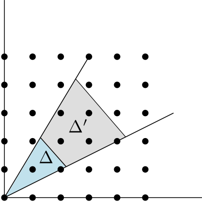
Let
and
(see Figure 1). Then
Hence
To prove the claim it is enough to have . By the above inequality, for this it suffices to have Explicit calculation of gives this inequality for large enough and ∎
Now if Lemma 3.14 is false, then we would have
If this is the case, then by compactness of the unit circle we can find a sequence with such that
| (3.17) |
for some Now we make a series of choices. Let be large enough so that
| (3.18) |
Also, take large enough so that there is a with and
| (3.19) |
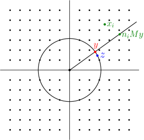
For , let be such that
| (3.20) |
and let be large enough so that for any
| (3.21) |
| (3.22) |
| (3.23) |
(which is possible by the ergodic theorem) and
| (3.24) |
(see Figure 2).
Lemma 3.16.
Let be fixed. Then for large enough and as in Lemma 3.15, there exists a such that
| (3.25) |
Proof.
By Lemma 3.15, there is a with such that
| (3.26) |
By repeated applications of the triangle inequality,
| (3.27) | |||||
∎
Recall from (3.17). We claim that
| (3.28) |
which will contradict (3.17). By the triangle inequality,
| (3.29) | |||||
Let be as in (3.26) taking Using (3.24) we obtain
| (3.30) | |||||
In the first line we used the fact that and so it is easy to see that
The first line follows. Plugging (3.29) and (3.30) into (3.25), we obtain
Now using (3.19),(3.21), and (3.22) we obtain hat for large enough we have
| (3.31) |
where in the last line we used (3.18). We also have by (3.20) and (3.23) that
| (3.32) | |||||
and
| (3.33) |
Finally, combining (3.32), (3.33), and (3.31), we obtain
which proves (3.28).
Now we are ready to prove Proposition 3.5.
Proof of Proposition 3.5.
Let be such that and Then we claim that for any fixed we have with probability tending to as that
Indeed, in Proposition 3.13 could be replaced with any other fixed point that is, almost surely we have that
By Lemma 3.2 and Lemma 3.1 we have that
| (3.34) |
as
Now fix and assume that is small enough that . By a union bound, it holds with probability tending to as that for each and all such that we have
Now suppose that Then there exists an such that
and
Therefore we obtain that
Similarly,
Noting that can be made smaller than any desired multiple of by making and small enough, we conclude the proof of Proposition 3.5. ∎
3.4 Controlling the total mass
Let be defined by
(which is well defined by Theorem 2.11 in [RV14]) Then by translation invariance, we have that for any positive integer
Therefore, by Markov’s inequality we have that for any small
as By Lemma 3.1, agrees in law with . By the Weyl scaling and LQG coordinate change properties of , we deduce that agrees in law with . Hence picking such that we obtain with probability tending to 1 as that
| (3.35) |
3.5 Making approximate with positive probability
We will need a couple of lemmas.
Lemma 3.17.
Let be a smooth function and let Let be as in (1.3). Suppose that ’s Fourier transform is compactly supported. Then there exists a with such that
Proof.
Since is compactly supported, its Fourier transform is well defined. Let denote the inverse Fourier transform. Define
We note that never vanishes, and hence is well defined and by the compact support of it is compactly supported. Therefore Also,
This completes the proof. ∎
The following lemma tells us that we can approximate uniformly by functions with compact Fourier support.
Lemma 3.18.
Let . Then there exists a countable family of smooth functions such that for any the function is compactly supported, and if in continuous in then there exists an element such that In particular, all elements in this net are Schwartz.
Proof.
Take to be any countable -net of smooth functions in . Let be a smooth function such that for and for Then for any and let Then has compactly supported Fourier transform, and as Now taking we have our desired net. ∎
Next, we need to construct functions such that the circle average at the unit circle can be arbitrarily large, but when convolved with is small.
Lemma 3.19.
Let and Then there is a smooth function such that
| (3.36) |
and
| (3.37) |
Proof.
The following lemma tells us that the circle average of at the unit circle is small if is small enough.
Lemma 3.20.
Let It holds with probability converging to as that
Proof.
We recall that is locally in for any by Proposition 2.7 in [She07]. Therefore in for any as Therefore as Since this completes the proof. ∎
We will also need the following lemma, which will also be used in Section 4
Lemma 3.21.
Let and Suppose that is an event such that Then there is a smooth, compactly supported function such that if and such that with positive probability,
Proof.
Let denote a family of functions compactly supported on that form a countable -net in (with the norm). Then
so there is some such that
This completes the proof. ∎
Let denote the norm for some large fixed Let denote the event in Lemma 3.20. Then by Lemma 3.21, there exists a smooth function such that
| (3.38) |
Suppose from now on that holds. By Lemma 3.17, there exists a smooth function such that
| (3.39) |
By Lemma 3.3 we can couple and in such a way that
Then we have that
where in the last line we used Lemma 3.3. Let and define where is given as in Lemma 3.19. Then we have by the triangle inequality that
| (3.40) | |||||
where in the last line we used Lemma 3.19. Now we claim that the event
| (3.41) |
holds with positive probability. Suppose that (3.41) holds for now. Then we have by the Cameron-Martin property of the GFF that it holds with positive probability that
Combining this with (3.40) we obtain that
with positive probability.
It remains to show that (3.41) holds with positive probability. Note that we already have with positive probability that we simultaneously have
and
Then
where in the last line we used (3.39). Now recall that by hypothesis. Hence by (3.38) we have
This implies that
Using Lemma 3.20 we obtain that (3.41) holds with positive probability.
Remark 3.22.
We note for future reference that the results in this section extend to the case where we have instead of by the exact same arguments. We could also replace by any bounded open set.
4 Approximating the Spherical Metric
Let be denote the spherical metric on the Riemann sphere . In this section we will prove that we can approximate the metric with the quantum sphere metric, where is any bounded continuous function on . This will be used in the proof of Theorem 1.5. Let be as in (1.9). We will focus on showing that with positive probability,
| (4.1) |
We will also show that can be forced to have small total mass. From now on our objective will be to prove (4.1). More precisely, the main result of this section is the following.
Theorem 4.1.
Let be a bounded continuous function on Let Then with positive probability, we have that (4.1) holds and simultaneously
| (4.2) |
We will get rid of the logarithmic singularities one at a time. We will first deal with the singularity at infinity, and then deal with the singularities at and
4.1 Interior and exterior control
Let
| (4.3) |
We note that far from the origin, behaves in the same way as More precisely, for ,
as Let be the circle average of at radius . Our main goal in this subsection is to show that several inequalities controlling the behaviour of both inside and outside an annulus.
We start with the following lemma, which tells us that with probability at least the exterior distances between points outside a large enough ball are small.
Lemma 4.2.
Let There exists a sufficiently large such that for all with probability at least we have that
| (4.4) |
Proof.
We will apply an inversion to map to . Applying LQG coordinate change, we have that and agree in law. Using that together with scaling, we obtain that
We have is finite, following the same proof as in Section 6.2 in [Gwy20]. Therefore tends to as with probability This completes the proof. ∎
We will now prove a series of lemmas that show that several conditions hold simultaneously with positive probability.
Recall the definition of as defined in (3.1).
Lemma 4.3.
Proof.
Lemma 4.4.
Proof.
Lemma 4.5.
Proof.
As in the proof of Lemma 4.2, we will apply an inversion to map to a small compact set. Applying LQG coordinate change, we have that for any Borel set
where Using that and have the same law and taking we obtain that and agree almost surely. Using as before that we obtain that the measure is locally finite. Thus taking to be large enough we will obtain that with probability at least . Combining this with Proposition 4.4 we conclude the result. ∎
Lemma 4.6.
Proof.
First, note that by covering with finitely many translations of we obtain by Proposition 3.6 that with probability going to as
| (4.10) |
Therefore if is fixed and is chosen to be small enough so that and (4.10) holds with probability at least we obtain the conclusion after combining this with Lemma 4.5. ∎
Proposition 4.7.
Proof.
This is a direct consequence of the Hölder continuity of the LQG metric, Theorem 1.7 in [DFG+20], together with (4.13) and Weyl scaling. Indeed, we have
with probability going to as Now one uses the Hölder continuity bound to conclude that (4.11) holds with probability at least One concludes the result after combining this with Lemma 4.6. ∎
Proposition 4.8.
Let Let be such that the conclusion of Lemma 4.3 holds with replaced by Let be as in Lemma 4.6. Let be as in Lemma 4.7. There exists a smooth, compactly supported function depending on with for such that with positive probability, we have that (4.4) holds with , (4.5), (4.6), (4.7), (4.8), (4.9), (4.11) hold, and simultaneously,
| (4.12) |
4.2 Bounds for the singularity at infinity
We will now use Proposition 4.8, and we will restrict to the case that (4.4), (4.5), (4.6), (4.12) hold, which we know is a positive probability event. Then
| (4.13) |
where we used (4.6) for the first term and (4.12) for the second. Recall that is a bounded continuous function. We let
Now we need a technical lemma.
Lemma 4.9.
If the conclusion of Proposition 4.8 holds, then we have that for small enough for any

Proof.
Let and let be a path of minimal -length between such that In particular,
where denotes the LQG length with respect to We claim that Indeed, suppose it is not contained in Let
(see Figure 3). Then by Proposition 3.5,
On the other hand, we have
| (4.15) |
and so if is large enough we obtain a contradiction by combining (4.2) and (4.15). To prove the lemma, we need to show that Suppose exits Let
Suppose that
| (4.16) |
Let be such that Then we have by Proposition 3.5
where in the last line we used (4.16). This implies that and thus
This completes the proof. ∎
We need the following technical lemma, which tells us that and are close when restricted to
Lemma 4.10.
Let Suppose that the conclusion of Proposition 4.8 holds. Then we have for small enough
| (4.17) |
Proof.
We have the decomposition
Using (4.12) and Lemma 4.4, we obtain
| (4.18) |
using that is bounded in and is compactly supported on and (4.4) (for ) we see that
| (4.19) |
We have controlled distances outside of and internal distances in within Now we will control distances in the annulus
Lemma 4.11.
Let and take as in Proposition 4.8. Then there exists a such that for all and any we have
Proof.
Now we can prove the following.
Theorem 4.12.
Proof.
First, shrinking if necessary note that we have the weaker version of (4.20),
by (4.19). Now to prove (4.20), suppose We define by
and we define similarly. Then using the triangle inequality,
By Proposition 4.7 we have that the first and second terms on the right are both at most For the third term, we use (4.4). This shows that
| (4.22) |
if Now it remains to prove the same for all Suppose that We let be defined in the following way. If then we let be such that
and if then we let We then have by the triangle inequality that
Then by (4.22) the last line is bounded by while by Lemma 4.11 the other two lines are bounded by This proves (4.20) for the general case.
4.3 Singularities at and
Let and let be a smooth function such that
and for all Let
and similarly let
Then on By Lemma 3.19 in [DFG+20] we have that the LQG metric with a log singularity of order less than induces the Euclidean topology, and thus
| (4.23) |
and similarly,
| (4.24) |
Again, using the inversion as in Lemma 4.2 together with LQG coordinate change for we obtain that
| (4.25) |
Now we will need the following lemma.
Lemma 4.13.
Let We have with positive probability that
| (4.26) |
and simultaneously
| (4.27) |
Proof.
We proceed in two steps. In the first one we show the -diameters of balls centered at the marked points are small. In the second step, we will be comparing distances in the and and then we use the fact that by Theorem 4.12 the metrics and are close. To compare the metrics and we decompose the geodesics into finitely many segments which are contained in and finitely many complementary segments. Then we use that in One proceeds similarly for the geodesics for The proof is longer than one might expect because of the need to define the decomposition of the geodesics.
Step 1: Bounding the diameters of neighborhoods of marked points.
We take
so that Using (4.23), (4.24), and (4.25) we know that there is a sufficiently small such that
and
Hence
| (4.28) |
Therefore
Taking small enough we obtain
| (4.29) |
Similarly, if is taken to be small enough then
| (4.30) |
In particular, if is small enough, then
| (4.31) |
Step 2: Comparing and Now by Theorem 4.12 applied to instead of we have that with positive probability, (4.27) holds and
| (4.32) |
We claim that
| (4.33) |
if is chosen to be small enough. In view of (4.32), it suffices to show that if then
First note that
since It remains to prove that
To prove this, let be a -length minimizing path between such that Let
We will now define a sequence of times to subdivide First we let
and define to be such that Now we define
Similarly we define
to be such that
to be such that and
(see Figure 4). Then by the triangle inequality, we have
Using (4.28) for and (4.31) for the second line we obtain that
| (4.34) |

Recall that and agree on and so if is chosen so that then we see that if are such that we have
Plugging this into (4.34) we obtain
This proves our claim (4.33). Now suppose that We define as follows: if we let be such that
If then we let We define similarly. Then we note that
Using (4.33) on the first term above we obtain
Now using (4.29) and (4.30), we see that are bounded by hence
Finally using the fact that for small enough,
we obtain that
This completes the proof. ∎
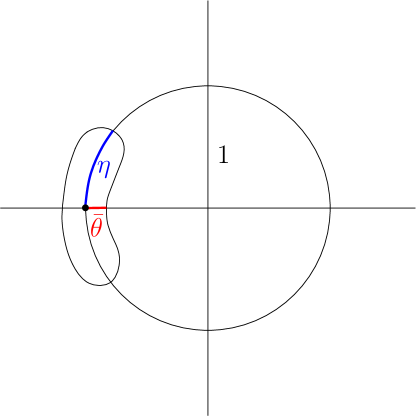
We want to extend the previous lemma to using the Cameron-Martin property of the GFF. However need not have finite Dirichlet energy. For this reason, note that for any there exists a compactly supported smooth function (which necessarily has finite Dirichlet energy) such that
| (4.35) |
Now, need not have average on and thus we still cannot use absolute continuity. We therefore add a bump function to to correct this. Let be defined by and for any let be defined by We define to be such that such that never changes sign, and such that if we let
| (4.36) |
we have
(see Figure 5). Note that because of scaling considerations, where constants do not depend on or
We claim that the addition of this bump function at does not affect the metric very much. More precisely, we have the following.
Lemma 4.14.
Let and let be as in (4.36). Suppose that Then for small enough and small we have with positive probability that
and simultaneously we have that
Proof.
For the proof, we will first show that if the -diameter of can be made small, then we are done since going around the ball does not modify distances very much. Then to prove that this diameter can be made small, we first reduce to showing the diameter of the support of is small. For this we show that the distance from any point in to is small. Then we show that the distance between a point inside to the boundary is small. Putting this information together tells us that the desired diameter is small.
We note that
Now we claim that are kept fixed, then
| (4.37) |
For now on we assume this and prove the lemma. We will show that if is fixed, then
From this, to show the lemma it suffices to note that
and then combining these two facts we obtain the result.
To prove (4.37) we split into two cases.
Case 1: In this case, the sign of the bump implies that for any
Since
we obtain (4.37).
Case 2: This case is similar to the previous case. In this case, the sign of the bump implies that for any
and so we obtain from (4.35) that
Suppose that Let be a -length minimizing path between such that Then if we have that
and thus in this case we would be done. If not, let
Then again by the triangle inequality we have
By (4.37) the last term is bounded by Using again the support of we obtain together with (4.35) that
Now it remains to look at the case Noting that
we see that
Now we prove (4.37).
Proof of (4.37).
First we claim that for small enough we have that
| (4.38) |
Assume (4.38) is proven. Suppose that Taking a path between and of Euclidean length at most such that we see that
If is small enough, this last expression can be made to be at most Now in the case we let be such that and Then we have by the triangle inequality that
If we take a path such that between and we see that
and so again for small enough this is at most This proves the claim (4.37). It remains to show (4.38). Let denote the horizontal path from to Then the image under of this path is of length at most Therefore
as This completes the proof. ∎
∎
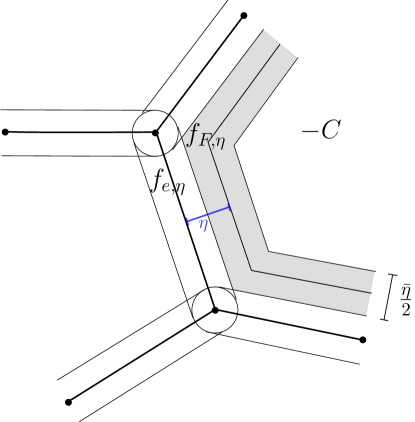
5 Increasing measure without changing metric
Let be a bounded continuous function. By the results of the previous section, with positive probability we have
and also
If we are able to change the measure without changing the metric very much, we can then use the results from Section 4 and prove Theorem 1.5 in the case of any Riemannian metric of the form together with any finite measure on Therefore the set of metric measure spaces that can be approximated by Liouville quantum spheres with positive probability and the closure of Riemannian metrics on the sphere are the same. Now by the results in the Appendix, this proves Theorem 1.5.
5.1 Proof of Theorem 1.5
The idea will be to add bump functions to the Gaussian free field which will locally add mass at the centers of these bumps, but will not affect distances very much since geodesics can go around these bumps. To this end, suppose that is a set of points in and suppose that are positive weights. Let denote the event that the conclusion of Theorem 4.1 holds, which is a positive probability event. Let be large positive integers, and let be small. For each we will subdivide the square into four sets with defined as follows:
(see Figure 6 for a picture). The idea of considering sets of these is taken from the proof of Lemma 11.10 in [BG22].
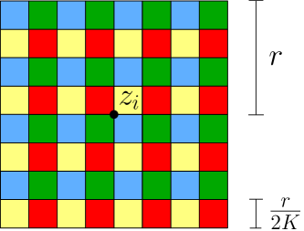
Let be a small constant. Since induces the Euclidean topology, the maximum size of the squares go to as By this and the pigeonhole principle, we can take deterministic such that with positive probability, holds, and simultaneously
| (5.1) |
for all and
| (5.2) |
To simplify notation, we let
| (5.3) |
Now we will “fix” the masses around each point We have the following lemma.
Lemma 5.1.
Proof.
Note that the event that , (5.1), (5.2) hold simultaneously is an event of positive probability by construction. The result follows as a direct consequence of the pigeonhole principle. To select we note that a non-deterministic satisfying (5.4) exists with probability and so there exists a deterministic satisfying (5.4) simultaneously with the conditions , (5.1), and (5.2). Finally, note that the probability of (5.5) holds with probability going to as so we can also assume this holds simultaneously. This completes the proof. ∎
Therefore for any there exist deterministic constants such that with positive probability, (5.1), (5.2), (5.4) hold, and simultaneously
| (5.6) |
We will define our bump functions now. For any we let be defined as follows:
| (5.7) |
We additionally impose that if and that if but (see Figure 7 for a picture of ).

Now we define
| (5.8) |
We will prove the following proposition.
Proposition 5.2.
Proof.
First we note that we can reduce to the case that Indeed, let be smooth functions such that
and Then by the triangle inequality we have
where in the last line we used the fact that by Theorem 4.1. Therefore shrinking if necessary, it suffices to prove the proposition for the case when We then have a single point with its weight Without loss of generality, suppose that Since we have a single point mass, we will drop the subscript on We split into three regions,
Splitting into these domains we obtain
Note that
where we used the fact that if Using (5.4), we obtain that
| (5.9) |
Similarly, we have with probability that
| (5.10) |
| (5.11) |
Note that
| (5.12) |
by (5.6) and the fact that is continuous. Therefore taking to be small enough we obtain we obtain
| (5.13) |
∎
Now we claim the metric doesn’t change much when adding .
Proposition 5.3.
Let For large enough and small enough we have that with positive probability that the conclusion of Lemma 5.1 holds, and simultaneously for all
We will prove Proposition 5.3 in Subsection 5.2. We will prove now Theorem 1.5 assuming Proposition 5.3.
Proof of Theorem 1.5 assuming Proposition 5.3.
Suppose that is a Riemannian metric in its isothermal form, and let be a probability measure on We will show Theorem 1.5 for this metric and measure. Let be as in (5.8). We now introduce a finite set of functions to which we will apply Proposition 5.3. Let be a triangulation of Let be the set of faces of the triangulation with the set of stereographic projections onto Suppose that has been chosen such that for any For each finite subset let be a smooth function such that
For any there exist points and weights such that for any we have
| (5.14) |
Then applying Proposition 5.2 to for every taking to be small enough we obtain that with positive probability for any we have
| (5.15) |
(4.1) holds and simultaneously
Therefore using (5.14) we obtain
where in the last inequality we used (5.14) and (5.15). Again, for large enough and small enough applying Proposition 5.3 we obtain that for all we have
| (5.16) |
Recall that we assumed that Thus using the Cameron-Martin property applied to we obtain that for any we have with positive probability that
| (5.17) |
| (5.18) |
and simultaneously
To pass to a statement about measures of sets, suppose that is a measurable set, and let such that and Then
which implies that
| (5.19) |
This completes the proof.
5.2 Proof of Proposition 5.3
The first ingredient we need is the following lemma.
Lemma 5.5.
Assume that the events in the conclusion of Lemma 5.1 hold. Let Then for large enough we have for all we have that
For now we will assume the validity of this lemma and prove Proposition 5.3.
Suppose and let be a -distance minimizing geodesic between We claim that
Indeed, by applying a procedure similar to the proof or Lemma 4.13, there exist intervals such that and additionally, for every for some Then
This proves the claim. Now note that
Now applying Lemma 5.5 we conclude the upper bound for The lower bound can be obtained in the exact same way interchanging the metrics and This completes the proof of Proposition 5.3.
For the proof of Lemma 5.5, we will need the following lemma.
Lemma 5.6.
Assume that the events in the conclusion of Lemma 5.1 hold. Suppose that for some Let Then for large enough depending on we have
Proof.
By (5.2), we have that
Therefore if is any path between and of Euclidean length at most we note that
Now choosing large enough so that
we conclude. ∎
Now we will prove Lemma 5.5.
Proof of Lemma 5.5.
Now suppose that Then by the triangle inequality,
where for any point we define
and where is defined to be such that if and defined as otherwise (see Figures 9 and 9).


By Lemma 5.6, for small enough we have that Additionally, we note that by taking a path between not intersecting of -length at most
and so for a small enough choice of and large enough so that we conclude that
∎
Appendix A Appendix
In this appendix we show that any length metric space homeomorphic to the sphere can be approximated by Riemannian metrics on the sphere. More precisely, we will prove the following.
Theorem A.1.
Let be a length metric on which induces the same topology as the standard spherical metric Let Then there exists a bounded continuous function such that
Recall that denotes the Euclidean distance on If we identify the Riemann sphere , then the metric is uniformly continuous with respect to the Euclidean metric on and satisfies . Let We will then show that there exists a bounded continuous function such that
We will first construct a graph embedded into with weights on the edges, with the property that the weighted graph distance between any two vertices is close to their -distance. The edges of the graph will be approximations of -geodesics. After this, we choose an appropriate function such that approximates this graph metric. Finally, we put these together and bound distances between any pair of points in
We start by constructing the graph approximation of . Let be large enough so that
| (A.1) |
Note that this exists since induces the same topology as Now let and subdivide into squares , of side length Again, since and induce the same topology, we can take large enough so that
| (A.2) |
Take a large integer and further subdivide each into squares of side We label these squares as in such a way that
Let denote the graph consisting of the vertices and with edges being -length minimizing paths between all pairs of vertices. The geodesics in this set can intersect each other, possibly infinitely many times.
Our next step is to replace these geodesics by other -length minimizing geodesics such that any pair intersects at either the endpoints, or at a single curve segment. More precisely:
Lemma A.2.
Suppose that is a finite set of -geodesics between pairs of points in Then there exists another set of geodesics between the same pairs of points such that each the intersection of each pair of geodesics in is either a common segment or a single point.
Proof.
We first consider a single pair of geodesics, and note that we can replace these two geodesics so that they intersect at either a single point or in an interval. Indeed, suppose are geodesics between and and that they intersect at at least two points. Let
and let such that and Recall that since intersect at least twice, Since is a length minimizing geodesic, it is also length minimizing when restricting to an interval. Therefore is a length minimizing path between Thus we can replace by where denotes concatenation. This procedure lets us replace two geodesics with multiple intersection points with geodesics whose intersection is a single interval (see Figures 11 and 11). Suppose we number the geodesics in arbitrarily, so that the geodesics are the set for some large We will inductively apply this procedure to to get rid of all intersections that are not at endpoints or single segments. First we apply the procedure to and to replace them with geodesics intersecting at their endpoints. Now suppose that we have replaced with geodesics intersecting only at endpoints, where Let
Now let be such that Then we define
Suppose we have defined and Then define
let such that and finally let
Note that the intervals are disjoint. Now applying the above procedure we can replace in the intervals by the corresponding segments on thus removing multiple intersections, leaving us with only intersection at the endpoints. This completes the proof. ∎
By applying the above lemma to the geodesics of we end up with a graph whose vertices are points of and whose edges are geodesics between the vertices and intersect either at points or single curve segments. We also define the faces of to be the connected components of the complement of the union of all edges. To make things easier, we make the faces be closed sets.
Now let be small. Note that for large enough any edge in the graph between two vertices in is contained in This comes from the uniform continuity of with respect to In particular, by (A.2), we have that for any face we have
| (A.3) |
Now at the points where any pair of geodesics merge, add a vertex to the graph, and divide the edges accordingly to obtain a new graph Note that is such that all faces are of -diameter at most
We will now replace each geodesic with a piecewise linear approximation. To ensure that these piecwise linear approximations do not intersect, we have a larger step size near each vertex than on each edge far away from vertices. Let be small, and let be a large integer. First we subdivide each geodesic edge of into three segments: two at the endpoints of -length and a middle segment of length We further subdivide the middle segment into segments of length (see Figure 12). Let the points where these line segments meet be new vertices. We have now obtained a new graph If is chosen large enough so that
and it is easy to see that the new edges do not intersect. Let
and for any
We will now assign weights to all edges of this graph. If denotes an edge on the graph with as its endpoints, then let be the corresponding weights and define to be the weighted graph distance on Let denote this weighted graph we have constructed. Let Then taking large enough and recalling that is uniformly continuous with respect to we see that is a weighted graph whose vertices form a -net, whose edges are straight line segments, and whose edges only intersect at endpoints.
Note that
| (A.4) |
for large enough Indeed, let be such that the path formed by the edges is the path of least length between Then since
we see that
For the reverse inequality one uses the fact that the set of vertices of is an -net together with the fact that the edges of are -geodesics.
Let be the set of faces of Let For each face let
Also let be a large constant to be chosen later. Let be large and be small. Then define a smooth function such that
where is a large constant to be chosen later, denotes the Euclidean distance, and such that
if and
if We also define for each edge a smooth function such that
and if See Figure 13 for a picture of Define
We claim that
| (A.5) |
Note that (A.5) together with (A.1) implies Theorem A.1. To prove (A.5) we will need a couple of lemmas:
Lemma A.3.
Let be adjacent vertices. Let be as above. For small enough we have
where denotes the number of edges in
This lemma tells us that for adjacent vertices, the distances and are very close. Next we need a lemma that constrains geodesics between points close to edges of to also be close to edges of
Lemma A.4.
Let Suppose that and let be a -distance minimizing path between them. Then there exists a constant only depending on such that if then
We will proceed by proving upper and lower bounds for in the case that first in subsection A.1, and then in subsection A.2 we prove upper and lower bounds in the case that where is a face in
A.1 Comparing metrics: the edge case
The main results in this subsection are the following.
Lemma A.5.
Suppose that are vertices on the graph Then we have the inequality
| (A.6) |
Lemma A.6.
Suppose that are vertices in Then we have the bound
| (A.7) |
First we prove Lemma A.5.
Proof of Lemma A.5.
Let be a path consisting of edges on connecting with minimal -length. Let be the vertices that this path passes through in order, so that and are adjacent, and Then we have by the triangle inequality that
Now using Lemma A.3 we obtain that
Now note that given the choice of weights on for vertices This proves Lemma A.5. ∎
We will now prove Lemma A.6.
Let be a -length minimizing path between such that Then we know by Lemma A.4 that We must prove that for any vertices
For each edge on and we let Let be the minimal set of edges such that
is connected, and contains Let be such that and are adjacent, the edge between is in and where denotes the edge between if are adjacent vertices in (see Figure 14).

Now we need the following lemma.
Lemma A.7.
We have that
| (A.8) |
Proof.
To show this, let be an -length minimizing path between Recall that by Lemma A.4 we know that is contained in Suppose that is an edge and for small enough and is such that Then if is at -distance at least from the endpoints of we have (this comes directly from the definition of ). We will define the sequences of times such that
and
so that
Then using that for any edges we have that as it suffices to prove that
where denotes the number of edges in the graph We have
where is such that if we have
Then for small enough
since
Noting that
we obtain Lemma A.7. ∎
Now we will prove Lemma A.6.
Proof of Lemma A.6.
By the triangle inequality, we have that
| (A.9) |
Note that tends to as Letting be small enough we obtain that since if and are small enough we know that
and similarly
Combining this with (A.9) we obtain that
Similarly we obtain by the triangle inequality that
Combining this with Lemma A.7 we conclude the proof of Lemma A.6. ∎
A.2 Comparing metrics: the interior case
The main result of this subsection is the following.
Lemma A.8.
Suppose that is a face in and that Then
| (A.10) |
Let us assume the validity of Lemma A.8 for now. Suppose that First we note that the maximal diameter of the a face in is smaller than the maximal diameter of a face for Indeed, note that the diameter of a face in coincides with the diameter of its convex hull, which in turn bounds from above the diameter of the faces of Hence for small enough we have by (A.3) that
Putting this together with Lemma A.8 we would obtain
| (A.11) |
After this, it remains to prove the following.
Lemma A.9.
For any pair of points we have
Proof.
Assume first that Let be vertices such that are minimized (note it is possible for ). Then using the triangle inequality, we have that
Now using Lemma A.5 and A.6 we conclude the result in this case. Now if then let be such that the -distance is minimized. Then using the triangle inequality we obtain
Using that the result holds for together with (A.1) we obtain the result for general ∎
To prove Lemma A.8 we split into three cases.
Case 1: In this case, considering any curve between contained in of Euclidean length we see that by the definition of
and so taking to be large enough (depending on ) we obtain that
Case 2: and Note that if which can be guaranteed by taking we obtain that
Now using the triangle inequality we obtain that
Case 3: and This follows from Case 2 and the triangle inequality.
This completes the proof.
A.3 Proof of Theorem A.1
A.4 Proofs of Lemmas A.3 and A.4
Define the constant
Note that can be made to be arbitrarily small by (A.3), so we can assume that
| (A.12) |
Before we prove Lemma A.4, we will need the following lemma.
Lemma A.10.
There is a choice of such that the following holds. Suppose is a face in Suppose that and let be a path between contained in Assume that
Then there exists a path between contained in such that
Proof.
We let
Then we have that
Recall that for such that Therefore
Let be vertices in such that and are minimized. Let be a length minimizing -geodesic between Taking
(which is possible by (A.12)) yields
This completes the proof. ∎
Now we will prove Lemma A.4.
Proof of Lemma A.4.
Suppose that and is a -distance minimizing path between them with The idea of the proof is that if exits then the parts of that go between and will have large -length. We claim that there is no face such that By contradiction, suppose such an exists. Then by Lemma A.10 we have that there exists a path between such that
Therefore
This contradicts the fact that is -length minimizing.
Thus This completes the proof. ∎
Proof of Lemma A.3.
Suppose that are adjacent vertices. Let be the edge between and let Taking the path we see that
Then it remains to show the other inequality. Suppose that is a -distance minimizing path between Note that by Lemma A.4, where again we recall that denotes the edge between We claim that
Let be the projection of the path onto the edge that is for each let be the unique point such that It is easy to check that is also continuous. For , let denote the -ball of radius centered at and let be defined by
are used to split off the endpoints of the edge. This way, is smaller at the projection onto the edge if away from the endpoints. We thus have for small enough that
This completes the proof. ∎
References
- [AA21] L. Addario-Berry and M. Albenque. Convergence of odd-angulations via symmetrization of labeled trees. Annales Henri Lebesgue, 4:653–683, 2021, 1904.04786.
- [ABA17] L. Addario-Berry and M. Albenque. The scaling limit of random simple triangulations and random simple quadrangulations. Ann. Probab., 45(5):2767–2825, 2017, 1306.5227. MR3706731
- [AHS17] J. Aru, Y. Huang, and X. Sun. Two perspectives of the 2D unit area quantum sphere and their equivalence. Comm. Math. Phys., 356(1):261–283, 2017, 1512.06190. MR3694028
- [BBI01] D. Burago, Y. Burago, and S. Ivanov. A course in metric geometry, volume 33 of Graduate Studies in Mathematics. American Mathematical Society, Providence, RI, 2001. MR1835418
- [Ber17] N. Berestycki. An elementary approach to Gaussian multiplicative chaos. Electron. Commun. Probab., 22:Paper No. 27, 12, 2017, 1506.09113. MR3652040
- [BG22] A. Bou-Rabee and E. Gwynne. Harmonic balls in Liouville quantum gravity. ArXiv e-prints, August 2022, 2208.11795.
- [BJM14] J. Bettinelli, E. Jacob, and G. Miermont. The scaling limit of uniform random plane maps, via the Ambjørn-Budd bijection. Electron. J. Probab., 19:no. 74, 16, 2014, 1312.5842. MR3256874
- [Boi90] D. Boivin. First passage percolation: the stationary case. Probability theory and related fields, 86(4):491–499, 1990.
- [BP] N. Berestycki and E. Powell. Gaussian free field, Liouville quantum gravity, and Gaussian multiplicative chaos. Available at https://homepage.univie.ac.at/nathanael.berestycki/Articles/master.pdf.
- [BRG22] A. Bou-Rabee and E. Gwynne. Harmonic balls in liouville quantum gravity. arXiv preprint arXiv:2208.11795, 2022.
- [DDDF20] J. Ding, J. Dubédat, A. Dunlap, and H. Falconet. Tightness of Liouville first passage percolation for . Publ. Math. Inst. Hautes Études Sci., 132:353–403, 2020, 1904.08021. MR4179836
- [DDG21] J. Ding, J. Dubedat, and E. Gwynne. Introduction to the Liouville quantum gravity metric. ArXiv e-prints, September 2021, 2109.01252.
- [DF20] J. Dubédat and H. Falconet. Liouville metric of star-scale invariant fields: tails and Weyl scaling. Probab. Theory Related Fields, 176(1-2):293–352, 2020, 1809.02607. MR4055191
- [DFG+20] J. Dubédat, H. Falconet, E. Gwynne, J. Pfeffer, and X. Sun. Weak LQG metrics and Liouville first passage percolation. Probab. Theory Related Fields, 178(1-2):369–436, 2020, 1905.00380. MR4146541
- [DG18] J. Ding and E. Gwynne. The fractal dimension of Liouville quantum gravity: universality, monotonicity, and bounds. Communications in Mathematical Physics, 374:1877–1934, 2018, 1807.01072.
- [DG19] J. Ding and S. Goswami. Upper bounds on Liouville first-passage percolation and Watabiki’s prediction. Comm. Pure Appl. Math., 72(11):2331–2384, 2019, 1610.09998. MR4011862
- [DKRV16] F. David, A. Kupiainen, R. Rhodes, and V. Vargas. Liouville quantum gravity on the Riemann sphere. Comm. Math. Phys., 342(3):869–907, 2016, 1410.7318. MR3465434
- [DMS21] B. Duplantier, J. Miller, and S. Sheffield. Liouville quantum gravity as a mating of trees. Astérisque, 427(427):viii+257, 2021, 1409.7055. MR4340069
- [DRV16] F. David, R. Rhodes, and V. Vargas. Liouville quantum gravity on complex tori. J. Math. Phys., 57(2):022302, 25, 2016, 1504.00625. MR3450564
- [DRZ17] J. Ding, R. Roy, and O. Zeitouni. Convergence of the centered maximum of log-correlated gaussian fields. The Annals of Probability, 45(6A):3886–3928, 2017.
- [DS11] B. Duplantier and S. Sheffield. Liouville quantum gravity and KPZ. Invent. Math., 185(2):333–393, 2011, 1206.0212. MR2819163 (2012f:81251)
- [DZZ19] J. Ding, O. Zeitouni, and F. Zhang. Heat kernel for Liouville Brownian motion and Liouville graph distance. Comm. Math. Phys., 371(2):561–618, 2019, 1807.00422. MR4019914
- [GM20a] E. Gwynne and J. Miller. Confluence of geodesics in Liouville quantum gravity for . Ann. Probab., 48(4):1861–1901, 2020, 1905.00381. MR4124527
- [GM20b] E. Gwynne and J. Miller. Local metrics of the Gaussian free field. Ann. Inst. Fourier (Grenoble), 70(5):2049–2075, 2020, 1905.00379. MR4245606
- [GM21a] E. Gwynne and J. Miller. Existence and uniqueness of the liouville quantum gravity metric for . Inventiones mathematicae, 223(1):213–333, 2021.
- [GM21b] E. Gwynne and J. Miller. Existence and uniqueness of the Liouville quantum gravity metric for . Invent. Math., 223(1):213–333, 2021, 1905.00383. MR4199443
- [GP19] E. Gwynne and J. Pfeffer. KPZ formulas for the Liouville quantum gravity metric. Transactions of the American Mathematical Society, to appear, 2019.
- [GRV19] C. Guillarmou, R. Rhodes, and V. Vargas. Polyakov’s formulation of bosonic string theory. Publ. Math. Inst. Hautes Études Sci., 130:111–185, 2019, 1607.08467. MR4028515
- [GS22] E. Gwynne and J. Sung. The Minkowski content measure of the Liouville quantum gravity metric. In preparation, 2022.
- [Gwy20] E. Gwynne. The dimension of the boundary of a liouville quantum gravity metric ball. Communications in Mathematical Physics, 378:625–689, 2020.
- [Kah85] J.-P. Kahane. Sur le chaos multiplicatif. Ann. Sci. Math. Québec, 9(2):105–150, 1985. MR829798 (88h:60099a)
- [Kin68] J. F. Kingman. The ergodic theory of subadditive stochastic processes. Journal of the Royal Statistical Society: Series B (Methodological), 30(3):499–510, 1968.
- [Le 13] J.-F. Le Gall. Uniqueness and universality of the Brownian map. Ann. Probab., 41(4):2880–2960, 2013, 1105.4842. MR3112934
- [LG14] J.-F. Le Gall. Random geometry on the sphere. In Proceedings of the International Congress of Mathematicians—Seoul 2014. Vol. 1, pages 421–442. Kyung Moon Sa, Seoul, 2014, 1403.7943. MR3728478
- [Mar22] C. Marzouk. On scaling limits of random trees and maps with a prescribed degree sequence. Ann. H. Lebesgue, 5:317–386, 2022, 1903.06138. MR4443293
- [Mie13] G. Miermont. The Brownian map is the scaling limit of uniform random plane quadrangulations. Acta Math., 210(2):319–401, 2013, 1104.1606. MR3070569
- [MS16] J. Miller and S. Sheffield. Liouville quantum gravity and the brownian map iii: the conformal structure is determined. arXiv preprint arXiv:1608.05391, 2016.
- [MS17] J. Miller and S. Sheffield. Imaginary geometry IV: interior rays, whole-plane reversibility, and space-filling trees. Probab. Theory Related Fields, 169(3-4):729–869, 2017, 1302.4738. MR3719057
- [MS20] J. Miller and S. Sheffield. Liouville quantum gravity and the brownian map i: the metric. Inventiones mathematicae, 219(1):75–152, 2020.
- [MS21] J. Miller and S. Sheffield. Liouville quantum gravity and the brownian map ii: geodesics and continuity of the embedding. The Annals of Probability, 49(6):2732–2829, 2021.
- [MW17] J. Miller and H. Wu. Intersections of SLE Paths: the double and cut point dimension of SLE. Probab. Theory Related Fields, 167(1-2):45–105, 2017, 1303.4725. MR3602842
- [Pol81] A. M. Polyakov. Quantum geometry of bosonic strings. Phys. Lett. B, 103(3):207–210, 1981. MR623209 (84h:81093a)
- [Rem18] G. Remy. Liouville quantum gravity on the annulus. J. Math. Phys., 59(8):082303, 26, 2018, 1711.06547. MR3843631
- [RV14] R. Rhodes and V. Vargas. Gaussian multiplicative chaos and applications: A review. Probab. Surv., 11:315–392, 2014, 1305.6221. MR3274356
- [She07] S. Sheffield. Gaussian free fields for mathematicians. Probab. Theory Related Fields, 139(3-4):521–541, 2007, math/0312099. MR2322706 (2008d:60120)
- [Shi99] T. Shioya. The limit spaces of two-dimensional manifolds with uniformly bounded integral curvature. Transactions of the American Mathematical Society, 351(5):1765–1801, 1999.
- [SW16] S. Sheffield and M. Wang. Field-measure correspondence in Liouville quantum gravity almost surely commutes with all conformal maps simultaneously. ArXiv e-prints, May 2016, 1605.06171.
- [Var17] V. Vargas. Lecture notes on Liouville theory and the DOZZ formula. ArXiv e-prints, Dec 2017, 1712.00829.
- [WP20] W. Werner and E. Powell. Lecture notes on the Gaussian Free Field. ArXiv e-prints, April 2020, 2004.04720.