Minimizing $f$-Divergences by Interpolating Velocity Fields

Abstract

Many machine learning problems can be formulated as approximating a target distribution using a particle distribution by minimizing a statistical discrepancy. Wasserstein Gradient Flow can be employed to move particles along a path that minimizes the $f$-divergence between the target and particle distributions. To perform such movements we need to calculate the corresponding velocity fields which include a density ratio function between these two distributions. While previous works estimated the density ratio function first and then differentiated the estimated ratio, this approach may suffer from overfitting, which leads to a less accurate estimate. Inspired by non-parametric curve fitting, we directly estimate these velocity fields using interpolation. We prove that our method is asymptotically consistent under mild conditions. We validate the effectiveness using novel applications on domain adaptation and missing data imputation.

1 Introduction

Many machine learning problems can be formulated as minimizing a statistical divergence between distributions, e.g., Variational Inference (Blei et al., 2017), Generative Modeling (Nowozin et al., 2016; Yi et al., 2023), and Domain Adaptation (Courty et al., 2017a; Yu et al., 2021). Among many divergence minimization techniques, Particle based Gradient Descent reduces the divergence between a set of particles (which define a distribution) and the target distribution. It achieves that by iteratively moving particles according to an update rule. One such algorithm is Stein Variational Gradient Descent (SVGD) (Liu and Wang, 2016; Liu, 2017). It minimizes the Kullback-Leibler (KL) divergence by using the steepest descent algorithm. While it has achieved promising results in Bayesian inference, in some other applications, for example, in domain adaptation and generative model training, we only have samples from the target dataset. SVGD requires an unnormalized target density function, thus cannot be straightforwardly applied to minimize the $f$-divergence in these applications.

Wasserstein Gradient Flows (WGF) describe the evolution of marginal measures $q_{t}$ along the steepest descent direction of a functional objective in Wasserstein geometry where $x_{t}\sim q_{t}$ follows a probability flow ODE. It can also be used to minimize an $f$-divergence between a particle distribution and the target distribution. Particularly, such WGFs characterize the following ODE (Yi et al., 2023; Gao et al., 2019)

$$\mathrm{d}{\boldsymbol{x}}_{t}=\nabla(h\circ r_{t})({\boldsymbol{x}}_{t})\mathrm{d}t,~{}~{}~{}t\in[0,\infty).$$

Here $r_{t}:=\frac{p}{q_{t}}$ is the ratio between the target density $p$ and particle density $q_{t}$ at time $t$, and $h$ is a known function which depends on the $f$-divergence. The gradient operator $\nabla$ computes the gradient of the composite function $h\circ r_{t}$. If we knew $r_{t}$, simulating the above ODE would be straightforward by using a discrete time Euler method. However, the main challenge is that we do not know the ratio $r_{t}$ in practice. In fact, in the context we consider, we know neither the particle nor target density which constitutes $r_{t}$.

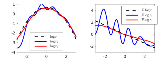
Figure 1: Estimating a log density ratio $\log r$ using a flexible model (RBF kernel) leads to a severely overfitted estimate ($\log r_{1}$). The overfitting consequently causes huge fluctuations in the derivative $(\log r_{1})^{\prime}$. Our proposed method provides a much more stable estimate $\log r_{2}$ and a more accurate estimate of $(\log r_{2})^{\prime}$.

To overcome this issue, some recent works (Gao et al., 2019; Ansari et al., 2021; Simons et al., 2021) first obtain an estimate $\hat{r}_{t}$ using density ratio estimator (Sugiyama et al., 2012), then differentiate $h\circ\hat{r}_{t}$ to obtain $\nabla(h\circ\hat{r}_{t})({\boldsymbol{x}}_{t})$. However, like other estimation tasks, density ratio estimation can be prone to overfitting. The risk of overfitting is further exacerbated when employing flexible models such as kernel models or neural networks. Overfitting can be disastrous for gradient estimation: A wiggly fit of $r_{t}$ will cause huge fluctuations in gradient estimation (see the blue fit in Figure 1). Moreover, density ratio estimation lacks the inductive bias for the density ratio gradient estimation. In other words, density ratio estimation doesn’t make any direct assumption on how the ratio function changes across different inputs, and thus is unlikely to perform well on the gradient estimation task.

In this paper, we directly approximate the velocity fields induced by WGF, i.e., $\nabla(h\circ r_{t})({\boldsymbol{x}}_{t})$. We show that the backward KL velocity field, where $h=\log$, can be effectively estimated using Nadaraya Watson (NW) interpolation if we know $\nabla\log p$, and this estimator is closely related to SVGD. We prove this estimator is an asymptotically consistent estimator of $\nabla\log r_{t}({\boldsymbol{x}}_{t})$, as the kernel bandwidth approaches to zero. This finding motivates us to propose a more general linear interpolation method to approximate $\nabla(h\circ r_{t})({\boldsymbol{x}}_{t})$ for any general $h$ functions using only samples from $p$ and $q_{t}$. Our estimators are based on the idea that, within the neighbourhood of a given point, the best linear approximation of $h\circ r_{t}$ has a slope $\nabla(h\circ r_{t})$. Under mild conditions, we show that our estimators are also asymptotically consistent for estimating $\nabla(h\circ r_{t})({\boldsymbol{x}}_{t})$ and achieve the optimal non-parametric regression rate. Finally, equipped with our proposed gradient estimator, we test WGF on two novel applications: domain adaptation and missing data imputation and achieve state-of-the-art performance.

2 Background

Notation: $\mathbb{R}^{d}$ is the $d$-dimensional real domain. Vectors are lowercase bold letters, e.g., ${\boldsymbol{x}}:=[x_{1},\ldots,x_{d}]^{\top}$. ${\boldsymbol{x}}_{-j}$ is a subvector of ${\boldsymbol{x}}$ obtained by excluding the $j$-th dimension. Matrices are uppercase bold letters, e.g., ${\boldsymbol{X}},{\boldsymbol{Y}}$. $f\circ g$ is the composite function $f(g(\cdot))$. $f^{\prime}$ is the derivative of a univariate function. $\partial_{i}f$ means the partial derivative with respect to the $i$-th input of $f$ and $\nabla f:=[\partial_{1}f,\partial_{2}f,\cdots,\partial_{d}f]^{\top}$. $\nabla^{\top}f$ represents its transpose. $\nabla_{\boldsymbol{x}}f({\boldsymbol{x}},{\boldsymbol{y}})$ represents the gradient of $f$ with respect to the input ${\boldsymbol{x}}$. $\nabla{\boldsymbol{f}}\in\mathbb{R}^{d\times m}$ represents the Jacobian of a vector-valued function ${\boldsymbol{f}}:\mathbb{R}^{m}\to\mathbb{R}^{d}$. $\partial^{2}_{i}f$ means the second-order partial derivative with respect to the $i$-th input of $f$. $\nabla^{2}f$ is the Hessian of $f$. $\lambda_{\min}\left[{\boldsymbol{X}}\right]$ represents the smallest eigenvalue of a matrix ${\boldsymbol{X}}$. $a\vee b$ is the greater value between two scalars $a$ and $b$. $\mathcal{P}(\mathbb{R}^{d})$ is the space of probability measures defined on $\mathbb{R}^{d}$ equipped with Wasserstein-2 metric or Wasserstein space for short. $\hat{\mathbb{E}}[\cdot]$ is the sample approximation of an expectation $\mathbb{E}[\cdot]$.

We begin by introducing WGF of $f$-divergence, an efficient way of minimizing $f$-divergence between the particle and target distribution.

2.1 Wasserstein Gradient Flows of $f$-divergence

In general terms, a Wasserstein Gradient Flow is a curve in probability space (Ambrosio et al., 2005). By moving a probability measure along this curve, a functional objective (such as a statistical divergence) is reduced. In this work, we focus solely on using $f$-divergences as the functional objective. Let $q_{t}:\mathbb{R}_{+}\to\mathcal{P}(\mathbb{R}^{d})$ be a curve in Wasserstein space. Consider an $f$-divergence defined by $D_{f}[p,q_{t}]:=\int q_{t}({\boldsymbol{x}})f(r_{t}({\boldsymbol{x}}))\mathrm{d}{\boldsymbol{x}}$, where $r_{t}:=\frac{p}{q_{t}}$. $f$ is a twice differentiable convex function with $f(1)=0$.

Theorem 2.1 (Corollary 3.3 in (Yi et al., 2023)).

The Wasserstein gradient flow of $D_{f}[p,q_{t}]$ characterizes the particle evolution via the ODE:

$$\mathrm{d}{\boldsymbol{x}}_{t} =\nabla(h\circ r_{t})({\boldsymbol{x}}_{t})\mathrm{d}t,~{}h(r_{t})=r_{t}f^{\prime}(r_{t})-f(r_{t}).$$

Simply speaking, particles evolve in Euclidean space according to the above ODE moves the corresponding $q_{t}$ along a curve where $D_{f}[p,q_{t}]$ always decreases with time.

Theorem 2.1 establishes a relationship between $f$ and a function $h:\mathbb{R}_{+}\mapsto\mathbb{R}$. The gradient field of $h\circ r_{t}$ over time as $t\to\infty$ is referred to as the WGF velocity field. Similar theorems on backward $f$-divergences have been discussed in (Gao et al., 2019; Ansari et al., 2021). Some frequently used $f$-divergence and their corresponding $h$ functions are listed in Table 1. Specifically, for the backward KL divergence we have $\nabla(h\circ r_{t})({\boldsymbol{x}}_{t})|_{h=\log r}=\nabla\log r_{t}({\boldsymbol{x}}_{t})$.

$f$-divergence	Name	$f(r_{t})$	$h(r_{t})$
$\mathrm{KL}[p,q_{t}]$	Forw. KL	$r_{t}\log(r_{t})$	$r_{t}$
$\mathrm{KL}[q_{t},p]$	Back. KL	$-\log(r_{t})$	$\log r_{t}$
$\chi_{\mathrm{p}}^{2}[p,q_{t}]$	Pearson’s $\chi^{2}$	$\frac{1}{2}(r_{t}-1)^{2}$	$\frac{1}{2}r_{t}^{2}-\frac{1}{2}$
$\chi_{\mathrm{n}}^{2}[p,q_{t}]$	Neyman’s $\chi^{2}$	$\frac{1}{2r_{t}}-\frac{1}{2}$	$-\frac{1}{r_{t}}$

Table 1: Some $f$-divergence and their $h$ functions computed according to Theorem 2.1.

In reality, we move particles by simulating the above ODE using the forward Euler method: We draw particles from an initial distribution $q_{0}$ and iteratively update them for time $t=0,1\dots T$ according to the following rule:

$${\boldsymbol{x}}_{t+1}:={\boldsymbol{x}}_{t}+\eta\nabla(h\circ r_{t})({\boldsymbol{x}}_{t})$$ (1)

where $\eta$ is a small step size. There is a slight abuse of notation, and we reuse $t$ for discrete time indices .

Although (1) seems straightforward, we normally do not have access to $r_{t}$, so the update in (1) cannot be readily performed. In previous works, such as (Gao et al., 2019; Simons et al., 2021), $r_{t}$ is estimated using density ratio estimators and the discretized WGF is simulated using the estimated ratio. Although these estimators achieved promising results, the density ratio estimators are not designed for usage in WGF algorithms. For example, a small density ratio estimation error could lead to huge deviations in gradient estimation, as we demonstrated in Figure 1. Others (Wang et al., 2022) propose to estimate the gradient flow using Kernel Density Estimation (KDE) on densities $p$ and $q_{t}$ separately (See Section J), then compute the ratio. However, KDE tends to perform poorly in high dimensional settings (See e.g., (Scott, 1991)).

3 Direct Velocity Field Estimation by Interpolation

In this work, we consider directly estimating velocity field, i.e., directly modelling and estimating $\nabla(h\circ r_{t})$. We are encouraged by the recent successes in Score Matching (Hyvärinen, 2005, 2007; Vincent, 2011; Song et al., 2020), which is a direct estimator of a log density gradient. It works by minimizing the squared differences between the true log density gradient and the model gradient. However, such a technique cannot be easily adapted to estimate $\nabla(h\circ r_{t})$, even for $h(r)=\log r$ (See Appendix K).

We start by looking at a simpler setting where $\nabla\log p$ is known. In fact, this setting itself has many interesting applications such as Bayesian inference. The solution we derive using interpolation will serve as a motivation to other interpolation based approaches in later sections.

3.1 Nadaraya-Watson (NW) Interpolation of Backward KL Velocity Field

Define a local weighting function with a parameter $\sigma>0$, $k_{\sigma}({\boldsymbol{x}},{\boldsymbol{x}}^{\star}):=\exp\left(-\frac{\|{\boldsymbol{x}}-{\boldsymbol{x}}^{\star}\|^{2}}{2\sigma^{2}}\right).$ Nadaraya-Watson (NW) estimator (Nadaraya, 1964; Watson, 1964) interpolates a function $g$ at a fixed point ${\boldsymbol{x}}^{\star}$. Suppose that we observe $g({\boldsymbol{x}})$ at a set of sample points $\{{\boldsymbol{x}}\}\sim q$, NW interpolates $g({\boldsymbol{x}}^{\star})$ by computing

$$\hat{g}({\boldsymbol{x}}^{\star}):={\widehat{\mathbb{E}}_{q}[k_{\sigma}({\boldsymbol{x}},{\boldsymbol{x}}^{\star})g({\boldsymbol{x}})]}/{\widehat{\mathbb{E}}_{q}[k_{\sigma}({\boldsymbol{x}},{\boldsymbol{x}}^{\star})]}.$$ (2)

Thus, the NW interpolation of the backward KL field is

$${\widehat{\mathbb{E}}_{q_{t}}[k_{\sigma}({\boldsymbol{x}},{\boldsymbol{x}}^{\star})\nabla\log r({\boldsymbol{x}})]}/{\widehat{\mathbb{E}}_{q_{t}}[k({\boldsymbol{x}},{\boldsymbol{x}}^{\star})]}.$$ (3)

Unfortunately, since we cannot evaluate $\nabla\log r({\boldsymbol{x}})$, (3) is intractable.

However, assuming that $\lim_{\|{\boldsymbol{x}}\|\to\infty}q_{t}({\boldsymbol{x}})k({\boldsymbol{x}},{\boldsymbol{x}}^{\star})=0$, using integration by parts, the expected numerator of (3) can be rewritten as:

$$\mathbb{E}_{q_{t}}\left[k^{\star}_{\sigma}\nabla\log r_{t}({\boldsymbol{x}})\right]= \mathbb{E}_{q_{t}}\left[k^{\star}_{\sigma}\nabla\log{p({\boldsymbol{x}})}\right]-\mathbb{E}_{q_{t}}\left[{\nabla\log q_{t}({\boldsymbol{x}})}\right]$$

$$= \mathbb{E}_{q_{t}}[k^{\star}_{\sigma}\nabla\log p({\boldsymbol{x}})+\nabla k^{\star}_{\sigma}],$$ (4)

where we shortened the kernel $k_{\sigma}({\boldsymbol{x}},{\boldsymbol{x}}^{\star})$ as $k^{\star}_{\sigma}$. Since we can evaluate $\nabla\log p$, (3.1) is tractable and can be approximated using samples from the particle distribution $q_{t}$. Thus, the NW estimator of the backward KL field is

$$\hat{{\boldsymbol{u}}}_{t}({\boldsymbol{x}}^{\star}):={\widehat{\mathbb{E}}_{q_{t}}[k^{\star}_{\sigma}\nabla\log p({\boldsymbol{x}})+\nabla k^{\star}_{\sigma}]}/{\widehat{\mathbb{E}}_{q_{t}}[k^{\star}_{\sigma}]}.$$ (5)

Interestingly, the numerator of (5) is exactly the particle update of SVGD algorithm (Liu and Wang, 2016) for an RKHS induced by a Gaussian kernel (See Appendix N for details on SVGD), and the equality (3.1) has been noticed by Chewi et al. (2020). However, to our best knowledge, the NW interpolation of backward KL field (5) has never been discussed in the literature. Note that for different ${\boldsymbol{x}}^{\star}$, the denominator in (5) is different, thus cannot be combined into the overall learning rate of SVGD.

3.2 Effectiveness of NW Estimator

For simplicity, we drop $t$ from ${\boldsymbol{u}}_{t}$, $r_{t}$, ${\boldsymbol{x}}_{t}$ and $q_{t}$ when our analysis holds the same for all $t$.

Although there have been theoretical justifications for the convergence analysis of WGF given the ground truth velocity fields such as Langevin dynamics, (Wibisono, 2018). few theories have been dedicated to the estimation of velocity fields themselves. One of the contributions of this paper is that we study the statistical theory of the velocity field estimation through the lenses of non-parametric regression/curve approximation.

Now we prove the convergence rate of of our NW estimator under the assumption that the second order derivative of $\log r$ is well-behaved.

Proposition 3.1.

Suppose $\sup_{{\boldsymbol{x}}\in\mathbb{R}^{d}}\|\nabla^{2}\log r({\boldsymbol{x}})\|\leq\kappa<\infty$. Define $k({\boldsymbol{y}}):=\exp\left[-\|{\boldsymbol{y}}\|^{2}/2\right]$. Assume that there exist constants $C_{k},K$ that are independent of $\sigma$, such that

$$\frac{\int q(\sigma{\boldsymbol{y}}+{\boldsymbol{x}}^{\star})k({\boldsymbol{y}})\|{\boldsymbol{y}}\|\mathrm{d}{\boldsymbol{y}}}{{\int q(\sigma{\boldsymbol{y}}+{\boldsymbol{x}}^{\star})k({\boldsymbol{y}})}\mathrm{d}{\boldsymbol{y}}}\leq C_{k},\mathbb{E}_{q}\left[\frac{1}{\sigma^{d}}k_{\sigma}^{\star}\right]\geq K >0$$ (6)

$$\mathrm{Var}_{q}\left[\frac{1}{\sigma^{d}}k_{\sigma}^{\star}\|{\boldsymbol{x}}-{\boldsymbol{x}}^{\star}\|\right]\leq O\left(\frac{1}{\sigma^{d}}\right),\mathrm{Var}_{q}\left[\frac{1}{\sigma^{d}}k_{\sigma}^{\star}\right] \leq O\left(\frac{1}{\sigma^{d}}\right).$$ (7)

Then

$$\|\hat{{\boldsymbol{u}}}({\boldsymbol{x}}^{\star})-\nabla\log r({\boldsymbol{x}}^{\star})\|\leq\sqrt{d}\kappa\left[O_{p}\left(\frac{1}{\sqrt{n\sigma^{d}}}\right)+\sigma C_{k}\right]$$

for all $\sigma>0$.

See Appendix A for the proof. $q(\sigma{\boldsymbol{y}}+{\boldsymbol{x}}^{\star})$ in the first inequality (6) can be further expanded using Taylor expansion. Then this condition becomes a regularity condition on $q({\boldsymbol{x}}^{\star})$ and its higher order moments. However, the second inequality in (6) means that there should be enough mass around ${\boldsymbol{x}}^{\star}$ under the distribution $q$, which is a key assumption in classical nonparameteric curve estimation (See, e.g., Chapter 20 in (Wasserman, 2010)). (7) is required to ensure the empirical NW converges to the population NW inequality in probability.

It can be seen that the estimation error is bounded by the sample approximation error $O_{p}\left(\frac{1}{\sqrt{n\sigma^{d}}}\right)$ and a bias term controlled by $\sigma$. Interestingly, the bias term decreases at the rate of $\sigma$, slower than the classical rate $\sigma^{2}$ for the non-parametric regression of a second-order differentiable function. This is expected as NW estimates the gradient of $h\circ r$, not $h\circ r$. To achieve a faster $\sigma^{2}$ rate, one needs to assume conditions on $\nabla^{3}\log r$. This also highlights a slight downside of using NW to estimate the gradient. However, in the following section, we show that when using the exact same condition on $\nabla^{2}(h\circ r)$, another interpolator achieves the superior rate.

4 Velocity Field Interpolation from Samples

Although we have seen that $\hat{{\boldsymbol{u}}}$ is an effective estimator of the backward KL velocity field, it is only computationally tractable when we can evaluate $\nabla\log p$. In some applications (such as domain adaptation or generative modelling, the target distribution is represented by its samples thus $\nabla\log p$ is unavailable. Moreover, since the $f$-divergence family consists of a wide variety of divergences, we hope to provide a general computational framework to estimate different velocity fields that minimize different $f$-divergences.

Nonetheless, the success of NW motivates us to look for other interpolators to approximate $\nabla(h\circ r)({\boldsymbol{x}}^{\star})$.

Another common local interpolation technique is local linear regression (See e.g., (Gasser and Müller, 1979; Fan, 1993) or Section 6, (Hastie et al., 2001)). It approximates an unknown function $g$ at ${\boldsymbol{x}}^{\star}$ by using a linear function: $\hat{g}({\boldsymbol{x}}):=\langle{\boldsymbol{\beta}}({\boldsymbol{x}}^{\star}),{\boldsymbol{x}}\rangle+\beta_{0}({\boldsymbol{x}}^{\star}).$ ${\boldsymbol{\beta}}({\boldsymbol{x}}^{\star})$ and $\beta_{0}({\boldsymbol{x}}^{\star})$ are the minimizer of the following weighted least squares objective:

$$\min_{{\boldsymbol{\beta}}\in\mathbb{R}^{d},\beta\in\mathbb{R}}\widehat{\mathbb{E}}_{q}\left[k_{\sigma}^{\star}\left(g({\boldsymbol{x}})-\langle{\boldsymbol{\beta}},{\boldsymbol{x}}\rangle-\beta_{0}\right)^{2}\right].$$ (8)

A key insight is, since the gradient of a function is the slope of its best local linear approximation, it is reasonable to just use the slope of the fitted linear model, i.e., ${\boldsymbol{\beta}}({\boldsymbol{x}}^{\star})$, to approximate the gradient $\nabla g({\boldsymbol{x}}^{\star})$. See Figure 6 in Appendix for an illustration.

We apply the same rationale to estimate $\nabla(h\circ r)({\boldsymbol{x}}^{\star})$. However, we run into the same issue mentioned before: Unlike local linear interpolation, we do not directly observe the value of $h\circ r$ at any input. Thus we cannot directly borrow the least squares objective (8). Similar to what we have done in Section 3.1, we look for a tractable population estimator for estimating $h\circ r$ which can be approximated using samples from $p$ and $q$.

In the following section, we derive an objective for estimating $h\circ r$ by maximizing a variational lower bound of a mirror divergence.

4.1 Mirror Divergence

Definition 4.1.

Let $D_{\phi}[p,q]$ and $D_{\psi}[p,q]$ denote two $f$-divergences with $f$ being $\phi$ and $\psi$ respectively. $D_{\psi}$ is the mirror of $D_{\phi}$ if and only if $\psi^{\prime}(r)\triangleq r\phi^{\prime}(r)-\phi(r)$, where $\triangleq$ means equal up to a constant.

For example, let $D_{\phi}[p,q]$ and $D_{\psi}[p,q]$ be $\mathrm{KL}[p,q]$ and $\chi^{2}_{\mathrm{p}}[p,q]$ respectively. From Table 1, we can see that $\phi(r)=r\log r$ and $\psi(r)=\frac{1}{2}(r-1)^{2}$. Thus $r\phi^{\prime}(r)-\phi(r)=r(1+\log r)-r\log r=r\triangleq\psi^{\prime}(r)=r-1$. Therefore, $\chi^{2}_{\mathrm{p}}[p,q]$ is the mirror of $\mathrm{KL}[p,q]$. Similarly, we can verify that $\mathrm{KL}[p,q]$ is the mirror of $\mathrm{KL}[q,p]$ and $\mathrm{KL}[q,p]$ is the mirror of $\chi^{2}_{\mathrm{n}}[p,q]$. In general, $D_{\psi}[p,q]$ is the mirror of $D_{\phi}[p,q]$ does not imply the other direction.

4.2 Gradient Estimator using Linear Interpolation

The key observation that helps derive a tractable objective is that $h\circ r$ is the $\arg\sup$ of “the mirror variational lowerbound”. Suppose $h$ is associated with an $f$-divergence $D_{\phi}$ according to Theorem 2.1 and $D_{\psi}$ is the mirror of $D_{\phi}$. Then $h\circ r$ is the $\arg\sup$ of the following objective:

$$D_{\psi}[p,q]=\sup_{d}\mathbb{E}_{p}[d({\boldsymbol{x}})]-\mathbb{E}_{q}[\psi_{\mathrm{con}}(d({\boldsymbol{x}}))],$$ (9)

where $\psi_{\text{con}}$ is the convex conjugate of $\psi$. The formal statement and its proof can be found in Appendix C. The equality in (9) is known in previous literature (Nguyen et al., 2010; Nowozin et al., 2016) and is commonly referred to as the variational lowerbound of $D_{\psi}[p,q]$.

Notice that the expectations in (9) can be approximated by $\widehat{\mathbb{E}}_{p}[\cdot]$ and $\widehat{\mathbb{E}}_{q}[\cdot]$ using samples from $p$ and $q$ respectively.

This is a surprising result. Since $h$ is related to $D_{\phi}$’s field (as per Theorem 2.1), one may associate maximizing $D_{\phi}$’s variational lowerbound with its velocity field estimation. However, the above observation shows that, to approximate $D_{\phi}$’s field, one should maximize the variational lowerbound of its mirror divergence $D_{\psi}$! To our best knowledge, this “mirror structure” in the context of Wasserstein Gradient Flow has never been studied before.

We then localize (9) to obtain a local linear estimator of $h\circ r$ at a fixed point ${\boldsymbol{x}}^{\star}$. First, we parameterize the function $d$ using a linear model $d_{{\boldsymbol{w}},b}({\boldsymbol{x}}):=\langle{\boldsymbol{w}},{\boldsymbol{x}}\rangle+b$. Second, we weight the objective using $k_{\sigma}({\boldsymbol{x}},{\boldsymbol{x}}^{\star})$, which gives rise to the following local linear objective:

$$\left({\boldsymbol{w}}({\boldsymbol{x}}^{\star}),b({\boldsymbol{x}}^{\star})\right)= \mathop{\rm argmax}\limits_{{\boldsymbol{w}}\in\mathbb{R}^{d},b\in\mathbb{R}}\ell({\boldsymbol{w}},b;{\boldsymbol{x}}^{\star}),$$

$$\text{where }\ell({\boldsymbol{w}},b;{\boldsymbol{x}}^{\star}):= \widehat{\mathbb{E}}_{p}[k_{\sigma}^{\star}d_{{\boldsymbol{w}},b}({\boldsymbol{x}})]-\widehat{\mathbb{E}}_{q}[k_{\sigma}^{\star}\psi_{\text{con}}(d_{{\boldsymbol{w}},b}({\boldsymbol{x}}))]$$ (10)

Our transformation is similar to how the local linear regression “localizes” the ordinary least squares objective.

Solving (4.2), we get a linear approximation of $h\circ r$ at ${\boldsymbol{x}}^{\star}$:

$$h(r({\boldsymbol{x}}^{\star}))\approx\langle{\boldsymbol{w}}({\boldsymbol{x}}^{\star}),{\boldsymbol{x}}^{\star}\rangle+b({\boldsymbol{x}}^{\star}).$$

Following the intuition that $\nabla(h\circ r)({\boldsymbol{x}}^{\star})$ is the slope of the best local linear fit of $h(r({\boldsymbol{x}}^{\star}))$, we use ${\boldsymbol{w}}({\boldsymbol{x}}^{\star})$ to approximate $\nabla(h\circ r)({\boldsymbol{x}}^{\star})$. We will theoretically justify this approximation in Section 4.3. Now let us study two examples:

Example 4.2.

Suppose we would like to estimate $\mathrm{KL}[p,q]$’s field at ${\boldsymbol{x}}^{\star}$, which is $\nabla r({\boldsymbol{x}}^{\star})$. Using Definition 4.1, we can verify that the mirror of $\mathrm{KL}[p,q]$ is $\mathrm{D}_{\psi}=\chi^{2}_{\mathrm{p}}[p,q]$, in which case $\psi=\frac{1}{2}(r-1)^{2}$. The convex conjugate $\psi_{\mathrm{con}}(d)=d^{2}/2+d$. Thus, substituting $\psi_{\mathrm{con}}$ in (4.2), the gradient estimator ${\boldsymbol{w}}_{\rightarrow}({\boldsymbol{x}}^{\star})$ is computed by the following objective:

$$({\boldsymbol{w}}_{\rightarrow}({\boldsymbol{x}}^{\star}),b_{{\rightarrow}}({\boldsymbol{x}}^{\star})):= \mathop{\rm argmax}\limits_{{\boldsymbol{w}}\in\mathbb{R}^{d},b\in\mathbb{R}}\ell_{\rightarrow}({\boldsymbol{w}},b;{\boldsymbol{x}}^{\star})$$

$$\text{where }\ell_{\rightarrow}({\boldsymbol{w}},b;{\boldsymbol{x}}^{\star}):= \widehat{\mathbb{E}}_{p}[k_{\sigma}^{\star}\cdot d_{{\boldsymbol{w}},b}({\boldsymbol{x}})]-$$

$$\widehat{\mathbb{E}}_{q}\left[k_{\sigma}^{\star}\cdot\left(\frac{d_{{\boldsymbol{w}},b}({\boldsymbol{x}})^{2}}{2}+d_{{\boldsymbol{w}},b}({\boldsymbol{x}})\right)\right].$$ (11)

Example 4.3.

Suppose we would like to estimate $\mathrm{KL}[q,p]$’s field at ${\boldsymbol{x}}^{\star}$, which is $\nabla\log r({\boldsymbol{x}}^{\star})$. Using Definition 4.1, we can verify that the mirror of $\mathrm{KL}[q,p]$ is $\mathrm{D}_{\psi}=\mathrm{KL}[p,q]$, in which case, $\psi(r)=r\log r$. The convex conjugate $\psi_{\mathrm{con}}(d)=\exp(d-1)$. Thus, the gradient estimator, ${\boldsymbol{w}}_{{\leftarrow}}({\boldsymbol{x}}^{\star})$ is computed by the following objective:

$$({\boldsymbol{w}}_{{\leftarrow}}({\boldsymbol{x}}^{\star}),b_{\leftarrow}({\boldsymbol{x}}^{\star})):= \mathop{\rm argmax}\limits_{{\boldsymbol{w}}\in\mathbb{R}^{d},b\in\mathbb{R}}\ell_{\leftarrow}({\boldsymbol{w}},b;{\boldsymbol{x}}^{\star})$$

$$\text{where }\ell_{\leftarrow}({\boldsymbol{w}},b;{\boldsymbol{x}}^{\star}):= \widehat{\mathbb{E}}_{p}[k_{\sigma}^{\star}\cdot d_{{\boldsymbol{w}},b}({\boldsymbol{x}})]-$$

$$\widehat{\mathbb{E}}_{q}[k_{\sigma}^{\star}\cdot\exp(d_{{\boldsymbol{w}},b}({\boldsymbol{x}})-1)].$$ (12)

In the following section, we show that ${\boldsymbol{w}}({\boldsymbol{x}}^{\star})$ is an asymptotically consistent estimator of $\nabla(h\circ r)({\boldsymbol{x}}^{\star})$.

4.3 Effectiveness of Local Interpolation

In this section, we state our main theoretical result. Let $({\boldsymbol{w}}({\boldsymbol{x}}^{\star}),b({\boldsymbol{x}}^{\star}))$ be a stationary point of $\ell({\boldsymbol{w}},b;{\boldsymbol{x}}^{\star})$. We denote the domain of ${\boldsymbol{x}}$ as $\mathcal{X}$ (not necessarily $\mathbb{R}^{d}$). Without loss of generality, we also assume all empirical average $\widehat{\mathbb{E}}[\cdot]$ are averaged over $n$ samples. We prove that, under mild conditions, ${\boldsymbol{w}}({\boldsymbol{x}}^{\star})$ is an asymptotically consistent estimate of $\nabla(h\circ r)({\boldsymbol{x}}^{\star})$ assuming the change rate of the flow is bounded.

Assumption 4.4.

The change rate of the velocity fields is well-behaved, i.e.,

$$\sup_{{\boldsymbol{x}}\in\mathcal{X}}\|\nabla^{2}(h\circ r)({\boldsymbol{x}})\|\leq\kappa.$$

This is an analogue of the assumption on $\nabla^{2}\log r$ in Proposition 3.1.

Assumption 4.5.

There exists a constant $C_{k}>0$ independent of $\sigma$,

$$\int q(\sigma{\boldsymbol{y}}+{\boldsymbol{x}}^{\star})k({\boldsymbol{y}})\cdot\left\|{\boldsymbol{y}}\right\|^{2}\cdot\left\|[\sigma{\boldsymbol{y}}+{{\boldsymbol{x}}^{\star}},1]\right\|\mathrm{d}{\boldsymbol{y}}\leq C_{k}.$$

This assumption is similar to the first inequality in (6). Expanding $q(\sigma{\boldsymbol{y}}+{\boldsymbol{x}}^{\star})$ using Taylor expansion and knowing our kernel is well behaved, this assumption essentially implies the boundedness of the $q({\boldsymbol{x}}^{\star})$ and $\|\nabla^{2}q({\boldsymbol{x}}^{\star})\|$.

Define two shorthands: ${\boldsymbol{w}}^{*}:=\nabla(h\circ r)({\boldsymbol{x}}^{\star})\text{ and }b^{*}:=h(r({\boldsymbol{x}}^{\star}))-\langle\nabla(h\circ r)({\boldsymbol{x}}^{\star}),{\boldsymbol{x}}^{\star}\rangle.$

Assumption 4.6.

Let $\tilde{{\boldsymbol{x}}}:=\left[{\boldsymbol{x}}^{\top},1\right]^{\top}$.

$$\mathrm{tr}\left[{\mathrm{Cov}_{p}\left[\frac{1}{\sigma^{d}}{k_{\sigma}^{\star}\cdot\tilde{{\boldsymbol{x}}}}\right]}\right]=O(\frac{1}{{\sigma^{d}}}),$$

$$\mathrm{tr}\left[{\mathrm{Cov}_{q}\left[\frac{1}{\sigma^{d}}{k_{\sigma}^{\star}\cdot\psi_{\mathrm{con}}^{\prime}(\langle{\boldsymbol{w}}^{*},{\boldsymbol{x}}\rangle+b^{*})\tilde{{\boldsymbol{x}}}}\right]}\right]=O(\frac{1}{{\sigma^{d}}}).$$

These two are analogues to (7). They are required so that our sample approximation of the objective is valid and concentration inequalities can be applied.

Assumption 4.7.

For all $a\in[0,1]$ and ${\boldsymbol{x}}\in\mathcal{X}$, $\psi^{\prime\prime}_{\mathrm{con}}\left[ah(r({\boldsymbol{x}}))+(1-a)(\langle{\boldsymbol{w}}^{*},{\boldsymbol{x}}\rangle+b^{*})\right]\leq C_{\psi^{\prime\prime}_{\mathrm{con}}}.$

This is a unique assumption to our estimator, where we assume that the convex conjugate $\psi_{\mathrm{con}}$ is second order smooth.

Theorem 4.8.

Suppose Assumption 4.4, 4.5, 4.6 and 4.7 holds. If there exist strictly positive constants $W,B,\Lambda_{\mathrm{min}}$ that are independent of $\sigma$ such that,

$$\|{\boldsymbol{w}}^{*}\|\leq W,~{}~{}~{}|b^{*}|\leq B$$ (13)

and for all ${\boldsymbol{w}}\in\{{\boldsymbol{w}}|\|{\boldsymbol{w}}\|<2W\}$ and $b\in\{b||b|<2B\}$,

$$\lambda_{\mathrm{min}}\left\{\widehat{\mathbb{E}}_{q}\left[k_{\sigma}^{\star}\nabla_{[{\boldsymbol{w}},b]}^{2}\psi_{\mathrm{con}}(\langle{\boldsymbol{w}},{\boldsymbol{x}}\rangle+b)\right]\right\}\geq\sigma^{d}\Lambda_{\mathrm{min}},$$ (14)

with high probability. Then there exists $\sigma_{0},N>0$ such that the estimation error is upperbounded for all $0<\sigma<\sigma_{0},n>N$

$$\|{\boldsymbol{w}}({\boldsymbol{x}}^{\star})-{\boldsymbol{w}}^{*}\|\leq\frac{O_{p}(\frac{1}{\sqrt{n\sigma^{d}}})+\kappa C_{k}C_{\psi_{\mathrm{con}}^{\prime\prime}}\sigma^{2}}{\Lambda_{\mathrm{min}}}.$$

The proof can be found in Appendix D. Similar to Proposition 3.1, the estimation error is upperbounded by the sample approximation error that reduces with the “effective sample size” $n\sigma$, and the bias that reduces as $\sigma$ goes to zero. Interestingly, although we have the same smoothness assumption on $\nabla^{2}(h\circ r)$, the bias vanishes at a quadratic rate $\sigma^{2}$, unlike the linear rate obtained in Proposition 3.1.

Using Theorem 4.8, we can prove the consistency of various velocity field estimators for different $f$-divergences.

Corollary 4.9.

Suppose $\sup_{{\boldsymbol{x}}\in\mathcal{X}}\|\nabla r({\boldsymbol{x}})\|\leq\kappa_{\rightarrow}$, Assumption 4.5, 4.6 holds and

$$\lambda_{\mathrm{min}} \left\{\widehat{\mathbb{E}}_{q}\left[k_{\sigma}({\boldsymbol{x}},{\boldsymbol{x}}^{\star})\tilde{{\boldsymbol{x}}}\tilde{{\boldsymbol{x}}}^{\top}\right]\right\}\geq\sigma^{d}\cdot\Lambda_{\rightarrow}>0,$$ (15)

with high probability. Then $\exists\sigma_{0},N>0$, $\|{\boldsymbol{w}}_{\rightarrow}({\boldsymbol{x}}^{\star})-\nabla r({\boldsymbol{x}}^{\star})\|\leq\frac{O_{p}(\frac{1}{\sqrt{n\sigma^{d}}})+\kappa_{\rightarrow}\cdot C_{k}\cdot\sigma^{2}}{\Lambda_{\rightarrow}}$ for all $0<\sigma<\sigma_{0},n>N$.

See Appendix E for the proof.

Corollary 4.10.

Suppose $\sup_{{\boldsymbol{x}}\in\mathcal{X}}\|\nabla\log r({\boldsymbol{x}})\|\leq\kappa_{\mathrm{\leftarrow}}$, and Assumption 4.5, 4.6 holds. Assume

$$\sup_{{\boldsymbol{x}}\in\mathcal{X}}\|{\boldsymbol{x}}\|\leq C_{\mathcal{X}}<\infty,\sup_{{\boldsymbol{x}}\in\mathcal{X}}\log r({\boldsymbol{x}})\leq C_{\log r},$$

and there exists $B,W<\infty$, so that $\|\nabla\log r({\boldsymbol{x}}^{\star})\|<W,|\log r({\boldsymbol{x}}^{\star})-\langle\nabla\log r({\boldsymbol{x}}^{\star}),{\boldsymbol{x}}^{\star}\rangle|<B$. Additionally,

$$\lambda_{\mathrm{min}} \left[\widehat{\mathbb{E}}_{q}[k_{\sigma}({\boldsymbol{x}},{\boldsymbol{x}}^{\star})\tilde{{\boldsymbol{x}}}\tilde{{\boldsymbol{x}}}^{\top}]\right]\geq\sigma^{d}\cdot\Lambda_{\leftarrow}>0,$$ (16)

with high probability. Then $\exists\sigma_{0}>0,N>0$ and for all $0<\sigma<\sigma_{0},n>N,\|{\boldsymbol{w}}_{\mathrm{\leftarrow}}({\boldsymbol{x}}^{\star})-\nabla\log r({\boldsymbol{x}}^{\star})\|$

$$\leq O_{p}\left(\frac{1}{\sqrt{n\sigma^{d}}}\right)/(\Lambda_{\leftarrow}\cdot\exp(-2WC_{\mathcal{X}}-2B-1))+$$

$$\frac{\kappa_{\leftarrow}\cdot C_{k}\sigma^{2}\left[\exp(WC_{\mathcal{X}}+B-1)\vee\exp(C_{\log r}-1)\right]}{\Lambda_{\leftarrow}\cdot\exp(-2WC_{\mathcal{X}}-2B-1)}.$$

See Appendix F for the proof. Note that due to the assumption that $\|{\boldsymbol{x}}\|$ is bounded, Corollary 4.10 can only be applied to density ratio functions with bounded input domains. However, this does include important examples such as images, where pixel brightnesses are bounded within $[0,1]$. Using the same proof techniques, it is possible to derive more Corollaries for other $f$-divergence velocity fields. We leave it as a future investigation.

4.4 Model Selection via Linear Interpolation

Although Theorem 4.8 says the estimation bias disappears as $\sigma\to 0$, when we only have a finite number of samples, the choice of the kernel bandwidth $\sigma$ controls the bias-variance trade-off of the local estimation. Thus we propose a model selection criterion. The details of the procedure is provided in Appendix I.1.

The high level idea is: Suppose we have testing samples from $p$ and $q$, a good choice of $\sigma$ would result in good approximation of $h\circ r$ on testing points, and the best approximation of $h\circ r$ would maximize the variational lower bound (9). Therefore, we only need to evaluate (9) on testing samples to determine the optimality of $\sigma$.

Our local linear estimator offers a unique advantage of model selection because it is formulated as a non-parametric curve fitting problem. In contrast, SVGD lacks a systematic approach and has to resort to the “median trick”.

5 Experiments

5.1 Reducing KL Divergence: SVGD vs. NW vs. Local Linear Estimator

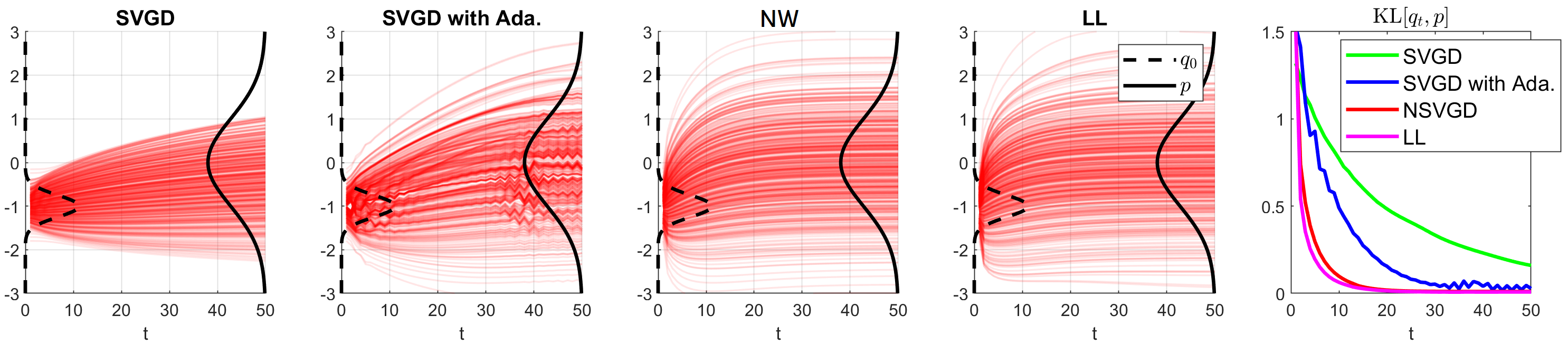
Figure 2: Particle Trajectories of SVGD, SVGD with AdaGrad, NW, LL. Approximated $\mathrm{KL}[q_{t},p]$ with different methods.

In this experiment, we investigate the performance of SVGD, NW and Local Linear (LL) estimator through the task of minimizing $\mathrm{KL}[q_{t},p]$. We let SVGD, NW and LL fit the target distribution $p=\mathcal{N}(0,1)$ by iteratively updating a particle distribution. 500 iid initial particles are drawn from $q_{0}=N(-1,0.25^{2})$. For all methods, we uses naive gradient descent to update particles with a fixed step size 0.1. However, we also consider a variant of SVGD where AdaGrad is applied to dynamically adjust the step size. For SVGD and SVGD with AdaGrad, we use the MATLAB code provided by Liu and Wang (2016) with its default settings. We plot the trajectories of particles of all three methods in Figure 2.

Although all three algorithms move particles toward the target distribution, the naive SVGD does not spread the particle mass quick enough to cover the target distribution when using the same step size. This situation is much improved by applying the adaptive learning rate. In comparison, NW and LL both converge fast. After 20 iterations, all particles have arrived at the target positions. Since all methods are motivated by minimizing $\mathrm{KL}[q_{t},p]$, we plot the $\mathrm{KL}[q_{t},p]$ approximated by Donsker and Varahan Lower Bound (Donsker and Varadhan, 1976) for all three methods. The plot of $\mathrm{KL}[q_{t},p]$ agrees with the qualitative assessments in previous plots: AdaGrad SVGD can reduce the KL significantly faster than the vanilla SVGD with naive gradient descent. After 20 iterations, the KL divergence for NW and LL particles reaches zero, indicating that the particles have fully converged to the target distribution. LL achieves a performance comparable to NW. This is a remarkable result as NW and SVGD have access to the true $\nabla\log p$ but LL only has samples from $p$.

In the next sections, we will showcase the performance of LL in forward/backward KL minimization problems.

5.2 Joint Domain Adaptation

In domain adaptation, we want to use source domain samples to help the prediction in a target domain. This addresses situations where the training data for a method may not arise from real-world scenarios when deployed. We assume that source samples $\mathcal{D}_{q}:=\left\{({\boldsymbol{x}}_{q}^{(i)},y_{q}^{(i)})\right\}_{i=1}^{n_{q}}$ are drawn from a joint distribution $\mathbb{Q}_{XY}$ and target samples $\mathcal{D}_{p}:=\left\{({\boldsymbol{x}}_{p}^{(i)},y_{p}^{(i)})\right\}_{i=1}^{n_{p}}$ are drawn from a different joint distribution $\mathbb{P}_{XY}$. However, $y_{p}$ are missing from the target set. Thus, we want to predict missing labels in $\mathcal{D}_{p}$ with the help of $\mathcal{D}_{q}$. Courty et al. (2017b, a) propose to find an optimal map that aligns the distribution $\mathbb{Q}_{XY}$ and $\mathbb{P}_{XY}$, then train a classifier on the aligned source samples. Inspired by this method, we propose to align samples by minimizing $\mathrm{KL}[q_{t},p]$, where $p$ is the density of the target $\mathbb{P}_{XY}$ and $q_{t}$ is a particle-label pair distribution whose samples are $\mathcal{D}_{q_{t}}:=\left\{({\boldsymbol{x}}_{t}^{(i)},y_{q}^{(i)})\right\}_{i=1}^{n_{q}}$. To minimize $\mathrm{KL}[q_{t},p]$, we evolve ${\boldsymbol{x}}_{t}$ according to the backward KL field and ${\boldsymbol{x}}_{t=0}$ is initialized to be the source input ${\boldsymbol{x}}_{q}$. In words, we transport source input samples so that the transported and target samples are aligned in terms of minimizing the backward KL divergence. After $T$ iterations, we can train a classifier using transported source samples $\{({\boldsymbol{x}}_{T},y)\}$ to predict target labels.

One slight issue is that we do not have labels in the target domain but performing WGF requires joint samples $(X,Y)$. To solve this, we adopt the same approach used in Courty et al. (2017a), replacing $y_{p}$ with a proxy $\hat{g}({\boldsymbol{x}}_{p})$, where $\hat{g}$ is a prediction function trained to minimize an empirical transportation cost (See Section 2.2 in Courty et al. (2017a)). We demonstrate our approach in a toy example, in Figure 3.

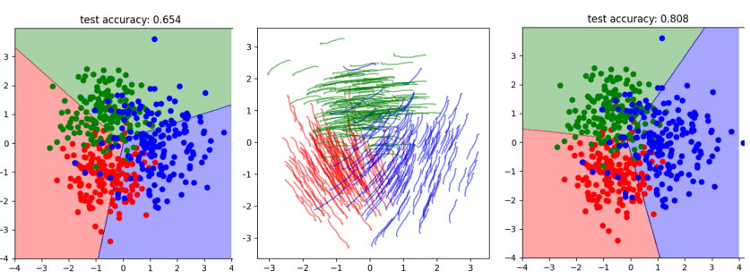
Figure 3: Left: the source classifier misclassifies many testing points. Middle: WGF moves particles to align the source samples with the target samples. Lines are trajectories of sample movements in each class. Right: the retrained classifier on the transported source samples gives a much better prediction.

Table 2 compares the performance of adapted classifiers on a real-world 10-class classification dataset named “office-caltech-10”, where images of the same objects are taken from four different domains (amazon, caltech, dslr and webcam). We reduce the dimensionality by projecting all samples to the a 100-dimensional subspace using PCA. We compare the performance of the base (the source RBF kernel SVM classifier), the Joint Distribution Optimal Transport (Courty et al., 2017a) (jdot), $\hat{g}$ in the last iteration of WGF (wgf) and an RBF kernel SVM re-trained on the transported source sample $\{({\boldsymbol{x}}_{T},y)\}$ (wgf-svm). The classification accuracy on the entire target sets are reported. It can be seen that in some cases, reusing the source classifiers in the target domain does lead to catastrophic results (e.g. amazon to dslr, caltech to dslr). However, by using any joint distribution based domain adaptation, we can avoid such performance decline. It can also be seen that the classifier $\hat{g}$ in the last WGF iteration already achieves significant improvement comparing to jdot. The SVM retrained on the transported source samples can elevate the performance even more.

$\mathcal{D}_{p}\to\mathcal{D}_{q}$	base	jdot	wgf	wgf-svm
amz.$\to$dslr	0.2739	0.6561	0.7452*	0.7834*
amz.$\to$web.	0.6169	0.678	0.7932*	0.8407*
amz.$\to$cal.	0.8166	0.6367	0.8353*	0.8272*
dslr$\to$amz.	0.7035	0.7349	0.8257*	0.8591*
dslr$\to$web.	0.9492*	0.7661	0.8746	0.9525*
dslr$\to$cal.	0.5895	0.7231	0.8139*	0.7925*
web.$\to$amz.	0.7578	0.7537	0.8831*	0.9134*
web.$\to$dslr	0.9427*	0.7325	0.8471	0.9873*
web.$\to$cal.	0.6705	0.6349	0.8103*	0.7809*
cal.$\to$amz.	0.834	0.8455	0.8935*	0.9113*
cal.$\to$dslr	0.2611	0.6943	0.7834*	0.8471*
cal.$\to$web.	0.6339	0.7458	0.7797*	0.8034*

Table 2: Domain adaptation of different domains in Office-Caltech-10 dataset. The best and second best is marked by $*$.

5.3 Missing Data Imputation

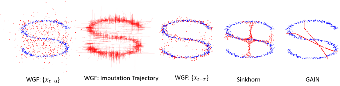
Figure 4: Comparison of imputation methods. Fully observed samples are plotted in blue and imputed samples are plotted in red. The leftmost plot shows the initial particles in WGF impute. The second left plot visualizes the imputation trajectories of different particles. The third left plot is the final output after 100 WGF iterations.

In missing data imputation, we are given a joint dataset $\tilde{\mathcal{D}}:=\{(\tilde{{\boldsymbol{x}}}^{(i)},{\boldsymbol{m}}^{(i)})\}$, where ${\boldsymbol{m}}\in\{0,1\}^{d}$ is a mask vector and $m_{j}^{(i)}=0$ indicates the $j$-th dimension of $\tilde{{\boldsymbol{x}}}^{(i)}$ is missing. The task is to “guess” the missing values in $\tilde{{\boldsymbol{x}}}$ vector. In recent years, GAN-based missing value imputation (Yoon et al., 2018) has gained significant attention. Let ${\boldsymbol{x}}$ be an imputation of $\tilde{{\boldsymbol{x}}}$. The basic idea is that if ${\boldsymbol{x}}$ is a perfect imputation of $\tilde{{\boldsymbol{x}}}$, then a classifier cannot predict $m_{j}$ given $({\boldsymbol{x}},{\boldsymbol{m}}_{-j})$. For example, given a perfectly imputed image, one cannot tell which pixels are imputed, which pixels are observed. Therefore, in their approach, a generative network is trained to minimize the aforementioned classification accuracy. In fact, this method teaches the generator to break the dependency between ${\boldsymbol{x}}$ and ${\boldsymbol{m}}$. Inspired by this idea, we propose to impute $\{\tilde{{\boldsymbol{x}}}\}$ by iteratively updating particles $\{{\boldsymbol{x}}_{t}\}$. The initial particle ${\boldsymbol{x}}_{t=0}$ is set to be

$$x_{0,j}=\begin{cases}\tilde{x}_{j}&m_{j}=1\\ \text{Sample from }\mathcal{N}(0,1)&m_{j}=0.\end{cases}$$

After that, the particles $\{{\boldsymbol{x}}_{t}\}$ are evolved according to the forward KL field that minimizes $\mathrm{KL}[p_{X_{t}M},p_{X_{t}}p_{M}]$, i.e., the mutual information between $X_{t}$ (particles) and $M$ (mask). Note that we only update missing dimensions, i.e.,

$$x_{t+1,j}:=\begin{cases}x_{t,j}&m_{j}=1\\ x_{t,j}+\eta\partial_{x_{j}}r_{t}({\boldsymbol{x}}_{t},{\boldsymbol{m}})&m_{j}=0.\end{cases}$$

Samples from $p_{X_{t}M}$ are available to us since we observe the pairs $\{({\boldsymbol{x}},{\boldsymbol{m}})\}$ and samples from $p_{X_{t}}p_{M}$ can be constructed as $\{({\boldsymbol{x}},{\boldsymbol{m}}^{\prime})\}$, where ${\boldsymbol{m}}^{\prime}$ is a random sample of $M$ given the missing pattern.

In the first experiment, we test the performance of various imputers on an “S”-shaped dataset, where samples are Missing Completely at Random (MCAR) (Donders et al., 2006). The results are plotted in Figure 4. We compare our imputed results (WGF) with Optimal Transport-based imputation (Muzellec et al., 2020) (sinkhorn) and GAN-based imputation (GAIN). $\sigma$ is chosen by automatic model selection described in Section I.1. It can be seen that our imputer, based on minimizing $\mathrm{KL}[p_{X_{t}M}|p_{X_{t}}p_{M}]$ nicely recovers the “S”-shape after 100 particle update iterations. However, Sinkhorn and GAIN imputation does not recover the “S”-shape well.

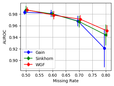
Figure 5: AUROC of a linear SVM classifier on the imputed Breast Cancer dataset

Finally, we test the performance of our algorithm on a real-world Breast Cancer classification dataset (Zwitter and Soklic, 1988) in Figure 5. This is a 30-dimensional binary classification dataset and we artificially create missing values by following MCAR paradigm with different missing rates. Since the dataset is a binary classification dataset, we compare the performance of linear SVM classifiers trained on imputed datasets. The performance is measured by Area Under the ROC curve (AUROC) on hold out testing sets. The result shows, SVM trained on the dataset imputed by our method, achieves comparable performance to datasets imputed by two other state-of-the-art methods, GAIN and sinkhorn. Details of the hyperparameter setting can be found in Section I.2

6 Impact Statement

This paper presents work whose goal is to advance the field of Machine Learning. There are many potential societal consequences of our work, none which we feel must be specifically highlighted here.

Appendix A Proof of Proposition 3.1

Proof.

$$\left|\hat{u}_{i}({\boldsymbol{x}}^{\star})-\partial_{i}\log r({\boldsymbol{x}}^{\star})\right|= \left|\frac{\widehat{\mathbb{E}}_{q}\left[k_{\sigma}({\boldsymbol{x}},{\boldsymbol{x}}^{\star})\partial_{i}\log r({\boldsymbol{x}})\right]}{\widehat{\mathbb{E}}_{q}[k_{\sigma}({\boldsymbol{x}},{\boldsymbol{x}}^{\star})]}-\partial_{i}\log r({\boldsymbol{x}}^{\star})\right|$$

$$= \left|\frac{\widehat{\mathbb{E}}_{q}[k_{\sigma}({\boldsymbol{x}},{\boldsymbol{x}}^{\star})\left(\partial_{i}\log r({\boldsymbol{x}}^{\star})+\langle\nabla\partial_{i}\log r(\bar{{\boldsymbol{x}}}),{\boldsymbol{x}}-{\boldsymbol{x}}^{\star}\rangle\right)]}{\widehat{\mathbb{E}}_{q}[k_{\sigma}({\boldsymbol{x}},{\boldsymbol{x}}^{\star})]}-\partial_{i}\log r({\boldsymbol{x}}^{\star})\right|$$

$$= \left|\frac{\widehat{\mathbb{E}}_{q}[k_{\sigma}({\boldsymbol{x}},{\boldsymbol{x}}^{\star})\langle\nabla\partial_{i}\log r(\bar{{\boldsymbol{x}}}),{\boldsymbol{x}}-{\boldsymbol{x}}^{\star}\rangle]}{\widehat{\mathbb{E}}_{q}[k_{\sigma}({\boldsymbol{x}},{\boldsymbol{x}}^{\star})]}\right|$$

$$\leq \frac{\widehat{\mathbb{E}}_{q}[k_{\sigma}({\boldsymbol{x}},{\boldsymbol{x}}^{\star})\|\nabla\partial_{i}\log r(\bar{{\boldsymbol{x}}})\|\cdot\|{\boldsymbol{x}}-{\boldsymbol{x}}^{\star}\|]}{\widehat{\mathbb{E}}_{q}[k_{\sigma}({\boldsymbol{x}},{\boldsymbol{x}}^{\star})]}$$

$$\leq \kappa\cdot\frac{\widehat{\mathbb{E}}_{q}[k_{\sigma}({\boldsymbol{x}},{\boldsymbol{x}}^{\star})\|{\boldsymbol{x}}-{\boldsymbol{x}}^{\star}\|]}{\widehat{\mathbb{E}}_{q}[k_{\sigma}({\boldsymbol{x}},{\boldsymbol{x}}^{\star})]}$$

$$\leq \kappa\cdot\left(\frac{\widehat{\mathbb{E}}_{q}[k_{\sigma}({\boldsymbol{x}},{\boldsymbol{x}}^{\star})\|{\boldsymbol{x}}-{\boldsymbol{x}}^{\star}\|]}{\widehat{\mathbb{E}}_{q}[k_{\sigma}({\boldsymbol{x}},{\boldsymbol{x}}^{\star})]}-\frac{\mathbb{E}_{q}[k_{\sigma}({\boldsymbol{x}},{\boldsymbol{x}}^{\star})\|{\boldsymbol{x}}-{\boldsymbol{x}}^{\star}\|]}{\mathbb{E}_{q}[k_{\sigma}({\boldsymbol{x}},{\boldsymbol{x}}^{\star})]}+\frac{\mathbb{E}_{q}[k_{\sigma}({\boldsymbol{x}},{\boldsymbol{x}}^{\star})\|{\boldsymbol{x}}-{\boldsymbol{x}}^{\star}\|]}{\mathbb{E}_{q}[k_{\sigma}({\boldsymbol{x}},{\boldsymbol{x}}^{\star})]}\right)$$ (17)

The second line is due to the mean value theorem and $\bar{{\boldsymbol{x}}}$ is a point in between ${\boldsymbol{x}}$ and ${\boldsymbol{x}}^{\star}$ in a coordinate-wise fashion. The second inequality is due to the operator norm of a matrix is always greater than a row/column norm.

Since $\mathrm{Var}_{q}[\frac{1}{\sigma^{d}}k_{\sigma}({\boldsymbol{x}},{\boldsymbol{x}}^{\star})\|{\boldsymbol{x}}-{\boldsymbol{x}}^{\star}\|]=O(\frac{1}{{\sigma^{d}}})$ due to the assumption, using Chebyshev inequality

$$\widehat{\mathbb{E}}_{q}\left[\frac{1}{\sqrt{n\sigma^{d}}}k_{\sigma}({\boldsymbol{x}},{\boldsymbol{x}}^{\star})\|{\boldsymbol{x}}-{\boldsymbol{x}}^{\star}\|\right]-\mathbb{E}_{q}\left[\frac{1}{\sqrt{n\sigma^{d}}}k_{\sigma}({\boldsymbol{x}},{\boldsymbol{x}}^{\star})\|{\boldsymbol{x}}-{\boldsymbol{x}}^{\star}\|\right]=O_{p}(\frac{1}{\sqrt{n\sigma^{d}}}).$$

Similarly, due to the assumption that $\mathrm{Var}_{q}[\frac{1}{\sigma^{d}}k_{\sigma}({\boldsymbol{x}},{\boldsymbol{x}}^{\star})]=O(\frac{1}{{\sigma^{d}}})$, we have

$$\widehat{\mathbb{E}}_{q}\left[\frac{1}{\sqrt{n\sigma^{d}}}k_{\sigma}({\boldsymbol{x}},{\boldsymbol{x}}^{\star})\right]-\mathbb{E}_{q}\left[\frac{1}{\sqrt{n\sigma^{d}}}k_{\sigma}({\boldsymbol{x}},{\boldsymbol{x}}^{\star})\right]=O_{p}(\frac{1}{\sqrt{n\sigma^{d}}}).$$

Lemma A.1.

Suppose $|\mathbb{E}A|\leq A_{1}<\infty,|\mathbb{E}B|>B_{0}>0$. $\widehat{\mathbb{E}}A-\mathbb{E}{A}=O_{p}(\frac{1}{\sqrt{n\sigma^{d}}})$ and $\widehat{\mathbb{E}}B-\mathbb{E}{B}=O_{p}(\frac{1}{\sqrt{n\sigma^{d}}})$

$$\frac{\widehat{\mathbb{E}}A}{\widehat{\mathbb{E}}B}-\frac{\mathbb{E}{A}}{{\mathbb{E}{B}}}=O_{p}\left(\frac{1}{\sqrt{n\sigma^{d}}}\right).$$

Proof.

$\left|\frac{\widehat{\mathbb{E}}A}{\widehat{\mathbb{E}}B}-\frac{\mathbb{E}{A}}{{\mathbb{E}{B}}}\right|=\left|\frac{\widehat{\mathbb{E}}A\mathbb{E}B-\mathbb{E}A\widehat{\mathbb{E}}B}{\widehat{\mathbb{E}}B\mathbb{E}{B}}\right|\leq\left|\frac{\widehat{\mathbb{E}}A-\mathbb{E}A}{\mathbb{E}{B}}\right|+\left|\frac{\widehat{\mathbb{E}}B-\mathbb{E}B}{\widehat{\mathbb{E}}B\mathbb{E}{B}}\right|\cdot|\mathbb{E}A|$. First, due to the boundedness of $\mathbb{E}B$, $\left|\frac{\widehat{\mathbb{E}}A-\mathbb{E}A}{\mathbb{E}{B}}\right|=O_{p}(\frac{1}{\sqrt{n\sigma^{d}}})$. Second, due to the boundedness of $|\mathbb{E}A|,|\mathbb{E}B|$ and the fact that $\exists N,\forall n>N$, $|\widehat{\mathbb{E}}B|>|\mathbb{E}B/2|$ with a probability $1-\epsilon$, for any $\epsilon$, $\left|\frac{\widehat{\mathbb{E}}B-\mathbb{E}B}{\widehat{\mathbb{E}}B\mathbb{E}{B}}\right|\cdot|\mathbb{E}A|=O_{p}(\frac{1}{\sqrt{n\sigma^{d}}})$. Hence, $\frac{\widehat{\mathbb{E}}A}{\widehat{\mathbb{E}}B}-\frac{\mathbb{E}{A}}{{\mathbb{E}{B}}}=O_{p}\left(\frac{1}{\sqrt{n\sigma^{d}}}\right).$ ∎

Due to Lemma A.1 and (17), we have

$$\left|\hat{u}_{i}({\boldsymbol{x}}^{\star})-\partial_{i}\log r({\boldsymbol{x}}^{\star})\right|\leq \kappa\cdot\left(O_{p}(\frac{1}{\sqrt{n\sigma^{d}}})+\frac{\mathbb{E}_{q}[k_{\sigma}({\boldsymbol{x}},{\boldsymbol{x}}^{\star})\|{\boldsymbol{x}}-{\boldsymbol{x}}^{\star}\|]}{\mathbb{E}_{q}[k_{\sigma}({\boldsymbol{x}},{\boldsymbol{x}}^{\star})]}\right)$$

$$\leq \kappa\cdot\left(O_{p}(\frac{1}{\sqrt{n\sigma^{d}}})+\frac{\sigma\int q({\boldsymbol{x}}^{\star}+\sigma{\boldsymbol{y}})k({\boldsymbol{y}})\|{\boldsymbol{y}}\|\mathrm{d}{\boldsymbol{y}}}{\int q({\boldsymbol{x}}^{\star}+\sigma{\boldsymbol{y}})k({\boldsymbol{y}})\mathrm{d}{\boldsymbol{y}}}\right)~{}~{}~{}~{}~{}~{}~{}~{}~{}~{}~{}~{}~{}{\boldsymbol{y}}:=({\boldsymbol{x}}-{\boldsymbol{x}}^{\star})/\sigma$$

$$\leq \kappa\cdot\left(O_{p}(\frac{1}{\sqrt{n\sigma^{d}}})+\sigma C_{k}\right)$$

∎

Appendix B Visualization of Gradient Estimation using Local Linear Fitting

Figure 6: Fit $g$ locally at ${\boldsymbol{x}}^{\star}$ using a linear function $\hat{g}$. Its “slope” is a natural estimator of $\nabla_{\boldsymbol{x}}g({\boldsymbol{x}}^{\star})$.

Appendix C Variational Objective for Estimating $h\circ r$

Proposition C.1.

The supremum in (9) is attained if and only if $d=h\circ r$.

Proof.

Due to the maximizing argument, the supremum of (9) is attained if and only if $d=\psi^{\prime}$. The definition of mirror divergence states that $\psi^{\prime}=r\phi^{\prime}(r)-\phi(r)=h(r).$ The last equality is due to the definition of $h$ in Theorem 2.1, thus the supremum is attained if and only if $d=h\circ r$. ∎

Appendix D Proof of Theorem 4.8, Asymptotic Consistency of ${\boldsymbol{w}}({\boldsymbol{x}}^{\star})$

Proof.

In this section, to simplify notations, we denote ${\boldsymbol{\theta}}$ as the parameter vector that combines both ${\boldsymbol{w}}$ and $b$, i.e., ${\boldsymbol{\theta}}:=[{\boldsymbol{w}},b]^{\top}$. Specifically, we define

$${\boldsymbol{\theta}}^{*}=\left[{{\boldsymbol{w}}^{*}}^{\top},b^{*}\right]^{\top}:=\left[\nabla^{\top}(h\circ r)({\boldsymbol{x}}^{\star}),h(r({\boldsymbol{x}}^{\star}))-\langle\nabla(h\circ r)({\boldsymbol{x}}^{\star}),{\boldsymbol{x}}^{\star}\rangle\right]^{\top}.$$

Let us denote the negative objective function in (4.2) as $\ell({\boldsymbol{\theta}})$ and consider a constrained optimization problem:

$$\min_{\boldsymbol{\theta}}\ell({\boldsymbol{\theta}})\text{ subject to:}\|{\boldsymbol{\theta}}-{\boldsymbol{\theta}}^{*}\|^{2}\leq\min(W,B)^{2}.$$ (18)

This convex optimization has a Lagrangian $\ell({\boldsymbol{\theta}})+\lambda(\|{\boldsymbol{\theta}}-{\boldsymbol{\theta}}^{*}\|^{2}-\min(W,B)^{2})$, where $\lambda\geq 0$ is the Lagrangian multiplier. According to KKT condition, the optimal solution ${\boldsymbol{\theta}}_{0}$ of (18) satisfies $\nabla\ell({\boldsymbol{\theta}}_{0})+2\lambda({\boldsymbol{\theta}}_{0}-{\boldsymbol{\theta}}^{*})={\boldsymbol{0}}$.

We apply mean value theorem to $g({\boldsymbol{\theta}}):=\langle{\boldsymbol{\theta}}_{0}-{\boldsymbol{\theta}}^{*},\nabla\ell({\boldsymbol{\theta}})+2\lambda({\boldsymbol{\theta}}-{\boldsymbol{\theta}}^{*})\rangle$:

$$\underbrace{\langle{\boldsymbol{\theta}}_{0}-{\boldsymbol{\theta}}^{*},\nabla\ell({\boldsymbol{\theta}}_{0})+2\lambda({\boldsymbol{\theta}}_{0}-{\boldsymbol{\theta}}^{*})}_{g({\boldsymbol{\theta}}_{0})=0,\text{ KKT condition}}\rangle=\underbrace{\langle{\boldsymbol{\theta}}_{0}-{\boldsymbol{\theta}}^{*},\nabla\ell({\boldsymbol{\theta}}^{*})\rangle}_{g({\boldsymbol{\theta}}^{*})}+\langle\underbrace{({\boldsymbol{\theta}}_{0}-{\boldsymbol{\theta}}^{*})^{\top}\left[\nabla^{2}\ell(\bar{{\boldsymbol{\theta}}})+2\lambda{\boldsymbol{I}}\right]}_{\nabla g(\bar{{\boldsymbol{\theta}}})},({\boldsymbol{\theta}}_{0}-{\boldsymbol{\theta}}^{*})\rangle,$$

where $\bar{{\boldsymbol{\theta}}}$ is a point between ${\boldsymbol{\theta}}^{*}$ and ${\boldsymbol{\theta}}_{0}$ in an elementwise fashion. Since $\bar{{\boldsymbol{\theta}}}$ is in a hyper cube with ${\boldsymbol{\theta}}_{0}$ and ${\boldsymbol{\theta}}^{*}$ as opposite corners, it is in the constrain set of (18). Let us rearrange terms:

$$-\langle{\boldsymbol{\theta}}_{0}-{\boldsymbol{\theta}}^{*},\nabla\ell({\boldsymbol{\theta}}^{*})\rangle=\langle{\boldsymbol{\theta}}_{0}-{\boldsymbol{\theta}}^{*},\left[\nabla^{2}\ell(\bar{{\boldsymbol{\theta}}})+2\lambda{\boldsymbol{I}}\right]({\boldsymbol{\theta}}_{0}-{\boldsymbol{\theta}}^{*})\rangle\geq\langle{\boldsymbol{\theta}}_{0}-{\boldsymbol{\theta}}^{*},\nabla^{2}\ell(\bar{{\boldsymbol{\theta}}})({\boldsymbol{\theta}}_{0}-{\boldsymbol{\theta}}^{*})\rangle,$$

For all ${\boldsymbol{\theta}}$ in the constraint set, $\|{\boldsymbol{w}}\|=\|{\boldsymbol{w}}-{\boldsymbol{w}}^{*}+{\boldsymbol{w}}^{*}\|\leq\|{\boldsymbol{w}}-{\boldsymbol{w}}^{*}\|+\|{\boldsymbol{w}}^{*}\|\leq\|{\boldsymbol{\theta}}-{\boldsymbol{\theta}}^{*}\|+\|{\boldsymbol{w}}^{*}\|\leq 2W$ and $|b|=|b-b^{*}+b^{*}|\leq|b-b^{*}|+|b^{*}|\leq\|{\boldsymbol{\theta}}-{\boldsymbol{\theta}}^{*}\|+|b^{*}|\leq 2B$. Under our assumption (14), the lowest eigenvalue of $\nabla^{2}\ell({\boldsymbol{\theta}})$ for all ${\boldsymbol{\theta}}$ in the constrain set of (18) is always lower bounded by $\sigma^{2}\Lambda_{\mathrm{min}}$. Therefore,

$$-\langle{\boldsymbol{\theta}}_{0}-{\boldsymbol{\theta}}^{*},\nabla\ell({\boldsymbol{\theta}}^{*})\rangle\geq\sigma^{d}\cdot\Lambda_{\mathrm{min}}\|{\boldsymbol{\theta}}_{0}-{\boldsymbol{\theta}}^{*}\|^{2}.$$

Using Cauchy–Schwarz inequality

$$\|{\boldsymbol{\theta}}_{0}-{\boldsymbol{\theta}}^{*}\|\|\nabla\ell({\boldsymbol{\theta}}^{*})\|\geq\sigma^{d}\cdot\Lambda_{\mathrm{min}}\|{\boldsymbol{\theta}}_{0}-{\boldsymbol{\theta}}^{*}\|^{2}.$$

Assume $\|{\boldsymbol{\theta}}_{0}-{\boldsymbol{\theta}}^{*}\|$ is not zero (if it is, our estimator is already unbiased).

$$\|{\boldsymbol{\theta}}_{0}-{\boldsymbol{\theta}}^{*}\|\leq \frac{1}{\sigma^{d}\Lambda_{\mathrm{min}}}\|\nabla\ell({\boldsymbol{\theta}}^{*})\|$$

$$\leq \frac{1}{\sigma^{d}\Lambda_{\mathrm{min}}}\|\nabla\ell({\boldsymbol{\theta}}^{*})-\mathbb{E}\nabla\ell({\boldsymbol{\theta}}^{*})+\mathbb{E}\nabla\ell({\boldsymbol{\theta}}^{*})\|$$

$$\leq \frac{1}{\sigma^{d}\Lambda_{\mathrm{min}}}\left(\|\nabla\ell({\boldsymbol{\theta}}^{*})-\mathbb{E}\nabla\ell({\boldsymbol{\theta}}^{*})\|+\|\mathbb{E}\nabla\ell({\boldsymbol{\theta}}^{*})\|\right)$$ (19)

Since $\mathrm{tr}\left[{\mathrm{Cov}_{q}\left[\frac{1}{\sigma^{d}}{k({\boldsymbol{x}},{\boldsymbol{x}}^{\star})\cdot\tilde{{\boldsymbol{x}}}}\right]}\right]=O(\frac{1}{{\sigma^{d}}})$ and $\mathrm{tr}\left[{\mathrm{Cov}_{q}\left[\frac{1}{\sigma^{d}}{k({\boldsymbol{x}},{\boldsymbol{x}}^{\star})\cdot\psi_{\mathrm{con}}(\langle{\boldsymbol{w}}^{*},{\boldsymbol{x}}\rangle+b^{*})\tilde{{\boldsymbol{x}}}}\right]}\right]=O(\frac{1}{{\sigma^{d}}})$ by assumption, due to Chebyshev’s inequality, $\|\nabla\ell({\boldsymbol{\theta}}^{*})-\mathbb{E}\nabla\ell({\boldsymbol{x}}^{*})\|=\sigma^{d}O_{p}(\frac{1}{n\sigma^{d}})$. Therefore,

$$\|{\boldsymbol{\theta}}_{0}-{\boldsymbol{\theta}}^{*}\|\leq\frac{1}{\sigma^{d}\Lambda_{\mathrm{min}}}\left(\sigma^{d}\cdot O_{p}(\frac{1}{\sqrt{n\sigma^{d}}})+\|\mathbb{E}\nabla\ell({\boldsymbol{\theta}}^{*})\|\right)$$

Now we proceed to bound $\|\mathbb{E}\nabla\ell({\boldsymbol{\theta}}^{*})\|$.

Lemma D.1.

$\|\mathbb{E}\nabla\ell({\boldsymbol{\theta}}^{*})\|\leq\mathbb{E}_{q}\left[k_{\sigma}({\boldsymbol{x}},{\boldsymbol{x}}^{\star})\frac{1}{2}\left\|{\boldsymbol{x}}-{\boldsymbol{x}}^{\star}\right\|^{2}\|\tilde{{\boldsymbol{x}}}\|\right]\kappa\cdot C_{\psi_{\mathrm{con}}^{\prime\prime}}$

Proof.

The expression of $\mathbb{E}\nabla\ell({\boldsymbol{\theta}}^{*})$ is:

$$\mathbb{E}\nabla\ell({\boldsymbol{\theta}}^{*}):=-\mathbb{E}_{p}\left[{k_{\sigma}({\boldsymbol{x}},{\boldsymbol{x}}^{\star})}\cdot\tilde{{\boldsymbol{x}}}\right]+\mathbb{E}_{q}\left[k_{\sigma}({\boldsymbol{x}},{\boldsymbol{x}}^{\star})\psi^{\prime}_{\mathrm{con}}(\langle{\boldsymbol{w}}^{*},{\boldsymbol{x}}\rangle+b^{*})\cdot\tilde{{\boldsymbol{x}}}\right].$$ (20)

Due to Taylor’s theorem, $\langle{\boldsymbol{w}}^{*},{\boldsymbol{x}}\rangle+b^{*}=h(r({\boldsymbol{x}}))-\frac{1}{2}\left({\boldsymbol{x}}-{\boldsymbol{x}}^{\star}\right)^{\top}\nabla^{2}(h\circ r)(\bar{{\boldsymbol{x}}})\left({\boldsymbol{x}}-{\boldsymbol{x}}^{\star}\right)$ where $\bar{{\boldsymbol{x}}}$ is a point in between ${\boldsymbol{x}}$ and ${\boldsymbol{x}}^{\star}$ in an elementwise fashion. Thus, applying the mean value theorem on $\psi^{\prime}_{\mathrm{con}}$,

$$\psi_{\mathrm{con}}^{\prime}(\langle{\boldsymbol{w}}^{*},{\boldsymbol{x}}\rangle+b^{*}) =\psi_{\mathrm{con}}^{\prime}\left[h(r({\boldsymbol{x}}))-\frac{1}{2}\left({\boldsymbol{x}}-{\boldsymbol{x}}^{\star}\right)^{\top}\nabla^{2}(h\circ r)(\bar{{\boldsymbol{x}}})\left({\boldsymbol{x}}-{\boldsymbol{x}}^{\star}\right)\right]$$

$$=\psi_{\mathrm{con}}^{\prime}\left[h(r({\boldsymbol{x}}))\right]-\frac{1}{2}\left({\boldsymbol{x}}-{\boldsymbol{x}}^{\star}\right)^{\top}\nabla^{2}(h\circ r)(\bar{{\boldsymbol{x}}})\left({\boldsymbol{x}}-{\boldsymbol{x}}^{\star}\right)\psi_{\mathrm{con}}^{\prime\prime}(y),$$

where $y$ is a scalar in between $h(r({\boldsymbol{x}}))$ and $h(r({\boldsymbol{x}}))-\frac{1}{2}\left({\boldsymbol{x}}-{\boldsymbol{x}}^{\star}\right)^{\top}\nabla^{2}(h\circ r)(\bar{{\boldsymbol{x}}})\left({\boldsymbol{x}}-{\boldsymbol{x}}^{\star}\right)$ or equivalently, in between $h(r({\boldsymbol{x}}))$ and $\langle{\boldsymbol{w}}^{*},{\boldsymbol{x}}\rangle+b^{*}$.

Theorem 2.1 states that $h(r)=r\phi^{\prime}+\phi$, then, by the definition of the mirror divergence, $\psi^{\prime}=h(r)$. Moreover, due to the maximizing argument, $\psi^{\prime}_{\mathrm{con}}$ is the input argument of $\psi$ (i.e., $r$) and $\psi^{\prime}$ is the input argument of $\psi_{\mathrm{con}}$. Thus, $\psi_{\mathrm{con}}^{\prime}(h(r))=\psi^{\prime}_{\mathrm{con}}(\psi^{\prime}(r))=r$. Let us write

$$\mathbb{E}\nabla\ell({\boldsymbol{\theta}}^{*}) =-\mathbb{E}_{p}[k_{\sigma}({\boldsymbol{x}},{\boldsymbol{x}}^{\star})\tilde{{\boldsymbol{x}}}]+\mathbb{E}_{q}[k_{\sigma}({\boldsymbol{x}},{\boldsymbol{x}}^{\star})\underbrace{\psi_{\mathrm{con}}^{\prime}(h(r({\boldsymbol{x}})))}_{r}\tilde{{\boldsymbol{x}}}]$$

$$~{}~{}-\mathbb{E}_{q}\left[k_{\sigma}({\boldsymbol{x}},{\boldsymbol{x}}^{\star})\frac{1}{2}\left({\boldsymbol{x}}-{\boldsymbol{x}}^{\star}\right)^{\top}\nabla^{2}(h\circ r)(\bar{{\boldsymbol{x}}})\left({\boldsymbol{x}}-{\boldsymbol{x}}^{\star}\right)\psi_{\mathrm{con}}^{\prime\prime}(y)\tilde{{\boldsymbol{x}}}\right]$$

$$=-\mathbb{E}_{q}\left[k_{\sigma}({\boldsymbol{x}},{\boldsymbol{x}}^{\star})\frac{1}{2}\left({\boldsymbol{x}}-{\boldsymbol{x}}^{\star}\right)^{\top}\nabla^{2}(h\circ r)(\bar{{\boldsymbol{x}}})\left({\boldsymbol{x}}-{\boldsymbol{x}}^{\star}\right)\psi_{\mathrm{con}}^{\prime\prime}(y)\tilde{{\boldsymbol{x}}}\right],$$

We can derive a bound for $\|\mathbb{E}\nabla\ell({\boldsymbol{\theta}}^{*})\|$:

$$\|\mathbb{E}\nabla\ell({\boldsymbol{\theta}}^{*})\| \leq\mathbb{E}_{q}\left[k_{\sigma}({\boldsymbol{x}},{\boldsymbol{x}}^{\star})\cdot\frac{1}{2}\left|\left({\boldsymbol{x}}-{\boldsymbol{x}}^{\star}\right)^{\top}\nabla^{2}(h\circ r)(\bar{{\boldsymbol{x}}})\left({\boldsymbol{x}}-{\boldsymbol{x}}^{\star}\right)\right|\cdot|\psi_{\mathrm{con}}^{\prime\prime}(y)|\cdot\|\tilde{{\boldsymbol{x}}}\|\right]$$

$$\leq\mathbb{E}_{q}\left[k_{\sigma}({\boldsymbol{x}},{\boldsymbol{x}}^{\star})\frac{1}{2}\left\|{\boldsymbol{x}}-{\boldsymbol{x}}^{\star}\right\|^{2}\left\|\nabla^{2}(h\circ r)(\bar{{\boldsymbol{x}}})\right\|\|\tilde{{\boldsymbol{x}}}\|\right]C_{\psi_{\mathrm{con}}^{\prime\prime}}$$

$$\leq\mathbb{E}_{q}\left[k_{\sigma}({\boldsymbol{x}},{\boldsymbol{x}}^{\star})\frac{1}{2}\left\|{\boldsymbol{x}}-{\boldsymbol{x}}^{\star}\right\|^{2}\|\tilde{{\boldsymbol{x}}}\|\right]\kappa\cdot C_{\psi_{\mathrm{con}}^{\prime\prime}}$$

$$\leq\sigma^{d+2}\cdot\kappa\cdot C_{\psi_{\mathrm{con}}^{\prime\prime}}\int q(\sigma{\boldsymbol{y}}+{\boldsymbol{x}}^{\star})\cdot k({\boldsymbol{y}})\cdot\left\|{\boldsymbol{y}}\right\|^{2}\cdot\left\|[\sigma{\boldsymbol{y}}+{{\boldsymbol{x}}^{\star}},1]\right\|\mathrm{d}{\boldsymbol{y}}\leq\sigma^{d+2}\cdot\kappa\cdot C_{\psi_{\mathrm{con}}^{\prime\prime}}C$$

∎

Finally, due to Lemma D.1 and Assumption 4.5, we can see that

$$\|{\boldsymbol{\theta}}^{*}-{\boldsymbol{\theta}}_{0}\|\leq\frac{\sigma^{d}O_{p}(\frac{1}{n\sigma^{d}})+\kappa\cdot\sigma^{d+2}\cdot C_{k}\cdot C_{\psi_{\mathrm{con}}^{\prime\prime}}}{\sigma^{d}\Lambda_{\mathrm{min}}}\leq\frac{O_{p}(\frac{1}{n\sigma^{d}})+\kappa\cdot\sigma^{d}\cdot C_{k}\cdot C_{\psi_{\mathrm{con}}^{\prime\prime}}}{\Lambda_{\mathrm{min}}}.$$

Since $n\sigma\to\infty,\sigma\to 0$, $\|{\boldsymbol{\theta}}^{*}-{\boldsymbol{\theta}}_{0}\|\to 0$ with high probability. There always exists a $\sigma_{0}$, such that for all $\sigma<\sigma_{0}$, $\min(W,B)>\frac{\kappa\cdot C_{k}\cdot C_{\psi_{\mathrm{con}}^{\prime\prime}}\cdot\sigma^{2}}{\Lambda_{\mathrm{min}}}$. When it happens, ${\boldsymbol{\theta}}_{0}$ must be the interior of the constrain set of (18). i.e., the constraints in (18) are not active. It implies ${\boldsymbol{\theta}}_{0}$ must be the stationary point of $\ell({\boldsymbol{\theta}})$ as long as $\sigma$ is sufficiently small and $n$ is sufficiently large.

∎

Appendix E Proof of Corollary 4.9

Proof.

Since (4.2) has a unconstrained quadratic objective, its maximizers are stationary points.

We can see that Assumption 4.4 holds. To apply Theorem 4.8, we still need to show that Assumption 4.7 holds and $W$ and $B$ exist. In this case, $\psi_{\mathrm{con}}(d)=d^{2}/2+d$, so $\psi_{\mathrm{con}}^{\prime\prime}=1$. Thus Assumption 4.7 holds automatically for every $C_{\psi_{\mathrm{con}}^{\prime\prime}}\geq 1$. Additionally,

$$\nabla_{[{\boldsymbol{w}},b]}^{2}\psi_{\mathrm{con}}(\langle{\boldsymbol{w}},{\boldsymbol{x}}\rangle+b)=\mathbb{E}_{q}[k_{\sigma}({\boldsymbol{x}},{\boldsymbol{x}}^{\star})\psi^{\prime\prime}(\langle{\boldsymbol{w}},{\boldsymbol{x}}\rangle+b)\tilde{{\boldsymbol{x}}}\tilde{{\boldsymbol{x}}}^{\top}]=\mathbb{E}_{q}[k_{\sigma}({\boldsymbol{x}},{\boldsymbol{x}}^{\star})\tilde{{\boldsymbol{x}}}\tilde{{\boldsymbol{x}}}^{\top}].$$

(15) implies the minimum eigenvalue assumption (14) holds for every $W>0,B>0$. Thus, we can choose any $W>0$ and $B>0$ that satisfies (13). Noticing that $h(r({\boldsymbol{x}}))=r({\boldsymbol{x}})$, applying Theorem 4.8 gives the desired result. ∎

Appendix F Proof of Corollary 4.10

Proof.

Assumption 4.4, 4.5 and (13) are already satisfied. Let us verify the eigenvalue condition (14). In this case, $\psi_{\mathrm{con}}^{\prime\prime}(d)=\exp(d-1)$. Thus $\exp(\langle{\boldsymbol{w}},{\boldsymbol{x}}\rangle+b-1)\leq\exp(2WC_{\mathcal{X}}+2B-1)<\infty$ for $\|{\boldsymbol{w}}\|\leq 2W,|b|\leq 2B$. Moreover, because $\tilde{{\boldsymbol{x}}}\tilde{{\boldsymbol{x}}}^{\top}$ is positive semi-definite,

$$\lambda_{\mathrm{min}}\left[\mathbb{E}_{q}[k_{\sigma}({\boldsymbol{x}},{\boldsymbol{x}}^{\star})\exp(\langle{\boldsymbol{w}},{\boldsymbol{x}}\rangle+b-1)\tilde{{\boldsymbol{x}}}\tilde{{\boldsymbol{x}}}^{\top}]\right]\geq \sigma^{2}\cdot\lambda_{\mathrm{min}}\left[\mathbb{E}_{q}[k_{\sigma}({\boldsymbol{x}},{\boldsymbol{x}}^{\star})\tilde{{\boldsymbol{x}}}\tilde{{\boldsymbol{x}}}^{\top}]\right]\cdot\exp(-2WC_{\mathcal{X}}-2B-1)$$

$$> \sigma^{2}\cdot\Lambda_{\leftarrow}\cdot\exp(-2WC_{\mathcal{X}}-2B-1)>0,$$

for all ${\boldsymbol{w}},b$ that $\|{\boldsymbol{w}}\|\leq 2W,|b|\leq 2B$ due to (16). So (14) holds. Finally, let us verify Assumption 4.7. Since $\psi_{\mathrm{con}^{\prime\prime}}$ is a strictly monotone increasing function, $\sup_{a\in[0,1]}\psi_{\mathrm{con}^{\prime\prime}}(ax_{0}+(1-a)y_{0})$ is obtained either at $x_{0}$ or $y_{0}$. We only need to verify that $\psi_{\mathrm{con}^{\prime\prime}}(h(r({\boldsymbol{x}})))$ and $\psi_{\mathrm{con}^{\prime\prime}}(\langle{\boldsymbol{w}}^{*},{\boldsymbol{x}}\rangle+b^{*})$ are both bounded for all ${\boldsymbol{x}}$. Both $h(r({\boldsymbol{x}}))$ and $\langle{\boldsymbol{w}}^{*},{\boldsymbol{x}}\rangle+b^{*}$ can be bounded using our assumptions. Thus, for a

$$C_{\psi_{\mathrm{con}}^{\prime\prime}}=\exp(W\cdot C_{\mathcal{X}}+B-1)\vee\exp(C_{\log r}-1)$$

Assumption 4.7 holds. Applying Theorem 4.8 completes the proof. ∎

Appendix G $\|\nabla^{2}r({\boldsymbol{x}})\|$ for Different $p$ and $q$

(a) $p,q$ with different means. The further $p,q$ are apart, the larger the $\sup_{{\boldsymbol{x}}}\|\nabla^{2}r({\boldsymbol{x}})\|$ is.

(b) $p,q$ with different variances. The less overlapped $p,q$ are, the larger the $\sup_{{\boldsymbol{x}}}\|\nabla^{2}r({\boldsymbol{x}})\|$ is.

Figure 7: Visualizing $\nabla^{2}(h\circ r)({\boldsymbol{x}})$ for $\mathrm{D}_{\phi}=\mathrm{KL}[p,q]$ with two different settings of $p$ and $q$.

See Figure 7.

Appendix H Finite-sample Objectives

H.1 Practical Implementation

In our experiments, we observe that (4.2) can be efficiently minimized by using gradient descent with adaptive learning rate schemes, e.g., Adam (Kingma and Ba, 2015). One computational advantage of local linear model is that the computation for each ${\boldsymbol{x}}^{\star}$ is independent from the others. This property allows us to parallelize the optimization. Even using a single CPU/GPU, we can easily write highly vectorized code to compute the gradient of (4.2) with respect to ${\boldsymbol{w}}$ and $b$ for a large particle set $\textperiodcentered\{{\boldsymbol{x}}_{i}^{\star}\}_{i=1}^{n}$.

Suppose ${\boldsymbol{X}}_{p}\in\mathbb{R}^{n_{p}\times d}$ and ${\boldsymbol{X}}_{q}\in\mathbb{R}^{n_{q}\times d}$ are the matrices whose rows are ${\boldsymbol{x}}_{p}^{(i)}$ and ${\boldsymbol{x}}_{q}^{(i)}$ respectively. ${\boldsymbol{K}}_{p}\in\mathbb{R}^{n\times n_{p}}$, ${\boldsymbol{K}}_{q}\in\mathbb{R}^{n\times n_{q}}$ are the kernel matrices between $\{{\boldsymbol{x}}^{\star}\}$ and ${\boldsymbol{X}}_{p}$, $\{{\boldsymbol{x}}^{\star}\}$ and ${\boldsymbol{X}}_{q}$ respectively. ${\boldsymbol{W}}\in\mathbb{R}^{n\times d}$ and ${\boldsymbol{b}}\in\mathbb{R}^{n}$ are the parameters whose rows are ${\boldsymbol{w}}({\boldsymbol{x}}^{\star})$ and $b({\boldsymbol{x}}^{\star})$ respectively. Then the gradient of (4.2) with respect to ${\boldsymbol{W}}$, ${\boldsymbol{b}}$ can be expressed as

$${\boldsymbol{K}}_{p}{\boldsymbol{X}}_{p}/n_{p}-{\boldsymbol{K}}_{q}\odot\psi_{\text{con}}^{\prime}({\boldsymbol{W}}{\boldsymbol{X}}_{q}^{\top}+{\boldsymbol{b}}){\boldsymbol{X}}_{q}/n_{q},$$

$${\boldsymbol{K}}_{p}{\boldsymbol{1}}_{n_{p}}/n_{p}-{\boldsymbol{K}}_{q}\odot\psi_{\text{con}}^{\prime}({\boldsymbol{W}}{\boldsymbol{X}}_{q}^{\top}+{\boldsymbol{b}}){\boldsymbol{1}}_{n_{q}}/n_{q},$$

where ${\boldsymbol{1}}_{n_{p}}$ and ${\boldsymbol{1}}_{n_{q}}$ are the vectors of ones with length $n_{p}$ and $n_{q}$ respectively. $\psi_{\mathrm{con}}^{\prime}$ is evaluated element-wise. $\odot$ is the element-wise product and the vector ${\boldsymbol{b}}$ is broadcast to a matrix with $n_{q}$ columns.

Appendix I Experiment Details in Section 5

I.1 Model Selection

Let $\mathcal{D}_{p}:=\left\{{\boldsymbol{x}}_{p}^{(i)}\right\}_{i=1}^{n_{p}},\mathcal{D}_{q}:=\left\{{\boldsymbol{x}}_{q}^{(i)}\right\}_{i=1}^{n_{q}}$ be training sets from $p$ and $q$ respectively and $\tilde{\mathcal{D}}_{p}=\left\{\tilde{{\boldsymbol{x}}}_{p}^{(i)}\right\}_{i=1}^{\tilde{n}_{p}}$ and $\tilde{\mathcal{D}}_{q}=\left\{\tilde{{\boldsymbol{x}}}_{q}^{(i)}\right\}_{i=1}^{\tilde{n}_{q}}$ be testing sets. We can fit a local linear model at each testing point using the training sets, i.e.,

$$\left(\hat{{\boldsymbol{w}}}_{\sigma}(\tilde{{\boldsymbol{x}}}),\hat{b}_{\sigma}(\tilde{{\boldsymbol{x}}})\right) :=\mathop{\rm argmax}\limits_{{\boldsymbol{w}}\in\mathbb{R}^{d},b\in\mathbb{R}}\underbrace{\ell\left({\boldsymbol{w}},b;\tilde{{\boldsymbol{x}}},\mathcal{D}_{p},\mathcal{D}_{q}\right)}_{\text{tranining objective}}.$$

The dependency on $\sigma$ comes from the smoothing kernel in the training objective. We can tune $\sigma$ by evaluating the variational lower bound (9) approximated using testing samples:

$$\tilde{\ell}\left(\sigma;\tilde{\mathcal{D}}_{p},\tilde{\mathcal{D}}_{q}\right) :=\underbrace{\tilde{\mathbb{E}}_{p}\left[\hat{d}_{\sigma}\left({\boldsymbol{x}}\right)\right]-\tilde{\mathbb{E}}_{q}\left[\psi_{\text{con}}(\hat{d}_{\sigma}\left({\boldsymbol{x}}\right))\right]}_{\text{testing criterion}},$$ (21)

where $\tilde{\mathbb{E}}_{p}[\hat{d}({\boldsymbol{x}})]:=\frac{1}{\tilde{n}_{p}}\sum_{i=1}^{\tilde{n}_{p}}\hat{d}(\tilde{{\boldsymbol{x}}}_{p}^{(i)}),$ i.e., the sample average over the testing points. $\hat{d}_{\sigma}(\tilde{{\boldsymbol{x}}}):=\langle\hat{{\boldsymbol{w}}}_{\sigma}\left(\tilde{{\boldsymbol{x}}}\right),\tilde{{\boldsymbol{x}}}\rangle+\hat{b}_{\sigma}\left(\tilde{{\boldsymbol{x}}}\right)$, is the interpolation of $d(\tilde{{\boldsymbol{x}}})$ using training samples. The best choice of $\sigma$ should maximize the above testing criterion.

In our experiments, we construct training and testing sets using cross validation and choose a list of candidate $\sigma$ for the model selection. This procedure is parallel to selecting $k$ in $k$-nearest neighbors to minimize the testing error. In our case, (21) is the “negative testing error”.

I.2 Missing Data Imputation

Before running the experiments, we first pre-process data in the following way:

1. Suppose ${\boldsymbol{X}}_{\text{true}}$ is the original data matrix, i.e. without missing values. We introduce missingness to ${\boldsymbol{X}}_{\text{true}}$, and called the matrix with missing values $\tilde{{\boldsymbol{X}}}$, following MCAR paradigm. Denote the corresponding mask matrix as ${\boldsymbol{M}}$, where $m_{i,j}=0$ if ${\tilde{x}}_{i,j}$ is missing, and $m_{i,j}=1$ otherwise.

2. Calculate column-wise mean $\bar{\tilde{{\boldsymbol{x}}}}$ and standard deviation $\tilde{{\boldsymbol{s}}}$ (excluding missing values) of $\tilde{{\boldsymbol{X}}}$.

3. Standardize $\tilde{{\boldsymbol{X}}}$ by taking $\tilde{{\boldsymbol{X}}}=\frac{\tilde{{\boldsymbol{X}}}-\bar{\tilde{{\boldsymbol{x}}}}}{\tilde{{\boldsymbol{s}}}}$, where the vectors $\bar{\tilde{{\boldsymbol{x}}}}$ and $\tilde{{\boldsymbol{s}}}$ are broadcasted to the same dimensions as the matrix $\tilde{{\boldsymbol{X}}}$. Note that the division here is element-wise.

Denote ${\boldsymbol{X}}^{i}$ as the imputed data of $\tilde{{\boldsymbol{X}}}$ at iteration $i$, where ${\boldsymbol{X}}^{0}=\tilde{{\boldsymbol{X}}}\odot{\boldsymbol{M}}+\mathbf{Z}\odot(1-{\boldsymbol{M}})$, and $\mathbf{Z}\sim\mathcal{N}(\mathbf{0},\text{diag}(\mathbf{1}))$.

We performed two experiments on both toy data (”S”-shape) and real world data (UCI Breast Cancer data).

Let $N_{\text{WGF}}$ be the number of iterations WGF is performed. In each iteration, let $N_{\text{GradEst}}$ be the number gradient descent steps for gradient estimation. In the missing data experiments, we set the hyper-parameters to be:

• ”S”-shape data:$N_{\text{WGF}}=100$, $N_{\text{GradEst}}=2000$, $\sigma$ is chosen by model selection described in Section I.1.;

• UCI Breast Cander data: $N_{\text{WGF}}=1000$, $N_{\text{GradEst}}=100$, $\sigma=\text{median}(\sqrt{\frac{\text{pairwise distance of}{\boldsymbol{X}}}{2}})$ .

I.3 Wasserstein Gradient Flow

In this experiment, we first expand MNIST digits into $32\times 32$ pictures then adds a small random noise $\epsilon\sim\mathcal{N}({\boldsymbol{0}},0.001^{2}{\boldsymbol{I}})$ to each picture so that computing the sample mean and covariance will not cause numerical issues. For both forward and backward KL WGF, we use a kernel bandwidth that equals to $1/5$ of the pairwise distances in the particle dataset, as it is too computationally expensive to perform cross validation at each iteration. After each update, we clip pixel values so that they are in between $[0,1]$. It is done using pyTorch torch.clamp function.

To reduce computational cost, at each iteration, we randomly select 4000 samples from the original dataset and 4000 particles from the particle set. We use these samples to estimate the WGF updates.

Appendix J Discussion:Kernel Density Gradient Estimation

The Kernel Density Estimator (KDE) of $p$ is

$$\hat{p}({\boldsymbol{y}}):=\frac{1}{n_{p}}\sum_{i=1}^{n_{p}}k({\boldsymbol{x}}_{p}^{(i)},{\boldsymbol{y}})/Z,$$

where $Z$ is a normalization constant to ensure that $\int\hat{p}({\boldsymbol{x}})\mathrm{d}{\boldsymbol{x}}=1$. Thus,

$$\nabla_{\boldsymbol{y}}\log\hat{p}({\boldsymbol{y}}):=\frac{1}{n_{p}}\sum_{i=1}^{n_{p}}\nabla_{\boldsymbol{y}}k({\boldsymbol{x}}_{p}^{(i)},{\boldsymbol{y}})/\frac{1}{n_{p}}\sum_{i=1}^{n_{p}}k({\boldsymbol{x}}_{p}^{(i)},{\boldsymbol{y}}).$$

The normalizing constant $Z$ is cancelled.

Appendix K Discussion: Why Score Matching does not Work on Log Ratio Gradient Estimation

For Score Matching (SM), the estimator of $\hat{p}:=\mathop{\rm argmin}\limits_{f}\int p\|\nabla\log p-\nabla\log f\|^{2}\mathrm{d}{\boldsymbol{x}}$, where the objective function is commonly refered to as Fisher Divergence. To use SM in practice, the objective function is further broken down to

$$\int p\|\nabla\log p-\nabla\log f\|^{2}\mathrm{d}{\boldsymbol{x}}=\int p\|\nabla\log f\|^{2}\mathrm{d}{\boldsymbol{x}}+2\sum_{i=1}^{d}\int p\partial_{i}^{2}\log f\mathrm{d}{\boldsymbol{x}}+C,$$ (22)

where we used the dimension-wise integration by parts and $C$ is a constant.

Sine our target is to estimate $\nabla\log p$, we can directly model $\nabla\log p$ as ${\boldsymbol{g}}:\mathbb{R}^{d}\to\mathbb{R}^{d}$. The objective becomes

$$\int p\|{\boldsymbol{g}}\|^{2}\mathrm{d}{\boldsymbol{x}}+2\sum_{i=1}^{d}\int p\partial_{i}g_{i}\mathrm{d}{\boldsymbol{x}}+C.$$

SM can be used to estimate $\nabla\log p$. One might assume that SM can also be used for estimating $\nabla\log r$, where $r:=\frac{p}{q}$. Let us replace $\nabla\log p$ with $\nabla\log r$ in (22),

$$\int p\|\nabla\log r-\nabla\log f\|^{2}\mathrm{d}{\boldsymbol{x}} =\int p\|\nabla\log f\|^{2}\mathrm{d}{\boldsymbol{x}}-2\sum_{i=1}^{d}\int p\partial_{i}\log r\partial_{i}\log f\mathrm{d}{\boldsymbol{x}}+C$$

$$=\int p\|\nabla\log f\|^{2}\mathrm{d}{\boldsymbol{x}}+2\sum_{i=1}^{d}\int q\partial_{i}r\partial_{i}\log f\mathrm{d}{\boldsymbol{x}}+C$$

$$=\int p\|\nabla\log f\|^{2}\mathrm{d}{\boldsymbol{x}}+2\sum_{i=1}^{d}\int r\cdot\partial_{i}(q\partial_{i}\log f)\mathrm{d}{\boldsymbol{x}}+C,$$ (23)

$$=\int p\|\nabla\log f\|^{2}\mathrm{d}{\boldsymbol{x}}+2\sum_{i=1}^{d}\int r\cdot q\cdot\partial^{2}_{i}\log f\mathrm{d}{\boldsymbol{x}}+2\sum_{i=1}^{d}\int r\cdot\partial_{i}q\cdot\partial_{i}\log f\mathrm{d}{\boldsymbol{x}}+C$$ (24)

and to get (K) we applied integration by parts, where we assumed $q\cdot r\cdot\partial_{i}\log f\to 0$ as $x_{i}\to 0$. In (24), the third term is not tractable due to the lack of information about $r$ and $q$. Changing the objective to $\int p\|\nabla\log r-\nabla\log f\|^{2}\mathrm{d}{\boldsymbol{x}}$ would also not yield a tractable solution for a similar reason.

Appendix L Discussion: Gradient Flow Estimation in Feature Space

One of the issues of local estimation is the curse of dimensionality: Local approximation does not work well in high dimensional spaces. However, since the $f$-divergence gradient flow is always associated with the density ratio function, we can utilize special structures in density ratio functions to estimate $\nabla(h\circ r)({\boldsymbol{x}}^{\star})$ more effectively.

L.1 Density Ratio Preserving Map

Let $\boldsymbol{s}(\boldsymbol{x})$ be a measurable function, where $\boldsymbol{s}:\mathbb{R}^{d}\rightarrow\mathbb{R}^{m},m\leq d$. Consider two random variables, $X_{p}$ and $X_{q}$, each associated with probability density functions $p$ and $q$, respectively. Define $p^{\circ}$ and $q^{\circ}$ as the probability density functions of the random variables $S_{p}:=\boldsymbol{s}(X_{p})$ and $S_{q}:=\boldsymbol{s}(X_{q})$.

Definition L.1.

${\boldsymbol{s}}({\boldsymbol{x}})$ is a density ratio preserving map if and only if it satisfies the following equality

$$r({\boldsymbol{x}})=r^{\circ}({\boldsymbol{s}}({\boldsymbol{x}})),\text{where }r^{\circ}({\boldsymbol{s}}({\boldsymbol{x}})):=\frac{p^{\circ}({\boldsymbol{s}}({\boldsymbol{x}}))}{q^{\circ}({\boldsymbol{s}}({\boldsymbol{x}}))},~{}~{}~{}\forall{\boldsymbol{x}}\in\mathcal{X}.$$

We can leverage the density ratio preserving map to reduce the dimensionality of gradient flow estimation. Suppose ${\boldsymbol{s}}({\boldsymbol{x}})$ is a known density ratio preserving map. Define ${\boldsymbol{z}}:={\boldsymbol{s}}({\boldsymbol{x}})$ and ${\boldsymbol{z}}^{\star}:={\boldsymbol{s}}({\boldsymbol{x}}^{\star})$. We can see that

$$\underbrace{\nabla(h\circ r)({\boldsymbol{x}}^{\star})}_{\mathbb{R}^{d}\mapsto\mathbb{R}^{d}}=\nabla(h\circ r^{\circ})({\boldsymbol{s}}({\boldsymbol{x}}^{\star}))=\underbrace{\nabla^{\top}{\boldsymbol{s}}({\boldsymbol{x}}^{\star})}_{\mathbb{R}^{d}\mapsto\mathbb{R}^{d\times m},\text{ known}}\underbrace{\nabla(h\circ r^{\circ})({\boldsymbol{z}}^{\star})}_{\mathbb{R}^{d}\mapsto\mathbb{R}^{\color[rgb]{1,0,0}m}}.$$ (25)

If we can evaluate $\nabla{\boldsymbol{s}}({\boldsymbol{x}}^{\star})$, we only need to estimate an $m$-dimensional gradient $\nabla(h\circ r^{\circ})({\boldsymbol{z}}^{\star})$, which is potentially easier than estimating the original $d$-dimensional gradient $\nabla(h\circ r)({\boldsymbol{x}}^{\star})$ using a local linear model.

While Definition L.1 might suggest that ${\boldsymbol{s}}$ is a very specific function, the requirement for ${\boldsymbol{s}}$ to preserve the density ratio is quite straightforward. Specifically, ${\boldsymbol{s}}$ must be sufficient in expressing the density ratio function. This requirement is formalized in the following proposition:

Proposition L.2.

Consider a function $\boldsymbol{s}:\mathbb{R}^{d}\to\mathbb{R}^{m}$. If there exists a function $g:\mathbb{R}^{m}\to\mathbb{R}_{+}$ such that $r(\boldsymbol{x})=g(\boldsymbol{s}(\boldsymbol{x})),\forall\boldsymbol{x}\in\mathcal{X}$ holds, then $\boldsymbol{s}$ is a density ratio preserving map. Additionally, it follows that $g\circ{\boldsymbol{s}}=r=r^{\circ}\circ{\boldsymbol{s}}\implies g=r^{\circ}.$

The proof can be found in Section M.

Proposition L.2 implies that we can identify the density ratio preserving map ${\boldsymbol{s}}$ by simply learning the ratio function $r$ and using the trained feature transform function as ${\boldsymbol{s}}$. For instance, in the context of a neural network used to estimate $r$, $\boldsymbol{s}$ could correspond to the functions represented by the penultimate layer of the network. After identifying ${\boldsymbol{s}}$, we can simply translate a high dimensional gradient flow estimation into a low dimensional problem according to (25).

In practice, we find this method works well. However, this approach still requires us estimating a high dimensional density ratio function $r$.

In the next section, we propose an algorithm of learning ${\boldsymbol{s}}$ from data without estimating a high dimensional density ratio function.

L.2 Finding Density Ratio Preserving Map

Algorithm 1 Searching for a Density Ratio Preserving Map ${\boldsymbol{s}}$

1:  Inputs: $\mathcal{D}_{p}$, $\mathcal{D}_{q}$ and an initial guess of $\hat{{\boldsymbol{s}}}$.

2:  while $\hat{{\boldsymbol{s}}}$ not converged do

3:     for each ${\boldsymbol{x}}\in\mathcal{D}_{p}\cup\mathcal{D}_{q}$ do

4:        ${\boldsymbol{z}}:=\hat{{\boldsymbol{s}}}({\boldsymbol{x}})$

5:        $\left(\hat{{\boldsymbol{w}}}({\boldsymbol{z}}),\hat{b}({\boldsymbol{z}})\right):=\mathop{\rm argmin}\limits_{{\boldsymbol{w}}\in\mathbb{R}^{\color[rgb]{1,0,0}m},b\in\mathbb{R}}\ell({\boldsymbol{w}},b;{\boldsymbol{z}},\mathcal{D}_{{\color[rgb]{1,0,0}{p^{\circ}}}},\mathcal{D}_{\color[rgb]{1,0,0}{q^{\circ}}})\mid_{\color[rgb]{1,0,0}{\boldsymbol{s}}=\hat{{\boldsymbol{s}}}}$

6:        $\hat{d}({\boldsymbol{z}}):=\langle\hat{{\boldsymbol{w}}}\left({\boldsymbol{z}}\right),{\boldsymbol{z}}\rangle+\hat{b}\left({\boldsymbol{z}}\right)$

7:     end for

8:     $\hat{{\boldsymbol{s}}}:=\mathop{\rm argmax}\limits_{{\boldsymbol{s}}\in\mathbb{S}}\widehat{\mathbb{E}}_{p}\left[\hat{d}\left({\boldsymbol{s}}\left({\boldsymbol{x}}\right)\right)\right]-\widehat{\mathbb{E}}_{q}\left[\psi_{\mathrm{con}}\left({\hat{d}\left({\boldsymbol{s}}\left({\boldsymbol{x}}\right)\right)}\right)\right]$

9:  end while

10:  Output: $\hat{{\boldsymbol{s}}}$.

Theorem L.3.

Suppose $h$ is associated with an $f$-divergence $D_{\phi}$ according to Theorem 2.1 and $D_{\psi}$ is the mirror of $D_{\phi}$. If $r({\boldsymbol{x}})=g^{*}({\boldsymbol{s}}^{*}({\boldsymbol{x}}))$, then ${\boldsymbol{s}}^{*}$ must be an $\arg\sup$ of the following objective:

$$\sup_{{\boldsymbol{s}}}\mathbb{E}_{p}\left[h(r^{\circ}({\boldsymbol{s}}({\boldsymbol{x}})))\right]-\mathbb{E}_{q}\left[\psi_{\mathrm{con}}(h(r^{\circ}({\boldsymbol{s}}({\boldsymbol{x}}))))\right].$$ (26)

Proof.

Since $r({\boldsymbol{x}})=g^{*}({\boldsymbol{s}}^{*}({\boldsymbol{x}}))$, Proposition C.1 implies that $(g^{*},{\boldsymbol{s}}^{*})$ is necessarily an $\arg\sup$ to the following optimization problem:

$$\sup_{{\boldsymbol{s}},g}\mathbb{E}_{p}\left[h(g({\boldsymbol{s}}({\boldsymbol{x}})))\right]-\mathbb{E}_{q}\left[\psi_{\mathrm{con}}(h(g({\boldsymbol{s}}({\boldsymbol{x}}))))\right].$$

Due to the law of unconscious statistician, $\mathbb{E}_{p}[f({\boldsymbol{s}}({\boldsymbol{x}}))]=\mathbb{E}_{p^{\circ}}[f({\boldsymbol{z}})]$, where ${\boldsymbol{z}}={\boldsymbol{s}}({\boldsymbol{x}})$. The above optimization problem can be rewritten as

$$\sup_{{\boldsymbol{s}}}\sup_{g}\mathbb{E}_{p^{\circ}}\left[h(g({\boldsymbol{z}}))\right]-\mathbb{E}_{q^{\circ}}\left[\psi_{\mathrm{con}}(h(g({\boldsymbol{z}})))\right],$$

Proposition C.1 states that for all ${\boldsymbol{s}}$, $g=r^{\circ}$ is an $\arg\sup$ of the inner optimization problem. Substituting this optimal solution of $g$ and rewriting the expectation using ${\boldsymbol{x}}$ again, we arrive

$$\sup_{{\boldsymbol{s}}}\mathbb{E}_{p}\left[h(r^{\circ}({\boldsymbol{s}}({\boldsymbol{x}})))\right]-\mathbb{E}_{q}\left[\psi_{\mathrm{con}}(h(r^{\circ}({\boldsymbol{s}}({\boldsymbol{x}}))))\right].$$

∎

Both expectations in (26) can be approximated using samples from $p$ and $q$. Given a fixed ${\boldsymbol{s}}$, $h(r^{\circ}({\boldsymbol{z}}))$ can be approximated by an $m$-dimensional local linear interpolation

$$h(r^{\circ}({\boldsymbol{z}}))\approx\hat{d}({\boldsymbol{z}}):=\langle\hat{{\boldsymbol{w}}}\left({\boldsymbol{z}}\right),{\boldsymbol{z}}\rangle+\hat{b}\left({\boldsymbol{z}}\right),\left(\hat{{\boldsymbol{w}}}({\boldsymbol{z}}),\hat{b}({\boldsymbol{z}})\right):=\mathop{\rm argmin}\limits_{{\boldsymbol{w}}\in\mathbb{R}^{\color[rgb]{1,0,0}m},b\in\mathbb{R}}\ell({\boldsymbol{w}},b;{\boldsymbol{z}},\mathcal{D}_{{\color[rgb]{1,0,0}{p^{\circ}}}},\mathcal{D}_{\color[rgb]{1,0,0}{q^{\circ}}}),$$ (27)

where $\mathcal{D}_{{\color[rgb]{1,0,0}{p^{\circ}}}},\mathcal{D}_{\color[rgb]{1,0,0}{q^{\circ}}}$ are sets of samples from $p^{\circ}$ and $q^{\circ}$ respectively.

Approximating expectations in (26) with samples in $\mathcal{D}_{p}$ and $\mathcal{D}_{q}$ and replacing $h\circ r^{\circ}$ with $\hat{d}$, we solve the following optimization to obtain an estimate of ${\boldsymbol{s}}$:

$$\hat{{\boldsymbol{s}}}:=\mathop{\rm argmax}\limits_{{\boldsymbol{s}}\in\mathbb{S}}\frac{1}{n_{p}}\sum_{i=1}^{n_{p}}\hat{d}\left[{\boldsymbol{s}}\left({\boldsymbol{x}}_{p}^{(i)}\right)\right]-\frac{1}{n_{q}}\sum_{i=1}^{n_{q}}\psi_{\mathrm{con}}\left[{\hat{d}\left({\boldsymbol{s}}({\boldsymbol{x}}_{q}^{(i)})\right)}\right].$$ (28)

The optimization of (28) is a bi-level optimization problem as $\hat{d}$ depends on (27). We propose to divide the whole problem into two steps: First, let ${\boldsymbol{s}}=\hat{{\boldsymbol{s}}}$ and solve for $(\hat{{\boldsymbol{w}}},\hat{b})$. Then, with the estimated $(\hat{{\boldsymbol{w}}},\hat{b})$, we solve for $\hat{{\boldsymbol{s}}}$. Repeat the above procedure until convergence. This algorithm is detailed in Algorithm 1.

In practice, we restrict $\mathbb{S}$ to be the set of all linear maps via a matrix ${\boldsymbol{S}}\in\mathbb{R}^{d\times m}$ whose columns are orthonormal basis, i.e., ${\boldsymbol{s}}({\boldsymbol{x}}):={\boldsymbol{S}}^{\top}{\boldsymbol{x}}$. The Jacobian $\nabla{\boldsymbol{s}}({\boldsymbol{x}})$ is simply ${\boldsymbol{S}}^{\top}$.

After obtaining $\hat{{\boldsymbol{s}}}$, we can approximate the gradient flow using the chain rule described in (25):

$$\nabla(h\circ r)({\boldsymbol{x}}^{\star})\approx\nabla^{\top}\hat{{\boldsymbol{s}}}({\boldsymbol{x}}^{\star})\hat{{\boldsymbol{w}}}({\boldsymbol{z}}^{\star}),$$

where $\hat{{\boldsymbol{w}}}({\boldsymbol{z}}^{\star})$ is approximated by an $m$-dimensional local linear interpolation

$$\left(\hat{{\boldsymbol{w}}}({\boldsymbol{z}}^{\star}),\hat{b}({\boldsymbol{z}}^{\star})\right):=\mathop{\rm argmin}\limits_{{\boldsymbol{w}}\in\mathbb{R}^{\color[rgb]{1,0,0}m},b\in\mathbb{R}}\ell({\boldsymbol{w}},b;{\boldsymbol{z}}^{\star},\mathcal{D}_{{\color[rgb]{1,0,0}{p^{\circ}}}},\mathcal{D}_{\color[rgb]{1,0,0}{q^{\circ}}})\mid_{{\boldsymbol{s}}=\hat{{\boldsymbol{s}}}}.$$

Appendix M Discussion: Sufficient Condition of Density Ratio Preserving Map

In this Section, we provide a sufficient condition for ${\boldsymbol{s}}$ to be a density ratio preserving map.

Lemma M.1.

If there exists some $g:\mathbb{R}^{m}\to\mathbb{R}_{+}$, such that $r({\boldsymbol{x}})=g({\boldsymbol{s}}({\boldsymbol{x}})),$ then ${\boldsymbol{s}}$ is a density ratio preserving map and $g({\boldsymbol{s}}({\boldsymbol{x}}))=r^{\circ}({\boldsymbol{s}}({\boldsymbol{x}})).$

Proof.

The statement $g({\boldsymbol{s}}({\boldsymbol{x}}))$ being a density ratio $\frac{p({\boldsymbol{x}})}{q({\boldsymbol{x}})}$ is equivalent to asserting that $\mathrm{KL}[p,q\cdot(g\circ{\boldsymbol{s}})]=0$. Since KL divergence is always non-negative, it means

$$g=\mathop{\rm argmin}\limits_{g:\int q({\boldsymbol{x}})g({\boldsymbol{s}}({\boldsymbol{x}}))\mathrm{d}{\boldsymbol{x}}=1,g\geq 0}\mathbb{E}_{p}\left[\log\frac{p({\boldsymbol{x}})}{q({\boldsymbol{x}})g({\boldsymbol{s}}({\boldsymbol{x}}))}\right]=\mathbb{E}_{q}[\log g({\boldsymbol{s}}({\boldsymbol{x}}))]+C_{1},$$ (29)

i.e., $g$ is a minimizer of $\mathrm{KL}[p,q\cdot(g\circ{\boldsymbol{s}})]$, where $g\geq 0$ is constrained in a domain where $q\cdot(g\circ{\boldsymbol{s}})$ is normalized to 1.

Similarly, $r^{\circ}({\boldsymbol{z}})$ being a density ratio $\frac{p^{\circ}({\boldsymbol{z}})}{q^{\circ}({\boldsymbol{z}})}$ is the same as asserting that $\mathrm{KL}[p^{\circ},q^{\circ}r^{\circ}]=0$ and is equivalent to

$$r^{\circ}=\mathop{\rm argmin}\limits_{g:\int q^{\circ}({\boldsymbol{z}})g({\boldsymbol{z}})\mathrm{d}{\boldsymbol{z}}=1,g\geq 0}\mathbb{E}_{p^{\circ}}\left[\log\frac{p^{\circ}({\boldsymbol{z}})}{q^{\circ}({\boldsymbol{z}})g({\boldsymbol{z}})}\right]=\mathbb{E}_{q^{\circ}}[\log g({\boldsymbol{z}})]+C_{2},$$ (30)

i.e., $r^{\circ}$ is a minimizer of $\mathrm{KL}[p^{\circ},q^{\circ}g]$.

In fact, one can see that (29) and (30) are identical optimization problems due to the law of the unconscious statistician: $\int q({\boldsymbol{x}})g({\boldsymbol{s}}({\boldsymbol{x}}))\mathrm{d}{\boldsymbol{x}}=\mathbb{E}_{q}[g({\boldsymbol{s}}({\boldsymbol{x}}))]=\mathbb{E}_{q^{\circ}}[\left(g({\boldsymbol{z}})\right)]=\int q^{\circ}({\boldsymbol{z}})g({\boldsymbol{z}})\mathrm{d}{\boldsymbol{z}}$ and $\mathbb{E}_{q}[\log g({\boldsymbol{s}}({\boldsymbol{x}}))]=\mathbb{E}_{q^{\circ}}[\log g({\boldsymbol{z}})]$, which means their solution sets are the same. Therefore, for any $g$ that minimizes (29), it must also minimize (30). Hence it satisfies the following equality $r^{\circ}({\boldsymbol{s}}({\boldsymbol{x}}))=g({\boldsymbol{s}}({\boldsymbol{x}}))=r({\boldsymbol{x}})$, where the second equality is by our assumption. ∎

Appendix N Discussion: Stein Variational Gradient Descent

SVGD minimizes $\mathrm{KL}[q_{t+1},p]$, where samples of $q_{t+1}$ is constructed using the following deterministic rule:

$${\boldsymbol{x}}_{t+1}={\boldsymbol{x}}_{t}+\eta{\boldsymbol{u}}_{t}({\boldsymbol{x}}_{t}).$$ (31)

${\boldsymbol{x}}_{t}$ are particles at iteration $t$, ${\boldsymbol{u}}_{t}\in\mathcal{H}^{d}$, a $d$-dimensional Reproducing Kernel Hilbert Space (RKHS) with a kernel function $l({\boldsymbol{x}},{\boldsymbol{x}}^{\prime})$. Liu and Wang (2016) shows the optimal update ${\boldsymbol{u}}_{t}$ has a closed form:

$${\boldsymbol{u}}^{\mathrm{svgd}}_{t}:=\mathbb{E}_{q_{t}}[l({\boldsymbol{x}}_{t},\cdot)\nabla\log p({\boldsymbol{x}}_{t})+\nabla l({\boldsymbol{x}}_{t},\cdot)].$$ (32)

In practice, expectations $\mathbb{E}_{q_{t}}[\cdot]$ can be approximated by $\widehat{\mathbb{E}}_{q_{t}}[\cdot]$, i.e., the sample average taken from the particles at time $t$.

Chewi et al. (2020) links SVGD with $f$-divergence WGF: ${\boldsymbol{u}}_{t}^{\mathrm{svgd}}$ is the backward KL divergence WGF under the coordinate-wise transform of an integral operator. Indeed, the $i$-th dimension of SVGD update $u^{\mathrm{svgd}}_{t,i}$ can be expressed as

$$u^{\mathrm{svgd}}_{t,i}:= \mathbb{E}_{q_{t}}\left[l({\boldsymbol{x}}_{t},\cdot)\partial_{i}\log p({\boldsymbol{x}}_{t})\right]+\mathbb{E}_{q_{t}}\left[\partial_{i}l({\boldsymbol{x}}_{t},\cdot)\right]$$

$$= \mathbb{E}_{q_{t}}\left[l({\boldsymbol{x}}_{t},\cdot)\partial_{i}\log p({\boldsymbol{x}}_{t})\right]-\mathbb{E}_{q_{t}}\left[l({\boldsymbol{x}}_{t},\cdot)\partial_{i}\log q_{t}({\boldsymbol{x}}_{t})\right]$$

$$= \int q_{t}({\boldsymbol{x}}_{t})l({\boldsymbol{x}}_{t},\cdot)\partial_{i}\log\frac{p({\boldsymbol{x}}_{t})}{q_{t}({\boldsymbol{x}}_{t})}\mathrm{d}{\boldsymbol{x}}_{t},$$ (33)

where the last line is an integral operator (Wainwright, 2019) of the functional $\partial_{i}\log\frac{p}{q_{t}}$, i.e., the $i$-th dimension of the backward KL divergence flow $\nabla\log r_{t}$. Due to the reproducing property of RKHS, the SVGD update at some fixed point ${\boldsymbol{x}}^{\star}$ can be written as

$${\boldsymbol{u}}^{\mathrm{svgd}}({\boldsymbol{x}}^{\star})=\langle{\boldsymbol{u}}^{\mathrm{svgd}}_{t},l(\cdot,{\boldsymbol{x}}^{\star})\rangle_{\mathcal{H}^{d}}=\mathbb{E}_{q}[l({\boldsymbol{x}},{\boldsymbol{x}}^{\star})\nabla\log r({\boldsymbol{x}})].$$

Appendix O Additional Experiments

O.1 Gradient Estimation

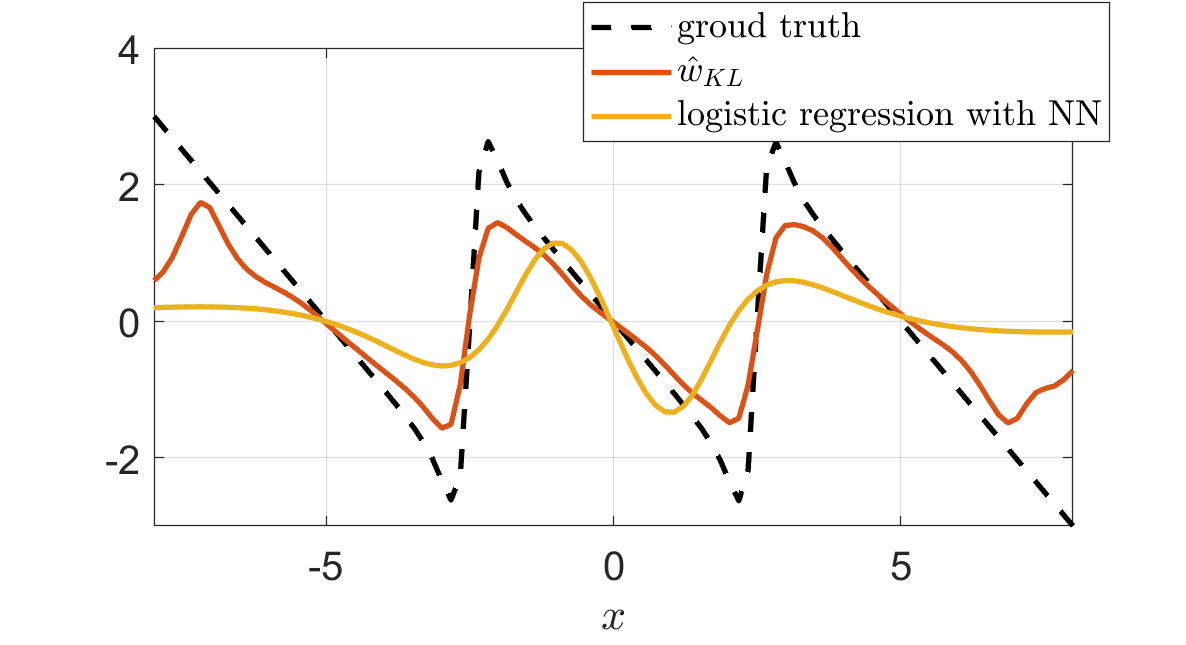
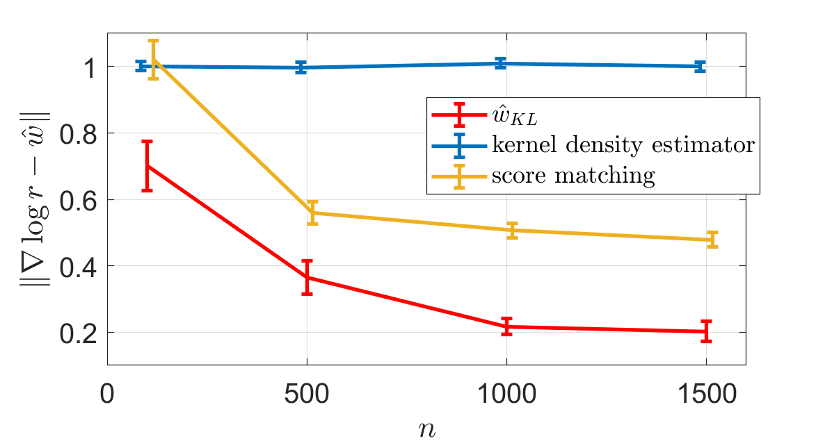
Figure 8: Left: $\nabla\log r({\boldsymbol{x}})$ and its approximations. Right: Estimation error with standard error.

Now we investigate the performance of estimating $\nabla\log r({\boldsymbol{x}})$ using the proposed gradient estimator and an indirect estimator using logistic regression. For the indirect estimator, we first train a Multilayer Perceptron (MLP) using a binary logistic regression to approximate $\log r$. Then obtain $\nabla\log r$ by auto-differentiating the estimated log ratio. The kernel bandwidth in our method is tuned by using the model selection criterion described in Section 4.4.

To conduct the experiments, we let $p=\mathcal{N}(-5,.5)/3+\mathcal{N}(0,.5)/3+\mathcal{N}(5,.5)/3$ and $q=\mathcal{N}(-5,1)/3+\mathcal{N}(0,1)/3+\mathcal{N}(5,1)/3$. From each distribution, 5000 samples are generated for approximating the gradients.

The left plot in Figure 8 shows the true gradient and its approximations. It can be seen that the direct gradient estimation is more accurate than estimating the log ratio first then taking the gradient.

The right plot in Figure 8 displays the estimation errors of different methods, comparing the proposed method with Kernel Density Estimation (KDE) and score matching, all applied to the same distributions in the previous experiment. KDE was previously used in approximating WGF (Wang et al., 2022). It first estimates $p$ and $q$ with $\hat{p}$ and $\hat{q}$ separately using non-parametric kernel density estimators, then approximates $\nabla\log r$ with $\nabla\log\hat{p}-\nabla\log\hat{q}$ . The score matching approximates $\nabla\log\hat{p}$ and $\nabla\log\hat{q}$ with the minimizers of Fisher-divergence. It has also been used in simulating particle ODEs in a previous work (Maoutsa et al., 2020). The estimation error plot shows that the proposed estimator yields more accurate results compared to the other two kernel-based gradient estimation methods, namely KDE and score matching.

O.2 Generative Sampling using WGF

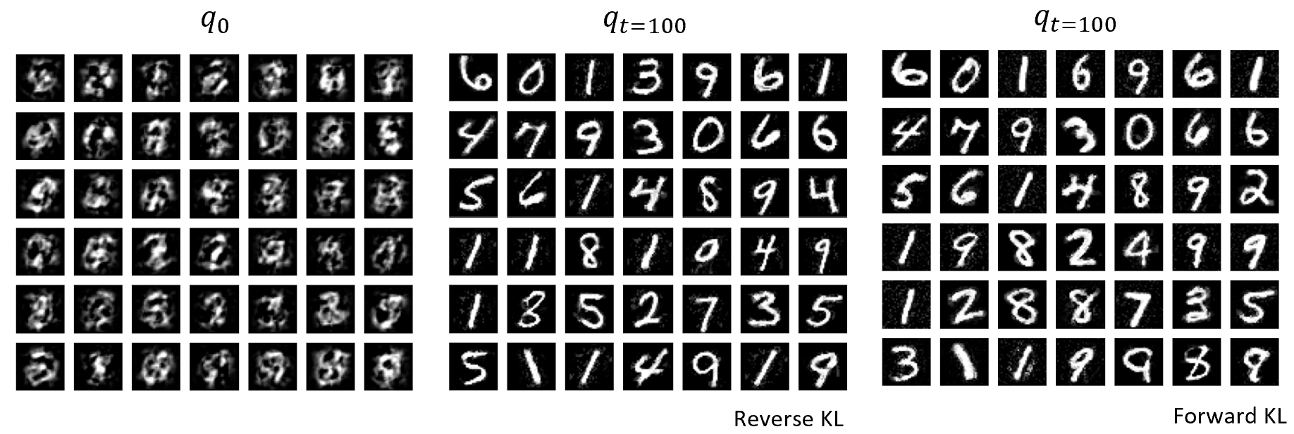
Figure 9: Samples generated using forward and backward KL velocity field.

In this experiment, we test the performance of the proposed gradient estimators by generating samples from a high dimensional target distribution (MNIST handwritten digits). We will check whether the quality of the particles can be improved by performing WGC using our estimated updates. Note that we do not intend to compare the generated samples with NN-based approaches, as the focus of our paper is on local estimation using kernel functions. We perform two different WGFs, forward KL and backward KL whose updates are approximated using $\hat{{\boldsymbol{w}}}_{\rightarrow}$ and $\hat{{\boldsymbol{w}}}_{\leftarrow}$ respectively. We let the initial particle distribution $q_{0}$ be $\mathcal{N}({\boldsymbol{\mu}},{\boldsymbol{\Sigma}})$, where ${\boldsymbol{\mu}},{\boldsymbol{\Sigma}}$ are the mean and covariance of the target dataset and fix the kernel bandwidth using “the median trick” (see the appendix for details).

The generated samples together with samples from the initial distribution $q_{0}$ are shown in Figure 9. Judging from the generated sample quality, it can be seen that both VGDs perform well and both have made significant improvements from the initial samples drawn from $q_{0}$.

We also provide two videos showing the animation of the first 100 gradient steps:

• Forward KL: https://youtube.com/shorts/HZcvUykrpbc

• Backward KL: https://youtube.com/shorts/AgN6dsDecCM

O.3 Feature Space Wasserstein Gradient Flow

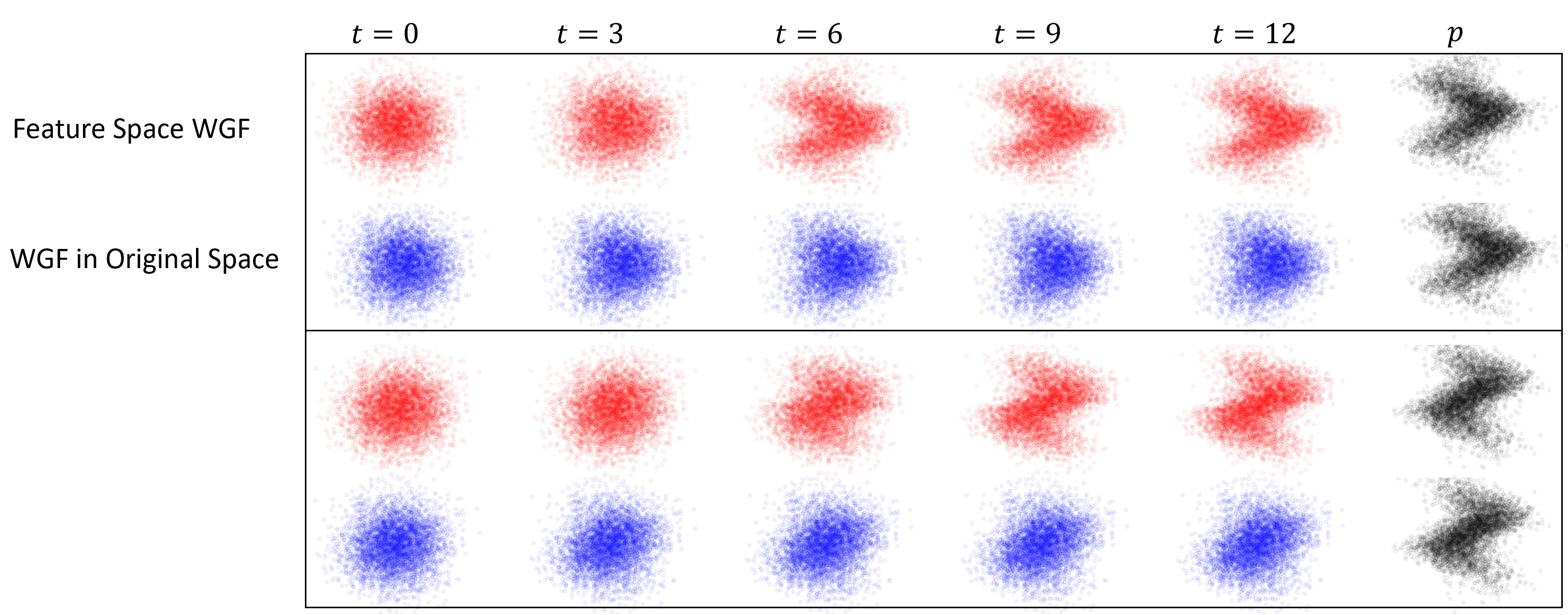
Figure 10: $\{{\boldsymbol{x}}_{q_{t}}\}$ in the first two dimensions $x_{1},x_{2}$. Feature space WGF converges in fewer steps compared to WGF in the original space. Above: $g=\cos$. Below: $g=\sin$.

In this experiment, we run WGF in a 5-dimensional space. The target distribution is

$$p=p_{12}({\boldsymbol{x}}_{1,2})p_{345}({\boldsymbol{x}}_{3,4,5}),p_{345}:=\mathcal{N}({\boldsymbol{0}},{\boldsymbol{I}})$$

and $p_{12}$ is constructed by a generative process. We generate samples in the first two dimensions as follows

$$X_{1}=g(X_{2})+\epsilon,X_{2}\sim\mathcal{N}(0,1),\epsilon\sim\mathcal{N}(0,1).$$

In our experiment, we draw 5000 samples from $p$, and 5000 samples from $q_{0}:=\mathcal{N}({\boldsymbol{0}},{\boldsymbol{I}})$, and run the backward KL gradient flow. Clearly, this WGF has a low dimensional structure since $p$ and $q$ only differs in the first two dimensions. We also run feature space backward KL field whose updates are calculated using (25). The feature function ${\boldsymbol{s}}({\boldsymbol{x}})={\boldsymbol{S}}^{\top}{\boldsymbol{x}}$ is learned by Algorithm 1.

The resulting particle evolution for both processes is plotted in Figure 10. For visualization purposes, we only plot the first two dimensions. It can be seen that the particles converge much faster when we explicitly exploit the subspace structure using the feature space WGF. In comparison, running WGF in the original space converges at a much slower speed.

In this experiments, we set the learning rates for both WGF and feature space WGF to be 0.1 and the kernel bandwidth $\sigma$ in our local estimators is tuned using cross validation with a candidate set ranging from 0.1 to 2.

References

• Ambrosio etΒ al. (2005) L.Β Ambrosio, N.Β Gigli, and G.Β SavarΓ©. Gradient flows: in metric spaces and in the space of probability measures. Springer Science & Business Media, 2005.
• Ansari etΒ al. (2021) A.Β F. Ansari, M.Β L. Ang, and H.Β Soh. Refining deep generative models via discriminator gradient flow. In International Conference on Learning Representations (ICLR 2021), 2021.
• Blei etΒ al. (2017) D.Β M. Blei, A.Β Kucukelbir, and J.Β D. McAuliffe. Variational inference: A review for statisticians. Journal of the American Statistical Association, 112(518):859–877, 2017.
• Chewi etΒ al. (2020) S.Β Chewi, T.Β LeΒ Gouic, C.Β Lu, T.Β Maunu, and P.Β Rigollet. Svgd as a kernelized wasserstein gradient flow of the chi-squared divergence. In Advances in Neural Information Processing Systems (NeurIPS 2020), volumeΒ 33, pages 2098–2109, 2020.
• Courty etΒ al. (2017a) N.Β Courty, R.Β Flamary, A.Β Habrard, and A.Β Rakotomamonjy. Joint distribution optimal transportation for domain adaptation. In Advances in Neural Information Processing Systems (NeurIPS 2017), volumeΒ 30, 2017a.
• Courty etΒ al. (2017b) N.Β Courty, R.Β Flamary, D.Β Tuia, and A.Β Rakotomamonjy. Optimal transport for domain adaptation. IEEE Transactions on Pattern Analysis and Machine Intelligence, 39(9):1853–1865, 2017b.
• Donders etΒ al. (2006) A.Β R.Β T. Donders, G.Β J.M.G. van der Heijden, T.Β Stijnen, and K.Β G.M. Moons. Review: A gentle introduction to imputation of missing values. Journal of Clinical Epidemiology, 59(10):1087–1091, 2006.
• Donsker and Varadhan (1976) M.Β D. Donsker and S.Β R.Β S. Varadhan. Asymptotic evaluation of certain markov process expectations for large timeβ€”iii. Communications on Pure and Applied Mathematics, 29(4):389–461, 1976.
• Fan (1993) J.Β Fan. Local Linear Regression Smoothers and Their Minimax Efficiencies. The Annals of Statistics, 21(1):196 – 216, 1993.
• Gao etΒ al. (2019) Y.Β Gao, Y.Β Jiao, Y.Β Wang, Y.Β Wang, C.Β Yang, and S.Β Zhang. Deep generative learning via variational gradient flow. In International Conference on Machine Learning (ICML 2019), pages 2093–2101, 2019.
• Gasser and MΓΌller (1979) T.Β Gasser and H-G MΓΌller. Kernel estimation of regression functions. In T.Β Gasser and M.Β Rosenblatt, editors, Smoothing Techniques for Curve Estimation, pages 23–68, Berlin, Heidelberg, 1979. Springer Berlin Heidelberg.
• Hastie etΒ al. (2001) T.Β Hastie, R.Β Tibshirani, and J.Β Friedman. The Elements of Statistical Learning: Data Mining, Inference, and Prediction. Springer, 2001.
• HyvΓ€rinen (2005) A.Β HyvΓ€rinen. Estimation of non-normalized statistical models by score matching. Journal of Machine Learning Research, 6:695–709, 2005.
• HyvΓ€rinen (2007) A.Β HyvΓ€rinen. Some extensions of score matching. Computational statistics & data analysis, 51(5):2499–2512, 2007.
• Kingma and Ba (2015) D.Β P. Kingma and J.Β Ba. Adam: A method for stochastic optimization. In International Conference on Learning Representations (ICLR 2015), 2015.
• Liu (2017) Q.Β Liu. Stein variational gradient descent as gradient flow. In Advances in Neural Information Processing Systems (NeurIPS 2017), volumeΒ 30, pages 3118–3126, 2017.
• Liu and Wang (2016) Q.Β Liu and D.Β Wang. Stein variational gradient descent: A general purpose bayesian inference algorithm. In Advances In Neural Information Processing Systems (NeurIPS 2016), volumeΒ 29, pages 2378–2386, 2016.
• Maoutsa etΒ al. (2020) D.Β Maoutsa, S.Β Reich, and M.Β Opper. Interacting particle solutions of fokker–planck equations through gradient–log–density estimation. Entropy, 22(8):802, 2020.
• Muzellec etΒ al. (2020) B.Β Muzellec, J.Β Josse, C.Β Boyer, and M.Β Cuturi. Missing data imputation using optimal transport. In International Conference on Machine Learning (ICML 2020), pages 7130–7140, 2020.
• Nadaraya (1964) E.Β A. Nadaraya. On estimating regression. Theory of Probability & Its Applications, 9(1):141–142, 1964.
• Nguyen etΒ al. (2010) X.Β Nguyen, M.Β J. Wainwright, and M.Β I. Jordan. Estimating divergence functionals and the likelihood ratio by convex risk minimization. IEEE Transactions on Information Theory, 56(11):5847–5861, 2010.
• Nowozin etΒ al. (2016) S.Β Nowozin, B.Β Cseke, and R.Β Tomioka. f-gan: Training generative neural samplers using variational divergence minimization. In Advances in Neural Information Processing Systems (NeurIPS 2016), volumeΒ 29, 2016.
• Scott (1991) D.Β W. Scott. Feasibility of multivariate density estimates. Biometrika, 78(1):197–205, 1991.
• Simons etΒ al. (2021) J.Β Simons, S.Β Liu, and M.Β Beaumont. Variational likelihood-free gradient descent. In Fourth Symposium on Advances in Approximate Bayesian Inference (AABI 2021), 2021.
• Song etΒ al. (2020) Y.Β Song, S.Β Garg, J.Β Shi, and S.Β Ermon. Sliced score matching: A scalable approach to density and score estimation. In Uncertainty in Artificial Intelligence (UAI 2020), pages 574–584, 2020.
• Sugiyama etΒ al. (2012) M.Β Sugiyama, T.Β Suzuki, and T.Β Kanamori. Density Ratio Estimation in Machine Learning. Cambridge University Press, 2012.
• Vincent (2011) P.Β Vincent. A connection between score matching and denoising autoencoders. Neural computation, 23(7):1661–1674, 2011.
• Wainwright (2019) M.Β J. Wainwright. High-Dimensional Statistics: A Non-Asymptotic Viewpoint. Cambridge University Press, 2019.
• Wang etΒ al. (2022) Y.Β Wang, P.Β Chen, and W.Β Li. Projected wasserstein gradient descent for high-dimensional bayesian inference. SIAM/ASA Journal on Uncertainty Quantification, 10(4):1513–1532, 2022.
• Wasserman (2010) L.Β Wasserman. All of Statistics: A Concise Course in Statistical Inference. Springer Publishing Company, Incorporated, 2010.
• Watson (1964) G.Β S. Watson. Smooth regression analysis. Sankhyā: The Indian Journal of Statistics, Series A (1961-2002), 26(4):359–372, 1964.
• Wibisono (2018) A.Β Wibisono. Sampling as optimization in the space of measures: The langevin dynamics as a composite optimization problem. In Conference on Learning Theory, pages 2093–3027, 2018.
• Yi etΒ al. (2023) M.Β Yi, Z.Β Zhu, and S.Β Liu. Monoflow: Rethinking divergence gans via the perspective of wasserstein gradient flows. In International Conference on Machine Learning (ICML 2023), pages 39984–40000, 2023.
• Yoon etΒ al. (2018) J.Β Yoon, J.Β Jordon, and M.Β Schaar. Gain: Missing data imputation using generative adversarial nets. In International conference on machine learning (ICML 2018), pages 5689–5698, 2018.
• Yu etΒ al. (2021) Q.Β Yu, A.Β Hashimoto, and Y.Β Ushiku. Divergence optimization for noisy universal domain adaptation. In Proceedings of the IEEE/CVF conference on computer vision and pattern recognition (CVPR 2021), pages 2515–2524, 2021.
• Zwitter and Soklic (1988) M.Β Zwitter and M.Β Soklic. Breast Cancer. UCI Machine Learning Repository, 1988.