PCA-aided calibration of systems comprising multiple unbiased sensors

Abstract

The calibration of sensors comprising inertial measurement units is crucial for reliable and accurate navigation. Such calibration is usually performed with specialized expensive rotary tables or requires sophisticated signal processing based on iterative minimization of nonlinear functions, which is prone to get stuck at local minima. We propose a novel calibration algorithm based on principal component analysis. The algorithm results in a closed-form formula for the sensor sensitivity axes and scale factors. We illustrate the proposed algorithm with simulation experiments, in which we assess the calibration accuracy in the case of calibration of a system consisting of 12 single-axis gyroscopes.

I Introduction

Accelerometers and gyroscopes are commonly known as inertial sensors. Inertial measurement units typically consist of multiple such sensors and are often augmented by magnetometers to estimate the inclination better. Before the navigation system is used, it must be calibrated. It is especially vital for sensors produced in micro-electrical-mechanical systems (MEMS) technology. Such sensors are generally delivered uncalibrated [1] to reduce the production costs of IMUs for mass-market products. There are two predominant classes of methods for IMU sensor calibration. One is based on expensive specialized equipment, such as precise mechanical platforms [2] or optical tracking systems (e.g., [3]). The other class, called multi-position calibration, relies on the measurements carried out under static conditions, which utilizes the knowledge of the magnitude of the measured vector quantity, such as the Earth’s gravity, e.g., [4, 5]. To the best of our knowledge, the methods that fall into the latter class require nonlinear optimization realized by iterative algorithms, e.g., Gauss-Newton algorithm [6], Newton-Raphson [4], Levenberg-Marquadt algorithm [1], or other algorithms provided by numerical toolboxes [5]. Our study falls into multi-position calibration as well. However, we propose measurement signal processing that leads to a closed form for the calibration parameters. We consider systems that consist of $m$ single-axis sensors, each of which measures the projection of a given vector-valued quantity onto the sensor sensitive axis. Such systems may consist of, e.g., accelerometers, gyroscopes, or magnetometers. We assume the following sensor measurement model

$$m_{ij}=\bm{a}_{i}^{T}\bm{v}_{j}+\eta_{ij},\quad i=1,\,\dots,\,m,\quad j=1,\,\dots,\,n,$$ (1)

where $m_{ij}$ is the read-out of $i$-th sensor, $\bm{v}_{j}\in\mathbf{R}^{d}$ is the measured vector quantity at $j$-th position of the system, $\bm{a}_{i}\in\mathbf{R}^{d}$ is a vector that encodes the scale and the sensitive axis of the sensor, and $\eta_{ij}$ is the Gaussian noise with zero mean. In our study, we treat dimension $d$ as an arbitrary positive integer. In practice, two values of $d$ are predominant, i.e., $d=3$ for the case of $3$-dimensional state space, and $d=2$ for the state space that takes the form of a plane. The absence of bias terms in (1) may be an inherent property of the system’s sensors, It can also result from bias estimation during a pre-calibration procedure, see Section IV. We assume that the measured quantity stays constant in magnitude for all $n$ positions of the considered system, i.e.,

$$\|\bm{v}_{j}\|=c,\quad j=1,\,\dots,\,n,$$ (2)

where $\|\bm{v}_{j}\|$ denotes the Euclidean norm of vector $\bm{v}_{j}$, and $c$ is an arbitrary scalar constant. Earth’s gravity or magnetic fields measured at a given point on Earth exemplify such quantities. The Angular rate of a rotary table that rotates with a fixed angular speed is another such quantity. In the former case, we may consider the calibration of a system consisting of accelerometers or magnetometers, and in the latter case — a system comprising gyroscopes.

The paper is organized as follows. The next section presents the main contribution of our study, i.e., the algorithm for finding the sensitive vectors of a sensor set. Section III discusses the number of positions required for the proposed calibration procedure. Section IV presents the results of numerical experiments, in which we have used the proposed algorithm to calibrate a system that consists of four triads of single-axis gyroscopes, see Fig. 1. Section V concludes our paper.

II Calibration procedure

Throughout the paper, we denote matrices with small bold letters with no subscript, e.g., $\bm{a}$, matrix columns with single-subscripted bold letters, e.g., $\bm{a}_{i}$, and matrix entries with regular double-subscripted letters, e.g. $a_{ij}$. Equation (1) takes the following form in the matrix notation.

$$\bm{m}=\bm{p}+\bm{\eta}=\bm{a}^{T}\bm{v}+\bm{\eta}.$$ (3)

II-A Noiseless case

Let us first consider the noiseless case, i.e., the case where $\bm{\eta}=\bm{0}$ in Eq. (3). Assume that matrix $\bm{p}$ is of the maximum possible rank, which is $d$. Thus, so are the ranks of matrices $\bm{a}$ and $\bm{v}$. Let vectors $\bm{e}_{1}$, …, $\bm{e}_{d}\in\mathbf{R}^{m}$ constitute a linear basis of the subspace $V\subset\mathbf{R}^{m}$ that is spanned by the columns of matrix $\bm{p}$, and let matrix $\bm{b}$ define the decomposition of matrix $\bm{p}$ columns in this basis, i.e.,

$$\bm{p}=\bm{a}^{T}\bm{v}=\bm{e}\bm{b}.$$ (4)

There must exist vectors $\bm{f}_{1}$, …, $\bm{f}_{d}\in\mathbf{R}^{d}$ such that

$$\bm{e}_{k}=\bm{a}^{T}\bm{f}_{k},\quad k=1,\,\dots,\,d.$$ (5)

By combining Eqs. (4) and (5) we get

$$\bm{v}=\bm{f}\bm{b}$$ (6)

and, in particular,

$$c^{2}=\|\bm{v}_{j}\|^{2}=\bm{b}_{j}^{T}\bm{f}^{T}\bm{f}\bm{b}_{j}=\bm{b}_{j}^{T}\bm{g}\bm{b}_{j},\quad j=1,\,\dots,\,n.$$ (7)

We may treat Eqs. (7) as a set of $n$ scalar equations for the entries of a symmetric matrix $\bm{g}=\bm{f}^{T}\bm{f}$. Once the equation set is solved for these entries, one may compute matrix $\bm{f}$ by eigendecomposition of $\bm{g}$:

$$\bm{g}=\bm{f}^{T}\bm{f}=\bm{q}^{T}\bm{\lambda}\bm{q},$$ (8)

and thus

$$\bm{f}=\bm{\lambda}^{\frac{1}{2}}\bm{q},$$ (9)

where $\bm{\lambda}$ is a diagonal matrix with non-negative entries, and $\bm{q}$ is an orthogonal matrix. By combining Eqs. (6) and (9)

$$\bm{v}=\bm{\lambda}^{\frac{1}{2}}\bm{q}\bm{b}.$$ (10)

Eventually, by substituting (10) into (4) and solving it for $\bm{a}$, we get

$$\bm{a}=\bm{\lambda}^{-\frac{1}{2}}\bm{q}\bm{e}^{T}.$$ (11)

The following algorithm concludes this subsection.

Algorithm 1.

Inputs: Noiseless sensor readings in the form of matrix $\bm{p}\in\mathbf{R}^{m\times n}$ of rank $d$, the magnitude $c$ of the measured vector quantity (see Eqs. (1)–(3)) Output: Matrices $\hat{\bm{v}}\in\mathbf{R}^{d\times n}$ and $\hat{\bm{a}}\in\mathbf{R}^{d\times m}$ such that $\bm{p}=\hat{\bm{a}}^{T}\hat{\bm{v}}$.

1. Choose an arbitrary linear basis $\bm{e}_{1}$, …, $\bm{e}_{d}$ for the subspace spanned by the columns of matrix $\bm{p}$ and decompose these columns relative to the basis:

   $$\bm{p}=\bm{e}\bm{b}.$$

2. Solve the following set of linear equations for the entries of symmetric matrix $\bm{g}\in\mathbf{R}^{d\times d}$:

   $$c^{2}=\bm{b}_{j}^{T}\bm{g}\bm{b}_{j},\quad j=1,\,\dots,\,n.$$

3. Compute the eigendecomposition of matrix $\bm{g}$:

   $$\bm{g}=\bm{q}^{T}\bm{\lambda}\bm{q}.$$

4. Compute $\hat{\bm{v}}=\bm{\lambda}^{\frac{1}{2}}\bm{q}\bm{b}$ and $\hat{\bm{a}}=\bm{\lambda}^{-\frac{1}{2}}\bm{q}\bm{e}^{T}$.

Remark 1.

If Eq. (7) has a unique solution $\bm{g}$, then columns of matrices $\hat{\bm{v}}$ and $\hat{\bm{a}}$ are determined uniquely up to an orthogonal transformation, i.e., they are equal to $\bm{v}$ and $\bm{a}$, respectively, up to the multiplication from the left by an arbitrary orthogonal matrix $\bm{r}\in\mathbf{R}^{d\times d}$. If Eq. (7) fails to have a unique solution $\bm{g}$, then the algorithm cannot recover the original matrix $\bm{v}$ from the readings even up to an orthogonal transformation.

Remark 2.

If constant $c$ is not known, then Algorithm 1 cannot determine the scale factors of sensors. However, by taking any value of $c$, e.g., $c=1$, we may at least reconstruct the sensors’ sensitive axes up to an orthogonal transformation, and find the scale factors of the sensors up to a common factor, provided that Eq. (7) has a unique solution.

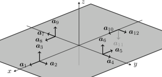
Figure 1: Sensitive vectors of four triads of gyroscopes considered in Section IV

II-B Noisy measurements

Due to the noise terms, matrix $\bm{m}$ of Eq. (3) is of the full rank, i.e., the probability of the rank of matrix $\bm{m}$ being full is $1$. Consequently, if the number of positions $n$ is bigger than the number of sensors $m$, then the columns of matrix $\bm{m}$ span the whole space $\mathbf{R}^{m}$. However, if the noise terms are small, the columns $\bm{m}_{j}$ treated as points in $\mathbf{R}^{m}$ must lie close to the subspace $V$ spanned by the columns of matrix $\bm{p}$. Therefore, we may estimate the subspace $V$ as a $d$-dimensional subspace $\hat{V}\subset\mathbf{R}^{m}$ that is the closest to the columns of matrix $\bm{m}$ in terms of the mean squared Euclidean distance. This task can be accomplished by Principal Component Analysis (PCA) method as presented in Pearson’s seminal paper [7]. If

$$\bm{t}=\bm{m}\bm{w},\quad\bm{w}\in\mathbf{R}^{m\times d}$$ (12)

is the PCA transformation of $\bm{m}$ truncated to the first $d$ principal axes, then the columns of matrix $\bm{t}$ span subspace $\hat{V}$. Before we follow the procedure introduced in the previous subsection, we need to approximate the columns of matrix $\bm{m}$ with those of matrix $\bm{t}$. Let us recall that the truncated PCA transformation can be obtained by truncated Singular Value Decomposition (SVD):

$$\bm{m}\approx\bm{u}\bm{s}\bm{w}^{T},\quad\bm{s}\in\mathbf{R}^{d\times d},$$ (13)

where the columns of matrices $\bm{u}\in\mathbf{R}^{n\times d}$ and $\bm{w}\in\mathbf{R}^{m\times d}$ are orthonormal, and $\bm{s}$ is a diagonal matrix. The truncated SVD gives

$$\bm{t}=\bm{m}\bm{w}=\bm{u}\bm{s}.$$ (14)

By Eckart-Young theorem [8], matrix $\hat{\bm{m}}=\bm{u}\bm{s}\bm{w}^{T}=\bm{t}\bm{w}^{T}$ is the best rank $d$ approximation to matrix $\bm{m}$ with respect to the Frobenius norm, i.e., the sum of squares of the entries of matrix $\bm{m}-\bm{x}$, where $\bm{x}$ is of rank $d$, attains its minimum at $\bm{x}=\hat{\bm{m}}$. Once we have approximated matrix $\bm{m}$ with rank $d$ matrix $\bm{t}\bm{w}^{T}$, we can recall the procedure presented in the previous subsection. Note that by having the SVD decomposition of matrix $\hat{\bm{m}}$:

$$\hat{\bm{m}}=\underbrace{\bm{u}}_{\bm{e}}\underbrace{\bm{s}\bm{w}^{T}}_{\bm{b}},$$ (15)

we can compute the analog of Eq. (4) by taking $\bm{e}=\bm{u}$ and $\bm{b}=\bm{s}\bm{w}^{T}$ as depicted in Eq. (15).

The following algorithm concludes this subsection.

Algorithm 2.

Inputs: Sensor readings in the form of matrix $\bm{m}\in\mathbf{R}^{m\times n}$, the length $c$ of vectors $\bm{v}_{j}$ (see Eqs. (1)–(3)) Output: Matrices $\hat{\bm{v}}\in\mathbf{R}^{d\times n}$ and $\hat{\bm{a}}\in\mathbf{R}^{d\times m}$ that, by the product $\hat{\bm{a}}^{T}\hat{\bm{v}}$, form the best rank $d$ approximation to matrix $\bm{m}$.

1. Compute truncated SVD of rank $d$ for matrix $\bm{m}$:

   $$\bm{m}\approx\bm{u}\bm{s}\bm{w}^{T}$$

2. Solve the following set of linear equations for the entries of symmetric matrix $\bm{g}\in\mathbf{R}^{d\times d}$:

   $$c^{2}=\bm{b}_{j}^{T}\bm{g}\bm{b}_{j},\quad j=1,\,\dots,\,n,$$

   where $\bm{b}_{j}$ are the columns of matrix $\bm{b}=\bm{s}\bm{w}^{T}$,

3. Compute the eigendecomposition of matrix $\bm{g}$:

   $$\bm{g}=\bm{q}^{T}\bm{\lambda}\bm{q}.$$

4. Compute $\hat{\bm{v}}=\bm{\lambda}^{\frac{1}{2}}\bm{q}\bm{b}$ and $\hat{\bm{a}}=\bm{\lambda}^{-\frac{1}{2}}\bm{q}\bm{u}^{T}$.

Note that Algorithm 2 generalizes Algorithm 1, i.e., Algorithm 2 may also be used in the absence of noise. Also, Remarks 1 and 2 stay valid except for the necessary change of the corresponding equalities that hold up to an orthogonal transformation into approximate equalities $\hat{\bm{a}}\approx\bm{a}$ and $\hat{\bm{v}}\approx\bm{v}$.

Remark 3.

If the sensor readings are noisy and the system of equations in Step 2 of Algorithm 2 is overdetermined, then the solution referred to in that step is meant to be the least square solution.

Remark 4.

Algorithm 2 is robust to small divergence from the assumption on equal length of vectors $\bm{v}_{j}$, as the disparity between the lengths of the vectors can be considered as an extra noise that contributes to $\bm{\eta}$ in Eq. (3).

III The number of required measurements

As stated in Remark 1, Algorithm 1 reconstructs matrices $\bm{a}$ and $\bm{v}$ up to an orthogonal transformation, provided that Eq. (7) has a unique solution $\bm{g}$. The same holds for an approximate reconstruction in the case of Algorithm 2. Since matrix $\bm{g}\in\mathbf{R}^{d\times d}$ is symmetric, the number of linear equations required to specify the entries of $\bm{g}$ uniquely is $\frac{d(d+1)}{2}$. In other words, in order to reconstruct matrices $\bm{a}$ and $\bm{v}$ with Algorithms 1 or 2 the number of positions $n$ has to satisfy the following inequality

$$n\geq\frac{d(d+1)}{2}.$$ (16)

In this section, we show that this bound cannot be loosened in general, i.e., there exist cases in which no algorithm can reconstruct matrices $\bm{a}$ and $\bm{v}$ with a smaller number of measurement setups $n$.

The number of scalar measurements that form matrix $\bm{p}$ is $nm$. The given magnitude of vectors $\bm{v}_{i}$ results in $n$ extra scalar data. The number of unknown entries of matrices $\bm{a}$ and $\bm{v}$ is $d(n+m)$. These matrices are to be determined up to an orthogonal transformation of $\mathbf{R}^{d}$. The dimension of the group of such transformations of $\mathbf{R}^{d}$ is $\frac{d(d-1)}{2}$. Thus, for the desired reconstruction of $\bm{a}$ and $\bm{v}$, the following inequality must hold$nm+n\geq(m+n)d-\frac{d(d-1)}{2}.$ By rearranging this inequality, we get

$$\left(n-d\right)\left(m-d+1\right)\geq\frac{d(d-1)}{2}.$$ (17)

In particular, the number of setups $n$ hast to be greater than the dimension $d$, and the number of sensors $m$ must be at least $d$. Moreover, for the minimal number of sensors $m=d$, Inequality (17) results in (16). In particular, $n\geq 3$ for dimension $d=2$, and $n\geq 6$ for $d=3$.

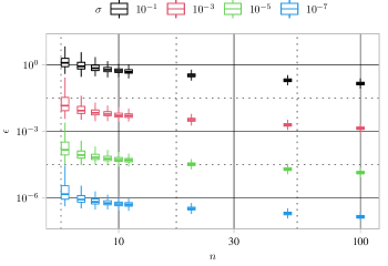
Figure 2: Calibration error of four triads of gyroscopes

IV Calibration of multiple gyroscopes

Gyroscopes are often produced in presumably orthonormal triads. Multiple instances of such triads can be used to reduce measurement errors after data fusion [9]. We have considered a system of four gyroscope triads in the configuration shown in Fig. 1, i.e., with sensitive vectors of the gyroscopes constituting the following matrix:

$$\bm{a}_{\text{model}}=\setcounter{MaxMatrixCols}{12}\begin{pmatrix}1&0&0&0&1&0&0&-1&0&1&0&0\\ 0&1&0&-1&0&0&1&0&0&0&0&-1\\ 0&0&1&0&0&1&0&0&1&0&1&0\end{pmatrix}.$$

Such a system needs calibration because of the internal sensitive-axes misalignment, scale factor spread between sensors comprising every single triad, and the finite precision of the multi-triad assembly. One may perform the needed calibration with the help of a rotary table that can turn with a known angular rate. We propose the following measurements for each of $n$ different positions of the system on the table.

1. Place the system in the $i$-th position on the steady rotary table and record the reading of the sensors. The time-averaged readings $\bm{b}_{i}^{\prime}$ are used as the estimates for the biases of the gyroscopes.

2. Switch on the rotary table and wait until it rotates steadily.

3. Record and time-average the readings of the sensors to form vectors $\bm{m}_{i}^{\prime}$.

We remove the measurement bias by subtracting the steady-state read-outs from the readings obtained during the rotary movement, i.e., we set

$$\bm{m}_{i}=\bm{m}_{i}^{\prime}-\bm{b}_{i}^{\prime}.$$ (18)

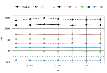
Figure 3: Calibration error statistics (for four triads of gyroscopes) as functions of the standard deviation $\sigma$ of the measurement noise

To simulate a real scenario, we assumed that each of the sensor sensitivity axes, represented by columns of matrix $\bm{a}$, differ from the columns of $\bm{a}_{\text{model}}$ by a random Gaussian vector with zero mean and diagonal covariance matrix with $\sigma=0.01$ on the diagonal. We picked at random $n$ different positions (orientations) of the system and simulated the sensors readings according to Eq. (3). Then, we invoked Algorithm 2 to compute the matrix $\hat{\bm{a}}$ of sensitive vectors of the gyroscopes. Matrix $\hat{\bm{a}}$ is expected to approximate $\bm{a}$ up to an orthogonal transformation. Therefore, to compare these matrices, we first find two orthogonal matrices $\bm{h}$ and $\bm{k}$ such that $\bm{h}\bm{a}$ and $\bm{k}\hat{\bm{a}}$ are upper-triangular with positive entries on the main diagonal. Then, we compute the calibration error $\epsilon$, which we define as the Frobenius norm of matrix $\bm{h}\bm{a}-\bm{k}\hat{\bm{a}}$, i.e.,

$$\epsilon=\|\bm{h}\bm{a}-\bm{k}\hat{\bm{a}}\|_{F},$$ (19)

where $\|\bm{x}\|_{F}$ denotes the square root of the sum of squares of the entries of matrix $\bm{x}$. For each of the considered values of $n$ and noise standard deviation $\sigma$, we have repeated the simulation of the calibration procedure $1000$ times to assess its statistical behavior. Fig. 2 shows the boxplot of the calibration error. The line plots of Fig. 3 indicate that the median and the interquartile range of the calibration error are approximately proportional to the standard deviation $\sigma$ of the measurement error. Figure 4 shows that these statistics drop with the number $n$ of measurements at the rate $n^{-0.5}$ approximately.

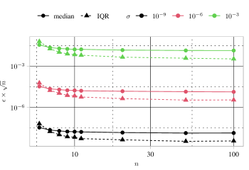
Figure 4: Calibration error statistics (for four triads of gyroscopes) as functions of the number of calibration positions $n$

V Conclusion

We have proposed a novel method for calibrating multiple-sensor systems with the help of a constant magnitude vector quantity. The crucial merit of the method is the closed form for the computed parameters under calibration. The method requires the sensors to be unbiased or the sensor bias to be computed before applying the proposed calibration procedure. We have noted that the proposed algorithm allows for the calibration of the sensors up to an orthogonal transformation, provided the magnitude of the measured quantity is known. In the opposite case, the calibration procedure leaves a common scale factor unresolved. We have deduced the minimum number of positions needed to complete the calibration with the above-specified degree of ambiguity. The proposed calibration method accuracy depends on the number of considered positions and the measurement noise level. The results of the conducted numerical experiments indicate that the calibration error is linearly proportional to the standard deviation of measurement errors and inversely proportional to the square of the number of positions.

References

- [1] M. Sipos, P. Paces, J. Rohac, and P. Novacek, “Analyses of triaxial accelerometer calibration algorithms,” IEEE Sensors Journal, vol. 12, no. 5, pp. 1157–1165, 2012.
- [2] D. Titterton, J. L. Weston, and J. Weston, Strapdown inertial navigation technology. IET, 2004, vol. 17.
- [3] H. Wei, T. Zhang, and L. Zhang, “A fast analytical two-stage initial-parameters estimation method for monocular-inertial navigation,” IEEE Transactions on Instrumentation and Measurement, vol. 71, pp. 1–12, 2022.
- [4] J.-O. Nilsson, I. Skog, and P. Händel, “Aligning the forces—eliminating the misalignments in imu arrays,” IEEE Transactions on Instrumentation and Measurement, vol. 63, no. 10, pp. 2498–2500, 2014.
- [5] J. Rohac, M. Sipos, and J. Simanek, “Calibration of low-cost triaxial inertial sensors,” IEEE Instrumentation & Measurement Magazine, vol. 18, no. 6, pp. 32–38, 2015.
- [6] I. Skog and P. Händel, “Calibration of a MEMS inertial measurement unit,” in XVII IMEKO world congress, 2006, pp. 1–6.
- [7] K. Pearson, “LIII. On lines and planes of closest fit to systems of points in space,” The London, Edinburgh, and Dublin Philosophical Magazine and Journal of Science, vol. 2, no. 11, pp. 559–572, 1901.
- [8] C. Eckart and G. Young, “The approximation of one matrix by another of lower rank,” Psychometrika, vol. 1, no. 3, pp. 211–218, Sep. 1936.
- [9] L. Wang, H. Tang, T. Zhang, Q. Chen, J. Shi, and X. Niu, “Improving the navigation performance of the mems imu array by precise calibration,” IEEE Sensors Journal, vol. 21, no. 22, pp. 26 050–26 058, 2021.