TOI-1130: A photodynamical analysis of a hot Jupiter in resonance with an inner low-mass planet

The TOI-1130 is a known planetary system around a K-dwarf consisting of a gas giant planet, TOI-1130 c, on an 8.4-day orbit, accompanied by an inner Neptune-sized planet, TOI-1130 b, with an orbital period of 4.1 days. We collected precise radial velocity (RV) measurements of TOI-1130 with the HARPS and PFS spectrographs as part of our ongoing RV follow-up program. We perform a photodynamical modeling of the HARPS and PFS RVs, and transit photometry from the Transiting Exoplanet Survey Satellite (TESS) and the TESS Follow-up Observing Program. We determine the planet masses and radii of TOI-1130 b and TOI-1130 c to be $M_{\mathrm{b}}\,=19.28\pm\,0.97$ $M_{\oplus}$ and $R_{\mathrm{b}}\,=3.56\pm\,0.13$ $R_{\oplus}$, and $M_{\mathrm{c}}\,=325.59\pm\,5.59$ $M_{\oplus}$ and $R_{\mathrm{c}}\,=13.32^{+1.55}_{-1.41}$ $R_{\oplus}$, respectively. We spectroscopically confirm TOI-1130 b that was previously only validated. We find that the two planets orbit with small eccentricities in a 2:1 resonant configuration. This is the first known system with a hot Jupiter and an inner lower mass planet locked in a mean-motion resonance. TOI-1130 belongs to the small yet increasing population of hot Jupiters with an inner low-mass planet that challenges the pathway for hot Jupiter formation. We also detect a linear RV trend possibly due to the presence of an outer massive companion.

1 Introduction

The diversity within the exoplanet “jungle” is one of the astonishing outcomes in exoplanet research over the last 30 years. Exoplanets are found to survive in hostile environments in orbits with very short orbital periods. The first exoplanet detected around the solar-like star 51 Peg (Mayor & Queloz 1995), represents one of these new types of planets, a gas giant on a short-period orbit ($P_{\mathrm{orb}}<10$ day), also known as a hot Jupiter. Even 27 years after this discovery, there is no clear picture of their formation, whether they formed in situ or further out beyond the ice line and migrated inwards (see Fortney et al. (2021) and references therein).

The in situ formation mechanism is proposed to happen at the present-day close-in orbit when a core accretes gas from the gaseous protoplanetary disks (Boley et al. 2016; Bailey & Batygin 2018). If sufficient material is available close to the star to build up a $\sim$ 10 $M_{\oplus}$ core (Rafikov 2006), and the other conditions, such as planetesimal accretion luminosity and gas opacity, are right (Lee et al. 2014), the core will accrete gas as long as the gaseous protoplanetary disk is not dissipated, and form a gas giant (Dawson & Johnson 2018). In the migration theory, it is assumed that all gas giants form beyond the ice-line (Dodson-Robinson et al. 2009), and some of them migrate close to the host star to become hot Jupiters (Dawson & Johnson 2018). This migration is thought to happen either through the interaction with the gas disk during the formation period (Lin et al. 1996; Nelson & Papaloizou 2004; Kley & Nelson 2012; Bitsch et al. 2019), or via high-eccentricity migration (HEM; Rasio & Ford 1996; Mustill et al. 2015) at a later stage. In the HEM scenario the eccentricities are either excited by planet–planet scattering (Rasio & Ford 1996; Chatterjee et al. 2008), by the Kozai–Lidov cycles (Wu & Murray 2003), or by interactions with a companion (Wu & Lithwick 2011; Petrovich 2015). Recent discoveries suggest that HEM is the dominant mechanism (Vick et al. 2019, 2023; Jackson et al. 2023).

Hot Jupiters are often accompanied by gas giants on wider orbits (Knutson et al. 2014) but rarely accompanied by aligned nearby planets (Steffen et al. 2012; Huang et al. 2016; Hord et al. 2021; Ivshina & Winn 2022). The absence of low-mass planets in systems containing a hot Jupiter is one of the key arguments in support of HEM over the in situ formation.

However, systems have been detected in which a hot gas giant is accompanied by an inner low-mass planet. The first example is WASP-47 (Hellier et al. 2012; Becker et al. 2015; Bryant & Bayliss 2022; Nascimbeni et al. 2023). Since then, more systems have been detected: Kepler-730 (Zhu et al. 2018; Cañas et al. 2019), TOI-2000 (Sha et al. 2022), WASP-132 (Hellier et al. 2017; Hord et al. 2022), and TOI-1130 (Huang et al. 2020a), that we discuss here in more detail. Moreover, there is some indication from transit timing variation (TTV; Agol et al. 2005) measurements that non-aligned nearby companions to hot Jupiters may be more common than previously thought, although more work is needed to expand the sample size (Wu et al. 2023). Those systems rule out HEM, which allows the formation of outer companions and prohibits the formation of inner companions. Instead, those systems could have formed through disk migration (Mandell & Sigurdsson 2003; Fogg & Nelson 2005, 2007; Ogihara et al. 2014) or in situ (Poon et al. 2021), since both scenarios allow the formation of terrestrial planets inside the orbit of a hot Jupiter. Compared to the other systems that contain a hot Jupiter and an inner low-mass planet, TOI-1130 shows a unique orbital configuration: their orbital periods are close to a 2:1 period commensurability indicating that this system could be in a first-order mean motion resonance (MMR). If confirmed TOI-1130 would have formed most likely via disk migration (Mustill & Wyatt 2011; Pichierri et al. 2018) and not via in situ formation. Thus, we can distinguish between different formation scenarios by knowing the system’s architecture. In situ formation permits the formation of nearby planets, disk migration permits the formation of nearby planets in resonant orbits, and HEM permits the formation of outer planets.

In this article, we present a study of the architecture of TOI-1130, a system that contains a gas giant (TOI-1130 c) and a lower mass planet (TOI-1130 b) detected by Huang et al. (2020a). We carried out spectroscopic ground-based follow-up of TOI-1130 to determine the planetary and orbital parameters, especially for the inner planet TOI-1130 b, which had previously only been validated. Since the orbital period ratio of the two planets is close to a 2:1 period commensurability, we expect to measure large TTVs as already reported in Huang et al. (2020a). Thus, we acquired photometric follow-up to have a good phase coverage of the expected TTV signal. The ground-based photometry is modeled photodynamically together with the Transiting Exoplanet Survey Satellite (TESS) and radial velocity (RV) data to determine precisely the orbital and planetary parameters.

2 Observation and data reduction

We here provide a brief description of the TOI-1130 observations and time-series data used in the subsequent analysis: the space-based TESS photometry (Sect. 2.1), the ground-based photometry (Sect. 2.2), and the high-resolution spectroscopy (Sect. 2.3).

2.1 TESS photometry

TOI-1130 was observed by TESS in Sectors 13 and 27 in the southern ecliptic hemisphere. Sector 13 was observed between 2019 Jul 18 and 19, covering six transits of TOI-1130 b and three transits of TOI-1130 c. Sector 27 was observed between 2020 Jul 5 and 30 spanning six transits of TOI-1130 b and three transits of TOI-1130 c. While TOI-1130 was observed in the 30-min cadence mode in Sector 13 (Camera 2, CCD 1), it was observed in Sector 27 with a higher cadence rates of 2-min and 20 s (Camera 1, CCD 1).

We used in the subsequent analysis the publicly available $\mathrm{KSPSAP\_FLUX}$ light curves produced by the MIT Quick-Look-Pipeline (QLP; Huang et al. 2020b, 2020c; Kunimoto et al. 2021) and the Presearch Data Conditioning (PDC) light curves (Smith et al. 2012; Stumpe et al. 2014) produced by the Science Processing Operations Center (SPOC; Jenkins et al. 2016) at NASA Ames Research Center downloaded from the Mikulski Archive for Space Telescopes for Sector 13 and Sector 27, respectively. We note that Huang et al. (2020a) based their study on their own photometry created for Sector 13.

2.2 Ground-based photometry

Table 1: Ground-based light curve observations of TOI-1130 b and TOI-1130 c.

Observatory	Aperture [m]	Location	UTC Date	Filter	Planet	Transit number
LCOGT-SSO	1.0	Siding Spring, Australia	2019-09-05	Pan-STARRS $z$-short	b	19
PEST	0.31	Perth, Australia	2019-10-01	$R_{c}$	c	13
LCOGT-SSO	1.0	Siding Spring, Australia	2020-05-05	Pan-STARRS $z$-short	c	39
LCOGT-SSO	1.0	Siding Spring, Australia	2020-05-05	$B$	c	39
LCOGT-SAAO	1.0	Sutherland, South Africa	2020-06-07	Pan-STARRS $z$-short	c	43
LCOGT-SAAO	1.0	Sutherland, South Africa	2020-06-07	Pan-STARRS $z$-short	c	43
LCOGT-SSO	1.0	Siding Spring, Australia	2020-08-05	Pan-STARRS $z$-short	c	50
El Sauce Observatory	0.36	Coquimbo Province, Chile	2020-08-22	$R_{c}$	c	52
PEST	0.31	Perth, Australia	2020-08-30	$R_{c}$	c	53
LCOGT-SAAO	1.0	Sutherland, South Africa	2021-04-12	Pan-STARRS $z$-short	c	80
LCOGT-SAAO	1.0	Sutherland, South Africa	2021-06-10	Sloan $i^{\prime}$	b	177
LCOGT-CTIO	1.0	Cerro Tololo, Chile	2021-06-19	Sloan $i^{\prime}$	b	179
LCOGT-CTIO	1.0	Cerro Tololo, Chile	2021-06-26	Sloan $i^{\prime}$	c	88
LCOGT-CTIO	1.0	Cerro Tololo, Chile	2021-06-27	Sloan $i^{\prime}$	c	88
LCOGT-SSO	1.0	Siding Spring, Australia	2021-07-30	Sloan $i^{\prime}$	c	93
LCOGT-SAAO	1.0	Sutherland, South Africa	2021-08-02	Sloan $i^{\prime}$	b	190
LCOGT-CTIO	1.0	Cerro Tololo, Chile	2021-08-06	Sloan $i^{\prime}$	b	191
LCOGT-SAAO	1.0	Sutherland, South Africa	2021-08-07	Sloan $i^{\prime}$	c	94
LCOGT-CTIO	1.0	Cerro Tololo, Chile	2021-08-10	Sloan $i^{\prime}$	b	192
ASTEP	0.4	East Antarctic plateau	2021-08-24	Similar to $R_{c}$	c	96

We acquired ground-based time-series photometry of TOI-1130 as part of the TESS Follow-up Observing Program (TFOP; Collins et al. 2018; Collins 2019). In addition to the photometry published in Huang et al. (2020a), we observed five transits of TOI-1130 b and 13 of TOI-1130 c as listed in Table 1. We used the TESS Transit Finder, which is a customized version of the Tapir software package (Jensen 2013), to schedule our transit observations.

We observed 16 transits using the Las Cumbres Observatory Global Telescope (LCOGT; Brown et al. 2013) 1.0-m network. The telescopes are equipped with $4096\times 4096$ Sinistro cameras having an image scale of $0\aas@@fstack{\prime\prime}389$ per pixel, resulting in a $26\arcmin\times 26\arcmin$ field of view. The images were calibrated by the standard LCOGT BANZAI pipeline (McCully et al. 2018), and photometric data were extracted using AstroImageJ (Collins et al. 2017).

We observed two transits from the Perth Exoplanet Survey Telescope (PEST) near Perth, Australia. The 0.3-m telescope is equipped with a $1530\times 1020$ SBIG ST-8XME camera with an image scale of 1$\aas@@fstack{\prime\prime}$2 pixel^-1, resulting in a $31\arcmin\times 21\arcmin$ field of view. A custom pipeline based on C-Munipack was used to calibrate the images and extract the differential photometry.

We observed one transit from the Evans 0.36-m telescope at El Sauce Observatory in Coquimbo Province, Chile. The telescope is equipped with a $1536\times 1024$ SBIG STT-1603-3 camera. The image scale is 1$\aas@@fstack{\prime\prime}$47 pixel^-1 with in-camera binning $2\times 2$, resulting in an $18.8\arcmin\times 12.5\arcmin$ field of view. The images were calibrated and photometric data were extracted using AstroImageJ.

The Antarctica Search for Transiting ExoPlanets (ASTEP) program on the East Antarctic plateau (Guillot et al. 2015; Mékarnia et al. 2016) also observed one transit. The 0.4-m telescope is equipped with an FLI Proline science camera with a KAF-16801E, $4096\times 4096$ front-illuminated CCD. The camera has an image scale of $0\aas@@fstack{\prime\prime}93$ pixel^-1 resulting in a $1^{\circ}\times 1^{\circ}$ corrected field of view. The data were processed using an automated IDL-based pipeline described in Abe et al. (2013).

2.3 High-resolution spectroscopy

We acquired 49 high-resolution ($R$ $\approx$ 115 000) spectra using the High Accuracy Radial velocity Planet Searcher (HARPS; Mayor et al. 2003) spectrograph mounted at the 3.6-m telescope of the European Southern Observatory (ESO), La Silla, Chile. The observations were performed between 2019 Sep 18 and 19 as part of ESO programs 1102.C-0923 (PI: Gandolfi), and 60.A-9709 (technical night). In total, we observed the target on 41 individual nights with exposure times of 35 minutes. We reduced the data using the HARPS data reduction software (DRS; Lovis & Pepe 2007) and extracted the radial velocity by cross-correlating the HARPS spectra with a K5 numerical mask (Baranne et al. 1996; Pepe et al. 2002) and achieved a mean precision of 1.1 m $\mathrm{s}^{-1}$. We also used the DRS to measure the Ca ii H & K lines and to calculate the S-index, and extracted the full width at half maximum (FWHM) and the bisector inverse slope (BIS) of the cross-correlation function (CCF). These values are listed in Table 4.

We also observed TOI-1130 with the Planet Finder Spectrograph (PFS; Crane et al. 2006, 2008, 2010), which is mounted on the 6.5-m Magellan II (Clay) Telescope at Las Campanas Observatory in Chile. PFS is a slit-fed echelle spectrograph with a wavelength coverage of $3910$–$7340$ Å. We used a 0.3″ slit and $1\times 2$ binning, which yields a resolving power of $R\approx 133\,000$. Wavelength calibration is achieved via an iodine gas cell, which also allows the characterization of the instrumental profile. We obtained 20 spectra, observed through iodine, between 2019 Sep 12 and Oct 12, leading to six individual observation nights with typical exposure times of 20 minutes for each exposure. The last observations covered nine spectra and were meant to encompass the transit of TOI-1130 b to detect the Rossiter–McLaughlin (RM) effect, but the observations missed the transit window due to TTVs. We also obtained an iodine-free template observation with an 80-minute exposure time. The radial velocities were extracted using a custom IDL pipeline following the prescriptions of Marcy & Butler (1992) and Butler & Marcy (1996), and achieved a mean precision of 1.4 m $\mathrm{s}^{-1}$. The velocities are presented in Table 5. Following the prescription of Butler et al. (2017), we also calculated the S-index, measured from the core emission of the Ca ii H & K lines, and the H-index, which measures the chromospheric emission component in the H$\alpha$ line. These values are also reported in Table 5.

3 Data analysis

The analysis is done in steps. First, we carry out stellar modeling of the spectra (Sect. 3.1 and 3.2). We take advantage of the high-resolution and high signal-to-noise ratio (S/N) of the co-added HARPS spectra to independently derive the fundamental stellar parameters. Second, we perform a periodogram analysis of the radial velocities (Sect. 3.3) to identify which signals are present in the RV time series. Third, we modeled the photometry (Sect. 3.4) to uncover the TTVs and extract the transit times used in the photodynamical analysis. Each previous step is required to carry out the photodynamical modeling of the photometry and RV measurements (Sect. 3.5) to determine the planet and orbital parameters.

3.1 Stellar modeling with iSpec

[b] Parameter Reference RA [^∘] 286.376006 1 Dec [^∘] -41.43764 1 Spectral type K6–K7 2 B [mag] 12.42 $\pm$ 0.26 3 V [mag] 11.59 $\pm$ 0.16 3 TESS [mag] 10.1429 $\pm$ 0.0061 4 Gaia [mag] 10.8989 $\pm$ 0.0028 1 J [mag] 9.055 $\pm$ 0.023 5 H [mag] 8.493 $\pm$ 0.059 5 K [mag] 8.351 $\pm$ 0.033 5 WISE 3.4 um [mag] 8.266 $\pm$ 0.022 6 WISE 4.6 um [mag] 8.339 $\pm$ 0.019 6 WISE 12 um [mag] 8.244 $\pm$ 0.024 6 WISE 22 um [mag] 8.472 $\pm$ 0.361 6 RUWE 1.14 1 Distance [pc] $58.41\pm 0.07$ 1 Age [Gyr] 3.2–5 this work Parameter iSpec & PARAM 1.5 VOSA $T_{\mathrm{eff}}$ [K] $4350\pm 60$ 4300–4400 [Fe/H][dex] $0.30\pm 0.06$ 0.0–0.5 $\log g$ [cm $\mathrm{s}^{-2}$] $4.62\pm 0.04$ 4–5 $v_{\mathrm{rot}}\sin{i_{\star}}$ [km $\mathrm{s}^{-1}$] $\leq$ 3 - $M_{\star}$ [$M_{\odot}$] $0.71\pm 0.02$ - $R_{\star}$ [$R_{\odot}$] $0.68\pm 0.02$ 0.66–0.74 $L_{\star}$ [$L_{\odot}$] - 0.148–0.154 (1) Gaia eDR3 (Gaia Collaboration et al. 2016; Gaia Collaboration et al. 2022; Babusiaux, C. et al. 2022); (2) Empirical spectral type-colour sequence (Pecaut & Mamajek 2013); (3) Tycho-2 catalogue (Høg et al. 2000); (4) TIC v8.2 (Paegert et al. 2022); (5) 2MASS (Cutri et al. 2003); (6) WISE (Cutri et al. 2021).

Table 2: Stellar parameters of TOI-1130.

We used the co-added high-resolution HARPS spectrum (S/N $\approx$ 300 per pixel at 5500 Å) to determine the spectroscopic parameters of TOI-1130 using the iSpec framework (Blanco-Cuaresma et al. 2014; Blanco-Cuaresma 2019). Specifically, we used the Spectroscopy Made Easy radiative transfer code (SME; Valenti & Piskunov 1996; Piskunov & Valenti 2017), the MARCS atmospheres models (Gustafsson et al. 2008), and the version 5 of the GES atomic line list (Heiter et al. 2015), embedded in the iSpec framework. The models allow for fitting the effective temperature $T_{\mathrm{eff}}$ between 2500–8000 K, surface gravity $\log g$ between 0.00–5.00 dex, and metallicity [Fe/H] between $-$5.00–1.00 dex. iSpec uses a nonlinear least-squares (Levenberg-Marquardt) fitting algorithm (Markwardt 2009) to minimize the $\chi^{2}$ value between the observed spectra and the computed synthetic ones based on these models. We fitted simultaneously for an effective temperature, surface gravity, metallicity, and the projected stellar equatorial velocity in the region between 480 and 680 nm. We used the empirical relations for the microturbulence and macroturbulence velocities ($V_{\rm mic}$, $V_{\rm mac}$) included in the iSpec framework to reduce the number of free parameters in our analysis. The spectral resolution was taken from spectrograph specifications. The effective temperature and metallicity derived in the iSpec analysis together with the Gaia eDR3 parallax and 2MASS J, H, K magnitudes were then put into the Bayesian parameter estimation code PARAM 1.5 (da Silva et al. 2006; Rodrigues et al. 2014, 2017). PARAM 1.5 uses the PARSEC isochrones (Bressan et al. 2012) to estimate stellar parameters, such as stellar mass, radius, age, and surface gravity. We found good agreement between surface gravity derived in iSpec, but with reduced uncertainty. PARAM 1.5 computes relative uncertainties assuming that the theoretical models represent reliable descriptions of stars. The whole procedure is described in da Silva et al. (2006).

3.2 SED analysis with VOSA

As a reality check, we also analyzed the spectral energy distribution (SED) with the Virtual Observatory SED Analyser (VOSA; Bayo et al. 2008). We compared the results from five different models: BT-NextGen GNS93 (Grevesse et al. 1993; Barber et al. 2006; Allard et al. 2012), BT-NextGen AGSS2009 (Barber et al. 2006; Asplund et al. 2009; Allard et al. 2012), BT-Settl-AGSS2009 (Barber et al. 2006; Asplund et al. 2009; Allard et al. 2012), BT-Settl-CIFIST (Barber et al. 2006; Caffau et al. 2011; Allard et al. 2012), and Coelho Synthetic stellar library (Coelho 2014) to estimate $T_{\mathrm{eff}}$, $\log g$, [Fe/H], and the interstellar extinction $A_{\mathrm{v}}$. We use coordinates and distances from Gaia eDR3 and set limits in our analysis to $T_{\mathrm{eff}}$ = 3000–6000 K, and $\log g$ = 4.0–5.0 dex based on the parameters derived in Section 3.1. We set the limit for [Fe/H] between $-$0.5 and 0.5 dex if possible; however, the BT-NextGen GNS93 enables metallicity only up to 0.3, the Coelho Synthetic stellar library up to 0.2, and the BT-Settl-CIFIST are available only for the solar metallicity. For our SED fitting, we use the Tycho (Høg et al. 2000), Gaia DR2 (Gaia Collaboration et al. 2018), Gaia eDR3 (Gaia Collaboration et al. 2021), 2MASS (Cutri et al. 2003), and WISE (Cutri et al. 2021) photometry.

VOSA performs the ${\chi}^{2}$ minimization procedure to compare theoretical models with the observed photometry. For each model, we take three results with the lowest ${\chi}^{2}$. The lowest and highest value of each parameter from these results is used to create the final intervals. Additionally, the stellar radius is derived via the Stefan–Boltzmann law.

We report the derived stellar parameters from the co-added HARPS spectra in Table 2.

3.3 Periodogram analysis of the HARPS data

We searched the radial velocity data for the Doppler reflex motions induced by the two transiting planets. To this end, we performed a periodogram analysis of the HARPS and PFS data as well as the activity indicators (Sect. 2.3), which also allowed us to search for the stellar rotational period and for possible additional Doppler signals that might be induced by the presence of other orbiting objects.

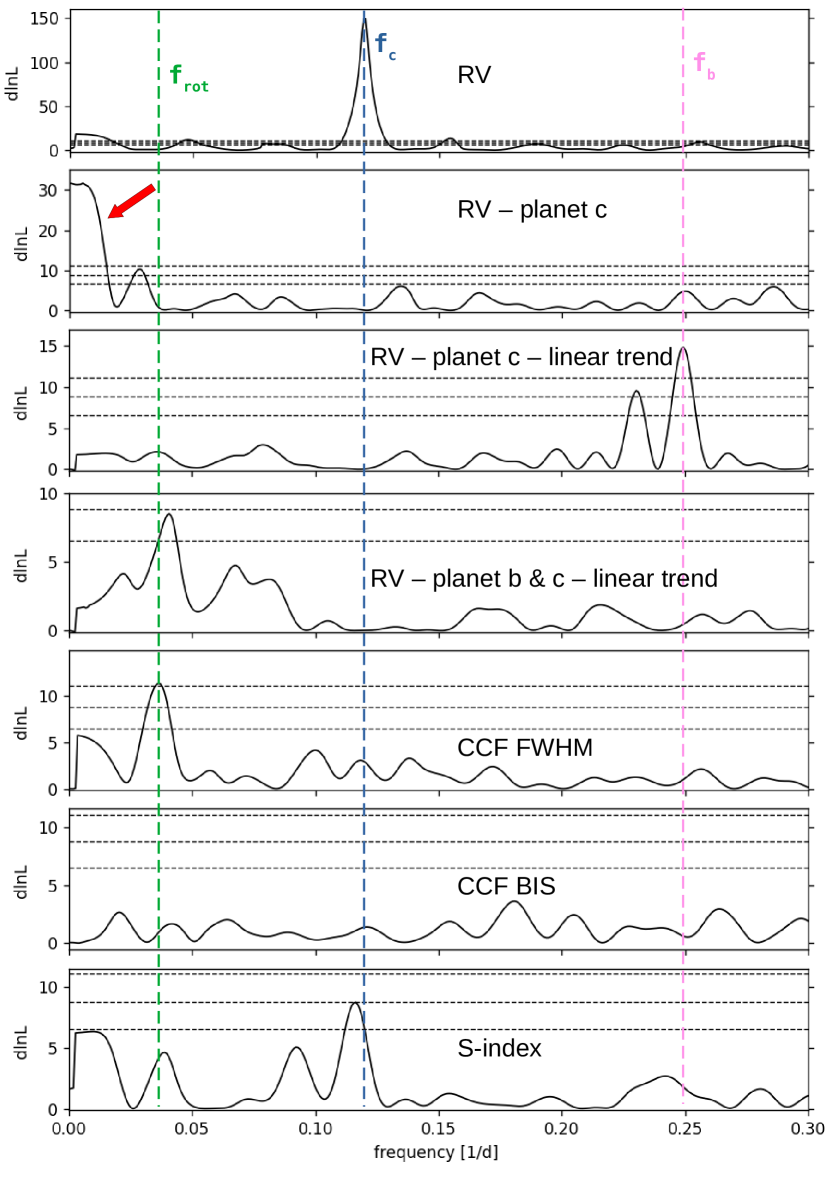
Figure 1: Maximum likelihood periodograms of the HARPS+PSF RV measurements and HARPS activity indicators. The blue and salmon vertical dashed lines mark the orbital frequencies of the two transiting planets, and the green vertical dashed line marks the rotation period of the star, while the horizontal dashed lines mark the 10 %, 1 % and 0.1 % false alarm probability. From top to bottom: RV data; RV residuals after subtracting the signal of TOI-1130 c; RV residuals after subtracting the signal of TOI-1130 c and a linear trend; RV residuals after subtracting the signals of TOI-1130 b & c and a linear trend; FWHM and BIS of the CCF; S-index. The red arrow in the third panel marks the excess of power at low frequencies significantly detected in the HARPS RVs.

The results of the maximum likelihood periodogram (MPL) as implemented in EXOSTRIKER (Trifonov 2019) are shown in Fig. 1. The HARPS and PFS RVs display a significant peak at the transit frequency of the outer giant planet TOI-1130 c ($f_{\mathrm{c}}$ $\approx$ 0.120 days^-1; Fig. 1, upper panel).We subtracted the Doppler signal induced by TOI-1130 c by fitting the RV time series, assuming that the planet has a circular Keplerian orbit. The MPL periodogram of the RV residuals (second panel in Fig. 1) shows a significant excess of power at frequencies lower than $\sim$ 0.014 days^-1, the spectral resolution of our RV data, indicating the presence of a long-term trend in our Doppler measurements (red arrow in Fig. 1, second panel). This peak has no counterpart in any of the periodograms of the activity indicators, suggesting that it could potentially be produced by an additional outer orbiting companion (see Sect. 4). After subtracting the previously detected signals, the residuals shown in the third panel of Fig. 1 show a significant peak at the transit frequency of the inner planet TOI-1130 b ($f_{\mathrm{b}}$ $\approx$ 0.245 days^-1). This peak is not significantly detected in any of the activity indicators, namely the CCF FWHM and BIS, and the S-index (Fig. 1, fifth, sixth, and seventh panel), spectroscopically confirming that the transit signal detected by TESS is due to planet b. The RV residuals following the subtraction of the Doppler motion induced by the two transiting planets and the linear trend (Fig. 1, fourth panel), display a peak at $\sim$ 0.041 days^-1 (i.e., $\sim$ 24.4 days) with a false alarm probability of FAP $\approx$ 1 %. Although the RV residuals’ peak is insignificant, we note that this peak and the peak in the CCF FWHM ($\sim$ 0.0.037 days^-1; Fig. 1, fifth panel) with a FAP of $\approx$ 0.1 % are virtually indistinguishable. Their difference of 0.004 days^-1 is 3.5 times smaller than the spectral resolution of our RV time-series (0.014 days^-1). Given the K6-K7 spectral type of TOI-1130 (Table 2), the signal at $\sim$ 27 days is very likely due to the presence of photospheric active regions carried around by stellar rotation. As such, we interpret the signal at $P_{\mathrm{rot}}$ $\approx$ 27 days as the star’s rotation period. The S-index shows a peak close to the orbital frequency of planet c, but with a FAP of 1 % it is not significant.

3.4 Photometric modeling

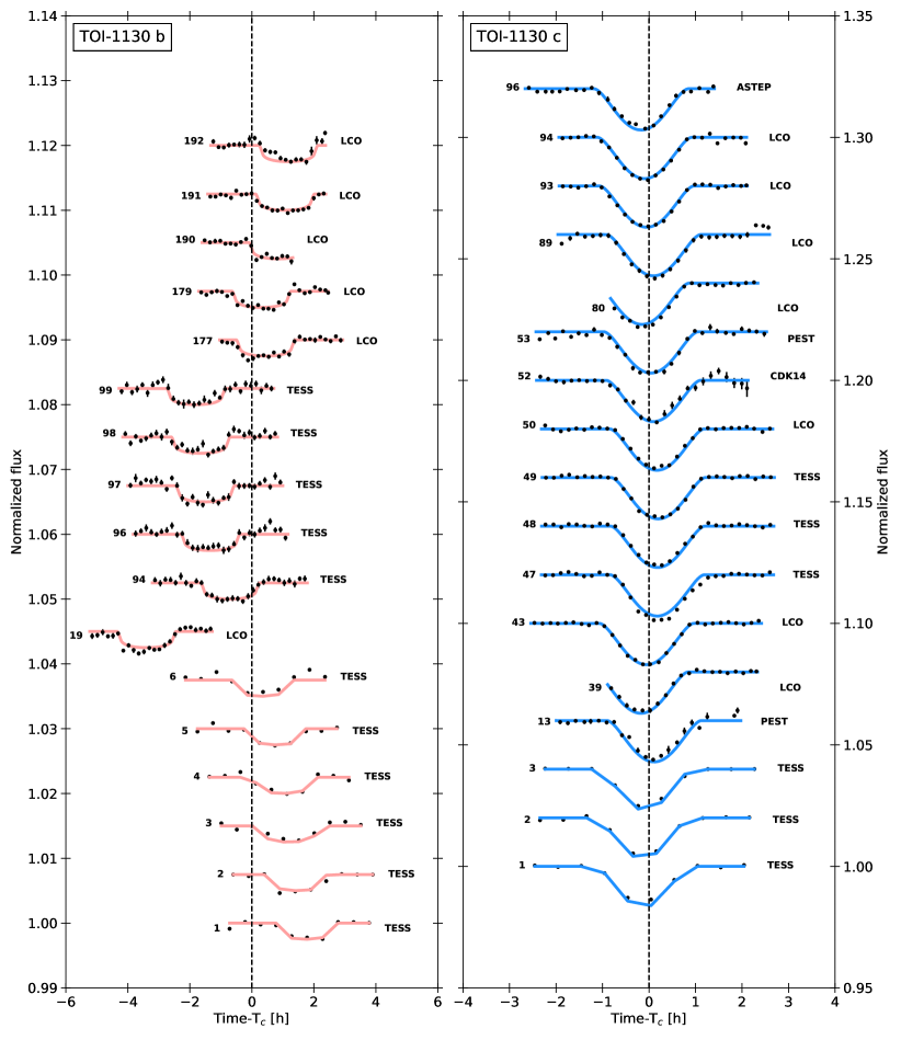
Figure 2: Detrended TESS and ground-based light curves for TOI-1130 b (left) and for TOI-1130 c (right). The light curves are shifted in phase according to the derived linear mean orbital period of each planet and shifted arbitrarily vertically for visibility. The corresponding transit number is shown on the left of each transit. For more details see Table 1. All light curves are binned to 10-min, except for the 30-min TESS light curves. The best-fit PyTTV transit model (see Sect. 3.4) is overplotted (TOI-1130 b: salmon and TOI-1130 c: blue). Note the different y-scales.

We fit the previously observed TESS and ground-based transits reported in Huang et al. (2020a) together with the new observations from TESS and the additional ground-based observations reported here using the Python Tool for Transit Variation (PyTTV; Korth 2020). This fit was done to first test whether the system shows TTVs and then to extract the transit center times for the photodynamical analysis. Other quantities were of no interest in this step.

PyTTV can search for and identify transit variations in light curves, and fit transits accounting for possible variations in the orbital period. By this method, the transits from both planets are modeled simultaneously using the quadratic Mandel & Agol (2002) transit model with the Taylor-series expansion from Parviainen & Korth (2020) as implemented in PyTransit (Parviainen 2015). For the 30-min cadence data from Sector 13, the transit model is super-sampled as suggested by Kipping (2010) to ensure a robust transit fit. The fit uses the orbital period $P$, the epoch $T_{0}$, the planet radius relative to stellar radius $R_{\mathrm{p}}/R_{\star}$ $\equiv$ $k$, the transit center times $T_{\mathrm{c}}$, and impact parameter $b$ for each planet as free parameters. Shared parameters during the fit are the quadratic limb darkening parameters $q_{1}$, $q_{2}$ as introduced in Kipping (2013), and the stellar density $\rho_{\star}$. We give each pass-band the same limb-darkening coefficients because limb darkening has little effect on the center time estimates. To account for stellar activity, we modeled the baseline as a Gaussian Process (GP) with a Matérn 3/2 kernel as implemented in celerite (Foreman-Mackey et al. 2017). We set wide normal priors on the orbital periods, the epochs, and the transit depths, where the prior means correspond to the values reported in ExoFOP-TESS. These priors are only weakly informative and do not constrain the posteriors in any significant way. They only aid the global optimizer. For the other parameters, we used uniform priors. We estimated the parameter posteriors using Markov Chain Monte Carlo (MCMC) sampling as implemented in emcee (Foreman-Mackey et al. 2013).

3.5 Photodynamical modeling

Table 3: Parameters of the TOI-1130 system. The values and the 1$\sigma$ uncertainties for planets in the TOI-1130 system are estimated through the photodynamical modeling using PyTTV. The reported osculating orbital elements are valid for the reference time $T_{0}$  = 2458657.

	TOI-1130
Fitted stellar parameters		Prior	Posterior
$R_{\star}$ [$R_{\odot}$ ]		$\mathcal{N}(0.68,0.02)$	0.695 $\pm$ 0.015
$M_{\star}$ [$M_{\odot}$ ]		$\mathcal{N}(0.71,0.02)$	0.712 $\pm$ 0.017
${q}_{1}$		$\mathcal{U}(0,1)$	0.65 $\pm$ 0.27
${q}_{2}$		$\mathcal{U}(0,1)$	0.31 $\pm$ 0.21
RV slope [m $\mathrm{s}^{-1}$ $\mathrm{days}^{-1}$]		$\mathcal{N}(0,1)$	0.495 $\pm$ 0.021
$\gamma_{\mathrm{HARPS}}$ [m $\mathrm{s}^{-1}$]		$\mathcal{N}(-7959,90)$	-7968.35 $\pm$ 0.37
$\gamma_{\mathrm{PFS}}$ [m $\mathrm{s}^{-1}$]		$\mathcal{N}(32,90)$	93.79 $\pm$ 0.78
RV-jitterHARPS[m $\mathrm{s}^{-1}$]		$\mathcal{N}(0,0.5)$	0.15 $\pm$ 0.16
RV-jitterPFS [m $\mathrm{s}^{-1}$]		$\mathcal{N}(0,0.5)$	0.37 $\pm$ 0.10
$P_{\mathrm{rot}}$ [days]		$\mathcal{N}(27,2)$	25.6 $\pm$ 1.2
Derived stellar parameters
$\rho_{\star}$ [g $\mathrm{cm}^{-3}$]		-	2.98 $\pm$ 0.18
	TOI-1130 b		TOI-1130 c
Fitted planet parameters	Prior	Posterior	Prior	Posterior
$P$ [days]	$\mathcal{N}(4.07,0.02)$	4.07445 $\pm$ 0.00046	$\mathcal{N}(8.35,0.02)$	8.350231 $\pm$ 0.000098
$T_{0}$ [BJD]	$\mathcal{N}(2458658.738,0.003)$	2458658.7405 $\pm$ 0.0013	$\mathcal{N}(2458657.798,0.003)$	2458657.90322 $\pm$ 0.00030
$\log_{10}$ $M_{\mathrm{p}}$ [$\log_{10}M_{\odot}$]	$\mathcal{U}(-5.5,-3.5)$	-4.237 $\pm$ 0.022	$\mathcal{U}(-4,-2)$	-3.0096 $\pm$ 0.0074
$R_{\mathrm{p}}/R_{\star}$	$\mathcal{U}(0.03,0.06)$	0.0470 $\pm$ 0.0011	$\mathcal{U}(0.09,0.25)$	0.175${}^{+0.018}_{-0.016}$
$\sqrt{e}\cos{\omega}$	$\mathcal{U}(-0.5,0.5)$	0.1358 $\pm$ 0.0021	$\mathcal{U}(-0.5,0.5)$	-0.010 $\pm$ 0.022
$\sqrt{e}\sin{\omega}$	$\mathcal{U}(-0.5,0.5)$	-0.1889 $\pm$ 0.0037	$\mathcal{U}(-0.5,0.5)$	-0.2124 $\pm$ 0.0040
$b$	$\mathcal{U}(-1,1)$	-0.518 $\pm$ 0.054	$\mathcal{U}(-1,1)$	-0.941${}^{+0.030}_{-0.032}$
$\Omega$ [rad]	$\pi$	$\pi$	$\mathcal{U}(0.5\pi,1.5\pi)$	3.1232 $\pm$ 0.0066
Derived parameters
$M_{\mathrm{p}}$ [$M_{\oplus}$ ]		19.28 $\pm$ 0.97		325.69 $\pm$ 5.59
$R_{\mathrm{p}}$ [$R_{\oplus}$ ]		3.56 $\pm$ 0.13		13.32${}^{+1.55}_{-1.41}$
$\rho_{\mathrm{p}}$ [g $\mathrm{cm}^{-3}$]		2.34 $\pm$ 0.26		0.75${}^{+0.31}_{-0.21}$
$e$	$\mathcal{N}(0,0.083)$	0.0541 $\pm$ 0.0015	$\mathcal{N}(0,0.083)$	0.0457 $\pm$ 0.0016
$\omega$ [∘]		144.24 $\pm$ 0.72		175.23 $\pm$ 4.24
$i$ [∘]		92.14 $\pm$ 0.26		92.44 $\pm$ 0.14
$a/R_{\star}$		13.77 $\pm$ 0.27		22.22 $\pm$ 0.44
$a$ [AU]		0.04457 $\pm$ 0.00036		0.07191 $\pm$ 0.00058
$T_{\mathrm{eq}}$ [K]		632.17 $\pm$ 12.60		497.70 $\pm$ 9.92
$F_{\mathrm{p}}$ [$F_{\oplus}$]		78.10 $\pm$ 5.55		30.00 $\pm$ 2.13

Since the planets strongly interact gravitationally with each other to produce significant TTVs as shown by the photometric modeling in the previous section (Fig. 2), we decided to model the RVs and the photometry simultaneously using a photodynamical model to determine the final planetary and orbital parameters. A photodynamical model combines a photometric transit model with N-body simulations whereby it produces a light curve that can be compared with observed light curves. The advantage of a photodynamical model is that it models the transit light curves taking into account the gravitational interaction between the bodies in the system. It models the transits simultaneously and includes also the transit shapes rather than only individual center times compared to traditional TTV analysis. This results in more robustly determined parameters as pointed out by several authors (e.g., Almenara et al. 2018). The disadvantage, however, is the high computational cost a photodynamical model needs. Here, we used the photodynamical model as implemented in PyTTV assuming a two-planet model, a sinusoidal RV signal to account for the stellar rotation, and a linear RV trend following the results from the periodogram analysis in Sect. 3.3. We briefly summarize the main parts of the photodynamical model.

The model uses the transit model with quadratic limb-darkening law described in Parviainen (2015) with the fast orbit computation introduced in Parviainen & Korth (2020), and the numerical N-body code Rebound with the IAS15 integrator (Rein & Liu 2012; Rein & Spiegel 2015) and the library Reboundx (Tamayo et al. 2020), to fit all the parameters without approximations. The transit model is super-sampled with ten samples per exposure for the long cadence observations (30-min), while short cadence observations (2-min) are calculated with one sample. We decided to fit the 2-min cadence instead of the 20-sec cadence because the 20-sec cadence would not lead to better time precision due to the relatively low S/N of the individual transits. The photodynamical model is parameterized by the stellar mass $M_{\star}$ and radius $R_{\star}$, the logarithms of the planet masses, planet radii relative to stellar radius $R_{\mathrm{p}}/R_{\star}$ $\equiv$ $k$, the impact parameters $b$, the quadratic limb darkening parameters $q_{1}$, $q_{2}$ defined in Kipping (2013), and the orbital elements (transit center time $T_{0}$, orbital period $P$, eccentricity $e$, argument of periastron $\omega$ where $e$ and $\omega$ are mapped from sampling parameters $\sqrt{e}\cos{\omega}$ and $\sqrt{e}\sin\omega$, longitude of the ascending node $\Omega$) at a reference time. The RV part adds further parameters, a linear trend, one offset for each telescope, three parameters for the sinusoidal function modeling the stellar activity (amplitude, period, and phase), and an RV-jitter term for each RV-data set.. The photometric variability is again modeled as a GP with a Matérn 3/2 kernel using celerite. The estimation of physical quantities is carried out via a global optimization followed by MCMC sampling using emcee to obtain samples from the posterior.

We fitted the TESS photometry from both sectors, the transit center times for the ground-based transits estimated in Sect. 3.4, and the RVs simultaneously with the photodynamical model. We decided to fit only for the ground-based transit center times rather than the full transits to simplify the process. We did not include the RV observed with CHIRON published in Huang et al. (2020a) since the RV uncertainties are 10 times larger for CHIRON than for HARPS or PFS (20 m $\mathrm{s}^{-1}$ vs. 2 m $\mathrm{s}^{-1}$). The photodynamical model was initialized with the values reported in Table 3 and has in total 28 free parameters: stellar mass and radius, six orbital elements, one mass and one radius ratio for each planet, two limb darkening coefficients, an RV trend, one RV offset for each telescope, amplitude, period and phase of the sinusoidal function, and two RV-jitter terms. We included an RV trend in the modeling to account for the Doppler signal induced by the potential outer companion detected in the HARPS data (Sect. 3.3). We decided to model this third signal as a trend given the relatively short baseline of our RV follow-up. The periodogram analysis (Sect. 3.3) also revealed the stellar rotational period. We thus decided to account for the stellar rotation signal in the RVs by including a sinusoidal function in the RV model. The period of the signal was loosely constrained by a normal prior (see Table 3), while its phase and amplitude were given non-constraining uniform priors.

The photodynamical modeling allows us to constrain the mutual inclination between the planets which is calculated via:

$$I=\cos^{-1}{(\cos{i_{\mathrm{b}}}\cos{i_{\mathrm{c}}}+\sin{i_{\mathrm{b}}}\sin{i_{\mathrm{c}}}\cos{(\Omega_{\mathrm{b}}-\Omega_{\mathrm{c}})})}.$$ (1)

Even if both planets were detected significantly in the RVs, we studied the effect of each observation method separately. Thus, we ran two additional photodynamical models where we used either only the RV measurements or the photometric observations to determine the system parameters.

4 Results

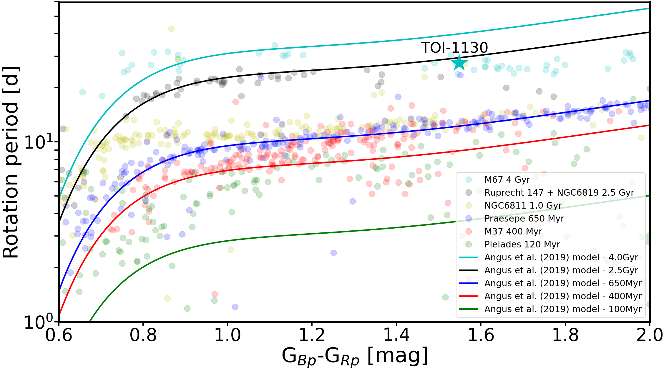
Figure 3: Gaia $B_{P}-R_{P}$ colour vs. rotation period diagram for TOI-1130 (cyan star) and members of well-studied clusters. Lines represent the empirical relation calibrated on the Praesepe cluster from Angus et al. (2019).

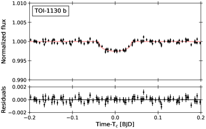
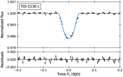
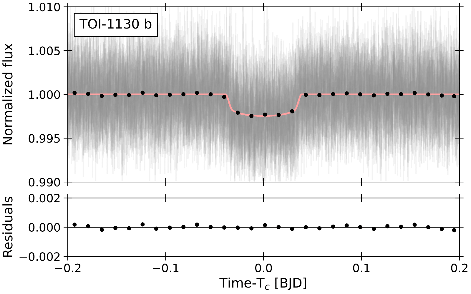
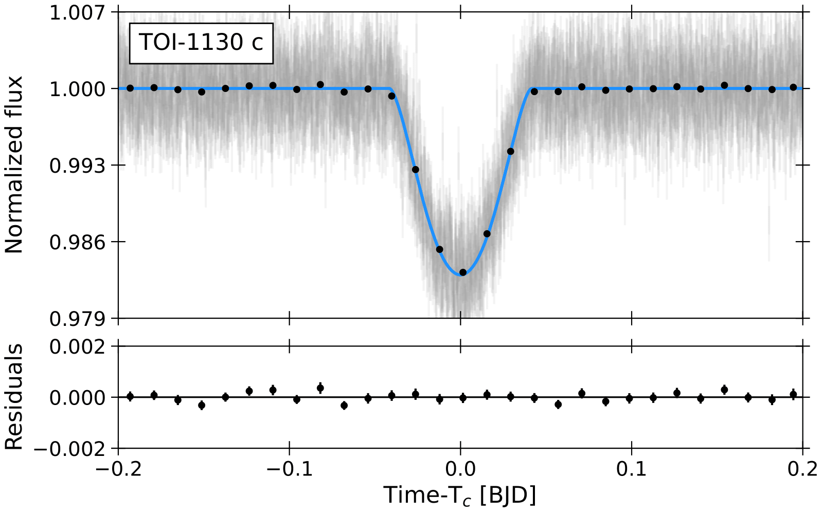
Figure 4: Phase-folded TESS transit light curves for TOI-1130 b (left) and for TOI 1130 c (right) accounting for the transit timing variations. The best-fit PyTTV transit model (see Sect. 3.4) is overplotted for both TOI-1130 b and TOI-1130 c color-coded in salmon and blue, respectively. The upper panels show the light curves from Sector 13 observed in the 30-min cadence mode (black points) and the lower panels show the light curves from Sector 27 observed in the 20-s cadence mode (grey points) with a binning of 20-min (black points). Residuals are shown beneath each plot.

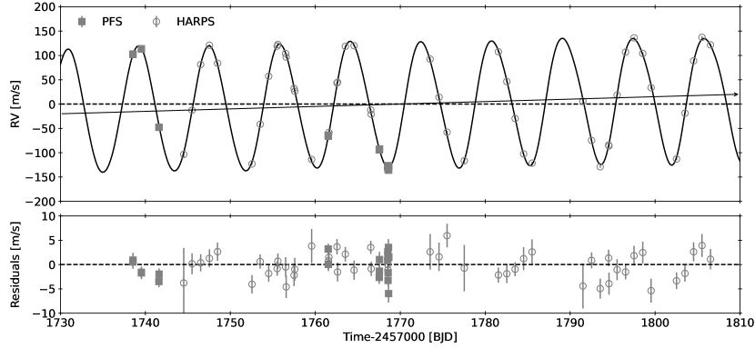
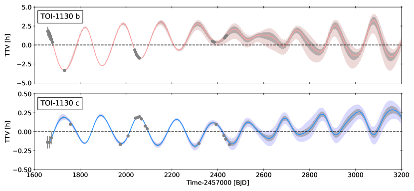
Figure 5: RV time series (upper panel) for TOI-1130 where the open circles and filled squares mark the data from HARPS and PFS, respectively. The best-fit PyTTV model (see Sect. 3.5) is overplotted in black. The data show a clear linear trend which is marked by the black arrow. RV residuals are shown in the second panel. Posterior TTV model (lower panels) from the photodynamical modeling of TOI-1130 b (third panel) and TOI-1130 c (fourth panel) with PyTTV (see Sect. 3.5). The solid salmon and blue colored lines mark the median of the posterior pdf while the shaded areas in grey and in light blue and pink show the 1 $\sigma$ and 3 $\sigma$ ranges for TOI-1130 b and TOI-1130 c, respectively. The TTVs with their individual uncertainties measured by fitting each transit center as an independent free parameter with PyTTV (Sect. 3.4) are shown in grey for comparison. The dashed lines mark the subtracted mean orbital period of 4.079$\pm$0.022 days with an ephemeris of 2458658.66924 $\pm$ 0.00020 days, and of 8.3495$\pm$0.0027 days with an ephemeris of 2458657.910329 $\pm$ 0.000046 days, respectively for TOI-1130 b and c.

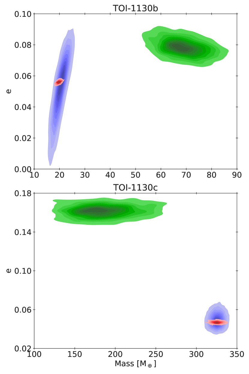
Figure 6: Eccentricity-mass-contour plot of the posteriors from the photodynamical model fitting RVs (blue) and TTVs (green) separately and simultaneously (red).

The values derived from iSpec and PARAM 1.5 agree with those inferred from VOSA and are adopted as the final stellar parameters.

We found that the light of TOI-1130 suffers a negligible reddening, as expected given the proximity of TOI-1130 to the Sun ($d=58.41\pm 0.07$ pc, Table 2). The V-band interstellar extinction $A_{\mathrm{v}}$ ranges between 0 and 0.05, depending on the atmospheric model used to fit the spectral energy distribution. As a reality check we modeled the SED following the method described in Gandolfi et al. (2008) and found an $A_{\mathrm{v}}$ = 0.03 $\pm$ 0.03, in agreement with the VOSA results.

The derived stellar parameters agree within 1$\sigma$ with the ones reported in Huang et al. (2020a) derived from SED fitting. Huang et al. (2020a) estimated a $v_{\mathrm{rot}}\sin{i_{\star}}$ = 4.0 $\pm$ 0.5 km $\mathrm{s}^{-1}$  from the light curve while our $v_{\mathrm{rot}}\sin{i_{\star}}$ $<$ 3 km $\mathrm{s}^{-1}$  estimated from iSpec is lower.

Our conservative stellar age determination of $4.86^{+3.38}_{-4.26}$ Gyr from stellar isochrones agrees within 1$\sigma$ with the lower end of the age $8.2^{+3.8}_{-4.9}$ Gyr derived by Huang et al. (2020a). Nevertheless, the age determination using isochrones of K dwarfs such as TOI-1130 is not reliable, since the star has already reached the main sequence. The periodogram analysis in Sect. 3.3 indicates a stellar rotational period of $\approx$ 27 days, which was confirmed in the photodynamical analysis to be 25.6 $\pm$ 1.2 days. To better constrain the system’s age, we compared the rotation period of TOI-1130 with the gyrochronology empirical relation from Angus et al. (2019) calibrated on the Praesepe cluster and the members of well-studied clusters studied in Godoy-Rivera et al. 2021: Pleiades cluster ($\sim$120 Myr), M37 cluster ($\sim$400 Myr), Praesepe cluster ($\sim$650 Myr), NGC 6811 cluster ($\sim$1 Gyr), together with the Ruprecht 147 + NGC 6819 clusters ($\sim$2.5 Gyr) studied in Curtis et al. 2020 and the M67 cluster ($\sim$4 Gyr) studied in Dungee et al. 2022. Each cluster was corrected for an interstellar extinction using the dustmaps code (Green 2018) and three-dimensional Bayestar dust maps (Green et al. 2019). We can see in Fig. 3 that the system’s age is consistent with the M67 cluster. Hence, we adopted the final age as an age of M67 from the literature. The age 3.2–5 Gyr is in agreement with the age derived by isochrones fitting.

We show the phase-folded transits from Sector 13 and 27 separately in Fig. 4 and the ground-based transits observed with the different facilities in Fig. 2 along with the phase-folded best-fit model from PyTTV (see Sect. 3.4). As seen from Fig. 2, both planets show significant TTVs as already suspected in Huang et al. (2020a). The newly observed TESS and ground-based transits confirm their expected TTV amplitude of at least two hours for planet b.

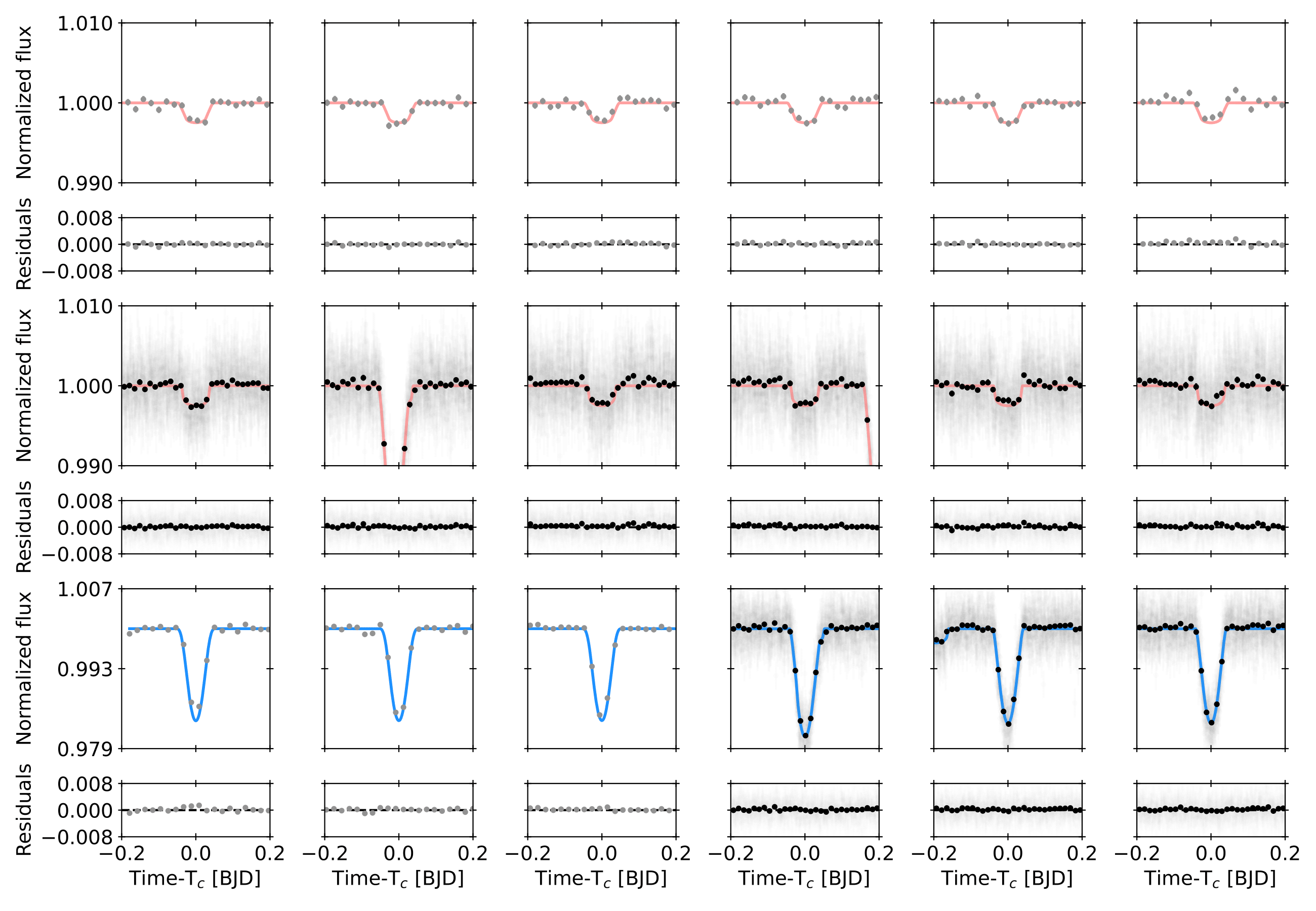
Figure 10: TESS transits of TOI-1130 b (upper two panels) and TOI-1130 c (lower panel) as used in the photodynamical modeling. Each transit is centred around the individual transit center times. The median PyTTV photodynamical model (see Sect. 3.5) is overplotted for both TOI-1130 b and TOI-1130 c color-coded in salmon and blue, respectively. The light curves from Sector 27 are binned to 20-min (black points). Residuals are shown beneath each plot.

The orbital and planetary parameters are derived from the photodynamical modeling that fits the RV, the TESS photometry, and the additional ground-based transit times simultaneously (Sect. 3.5) and reported in Table. 3. The RV model derived from the photodynamical fit to the HARPS and PFS RVs, the TESS photometry, as well as the ground-based transit center times, is shown in the upper panel of Fig. 5, while the TTV model is shown in the lower panels of Fig. 5. We show the individual photodynamical transit models to the TESS photometry in Fig. 10.

We show the eccentricity–mass contour plot of the photodynamical model fitting only the RVs, the TTVs, and the RVs and TTVs simultaneously in Fig. 6, to understand the contribution of both spectroscopic and photometric observations. The posterior using only the photometric data lies far from the posteriors fitting only the RVs and RV and TTV simultaneously. This difference is caused by insufficient coverage of the TTV phase. The planetary masses and orbital eccentricities cannot be derived from the current photometric data due to known mass-eccentricity degeneracy. The photometric solution fits a different posterior mode. Fitting only the RVs constrains the planetary masses tightly but leaves the eccentricity for the inner planet unconstrained. The photodynamical model that fits both the RVs and TTVs simultaneously allows us instead to put tight constraints on both the orbital eccentricities and planet masses of both planets.

The RV time series in the upper panel in Fig. 5 shows a significant linear trend (black arrow) likely due to the existence of an outer companion as uncovered by the frequency analysis (Sect. 3.3). To identify potential wide co-moving companion(s), we queried the Gaia  DR3 catalog through CDS/Vizier within a radius of one degree around TOI-1130. We used a radius of 1 mas and 5 mas in parallax and in each proper motion direction (right ascension and declination), respectively, to account for potential differences at large distances. This search did not return any companion. Following the procedure described in Smith et al. (2017), we constrained the properties of the outer planet $M_{\mathrm{d}}\,{a_{\mathrm{d}}}^{-2}\,=\,2.62\,M_{\mathrm{Jup}}\,\mathrm{AU}^{-2}$. If we assume a circular orbit for the outer companion and take our 70-day RV baseline, we find an orbital period of $\sim$ 140 days corresponding to a semi-major axis of $a_{\mathrm{d}}\,=\,0.47$ AU. This leads to a planet mass of $0.58$ $M_{\mathrm{Jup}}$. The maximal orbital distance assuming that the signal is planetary in nature ($M_{\mathrm{d}}\,=13$ $M_{\mathrm{Jup}}$) is 2.23 AU. The Gaia  DR3 release indicates a low RUWE of 1.137 and a null value for the non-single star table entry. However, TOI-1130 has a large sepsi parameter of 16.29, which indicates a significant excess in the astrometric noise (Lindegren et al. 2018). This excess might be related to the long linear trend seen in the RV time series.

The results derived here using the photodynamical model could change when considering a third planet in the system. However, since the third planet is to our best knowledge at the moment, further out, we expect no strong interactions with TOI-1130 b and TOI-1130 c and we can treat our result as valid. We find planetary masses for TOI-1130 b and TOI-1130 c of $M_{\mathrm{b}}\,=19.28\pm\,0.97$ $M_{\oplus}$ and $M_{\mathrm{c}}\,=325.69\pm\,5.59$ $M_{\oplus}$, and radii of $R_{\mathrm{b}}\,=3.56\pm\,0.13$ $R_{\oplus}$ and $R_{\mathrm{c}}\,=13.32^{+1.55}_{-1.41}$ $R_{\oplus}$, respectively. TOI-1130 c’s planetary mass and orbital parameters were previously determined by Huang et al. (2020a) based on RV measurements only. Our planetary mass and radius agree within 1 $\sigma$ with their values of $M_{\mathrm{c}}=309.56^{+13.67}_{-13.98}$ $M_{\oplus}$ and $R_{\mathrm{c}}=\leavevmode\nobreak\ 16.81^{+3.03}_{-2.47}$ $R_{\oplus}$. We reach a precision of 2% and 11% in planet mass and radius, which translates into a precision of 34%($\rho_{\mathrm{c}}\,=0.75^{+0.31}_{-0.21}\mathrm{cm}^{-3}$) in the mean density of TOI-1130 c. We refine the orbital eccentricity to $e_{\mathrm{c}}\,=\,0.0457\pm 0.0016$. TOI-1130 b was only validated in Huang et al. (2020a). We spectroscopically confirm the inner planet and measure its mass with a precision of 5%. We find that TOI-1130 b orbits the star on a slightly eccentric orbit with $e_{\mathrm{b}}\,=\,0.0541\pm 0.0015$. Our radius measurement of $R_{\mathrm{b}}\,=3.56\pm\,0.13$ $R_{\oplus}$ agrees within 1 $\sigma$ with $R_{\mathrm{b}}=3.65\pm 0.10$ $R_{\oplus}$ determined by Huang et al. (2020a). We reach a precision of 4% in the planet radius, which leads to a planetary density of $\rho_{\mathrm{b}}\,=\,2.34\pm\,0.26$ g $\mathrm{cm}^{-3}$ with a precision of 11%. We find a small mutual inclination of $\mathrm{I}=1.11\pm 0.39^{\circ}$ assuming $\Omega_{\mathrm{b}}=\pi$.

5 Discussion

We use the new system parameters derived in the previous sections to make inferences about the system’s dynamics and formations (Sect. 5.1), as well as the planet’s interiors (Sect. 5.2).

5.1 Dynamics and formation

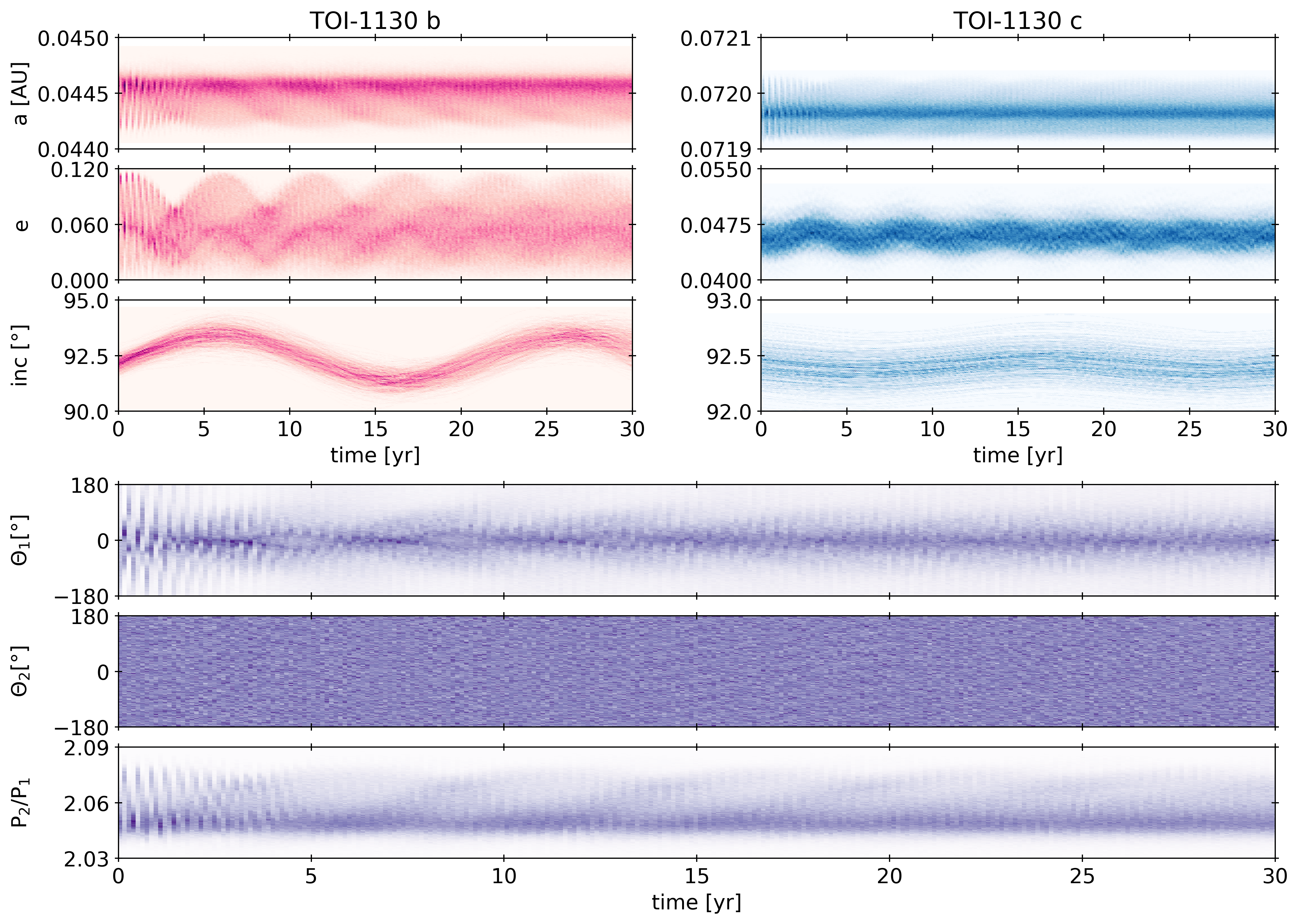
Figure 7: Evolution of TOI-1130’s orbital parameters reported in Table 3 for 30 years. Top panels: Evolution of the planetary semi-major axes, orbital eccentricities, and inclinations of TOI-1130 b (left) and TOI-1130 c (right). Lower panels: Evolution of the resonant angles $\Theta_{\mathrm{1}}$ and $\Theta_{\mathrm{2}}$, and the period ratio of TOI-1130 b and TOI-1130 c. The color shade represents the probability of the quantity having a certain value at a given time, with a darker shade indicating a higher probability. These probabilities were calculated based on the 600 dynamical simulations discussed in the text.

We performed a numerical stability analysis of the posterior from the photodynamical modeling to see if the planetary system lies in a stable configuration. The numerical simulations were carried out with the Rebound N-Body code with the IAS15 integrator. The system was simulated for $10^{7}$ years by drawing randomly 600 parameter combinations from the posterior in Table. 3. The posterior is found to lie in a stable configuration.

Since the system is close to a 2:1 period commensurability, we calculated the normalized distance to a $j:\leavevmode\nobreak\ j-1$ MMR as defined in Lithwick et al. (2012):

$$\Delta=\frac{P_{\mathrm{c}}}{P_{\mathrm{b}}}\frac{j-1}{j}-1,$$ (2)

where $P_{\mathrm{b}}$ and $P_{\mathrm{c}}$ are the orbital periods of the inner and outer planets. Using our 600 samples, we find $\Delta\,=\,0.02554\,\pm\,0.00009$, meaning that the two planets lie wide of their 2:1 resonance. To determine whether the planets are locked in resonance or not, we monitored the long-term evolution of the resonant angles during our stability simulation. For the 2:1 MMR, the resonant angles are defined as

$$\Theta_{\mathrm{1}}=2\lambda_{\mathrm{c}}-\lambda_{\mathrm{b}}-\varpi_{\mathrm{b}},$$ (3)

$$\Theta_{\mathrm{2}}=2\lambda_{\mathrm{c}}-\lambda_{\mathrm{b}}-\varpi_{\mathrm{c}},$$ (4)

where $\lambda_{\mathrm{i}}=M_{\mathrm{i}}+\varpi_{\mathrm{i}}$ is the mean longitude, $M_{\mathrm{i}}$ is the mean anomaly and $\varpi_{\mathrm{i}}=\omega_{\mathrm{i}}+\Omega_{\mathrm{i}}$ is the longitude of periapse (see Murray & Dermott 1999). Figure 7 shows the the results from the simulation: the evolution of the semi-major axis, eccentricities, inclinations, the resonant angles $\Theta_{\mathrm{1}}$ and $\Theta_{\mathrm{2}}$, and the orbital period ratio of TOI-1130 b and TOI-1130 c for 30 years. The resonant angle $\Theta_{\mathrm{1}}$ shows a libration around $0^{\circ}$ with a period of $4.5\,\pm\,0.3\,$years, while the amplitude is not constrained. The second resonant angle $\Theta_{\mathrm{2}}$ shows no libration and its amplitude is thus always $\pi$. Figure 8 shows the evolution of the trajectories of the resonant angles $\Theta_{1}$ and $\Theta_{2}$. There is a libration visible supporting that the system is in a 2:1 MMR. A study by Millholland et al. (2018) reports that the libration amplitudes of the resonant angles in the GJ 876 system seem to decrease with the amount of data used to characterize the system. Whether the libration amplitude of TOI-1130’s resonant angle will become detectable when more data are used or not, will be seen in the future when more data (RV and photometry) become available.

A planetary system in MMR needs either to be assembled during the gas phase of the disk when the planets can undergo convergent migration and find their stable resonant configuration while their eccentricities and inclinations are damped by the gas disk or via modest tidal migration (Delisle et al. 2014). In addition, a resonant system needs to survive the chaotic era after disk dispersal. Hence, multi-planet systems that are in MMR are well-preserved fossils from their formation era in the gas disk. Investigating their formation scenarios can provide clues to their natal disk properties (Hühn et al. 2021; Huang & Ormel 2022). The gravitational interaction between two planets in MMR can excite the planet’s eccentricity while gas disk-planet interaction damps them. The final eccentricities of planets’ are determined by which MMR the planets are in and how much damping from the disk is applied on the planets (e.g. Snellgrove et al. 2001; Lee & Peale 2002; Kley & Nelson 2012). Because the outer planet TOI-1130 c is much more massive than the inner one, it can give enough eccentricity to the inner planet to match our observations while it is difficult for TOI-1130 c to become eccentric unless an additional mechanism interferes. For example comparing Fig. 4, and 5 of Ataiee & Kley (2021) clearly shows that when the mass of the outer planet doubles in a two-planet system, the eccentricity of the inner planet considerably increases while the eccentricity of the outer planet remains similar to the equal-mass model. In addition, in their Fig. 10, they presented the results of a model identical to Fig 4 but with an additional third planet. In this model, the eccentricity of the second planet increased greatly compared to the two-planet model as the result of gravitational interaction with the third planet. However, for the case of massive planets in MMR, the eccentricity damping/excitation could be complicated and needs a more detailed study (e.g. Kley et al. 2005; Cimerman et al. 2018). Another mechanism suggested by Debras et al. 2021 needs the giant planet to be located at the appropriate position inside a disk inner cavity such that the Lindblad resonances which damp the planet’s eccentricity reside inside the cavity while those that excite the planet’s eccentricity lie in the disk, where the surface density is higher.

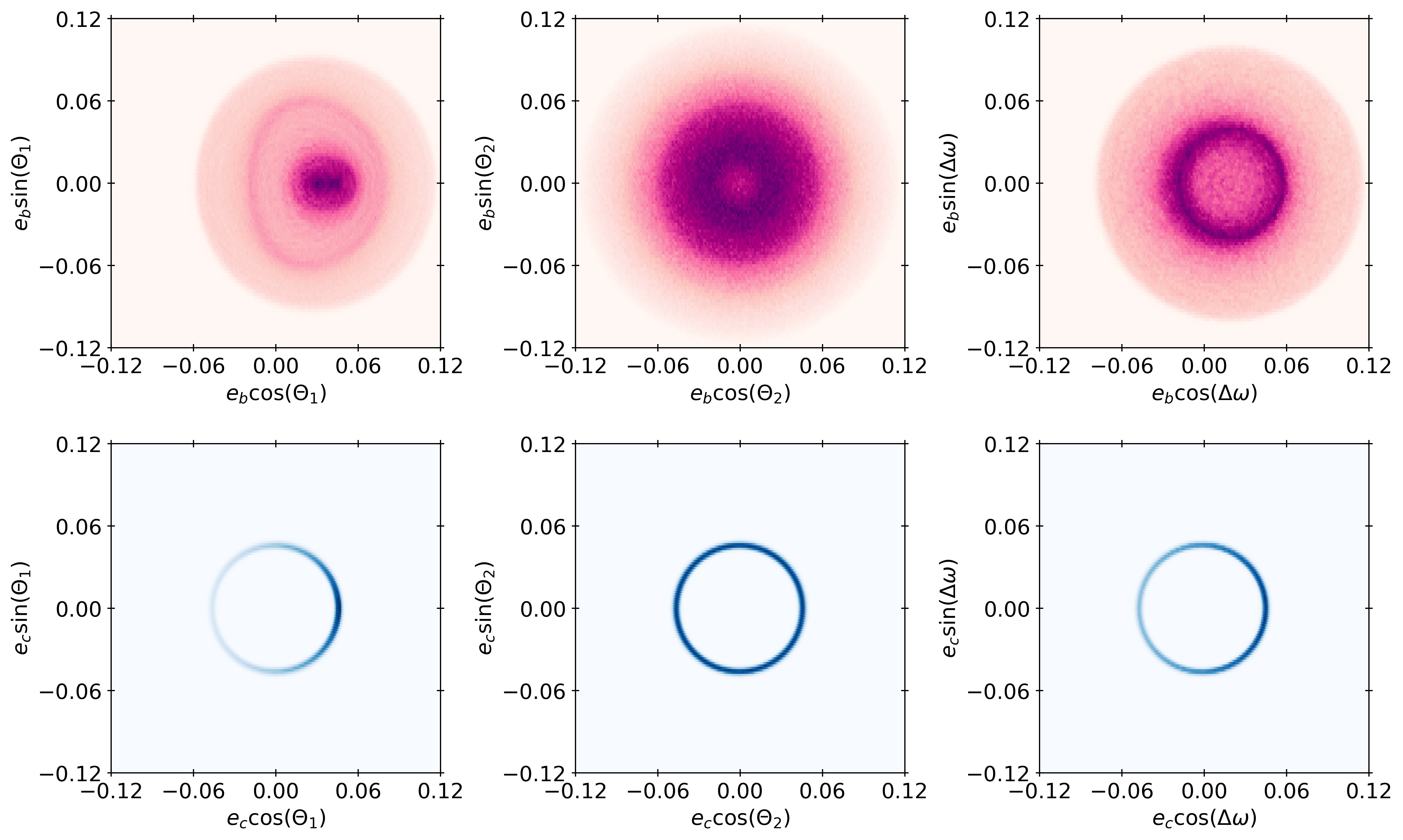
Figure 8: Evolution of the trajectories of the secular apsidal angle and resonant angles. The color shade is the same as in Fig. 7.

If the eccentricity of the hot Jupiter is a relic of formation, rather than ongoing planet–planet dynamics, it cannot have been damped by tidal interactions acting between the planet and the star over the system’s lifetime. For systems such as this, eccentricity decay is driven mainly by the tidal distortion of the planet by the star. We estimate the decay timescale for a constant-$Q$ tidal model using equation 1 of (Jackson et al. 2008):

$$\frac{\dot{e}}{e}=-\frac{63}{4}\left(GM_{\star}^{3}\right)^{1/2}\frac{R_{\mathrm{pl}}^{5}}{Q_{\mathrm{pl}}M_{\mathrm{pl}}}a^{-13/2},$$ (5)

where $Q_{\mathrm{pl}}$ is the tidal quality factor of the planet. We find a decay timescale of 5 Gyr occurs for a quality factor $Q_{\mathrm{pl}}\approx 5\times 10^{5}$; for comparison, our Solar System’s Jupiter has a quality factor around $10^{5}$ (Lainey et al. 2009) but a large spread of values is possible depending on the planet’s internal structure and the frequencies of the tidal forcing. It is therefore not possible to rule out a primordial origin of the eccentricity in this system, but tidal forces may well be significant in the long-term orbital dynamics.

5.2 Interior modeling

Knowing the radii and masses of several planets in the same system is extremely useful because one can remove the age uncertainty when comparing the planets to each other, thereby providing important constraints for formation models (Havel et al. 2011). Here we use CEPAM (Guillot & Morel 1995) and a non-grey atmosphere (Parmentier et al. 2015) to model the evolution of both planets in the system. We assume simple structures consisting of a central dense core and a surrounding hydrogen and helium envelope of solar composition. The core is assumed to be made with 50% of ices and 50% of rocks.

Figure 9 shows the resulting evolution models and observational constraints for both planets in the system. For guidance, we compare them to similarly simple models of Jupiter and Neptune (which have very similar masses as TOI-1130 c and TOI-1130 b, respectively), knowing that the ensemble of possibilities regarding their structure and composition is much wider (Helled & Fortney 2020). TOI-1130 c is found to have a small enrichment in heavy elements, with a core of less than 8 $M_{\oplus}$. This is lower to what was obtained for our simple model of Jupiter. We point out however that Jupiter’s enrichment corresponds to a much wider range of possibilities, i.e. 8 - 46 $M_{\oplus}$ (Guillot et al. 2022). TOI-1130 b is slightly more massive than Neptune but is found to contain less hydrogen and helium, assuming a similar composition core. With the same hypotheses, as shown in Fig. 9, the envelope of TOI-1130 b must be smaller than 0.5 $M_{\oplus}$ (i.e., less than 3% of the mass of TOI-1130 b compared to about 10% of the mass of Neptune).

Determining atmospheric abundances and possibly ice-to-rock ratios in TOI-1130 b and TOI-1130 c will be key to understanding the structure of ice and gas giants and the formation of these planetary systems (Guillot et al. 2022).

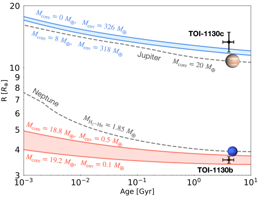
Figure 9: Evolution models of TOI-1130 b and TOI-1130 c compared to Neptune and Jupiter, respectively. All models assume a central ice-rock core overlain by a solar composition hydrogen-helium envelope. $M_{\rm core}$ corresponds to the mass of the core while $M_{\rm env}$ corresponds to the mass of the envelope. The range of envelope mass compatible with the observational constraints is shown for TOI-1130 b and compared to a similarly simple model of Neptune. For TOI-1130 c, only an upper limit on the core mass can be derived. For all cases, additional uncertainties on the core and envelope masses arise due to the unknown interior composition, temperature structure, and equation of state uncertainties. The black error bars correspond to observational constraints on the age and the radius of TOI-1130 b and TOI-1130 c.

6 Conclusions

We present a photodynamical analysis of the TOI-1130 planetary system that models consistently the TESS photometry, the HARPS and PFS RV measurements, and the ground-based photometry, accounting for the gravitational interaction between the bodies. The outer planet, TOI-1130 c, is a hot Jupiter that was previously detected and confirmed in Huang et al. (2020a), while the inner Neptune-sized planet, TOI-1130 b, was only validated. Here, both planets are confirmed and precisely characterized in terms of orbital parameters and planetary masses ($M_{\mathrm{b}}\,=19.28\pm\,0.97$ $M_{\oplus}$ and $M_{\mathrm{c}}\,=325.69\pm\,5.59$ $M_{\oplus}$) down to a precision of 5 % and 2 %, respectively. Due to the high impact parameter of the transit of TOI-1130 c, we can only determine its radius with a precision of 34 % ($R_{\mathrm{c}}\,=13.32^{+1.80}_{-1.21}$ $R_{\oplus}$) and its density with a precision of 35 % ($\rho_{\mathrm{c}}\,=0.75^{+0.31}_{-0.21}$ g $\mathrm{cm}^{-3}$). We find the radius of TOI-1130 b to be $R_{\mathrm{b}}\,=3.56\pm\,0.13$ $R_{\oplus}$ (4%), which translates into a precision of 11 % for its mean density ($\rho_{\mathrm{b}}\,=\,2.34\pm\,0.26$ g $\mathrm{cm}^{-3}$). The RV follow-up observations we carried out with the HARPS and PFS spectrographs unveiled a significant acceleration very likely induced by a massive outer companion.

Our mass estimates are mainly driven by the RVs and less by the photometry (Fig. 6). TOI-1130 should be monitored to allow for an independent mass measurement via photometry alone. TESS will re-observe TOI-1130 in Sector 67, until then further transit follow-up observations from the ground or from space, e.g., with the CHaracterising ExOPlanets Satellite (CHEOPS), are recommended to get an improved phase coverage of the TTVs. Furthermore, additional observations can confirm or reject the presence of the potential third planet.

TOI-1130 joins the small sub-sample of hot Jupiters with a nearby inner companion like WASP-47, Kepler-730, WASP-132, and TOI-2000. Our results show that TOI-1130 b and TOI-1130 c are most likely in 2:1 MMR which puts TOI-1130 in a unique position in this sample. Although it is not the first giant planet system found to be in a 2:1 resonant configuration, it is the first known system with a close-in gas giant and an inner low-mass planet locked in a 2:1 MMR. Other giant planet systems which are known to lie in such a resonant configuration consist of only warm giant planets ( e.g., HD 82943 (Tan et al. 2013), TOI-216 (Kipping et al. 2019: Dawson et al. 2019, 2021), TIC 279401253 (Bozhilov et al. 2023)). However, several giant planet systems with and without low-mass planets are known to lie near but not in a 2:1 resonance (e.g., Kepler-30 (Fabrycky et al. 2012; Panichi et al. 2018; Wu et al. 2018, Jontof-Hutter et al. 2022), Kepler-56 (Steffen et al. 2013; Huber et al. 2013; Otor et al. 2016), Kepler-88 (Nesvorný et al. 2013; Barros et al. 2014), Kepler-89 (Masuda et al. 2013; Weiss et al. 2013; Battley et al. 2021; Jontof-Hutter et al. 2022), TOI-2202 (Trifonov et al. 2021), TOI-2525 (Trifonov et al. 2023)).

Discoveries like TOI-1130 provide an important window into planetary formation. Such a system contradicts the formation pathway for hot Jupiters via HEM, which prohibits the formation of planets inside the orbit of the hot Jupiter. Formation via disk migration or in situ instead allows the existence of low-mass planets inside the orbit of a hot Jupiter. While planets that formed in situ show a wide range of period ratios, planets on near-resonant orbits seem to be more likely an outcome of disk migration or modest tidal migration. Therefore, it is more probable that this system is formed via migration than in situ. We note that even if the MMR favors the formation via disk migration, the observed low eccentricities are also consistent with the in situ formation. Therefore, further monitoring of this system is needed to distinguish between the two scenarios.

Atmospheric characterization of this system with the James Webb Space Telescope could help to distinguish between the formation models. Specifically, measuring the C/O abundances ratio could reveal whether the planets formed in situ or beyond the snow line (Öberg et al. 2011; Madhusudhan et al. 2014; 2017; Booth et al. 2017). We expect the planets to have different atmospheric compositions if they formed far away from each other, while the compositions should be similar if they formed close to each other. Furthermore, the C/O ratio gives us clues about where in the disk the planets have formed. However, measuring the C/O ratio is challenging since it requires precise measurements of C and O-bearing molecules which account for around 70% of the absorbers such as H₂O, CO, CO₂, and CH₄ and a good understanding of the underlying chemistry (Line et al. 2021; Fonte et al. 2023; Boucher et al. 2023).

Appendix A Radial velocities

Table 4: Radial velocity measurements and spectroscopic activity indicators for TOI-1130 from HARPS spectra

BJDTDB	RV	$\sigma$RV	BIS	FWHM	S-index	$\sigma$S-index	S/N	$t_{\mathrm{exp}}$
-2457000	[m $\mathrm{s}^{-1}$]	[m $\mathrm{s}^{-1}$]	[m $\mathrm{s}^{-1}$]	[m $\mathrm{s}^{-1}$]	-	-	@ 550 nm	[s]
1744.516586	-8071.84	7.19	53.17	6394.96	0.799	0.133	18.0	2100
1745.491812	-7981.02	2.15	51.91	6307.82	0.699	0.025	43.7	2100
1746.506986	-7887.07	1.76	52.82	6313.49	0.749	0.020	51.6	2100
1747.534521	-7847.40	1.84	50.74	6308.11	0.732	0.023	50.1	2100
1748.495349	-7884.41	1.86	47.21	6296.11	0.741	0.020	49.0	2100
1752.548748	-8091.47	1.88	49.45	6313.41	0.762	0.018	45.5	2100
1753.514551	-8009.94	1.46	46.58	6314.93	0.743	0.014	57.5	2100
1754.513913	-7911.19	1.69	53.57	6317.25	0.750	0.016	50.0	2100
1755.513265	-7849.18	1.45	53.29	6323.09	0.736	0.013	57.6	2100
1755.596208	-7845.92	1.55	43.68	6318.08	0.747	0.019	55.8	2100
1756.508322	-7864.35	2.02	49.33	6310.58	0.745	0.022	43.3	2100
1756.574080	-7871.85	2.31	41.50	6324.93	0.759	0.029	39.2	2100
1757.502187	-7936.45	2.22	44.92	6313.49	0.800	0.025	40.1	2100
1757.581857	-7941.94	2.35	51.72	6319.50	0.806	0.029	38.6	2100
1759.567931	-8082.26	3.49	54.33	6322.03	0.853	0.043	28.1	2100
1761.551634	-8032.14	1.77	36.48	6323.26	0.754	0.022	49.4	2100
1761.601212	-8026.75	1.73	47.81	6329.05	0.815	0.023	51.1	2100
1762.558170	-7924.98	1.56	49.49	6326.84	0.729	0.017	55.1	2100
1762.622204	-7923.65	1.94	45.11	6331.03	0.793	0.025	46.2	2100
1763.534758	-7849.78	1.50	52.98	6323.12	0.793	0.015	56.8	2100
1764.563457	-7848.33	1.96	46.44	6321.45	0.779	0.021	44.8	2100
1766.527451	-7980.54	1.35	55.60	6332.03	0.805	0.015	63.6	2100
1766.581646	-7989.46	1.47	53.24	6332.32	0.773	0.017	59.2	2100
1768.521916	-8098.51	1.44	48.83	6319.00	0.792	0.015	59.5	2100
1768.547573	-8099.68	1.50	47.68	6323.98	0.776	0.016	57.3	2100
1773.512029	-7875.94	3.65	34.78	6327.09	0.711	0.054	29.6	2100
1774.564408	-7954.29	2.92	57.44	6327.46	0.764	0.042	35.2	2100
1775.507737	-8026.29	2.43	44.21	6316.48	0.772	0.032	40.3	2100
1777.535606	-8084.98	4.77	60.32	6300.79	0.757	0.084	24.3	2100
1781.551841	-7860.85	1.54	49.56	6313.50	0.749	0.019	56.2	2100
1782.543742	-7922.02	1.91	50.68	6310.09	0.797	0.021	45.8	2100
1783.520045	-7998.14	1.44	50.81	6322.14	0.897	0.013	58.1	2100
1784.520593	-8070.87	2.35	54.33	6312.80	0.804	0.029	38.7	2100
1785.515228	-8089.91	2.58	45.32	6327.29	0.812	0.029	35.5	2100
1791.499671	-7962.54	4.61	76.81	6267.20	0.645	0.039	23.9	2100
1792.517829	-8043.12	1.63	54.64	6336.37	0.859	0.019	53.6	2100
1793.533452	-8097.38	2.04	61.37	6336.75	0.826	0.026	44.0	2100
1794.524991	-8052.72	1.69	55.51	6332.86	0.805	0.019	51.7	2100
1794.568008	-8054.37	2.26	48.31	6334.79	0.774	0.029	40.8	2100
1795.526473	-7949.96	2.15	46.31	6318.66	0.815	0.022	41.2	2100
1796.518281	-7861.47	1.52	49.39	6318.77	0.792	0.018	57.3	2100
1797.519454	-7832.17	2.03	54.43	6316.68	0.749	0.022	43.8	2100
1798.538403	-7864.31	2.22	54.98	6311.97	0.657	0.026	43.2	2100
1799.528154	-7934.69	2.44	48.59	6291.12	0.775	0.027	37.8	2100
1802.518128	-8081.30	1.68	41.05	6319.98	0.751	0.020	52.1	2100
1803.515728	-7987.21	1.69	54.63	6318.04	0.794	0.024	52.4	2100
1804.527948	-7879.48	1.96	48.16	6309.01	0.834	0.028	45.7	2100
1805.517277	-7831.15	2.36	45.07	6307.73	0.766	0.030	38.9	2100
1806.515287	-7846.64	2.09	40.90	6302.85	0.718	0.028	43.3	2100

Table 5: Radial velocity measurements and spectroscopic activity indicators for TOI-1130 from PFS spectra. 5% fractional uncertainty is assumed for the S-index and the H$\alpha$-index.

BJDTDB	RV	$\sigma$RV	S-index	$\sigma$S-index	H$\alpha$-index	$\sigma$H$\alpha$-index	$t_{\mathrm{exp}}$
-2457000	[m $\mathrm{s}^{-1}$]	[m $\mathrm{s}^{-1}$]	-	-	-	-	[s]
1738.530612	195.71	1.40	0.766	0.038	0.0478	0.0024	1200
1738.545340	196.86	1.51	0.870	0.043	0.0479	0.0024	1200
1739.523756	207.47	1.14	0.775	0.039	0.0475	0.0034	1200
1739.537905	206.97	1.27	0.824	0.041	0.0473	0.0024	1200
1741.595996	46.13	1.16	0.803	0.040	0.0470	0.0024	1200
1741.612304	46.22	1.16	0.778	0.039	0.0476	0.0024	1401
1761.520197	29.52	1.10	0.727	0.036	0.0476	0.0024	1200
1761.534865	27.71	1.37	0.804	0.040	0.0455	0.0023	1200
1767.524532	-0.34	1.33	0.829	0.041	0.0478	0.0024	1200
1767.539261	0.00	1.14	0.808	0.040	0.0475	0.0024	1200
1767.553969	1.45	1.57	0.898	0.045	0.0474	0.0024	1200
1768.520979	-35.39	1.43	0.856	0.043	0.0455	0.0023	1200
1768.534587	-33.59	1.06	0.839	0.042	0.0475	0.0024	1200
1768.549296	-34.44	1.16	0.846	0.042	0.0475	0.0024	1200
1768.563915	-39.56	1.15	0.808	0.040	0.0480	0.0024	1200
1768.577673	-38.01	1.40	0.869	0.043	0.0478	0.0024	1200
1768.608230	-32.8	1.71	0.903	0.045	0.0479	0.0024	1200
1768.623109	-42.27	1.84	0.873	0.044	0.0480	0.0024	1200
1768.638098	-34.79	1.88	0.907	0.045	0.0468	0.0023	1200
1768.652626	-34.61	1.65	0.876	0.044	0.0475	0.0024	1200

Appendix B Additional figures