Differentially Private Synthetic Data
via Foundation Model APIs 1: Images

Abstract

Generating differentially private (DP) synthetic data that closely resembles the original private data without leaking sensitive user information is a scalable way to mitigate privacy concerns in the current data-driven world. In contrast to current practices that train customized models for this task, we aim to generate DP Synthetic Data via APIs (DPSDA), where we treat foundation models as blackboxes and only utilize their inference APIs. Such API-based, training-free approaches are easier to deploy as exemplified by the recent surge in the number of API-based apps. These approaches can also leverage the power of large foundation models which are accessible via their inference APIs while the model weights are unreleased. However, this comes with greater challenges due to strictly more restrictive model access and the additional need to protect privacy from the API provider.

In this paper, we present a new framework called Private Evolution (PE) to solve this problem and show its initial promise on synthetic images. Surprisingly, PE can match or even outperform state-of-the-art (SOTA) methods without any model training. For example, on CIFAR10 (with ImageNet as the public data), we achieve FID$\leq$7.9 with privacy cost $\epsilon$ = $0.67$, significantly improving the previous SOTA from $\epsilon$ = $32$. We further demonstrate the promise of applying PE on large foundation models such as Stable Diffusion to tackle challenging private datasets with a small number of high-resolution images. The code and data will be released at https://github.com/microsoft/DPSDA.

1 Introduction

Figure 1: We consider the problem of generating DP synthetic data with API access to pre-trained models without any model training. This is in contrast to prior work which assumes full access to pre-trained models and requires training.

While data-driven approaches have been successful, privacy is a major concern. For example, statistical queries of a dataset may leak sensitive information about individual users [21]. Entire training samples can be reconstructed from deep learning models [29, 22, 8, 9, 10, 11, 12, 14, 53]. For example, [9] extracted some of the training images almost exactly from generations of Stable Diffusion model. Differential privacy (DP) is the gold standard in quantifying and mitigating these privacy concerns [20]. A DP algorithm ensures that information about individual samples in the original data cannot be inferred with high confidence from algorithm outputs. Differentially private synthetic data is the holy grail of DP research [35, 40, 6, 18, 54, 56, 32, 39, 24, 57, 31, 30, 48]. The goal is to generate a synthetic dataset that is statistically similar to the original data while ensuring DP. This has several benefits: (1) Thanks to the post-processing property of DP [21], we can use any existing non-private algorithm (such as training machine learning (ML) models) as-is on the synthetic data without incurring additional privacy loss. This is more scalable than redesigning and reimplementing every algorithm for DP. (2) Synthetic data can be shared freely with other parties without violating privacy. This is useful in situations when sharing data is necessary, such as when organizations (such as hospitals) want to release datasets to support open research initiatives [6, 40]. (3) Since synthetic data is DP, developers can look at the data directly which makes algorithm development and debugging a lot easier.

At the same time, with the recent advancement of powerful large foundation models, API-based solutions are gaining tremendous popularity, exemplified by the surge of GPT4-based applications. In contrast to the traditional paradigm that trains (or fine-tunes) customized ML models for each application, API-based solutions treat ML models as a blackbox and only utilize APIs that provide the input/output functions of the model. In fact, many foundation models including GPT4, Bard, and DALLE2 only provide API access without releasing model weights and code. Key reasons for the success of API-based solutions are that APIs offer a clean abstraction of ML and are readily available and scalable. Therefore, implementing and deploying these API-based algorithms is easier and faster even for developers without ML expertise. Such an approach can also leverage the power of foundation models that are only released through APIs. Unfortunately, the SOTA DP synthetic data algorithms today [24, 39] are still in the old paradigm: they need a customized training process for each dataset, whose implementation requires significant ML engineering efforts (§ 3).

Figure 2: Private Evolution (PE) framework for DP synthetic data. Left: Intuition of PE. Though private data and pre-trained generative models have very different distributions, the support of the former is likely to be covered by the support of the latter. We gradually shift the distribution of generated data toward private data through Private Evolution. Right: Algorithm of PE. We maintain a sample set (population), and iteratively select the most similar ones to the private samples (parents) and mutate them to generate the next population (offspring). The initial population and offspring are generated with foundation model APIs. Parent selection is done in DP using private samples.

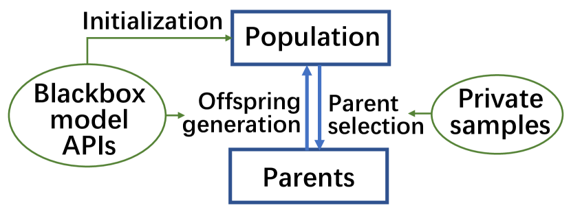
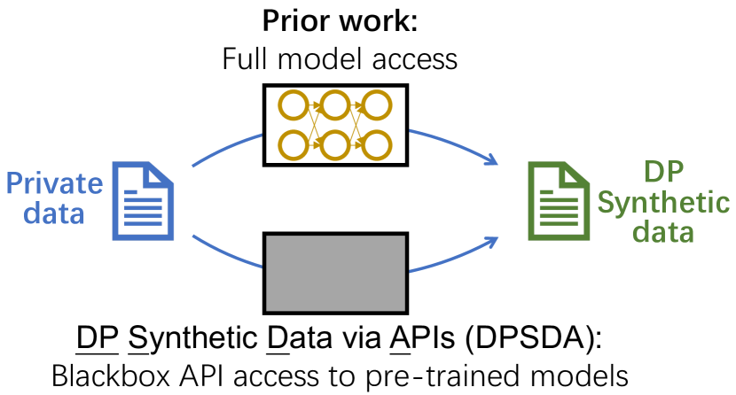
Motivated from these observations, we ask the following ambitious question (Fig. 1):

Can we generate DP synthetic data using blackbox APIs of foundation models?

Figure 3: Generated samples on CIFAR10 with $\left(0.67,10^{-5}\right)$-DP. Each row corresponds to one class. FID=7.87. See App. H for real and generated images side-by-side.

Figure 4: FID [33] (lower is better) v.s. privacy cost $\epsilon$ on CIFAR10 ($\delta=10^{-5}$). (Un)cond means (un)conditional generation. Ours achieves the best privacy-quality trade-off compared to DP-MEPF [31], DP-GAN, DP-Diffusion [24].

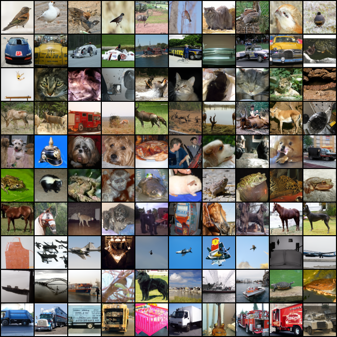
In our threat model, API providers are untrusted entities and we also want to protect user privacy from them, i.e., the API queries we make during generation should also be DP. If successful, we can potentially democratize the deployment of DP synthetic data in the industry similar to how API-based approaches have facilitated other applications. This is a challenging task, however, as we do not have access to model weights and gradients by assumption. In this paper, we conduct the first exploration of the potential and limits of this vision on DP synthetic images. Surprisingly, we show that not only is such a vision realizable, but that it also has the potential to match or improve SOTA training-based DP synthetic image algorithms despite more restrictive model access. Our contributions are:

(1) New problem (§ 3). We highlight the importance of DP Synthetic Data via APIs (DPSDA). Such algorithms are easy to implement and deploy and can leverage the foundation models behind APIs.

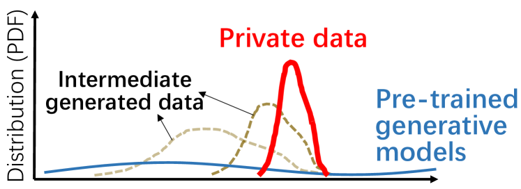
(2) New framework (§ 4). We propose an algorithm called Private Evolution (PE) for achieving our goal (Fig. 2). We consider using 2 popular APIs: random generation and sample variation (i.e., generating a sample similar to the given one).Footnotes 3 and 4 The key idea is to iteratively use private samples to vote for the most similar samples generated from the blackbox model and ask the blackbox models to generate more of those similar samples. We theoretically prove that the distribution of the generated samples from PE will converge to the private distribution under some modeling assumptions (§ 5). PE only requires (existing) APIs of the foundation models, and does not need any model training.

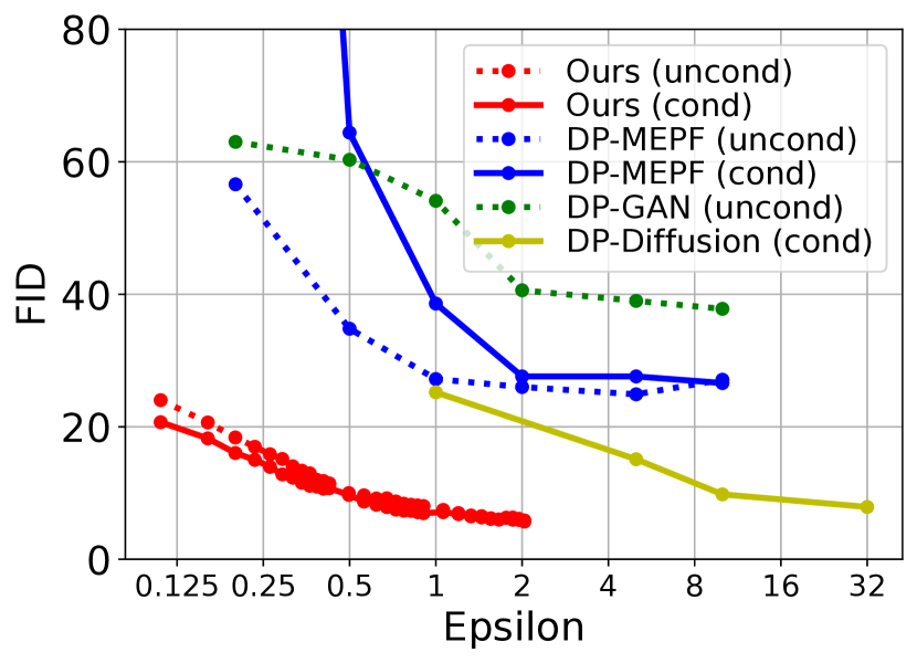
(3) Experimental results (§ 6). Some key results are: (a) Surprisingly, without any training, PE can still outperform SOTA training-based DP image generation approaches on some datasets (Figs. 4 and 4). For example, to obtain FID$\leq 7.9$ on CIFAR10 dataset, PE (with blackbox access to an ImageNet-pre-trained model) only needs $\epsilon=0.67$. In contrast, DP fine-tuning of an ImageNet-pre-trained model (prior SOTA) requires $\epsilon=32$ [24].
(b) We show that PE works even when there is significant distribution shift between private and public data. We create a DP synthetic version (with $\varepsilon=7.58$) of Camelyon17, a medical dataset for classification of breast cancer metastates (using the same ImageNet-pre-trained model). A downstream classifier trained on our DP synthetic data achieves a classification accuracy of 79.56% (prior SOTA based on DP fine-tuning is 91.1% with $\epsilon=10$ [24]).
(c) We set up new challenging benchmarks that the DP synthetic image literature has not studied before. We show that with powerful foundation models such as Stable Diffusion [47], PE can work with high-resolution (512x512) image datasets with a small size (100), which are common in practice but challenging for current DP synthetic image algorithms.

2 Background and Related Work

Differential Privacy (DP). We say a mechanism $\mathcal{M}$ is $(\epsilon,\delta)$-DP if for any two neighboring datasets $\mathcal{D}$ and $\mathcal{D}^{\prime}$ which differ in a single entry (i.e., $\mathcal{D}^{\prime}$ has one extra entry compared to $\mathcal{D}$ or vice versa) and for any set $S$ of outputs of $\mathcal{M}$, we have $\mathbb{P}\left(\mathcal{M}\left(\mathcal{D}\right)\in S\right)\leq e^{\epsilon}\mathbb{P}\left(\mathcal{M}\left(\mathcal{D}^{\prime}\right)\in S\right)+\delta$. Intuitively, this means that any single sample cannot influence the mechanism output too much.

DP synthetic data. Given a private dataset $\mathcal{D}$, the goal is to generate a DP synthetic dataset $\mathcal{M}\left(\mathcal{D}\right)$ which is statistically similar to $\mathcal{D}$. One method is to train a generative model from scratch on private data [40, 6, 18] with DP-SGD [1], a DP variant of stochastic gradient descent. Later studies show that pre-training generative models on public data before fine-tuning them on private data with DP-SGD [54, 56, 32, 39, 24, 57] gives better a privacy-utility trade-off due to knowledge transfer from public data [54, 23], smaller gradient spaces [38], or better initialization [23]. This approach achieves SOTA results on several data modalities such as text and images. In particular, DP-Diffusion [24] achieves SOTA results on DP synthetic images by pre-training diffusion models [49, 34, 43, 17] on public datasets and then fine-tuning the model on the private dataset. Some other methods do not depend on DP-SGD [35, 31, 30]. For example, DP-MEPF [31] trains generative models to produce synthetic data that matches the (privatized) statistics of the private features.

Note that all the above methods obtain generative models whose weights are DP, which can then be used to draw DP synthetic data. It is stronger than our goal which only requires DP synthetic data [41]. In this paper, we do not do any model training and only produce DP synthetic data.

3 DP Synthetic Data via APIs (DPSDA)

3.1 Motivation

As discussed in § 2, SOTA DP synthetic data algorithms require training or fine-tuning generative models with DP-SGD. There are some obstacles to deploying them in practice.

(1) Significant engineering effort. As discussed in § 1, deploying normal ML training pipelines is hard. Deploying DP training pipelines is even harder because most ML infrastructure is not built around this use case. Recently, there has been significant progress in making DP training more efficient [39, 32] and easy to use (Opacus [55] and Tensorflow Privacy). However, incorporating them in new codebases and new models is highly non-trivial. For example, to use Opacus, we need to implement our own per-sample gradient calculator for new layers. Common layers and loss functions that depend on multiple samples (e.g., batch normalization) are often not supported.

(2) Inapplicability of API-only models. It may be appealing to take advantage of the powerful foundation models in DP synthetic data generation. However, due to the high commercial value of foundation models, many companies choose to only release inference APIs of the models but not the weights or code. Examples include popular models such as DALLE 2 [46] and GPT 3/4 [7, 44] from OpenAI and Bard from Google. In such cases, existing training-based approaches are not applicable.

A DP synthetic data approach that only requires model inference APIs could potentially be deployed more easily. As the approach only depends on APIs, it does not need any modifications inside the model and requires minimal modifications when we switch to a different model (as long as they support the same APIs). Thus, it is easier to implement and use even for people without ML and DP expertise. In addition, such an approach is compatible with the models behind APIs.

3.2 Problem Formulation

We now give a formal statement of DPSDA. We first define a core primitive for DP synthetic data.

DP Wasserstein Approximation (DPWA). We are given a private dataset $S_{\mathrm{priv}}=\left\{x_{i}:i\in[N_{\mathrm{priv}}]\right\}$ with $N_{\mathrm{priv}}$ samples (e.g., images), a distance function $d(\cdot,\cdot)$ between samples and some $p\geq 1$. The goal is to design an $(\epsilon,\delta)$-DP algorithm $\mathcal{M}$ that outputs a synthetic dataset $S_{\mathrm{syn}}=\left\{x_{i}^{\prime}:i\in[N_{\mathrm{syn}}]\right\}$ with $N_{\mathrm{syn}}$ samples (as a multiset) whose distance to $S_{\mathrm{priv}}$, $W_{p}(S_{\mathrm{priv}},S_{\mathrm{syn}})$, is minimized. Here $W_{p}$ is the Wasserstein $p$-distance w.r.t. the distance function $d(\cdot,\cdot)$ (see App. A for the definition).

DPSDA. We want to solve DPWA where $\mathcal{M}$ is given blackbox access to foundation models trained on public data via APIs.Footnote 1 API queries should also be $(\epsilon,\delta)$-DP as API providers cannot be trusted.

In some applications, besides the raw samples $x_{i}$, we may also care about some auxiliary information such as class labels of images. In such cases, we may write $S_{\mathrm{priv}}=\left\{(x_{i},y_{i}):i\in[N_{\mathrm{priv}}]\right\}$ (and $S_{\mathrm{syn}}=\left\{(x_{i}^{\prime},y_{i}^{\prime}):i\in[N_{\mathrm{syn}}])\right\}$) where $y_{i}$ (and $y_{i}^{\prime}$) is the auxiliary information of $i$-th sample.

When the distance function $d(\cdot,\cdot)$ is $\ell_{2}$ (in the sample space), DPWA is closely related to DP Clustering [26, 51, 3] and DP Heatmaps [25]. But a direct application of these prior algorithms does not work in our setting; see App. F for more discussion on this.

3.3 Scope of This Work

Data type. While our framework above and our algorithms in § 4 are general for any data type, we focus on images in our experiments. We consider both unconditional (i.e., no $y_{i}$) and conditional generation tasks (e.g., $y_{i}$ can be image categories such as cats or dogs).

APIs. In our algorithm design and experiments, we use 2 APIs, both of which are either directly provided in the APIs of popular models (e.g., DALLE 2, Stable Diffusion) or can be easily implemented by adapting current APIs (e.g., using appropriate text prompts in GPT APIsFootnote 1):

(1) ${\textsf{RANDOM\_API}}{}\left(n\right)$ that randomly generates $n$ samples. Some APIs also accept condition information such as text prompts in text-to-image generation.Footnotes 3 and 4 For simplicity, we omit the condition information in the argument.

(2) ${\textsf{VARIATION\_API}}{}\left(S\right)$ that generates variations for each sample in $S$. For images, it means to generate similar images to the given one, e.g., with similar colors or objects.Footnotes 3 and 4 Some APIs also support setting the variation degree: ${\textsf{VARIATION\_API}}{}\left(S,v\right)$, where larger $v$ indicates more variation.

4 Private Evolution (PE)

Foundation models have a broad and general model of our world from their extensive training data. Therefore, we expect that foundation models can generate samples close to private data with non-negligible probability. The challenge is that by naively calling the APIs, the probability of drawing such samples is quite low. We need a way to guide the generation towards private samples.

Inspired by evolutionary algorithms (EA) [15] (App. B), we propose Private Evolution (PE) framework for generating DP synthetic data via APIs. See Fig. 2 for the intuition behind PE. The complete algorithm is in Alg. 1. Below, we discuss the components in detail.

Input :  Private samples: $S_{\mathrm{priv}}=\left\{x_{i}\right\}_{i=1}^{N_{\mathrm{priv}}}$

Number of iterations: $T$

Number of generated samples: $N_{\mathrm{syn}}$

Noise multiplier for DP Nearest Neighbors Histogram: $\sigma$

Threshold for DP Nearest Neighbors Histogram: $H$

Output :  Synthetic data: $S_{\mathrm{syn}}$

1 $S_{1}\leftarrow{\textsf{RANDOM\_API}}{}\left(N_{\mathrm{syn}}\right)$

2 for $t\leftarrow 1,\ldots,T$ do

       $histogram_{t}\leftarrow{\textsf{DP\_NN\_HISTOGRAM}}{}\left(S_{\mathrm{priv}},S_{t},\sigma,H\right)$

        // See Alg. 2

       $\mathcal{P}_{t}\leftarrow histogram_{t}/\mathrm{sum}(histogram_{t})$

        // $\mathcal{P}_{t}$ is a distribution on $S_{t}$

       $S_{t}^{\prime}\leftarrow$ draw $N_{\mathrm{syn}}$ samples with replacement from $\mathcal{P}_{t}$

        // $S_{t}^{\prime}$ is a multiset

3       $S_{t+1}\leftarrow{\textsf{VARIATION\_API}}{}\left(S_{t}^{\prime}\right)$

return $S_{T}$

Algorithm 1 Private Evolution (PE)

Input : Private samples: $S_{\mathrm{priv}}$

Generated samples: $S=\left\{z_{i}\right\}_{i=1}^{n}$

Noise multiplier: $\sigma$

Threshold: $H$

Distance function: $d{}\left(\cdot,\cdot\right)$

Output : DP nearest neighbors histogram on $S$

1 $histogram\leftarrow[0,\ldots,0]$

2 for $x_{\mathrm{priv}}\in S_{\mathrm{priv}}$ do

3       $i=\arg\min_{j\in\left[n\right]}d{}\left(x_{\mathrm{priv}},z_{j}\right)$

4       $histogram[i]\leftarrow histogram[i]+1$

$histogram\leftarrow histogram+\mathcal{N}\left(0,\sigma I_{n}\right)$

  // Add noise to ensure DP

$histogram\leftarrow\max\left(histogram-H,0\right)$

  // ‘max’, ‘-’ are operated element-wise

return $histogram$

Algorithm 2 DP Nearest Neighbors Histogram

Initial population (Alg. 1). We use RANDOM_API to generate the initial population. If there is public information about the private samples (e.g., they are dog images), we can use this information as prompts to the API to seed a better initialization.

Fitness function (Alg. 1 or Alg. 2). We need to evaluate how useful each sample in the population is for modeling the private distribution. Our idea is that, if a sample in the population is surrounded by many private samples, then we should give it a high score. To implement this, we define the fitness function of a sample $x$ as the number of private samples whose nearest neighbor in the population is $x$. A higher fitness value means that more private samples are closest to it. More details are below:

(1) Distance function (Alg. 2, Alg. 2). To define “nearest neighbor”, we need a distance function that measures the closeness or similarity of two samples. A naive way is to use $\ell_{2}$ distance $d{}\left(x,z\right)=\left\lVert x-z\right\rVert_{2}$, where $x$ is from the private dataset and $z$ is from the population. However, it is well-known that $\ell_{2}$ distance on pixel space is not a good metric for images. For example, a small shift of an object can result in a high $\ell_{2}$ distance. We therefore compute the $\ell_{2}$ distance in the embedding space:

$$d{}\left(x,z\right)=\left\lVert\Phi\left(x\right)-\Phi\left(z\right)\right\rVert_{2}$$ (1)

where $\Phi$ is a network for extracting image embeddings such as inception embedding [52] or CLIP embedding [45]. In general, which distance function to use will depend on the particular application and choosing the right one is critical for the algorithm to work well.

(2) Lookahead. The above approach gives high scores to the good samples in the current population. However, as we will see later, these good samples will be modified through VARIATION_API for the next population. Therefore, it is better to “look ahead” to compute the distance based on the modified samples as if they are kept in the population. We modify Eq. 1 to compute the distance between the embedding of $x$ and the mean embedding of $k$ variations of $z$: $d{}\left(x,z\right)=\left\lVert\Phi\left(x\right)-\frac{1}{k{}}\sum_{i=1}^{k}\Phi\left(z^{i}\right)\right\rVert_{2}$, where $k$ is called lookahead degree, and $z^{1},\dots,z^{k}$ are variations of $z$ obtained via VARIATION_API.

(3) Noise for DP (Alg. 2, Alg. 2)). Because this step utilizes private samples, we need to add noise to ensure DP. We add i.i.d. Gaussian noise from $\mathcal{N}\left(0,\sigma\right)$. The privacy analysis is presented in § 4.2.

(4) Thresholding (Alg. 2, Alg. 2)). When the number of generated samples is large, the majority of the histogram will be DP noise added above. To make the signal-noise ratio larger, we set a threshold $H$ to each bin of the histogram. Similar ideas have been used in DP set union [28].

In summary, we called the above fitness function DP Nearest Neighbors Histogram.

Parent selection (Alg. 1). We draw samples from the population according to the DP Nearest Neighbors Histogram so that a sample with more private samples around is more likely to be selected.

Offspring generation (Alg. 1). We use VARIATION_API to get variants of the parents as offsprings.

Conditional generation. The above procedure is for unconditional generation. To support conditional generation, i.e., each generated sample is associated with a label such as an image class (e.g., cats v.s. dogs), we take a simple approach: we repeat the above process for each class of samples in the private dataset. See Alg. 3 for the full algorithm.

4.1 Generating Unlimited Number of Samples

Our algorithm in Alg. 1 is preset with a fixed number of generated samples $N_{\mathrm{syn}}$. What if users want more samples afterward? In prior training-based methods [24], this is easy to achieve: one can draw an arbitrary number of samples from the trained generative models without additional privacy cost. In this section, we want to highlight that PE can also do that, again with API access only. We can simply generate unlimited number of samples by calling variation API with the generated dataset: ${\textsf{VARIATION\_API}}{}\left(S_{\mathrm{syn}}\right)$. In 6.1.3, we will see that this simple algorithm is sufficient to provide more useful samples for downstream applications.

4.2 Privacy Analysis

The only step that touches private data is Alg. 2. This can be regarded as a function $f$ whose input is the entire private dataset, and whose output is a histogram of votes with size $N_{\mathrm{syn}}$. Since each private sample only contributes 1 vote (Alg. 2), the $\ell_{2}$ sensitivity of $f$ when we add or remove a sample from $S_{\mathrm{priv}}$ is obviously 1. Based on this, Alg. 1 can be seen as $T$ (adaptive) compositions of Gaussian mechanism with noise multiplier $\sigma$ which is equivalent to a single Gaussian mechanism with noise multiplier $\sigma/\sqrt{T}$ [19]. We use the explicit formula for Gaussian mechanism [4] to compute the final privacy parameters. Here we consider the unconditional version of the algorithm; the privacy cost of the conditional version (Alg. 3) can be analyzed in the same way (App. C).

This privacy analysis implies that releasing all the (intermediate) generated sets $S_{1},S_{2},\dots,S_{T}$ also satisfies the same DP guarantees. Therefore PE provides the same privacy even from the API provider.

5 Theoretical Evidence for Convergence of PE

In this section, we will give some intuition for why PE can solve DPWA.

Convergence of Non-Private Evolution. We first analyze Alg. 1 when no noise is added to the histograms (i.e., we set $\sigma=0$ and $H=0$ in Alg. 1). We show that in this case, the evolution algorithm does converge to the private distribution in $O(d)$ iterations where $d$ is the dimension of the embedding space. Under some reasonable modeling assumptions (see App. D), we prove the following theorem. Here $D$ is the diameter of $S_{\mathrm{priv}}$, $L\approx$ number of variations of each point in $S_{t}^{\prime}$ that are added to $S_{t+1}$ in Alg. 1 of Alg. 1.

Theorem 1.

Assume that $\log L\ll d$. With probability $\geq 1-\tau$, the non-private evolution algorithm (Alg. 1 with $\sigma=H=0$) outputs $S_{\mathrm{syn}}$ with Wasserstein distance $W_{\infty}(S_{\mathrm{priv}},S_{\mathrm{syn}})\leq\eta$ after $T$ iterations whenever

$$T\gg\frac{d\log(D/\eta)}{\log L}+\log(N_{\mathrm{priv}}/\tau).$$ (2)

This theorem is nearly tight. In each iteration of PE, we get the voting information which is about $\tilde{O}(N_{\mathrm{priv}}\log(L))$ bits. To converge to $S_{\mathrm{priv}}$, we need at least $\tilde{\Omega}(N_{\mathrm{priv}}d)$ bits of information. Therefore we do require at least $\tilde{\Omega}(d/\log L)$ iterations to converge. Here is some intuition for how the proof of Thm. 1 works. Fix some private point $x\in S_{\mathrm{priv}}$. Let $z^{*}\in S_{t}$ be its closest point in $S_{t}$. In $S_{t+1}$, we generate variations of $z^{*}$ using the ${\textsf{VARIATION\_API}}{}\left(z^{*}\right)$. We then prove that if $\left\lVert x-z^{*}\right\rVert\geq\eta$, then one of the variations will get closer to $x$ than $z^{*}$ by a factor of $(1-(\log L)/d)$ with constant probability. Repeating this for $T$ iterations as in Eq. 2, will bring some point in $S_{T}$ $\eta$-close to $x$.

Convergence of Private Evolution. To get some intuition on the working of PE in the presence of noise, we make a simplifying assumption. We will assume that there are $B$ identical copies of each private point in $S_{\mathrm{priv}}$. We call $B$ as multiplicity. Note that for any DP algorithm to converge to $S_{\mathrm{priv}}$, we need that the private data is well clustered with some minimum cluster size. Any cluster with too few points cannot be represented in $S_{\mathrm{syn}}$, because that would violate DP. And when there is a cluster of $B$ private points and the generated points in $S_{t}$ are still far from this cluster, then it is likely that all the $B$ private points will have a common closest point in $S_{t}$, i.e., they all vote for the same point in $S_{t}$ as a single entity. Therefore multiplicity is a reasonable modeling assumption to make to understand the working of PE. Note that, actually it is very easy to find $S_{\mathrm{priv}}$ exactly using DP Set Union [28] with the multiplicity assumption. The point of Thm. 2 is to give intuition about why PE works in practice; it is proved in § D.2 under the same assumptions as in Thm. 1.

Theorem 2.

Let $0\leq\varepsilon\leq\log(1/2\delta)$. Suppose each point in $S_{\mathrm{priv}}$ has multiplicity $B$. Then, with high probability, Private Evolution (Alg. 1) with $\sigma\gg\sqrt{T\log(1/\delta)}/\varepsilon$ and $H=\sigma\sqrt{\log(TLN_{\mathrm{priv}})}$, when run for $T$ iterations, satisfies $(\varepsilon,\delta)$-DP and outputs $S_{\mathrm{syn}}$ such that $W_{\infty}(S_{\mathrm{priv}},S_{\mathrm{syn}})\leq\eta$ whenever $T$ satisfies Eq. 2 and $B\gg H\gg\frac{\sqrt{d\log(1/\delta)}}{\varepsilon}\mathrm{polylog}(dLN_{\mathrm{priv}}\log(D/\eta)/\tau).$

Thus, we should expect that PE will discover every cluster of private data of size $\gg\sqrt{d\log(1/\delta)}/\varepsilon$ in $O(d)$ iterations. We now compare this to previous work on DP clustering. [26] gives an algorithm for densest ball, where they show an $(\varepsilon,\delta)$-DP algorithm which (approximately) finds any ball of radius $r$ which has at least $\gg\sqrt{d\log(1/\delta)}/\varepsilon$ private points. Thus intuitively, we see that PE compares favorably to SOTA DP clustering algorithms (though we don’t have rigorous proof of this fact). If this can be formalized, then PE gives a very different algorithm for densest ball, which in turn can be used to solve DP clustering. Moreover PE is very amenable to parallel and distributed implementations. We therefore think this is an interesting theory problem for future work.

Why Private Evolution works well in practice. We have seen that in the worst case, PE takes $\Omega(d)$ iterations to converge. In our experiments with CIFAR10 and Camelyon17, where $d=2048$ is the embedding dimension, we see that PE actually converges in only about 20 iterations which is much smaller than $d$. We offer one plausible explanation for this via intrinsic dimension. Suppose the (embeddings of) realistic images lie on a low dimensional manifold $M$ inside $\mathbb{R}^{d}$ of dimension $d_{\mathrm{intrinsic}}\ll d$ (see experimental results in App. E). Given an image $z$, ${\textsf{VARIATION\_API}}{}\left(z\right)$ will create variations of $z$ which are also realistic images. Therefore the embeddings of these variations will also lie in the same manifold $M$, and PE is searching for the private points only inside the manifold $M$ without ever going outside it. Therefore the $d$ that matters for convergence is actually $d_{\mathrm{intrinsic}}\ll d.$ In this case, we expect that PE converges in $O(d_{\mathrm{intrinsic}})$ iterations and discovers clusters of private points of size at least $\sqrt{d_{\mathrm{intrinsic}}\log(1/\delta)}/\varepsilon$.

6 Experiments

In § 6.1, we compare PE with SOTA training-based methods on standard benchmarks to understand its promise and limitation. In § 6.2, we present proof-of-concept experiments to show how PE can utilize the power of large foundation models. We did (limited) hyper-parameter tunings in the above experiments; following prior DP synthetic data work [56, 24], we ignore the privacy cost of hyper-parameter tuning. However, as we will see in the ablation studies (§ 6.3 and K), PE stably outperforms SOTA across a wide range of hyper-parameters, and the results can be further improved with better hyper-parameters than what we used. Detailed hyper-parameter settings and more results such as generated samples and their nearest images in the private dataset are in Apps. H, I and J.

6.1 Comparisons to State-of-the-Art

Public information. We use standard benchmarks [24] which treat ImageNet [16] as public data. For fair comparisons, we only use ImageNet as public information in PE: (1) Pre-trained model. Unlike the SOTA [24] which trains customized diffusion models, we simply use public ImageNet pre-trained diffusion models (pure image models without text prompts) [43]. (2) Embedding (Eq. 1). We use ImageNet inception embedding [52]. PE is not sensitive to embedding choice though and we get good results even with CLIP embeddings (Fig. 32 in App. K).

Baselines. We compare with DP-Diffusion [24], DP-MEPF [31], and DP-GAN [31, 27]. DP-Diffusion [24] is the current SOTA that achieves the best results on these benchmarks.

Figure 5: Downstream classification accuracy (higher is better) on CIFAR10 ($\delta=10^{-5}$). The baseline results are taken from [24]. Two "ensemble" lines are from ensembles of 5 classifiers. The other two lines show the average accuracy of 5 independently trained classifiers with error bars. Our PE achieves better accuracy across almost all settings with smaller privacy costs.

Outline. We test PE on private datasets that are either similar to or differ a lot from ImageNet in § 6.1.1 and 6.1.2. We demonstrate that PE can generate an unlimited number of useful samples in § 6.1.3. We show that PE is computationally cheaper than train-based methods in App. L.

6.1.1 Moderate Distribution Shift (ImageNet $\rightarrow$ CIFAR10)

We treat CIFAR10 [37] as private data. Given that both ImageNet and CIFAR10 are natural images, it is a relatively easy task for PE (and also for the baselines). Figs. 4, 5 and 4 show the results. Surprisingly, despite the fact that we consider a strictly more restrictive model access and do not need training, PE can outperform the SOTA training-based methods. Details are below.

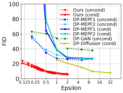
Sample quality v.s. privacy. Fig. 4 shows the trade-off between privacy cost and FID, a popular metric for image quality [33]. For either conditional or unconditional generation, PE outperforms the baselines significantly. For example, to reach FID$\leq 7.9$, [24] requires $\epsilon=32$, [31] cannot achieve it even with infinity $\epsilon$, whereas our PE only needs $\epsilon=0.67$.

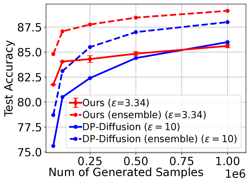
Downstream classification accuracy v.s. privacy. We train a downstream WRN-40-4 classifier [58] from scratch on 50000 generated samples and test the accuracy on CIFAR10 test set. This simulates how users would use synthetic data, and a higher accuracy means better utility. Fig. 5 shows the results (focus on the left-most points with num of generated samples = 50000 for now). [31] achieves 51% accuracy with $\epsilon=10$ (not shown). Compared with the SOTA [24], PE achieves better accuracy (+6.1%) with less privacy cost. Further with an ensemble of 5 classifiers trained on the same data, PE is able to reach an accuracy of 84.8%.

The above results suggest that when private and public images are similar, PE is a promising framework given its better privacy-utility trade-off and the API-only requirement.

6.1.2 Large Distribution Shift (ImageNet $\rightarrow$ Camelyon17)

Figure 6: Real and generated images from Camelyon17. More in App. I.

Next, we consider a hard task for PE, where the private dataset is very different from ImageNet. We use Camelyon17 dataset [5, 36] as private data which contains 302436 images of histological lymph node sections with labels on whether it has cancer (real images in Figs. 6 and 18). Despite the large distribution shift, training-based methods can update the model weights to adapt to the private distribution (given enough samples). However, PE can only draw samples from APIs as is.

We find that even in this challenging situation, PE can still achieve non-trivial results. Following [24], we train a WRN-40-4 classifier from scratch on 302436 generated samples and compute the test accuracy. We achieve 79.56% accuracy with $(7.58,3\cdot 10^{-6})$-DP. Prior SOTA [24] is 91.1% with $(10,3\cdot 10^{-6})$-DP. Random guess is 50%. Fig. 6 (more in Fig. 18) shows that generated images from PE are very different from ImageNet but similar to Camelyon17. Fig. 19 further shows how the generated images are gradually moved towards Camelyon17 across iterations.

These results demonstrate the effectiveness of PE. But when public models that are similar to private data are not available and when there is enough private data, the traditional training-based methods are still more promising at this point if the privacy-utility trade-off is the only goal. However, given the benefit of API-only assumption and the non-trivial results that PE already got, it is worth further exploiting the potential of PE in future work. Indeed, we expect these results can be improved with further refining PE (App. K).

6.1.3 Generating Unlimited Number of Samples

We use the approach in § 4.1 to generate more synthetic samples from § 6.1.1 and train classifiers on them. The results are in Fig. 5. Similar as [24], the classifier accuracy improves as more generated samples are used. With an ensemble of 5 classifiers, we reach 89.13% accuracy with 1M samples. This suggests that PE has the same capability as training-based methods in generating an unlimited number of useful samples. At the same time, we see that the gap between PE and DP-Diffusion diminishes as more samples are used. We hypothesize that it is due to the limited improvement space: As shown in [24], even using a ImageNet pre-trained classifier, the best accuracy DP-Diffusion achieves is close to the best points in Fig. 5.

6.2 More Challenging Benchmarks with Large Foundation Models

We demonstrate the feasibility of applying PE on large foundation models with Stable Diffusion [47].

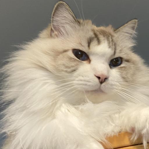
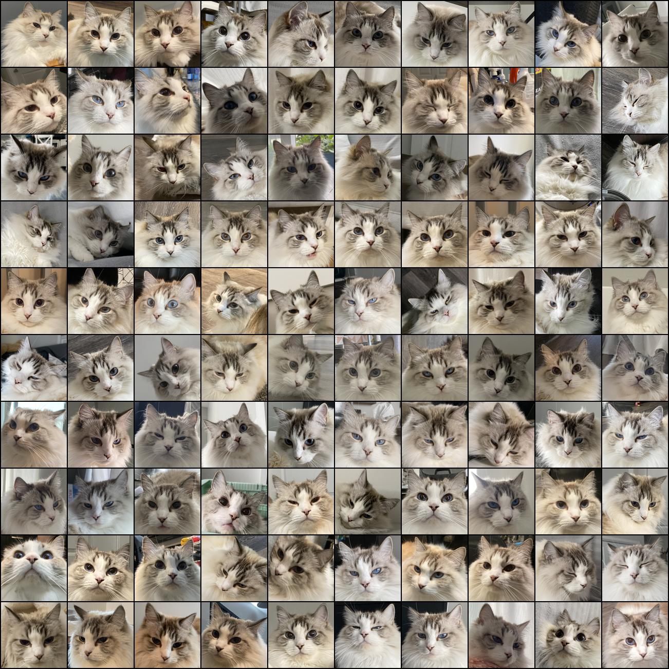
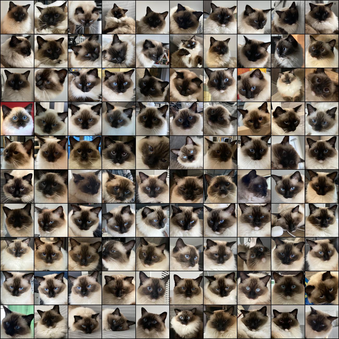
Data. Ideally we want to experiment with a dataset that has no overlap with Stable Diffusion’s training data. We take the safest approach: we construct two datasets with photos of the author’s two cats that have never been posted online. Each dataset has 100 512x512 images. Such high-resolution datasets with a small number of samples represent a common need in practice (e.g., in health care), but are challenging for DP synthetic data: to the best of our knowledge, no prior training-based methods have reported results on datasets with a similar resolution or number of samples. The dataset is released at https://github.com/microsoft/DPSDA as a new benchmark. See App. J for all images.

API implementation. We use off-the-shelf Stable Diffusion APIs (see App. J).

Results. We run Private Evolution for these two datasets with the same hyperparameters. Fig. 7 show examples of generated images for each of the cat datasets. We can see that Private Evolution correctly captures the key characteristics of these two cats. See App. J for all generated images.

Figure 7: Real and generated images from Cat Cookie (left) and Cat Doudou (right). More in App. J.

6.3 Ablation Studies

Pre-trained network. Fig. 8 shows the results with two different ImageNet pre-trained networks: one is larger (270M) with ImageNet class labels as input; the other one is smaller (100M) without label input (see App. G for implementation details). In all experiments in § 6.1, we used the 270M network. Two takeaways are: (1) The 270M network (trained on the same dataset) improves the results. This is expected as larger and more powerful models can learn public distributions better. This suggests the potential of PE with future foundation models with growing capabilities. (2) Even with a relatively weak model (100M), PE can still obtain good results that beat the baselines (though with a slower convergence speed), suggesting the effectiveness of PE.

More ablation studies are in App. K, where we see that PE obtains good results across a wide range of hyper-parameters, and the results shown before can be improved with better hyper-parameters.

Figure 8: Ablation studies on the pre-trained model. Both are public diffusion models trained on ImageNet [43]. The 270M network is conditional, whereas the 100M network is unconditional.

7 Discussion

Our work opens up new interesting research directions including:

Applications. (1) New privacy-preserving vision applications that were previously challenging but are now possible due to the new possibility of high-resolution DP synthetic images with small dataset sizes. (2) The use of PE in other data modalities beyond images such as texts.

Algorithms. (1) Minimizing number of API calls along with optimizing privacy vs utility tradeoff. (2) Leveraging the power of a large set of APIsFootnotes 3 and 4 beyond the two we used. (3) Algorithmic innovations to improve PE when the distributions of private data and foundation models are too different (§ 6.1.2). (4) Solving DPSDA in the Local/Shuffle DP model and in Federated Learning settings.

Appendix A Definition of Wasserstein Distance

Wasserstein distance is a widely used metric in designing [2] and evaluating [33] generative models. Given probability distributions $\mu,\nu$ on a metric space, the Wasserstein distance w.r.t. to a distance function $d(\cdot,\cdot)$ is defined as $W_{p}(\mu,\nu)=\inf_{\gamma}\left[\mathbb{E}_{(x,y)\sim\gamma}d(x,y)^{p}\right]^{1/p}$ where the infimum is over all couplings $\gamma$ of $\mu,\nu$. Also given discrete point sets $S,T$, we use $W_{p}(S,T)$ to denote the $W_{p}$-distance between uniform distributions on $S$ and $T$.

Appendix B A Brief Introduction to Evolutionary Algorithms

Evolutionary algorithms [15] are inspired by biological evolution, and the goal is to produce samples that maximize an objective value. It starts with an initial population (i.e., a set of samples), which is then iteratively updated. In each iteration, it selects parents (i.e., a subset of samples) from the population according to the fitness function which describes how useful they are in achieving better objective values. After that, it generates offsprings (i.e., new samples) by modifying the parents, hoping to get samples with better objective values, and puts them in the population. By doing so, the population will be guided towards better objective values.

We cannot directly apply existing EA algorithms to our problem. Firstly, our objective is to produce a set of samples that are jointly optimal (i.e., closer to the private distribution, § 3.2), instead of optimizing an objective calculated from individual samples in typical EA problems. In addition, the differential privacy requirement and the restrictive model API access are unique to our problem. These differences require us to redesign all components of EA.

Appendix C More Details on Private Evolution

Alg. 3 show the full algorithm that supports both unconditional data and conditional data. For simplicity, we assume that the private dataset $S_{\mathrm{priv}}$ is balanced, i.e., it has equal number of samples in each label class. Otherwise, we can first estimate the counts using the Laplace mechanism and use these counts to generate a synthetic data of appropriate size in each label class.

Input : The set of private classes: $C$     ($C=\left\{0\right\}$ if for unconditional generation)

Private samples: $S_{\mathrm{priv}}=\left\{(x_{i},y_{i})\right\}_{i=1}^{N_{\mathrm{priv}}}$, where $x_{i}$ is a sample and $y_{i}\in C$ is its label

Number of iterations: $T$

Number of generated samples: $N_{\mathrm{syn}}$   (assuming $N_{\mathrm{syn}}~{}\textrm{mod}~{}\left|C\right|=0$)

Noise multiplier for DP Nearest Neighbors Histogram: $\sigma$

Threshold for DP Nearest Neighbors Histogram: $H$

1 $S_{\mathrm{syn}}\leftarrow\emptyset$

2 for $c\in C$ do

3       $private\_samples\leftarrow\left\{x_{i}|(x_{i},y_{i})\in S_{\mathrm{priv}}\text{ and }y_{i}=c\right\}$

4       $S_{1}\leftarrow{\textsf{RANDOM\_API}}{}\left(N_{\mathrm{syn}}/\left|C\right|\right)$

5       for $t\leftarrow 1,\ldots,T$ do

             $histogram_{t}\leftarrow{\textsf{DP\_NN\_HISTOGRAM}}{}\left(private\_samples,S_{t},\sigma,H\right)$

              // See Alg. 2

             $\mathcal{P}_{t}\leftarrow histogram_{t}/\mathrm{sum}(histogram_{t})$

              // $\mathcal{P}_{t}$ is a distribution on $S_{t}$

             $S_{t}^{\prime}\leftarrow$ draw $N_{\mathrm{syn}}/|C|$ samples with replacement from $\mathcal{P}_{t}$

              // $S_{t}^{\prime}$ is a multiset

6             $S_{t+1}\leftarrow{\textsf{VARIATION\_API}}{}\left(S_{t}^{\prime}\right)$

7      $S_{\mathrm{syn}}\leftarrow S_{\mathrm{syn}}\cup\left\{(x,c)|x\in S_{T}\right\}$

return $S_{\mathrm{syn}}$

Algorithm 3 Private Evolution (PE) for both labeled and unlabeled data.

Privacy analysis. Following prior DP synthetic data work, we assume that the set of private classes $C$ (e.g., $\{$cats, dogs$\}$) is public information (but label assignments of samples are private). The privacy cost of Alg. 3 is the same as Alg. 1 shown in § 4.2. To see this, instead of looking at one call of Alg. 2, we consider $\left|C\right|$ calls of Alg. 2 at $t=t_{0}$ for all $c\in C$ as one “pseudo” function $f$. Same as the analysis in § 4.2, the input to this function is the entire private dataset, and the output is a histogram with size $N_{\mathrm{syn}}$. Therefore, the analysis in § 4.2 applies here.

Appendix D Proofs of PE Convergence Theorems

We will slightly modify the algorithm as necessary to make it convenient for our analysis. We will make the following modeling assumptions:

• The private dataset $S_{\mathrm{priv}}$ is contained in an $\ell_{2}$ ball of diameter $D$ and RANDOM_API will also produce initial samples in the same ball of diameter $D$.

• The distance function used in Alg. 2 is just the $\ell_{2}$ norm, $d(x,z)=\left\lVert x-z\right\rVert_{2}$.

• The distribution of points we output is $S_{\mathrm{syn}}=\mathcal{P}_{T}$ (i.e., we output a distribution of points).

• $S_{t}^{\prime}\supset\mathrm{supp}(\mathcal{P}_{t})=\mathrm{supp}(histogram_{t})$.

• $S_{t+1}=S_{t}^{\prime}\cup\bigcup_{z\in S_{t}^{\prime}}{\textsf{VARIATION\_API}}{}\left(z\right)$ where ${\textsf{VARIATION\_API}}{}\left(z\right)$ samples $L$ samples each from Gaussian distributions $\mathcal{N}(z,\sigma_{i}^{2}I)$ for $\sigma_{i}=\frac{D\sqrt{\log L}}{2^{i}d}$ where $1\leq i\leq r$ and $r=\log(D/\eta)$ where $\eta>0$ is the final Wasserstein distance.

D.1 Proof of Thm. 1

Proof.

Fix a point $x\in S_{\mathrm{priv}}$ and some iteration $t$. Suppose $z^{*}\in S_{t}$ is the closest point to $x$. Since $x$ will vote for $z^{*}$ in $histogram_{t}$, $z^{*}\in\mathrm{supp}(\mathcal{P}_{t})\subset S_{t}^{\prime}$. Therefore ${\textsf{VARIATION\_API}}{}\left(z^{*}\right)\subset S_{t+1}$. Let $V={\textsf{VARIATION\_API}}{}\left(z^{*}\right)$.

Claim 1.

If $\left\lVert x-z^{*}\right\rVert\geq\eta$, then with probability at least $1/2$, some point in $V$ will get noticeably closer to $x$ than $z^{*}$, i.e.,

$$\min_{z\in V}\left\lVert x-z\right\rVert_{2}\leq\left(1-\frac{\log L}{2d}\right)\left\lVert x-z^{*}\right\rVert_{2}.$$

Proof.

Let $s=\left\lVert x-z^{*}\right\rVert$ and let $\sigma\in\{\sigma_{1},\sigma_{2},\dots,\sigma_{r}\}$ be such that $\sigma d/\sqrt{\log L}\in[s/2,s]$. Note that such a $\sigma$ exists since $s\in[\eta,D]$. We will now prove that one of the $L$ samples $z_{1},z_{2},\dots,z_{L}\sim\mathcal{N}(z,\sigma^{2}I_{d})$ will get noticeably closer to $x$ than $z^{*}.$ Let $z_{i}=z^{*}+\sigma w_{i}$ where $w_{i}\sim\mathcal{N}(0,I_{d}).$

$$\min_{i\in[L]}\left\lVert x-z_{i}\right\rVert_{2}^{2} =\left\lVert x-z^{*}\right\rVert_{2}^{2}+\min_{i\in[L]}\left(\sigma^{2}\left\lVert w_{i}\right\rVert_{2}^{2}-2\sigma\left\langle x-z^{*},w_{i}\right\rangle\right)$$

$$\leq s^{2}+\max_{i\in[L]}\sigma^{2}\left\lVert w_{i}\right\rVert_{2}^{2}-\max_{i\in[L]}2\sigma\left\langle x-z^{*},w_{i}\right\rangle$$

Note that $\left\lVert w_{i}\right\rVert_{2}^{2}$ is a $\chi_{d}^{2}$ random variable. By using upper tail bounds for $\chi_{d}^{2}$ distribution and union bound over $i\in[L]$, we can bound

$$\Pr\left[\max_{i\in[L]}\left\lVert w_{i}\right\rVert_{2}^{2}\geq 3d/2\right]\leq L\exp(-\Omega(d))\ll 1.$$

The distribution of $\left\langle x-z^{*},w_{i}\right\rangle$ is the same as $\left\lVert x-z^{*}\right\rVert_{2}\tilde{w}_{i}$ where $\tilde{w}_{1},\dots,\tilde{w}_{L}$ are iid $N(0,1)$ random variables. By using the fact that max of $L$ iid Gaussians is at least $\sqrt{\log L}$ with probability at least $3/4$ (for $L\gg 1$), we get that

$$\Pr\left[\max_{i\in[L]}\left\langle x-z^{*},w_{i}\right\rangle\leq 2s\sigma\sqrt{\log L}\right]\leq\frac{1}{4}.$$

Combining everything we get:

$$\frac{1}{2} \geq\Pr\left[\min_{i\in[L]}\left\lVert x-z_{i}\right\rVert_{2}^{2}\geq s^{2}+(3/2)d\sigma^{2}-2s\sigma\sqrt{\log L}\right]$$

$$\geq\Pr\left[\min_{i\in[L]}\left\lVert x-z_{i}\right\rVert_{2}^{2}\geq\max_{\lambda\in[1/2,1]}s^{2}+(3/2)d\left(\frac{\lambda s\sqrt{\log L}}{d}\right)^{2}-2s\left(\frac{\lambda s\sqrt{\log L}}{d}\right)\sqrt{\log L}\right]$$

$$\geq\Pr\left[\min_{i\in[L]}\left\lVert x-z_{i}\right\rVert_{2}^{2}\geq s^{2}+\left(\frac{s^{2}\log L}{d}\right)\max_{\lambda\in[1/2,1]}(3\lambda^{2}/2-2\lambda)\right]$$

$$\geq\Pr\left[\min_{i\in[L]}\left\lVert x-z_{i}\right\rVert_{2}^{2}\geq s^{2}\left(1-\frac{\log L}{2d}\right)\right]$$

∎

Now in $T$ iterations, $\min_{z\in S_{t}}\left\lVert x-z\right\rVert_{2}$ will shrink by a factor of $\left(1-\frac{\log L}{2d}\right)$ in at least $T/4$ iterations with probability $1-\exp(\Omega(T))\geq 1-\frac{\tau}{N_{\mathrm{priv}}}$ (by standard Chernoff bounds). Note that in iterations where it doesn’t shrink, it doesn’t grow either since $S_{t}^{\prime}\subset S_{t+1}.$ Similarly, if $\min_{z\in S_{t}}\left\lVert x-z\right\rVert_{2}\leq\eta$ for some iteration, it will remain so in all subsequent iterations. Therefore after $T$ iterations, $\min_{z\in S_{T}}\left\lVert x-z\right\rVert_{2}\leq\eta$ with high probability at least $1-\frac{\tau}{N_{\mathrm{priv}}}$. By union bounding over all points we get that, with probability at least $1-\tau$, for every point $x\in S_{\mathrm{priv}}$ there is a point in $S_{T}$ which is $\eta$-close. This proves that $W_{2}(S_{\mathrm{priv}},\mathcal{P}_{T})\leq\eta.$ ∎

D.2 Proof of Thm. 2

Proof.

Since we are doing $T$ iterations of Gaussian mechanism with noise level $\sigma$, we need to set $\sigma\gg\sqrt{T\log(1/\delta)}/\varepsilon$ to satisfy $(\varepsilon,\delta)$-DP [21]. Let $x\in S_{\mathrm{priv}}$ by a point with multiplicity $B$. If $z^{*}\in S_{t}$ is the closest point to $x$, then it will get $B$ votes. After adding $\mathcal{N}(0,\sigma^{2})$ noise, if $B\gg H=\sigma\sqrt{\log(TLN_{\mathrm{priv}})}$, then with probability at least $1-1/T^{2}$, the noisy votes that $z^{*}$ gets is still above the threshold $H$. Therefore $z^{*}$ will survive in $S_{t+1}$ as well. Also since $H\gg\sigma\sqrt{\log(TLN_{\mathrm{priv}})}$, with probability $1-1/T^{2}$, points in $S_{t}$ which do not get any votes (there are $LN_{\mathrm{priv}}$ of them) will not survive even after adding noise and thresholding by $H$. Therefore by an identical proof as in the non-private analysis, we can prove that after $T$ iterations $W_{2}(S_{\mathrm{priv}},\mathcal{P}_{T})\leq\eta$ with probability at least $1-1/T$. ∎

Appendix E Intrinsic Dimension of Image Embeddings

To illustrate the intrinsic dimension of image embeddings, we use the following process:

• We (randomly) take an image $x$ from CIFAR10.

• We use VARIATION_API from App. H to obtain 3000 image variations of $x$: $x_{1},\ldots,x_{3000}$, and their corresponding inception embeddings $g_{1},...,g_{3000}\in{}^{2048}$. 3000 is chosen so that the number of variations is larger than the embedding dimension.

• We construct a matrix $M=[g_{1}-g;\ldots;g_{3000}-g]\in{}^{3000\times 2048}$, where $g$ is the mean$(g_{1},\ldots,g_{3000})$.

• We compute the singular values of $M$: $\sigma_{1}\geq\sigma_{2}\geq\ldots\geq\sigma_{2048}$.

• We compute the minimum number of singular values $n$ needed so that the explained variance ratio $\nicefrac{{\sum_{i=1}^{n}\sigma_{i}^{2}}}{{\sum_{i=1}^{2048}\sigma^{2}}}\geq 0.8$. Intuitively, this $n$ describes how many dimensions are needed to reconstruct the embedding changes $M$ with a small error. We use it as an estimated intrinsic dimension of the image variations.

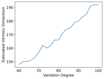
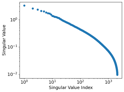
We conduct the above process with the variation degree $[98,96,94,92,90,88,86,84,82,80,78,76,74,72,70,68,66,64,62,60]$ utilized in the CIFAR10 experiments (see App. H). We additionally add a variation degree of 100 which is the highest variation degree in the API that was used to generate the initial samples. We plot the estimated intrinsic dimension v.s. variation degree in Fig. 9. The raw original singular values of $M/\sqrt{3000}$ for variation degree=60 are in Fig. 10 (other variation degrees have similar trend). Two key observations are:

• As the variation degree increases, the estimated intrinsic dimension also increases. This could be because the manifold of image embeddings is likely to be non-linear, the above estimation of intrinsic dimension is only accurate when we perturb the image $x$ to a small degree so that the changes in the manifold can still be well approximated by a linear subspace. Using a larger variation degree (and thus larger changes in the embedding space) will overestimate the intrinsic dimension.

• Nevertheless, we always see that the singular values decrease rapidly (Fig. 10) and the estimated intrinsic dimension is much smaller than the embedding size 2048 (Fig. 9), which supports our hypothesis in Thm. 2.

Figure 9: Estimated intrinsic dimension of inception embeddings of realistic images.

Figure 10: Singular values of inception embeddings of image variations at variation degree=60.

Appendix F Relation of DPWA to prior work

Recall that in DPWA, we want a DP algorithm to output $S_{\mathrm{syn}}$ which is close to the distribution of $S_{\mathrm{priv}}$ in Wasserstein distance w.r.t. some distance function $d(\cdot,\cdot)$. When the distance function $d(\cdot,\cdot)$ is just $\ell_{2}$ distance between the samples (i.e., $\ell_{2}$ in the pixel space for images), then DPWA is closely related to DP Clustering [26, 3, 51] and DP Heatmaps [25].

In [25], to give an algorithm for DP Heatmaps, the authors study DP sparse EMD aggregation problem where we need to output a distribution of points which approximates the distribution of private data in EMD distance (i.e., $W_{1}$). They study this problem only in two dimensions and the running time of their algorithms (suitably generalized to higher dimensions) will be exponential in the dimension $d$.

The DP Clustering problem requires us to output a clustering of private data using DP. The most common clustering studied is $k$-means clustering where we should output $k$ cluster centers such that $k$-means cost is minimized, where $k$-means cost is the sum of squares of $\ell_{2}$-distance of each data point to its nearest cluster center. Note that in DPWA, if the number of synthetic data points $N_{\mathrm{syn}}$ is specified to be $k$, then DP $k$-means clustering and DPWA with $W_{2}$ metric are equivalent. In [25], a polynomial time DP Clustering algorithm with an additional $k$-means cost (over what is non-privately possible) of $k\sqrt{d\log(1/\delta)}\mathrm{polylog}(N_{\mathrm{priv}},d)/\epsilon$ is given. This can be converted into an upper bound on the Wasserstein distance. But this is not a practical algorithm. The privacy-utility tradeoffs are bad due to the large hidden constants in the analysis and the authors don’t provide an implementation. There is a practical DP Clustering algorithm (along with an implementation) given in [13] (but with no theoretical guarantees).

F.1 Why Not Just Use DP Clustering?

We now explain why we can’t just use prior work on DP Clustering to solve DPSDA say for images.

Clustering in the image space. We can use DP $k$-means Clustering to cluster the images w.r.t. $\ell_{2}$ metric in the pixel space. This doesn’t work because $\ell_{2}$ distance in the pixel space doesn’t capture semantic similarity. An image which is slightly shifted in pixel space gets very far in $\ell_{2}$ distance. And the dimension of the images is too large for prior DP Clustering algorithms to work well. Their convergence and privacy-utility tradeoffs depend too strongly on the dimension.

Clustering in the embedding space. We can use DP $k$-means Clustering to cluster the image embeddings w.r.t. $\ell_{2}$ metric in the embedding space. Note that this is the distance function we use in PE (Eq. 1). Even after we find the cluster centers, it is hard to invert the embedding map (i.e., find an image whose embedding is close to a given vector in the embedding space). Moreover the dimension of the embedding space is still too large for the above methods to be practical.

Our PE algorithm does much better because:

1. Its distance function is $\ell_{2}$ in the embedding space which captures semantic similarity,

2. It exploits the intrinsic dimension of the manifold of images in the embedding space which is much smaller than the embedding dimension (see Thm. 2 and App. E) and

3. There is no need to invert points in embedding space to the image space.

In an early experiment, we have tried DP clustering in the CLIP embedding space using the practical DP Clustering algorithm in [13]. We then inverted the cluster centers (which are in the embedding space) using unCLIP. But we found the resulting images are too noisy compared to the images we get from PE and the FID scores are also significantly worse than that of PE.

Appendix G Implementation Details on Label Condition

There are two meanings of “conditioning” that appear in our work:

• Whether the pre-trained networks or APIs (e.g., ImageNet pre-trained diffusion models used in § 6.1.1 and 6.1.2) support conditional input (e.g., ImageNet class label).

• Whether the generated samples are associated with class labels from the private data.

In DP fine-tuning approaches, these two usually refer to the same thing: if we want to generate class labels for generated samples, the common practice is to use a pre-trained network that supports conditional input [24]. However, in PE, these two are completely orthogonal.

Conditional pre-trained networks/APIs. We first explain our implementation when the pre-trained networks or APIs support conditional inputs such as class labels or text prompts. When generating the initial population using RANDOM_API (Alg. 1), we will either randomly draw labels from all possible labels when no prior public information is available (which is what we do in CIFAR10 and Camelyon17 experiments where we randomly draw from all possible ImageNet classes), or use the public information as condition input (e.g., the text prompt used in Stable Diffusion experiments; see App. J). In the subsequent VARIATION_API calls (Alg. 1), for each image, we will use its associated class label or text prompt as the condition information to the API, and the output samples from VARIATION_API will be associated with the same class label or text prompt as the input sample. For example, if we use an image with “peacock” class to generate variations, all output images will be associated with “peacock” class for future VARIATION_API calls. Note that throughout the above process, all the condition inputs to the pre-trained networks/APIs are public information; they have nothing to do with the private classes.

Conditional generation. Conditional generation is achieved by Alg. 3, where we separate the samples according to their class labels, and run the main algorithm (Alg. 1) on each sample set. We can use either conditional or unconditional pre-trained networks/APIs to implement it.

Throughout the paper, “(un)condition” refers to 2, expect the caption in Fig. 8 which refers to 1.

Appendix H More Details on CIFAR10 Experiments

Pre-trained model. By default, we use the checkpoint imagenet64_cond_270M_250K.pt released in [43]. For the ablation study of the pre-trained network, we additionally use the checkpoint imagenet64_uncond_100M_1500K.pt.

API implementation. RANDOM_API follows the standard diffusion model sampling process. VARIATION_API is implemented with SDEdit [42], which adds noise to input images and lets the diffusion model to denoise. We use DDIM sampler [50] and the default noise schedule to draw samples. Note that these choices are not optimal; our results can potentially be improved by using better noise schedules and the full DDPM sampling [34] which are known to work better. The implementation of the above APIs is straightforward without touching the core modeling part of diffusion models and is similar to the standard API implementations in Stable Diffusion (App. J).

Hyperparameters. We set number of iterations $T=20$, lookahead degree $k=8$, and number of generated samples $N_{\mathrm{syn}}=50000$. For RANDOM_API and VARIATION_API, we use DDIM sampler with 100 steps. For VARIATION_API, we use SDEEdit [42] by adding noise till $[98,96,94,92,90,88,86,84,82,80,78,76,74,72,70,68,66,64,62,60]$ timesteps for each iteration respectively. These timesteps can be regarded as the $v$ parameter in § 3.3.

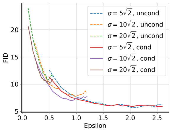
For the experiments in Fig. 4, we use noise multiplier $\sigma=t\cdot\sqrt{2}$ and threshold $H=2t$ for $t\in\left\{5,10,20\right\}$, and pick the the pareto frontier. Fig. 11 shows all the data points we got. Combining this figure with Fig. 4, we can see that PE is not very sensitive to these hyper-parameters, and even with less optimal choices PE still outperforms the baselines.

Figure 11: FID (lower is better) v.s. privacy cost $\epsilon$ ($\delta=10^{-5}$) on CIFAR10 with different noise multipliers and thresholds. “(Un)cond” means (un)conditional generation.

For the experiments in Fig. 5, we use noise multiplier $\sigma=\sqrt{2}$ and threshold $H=2$.

For downstream classification (Fig. 5), we follow [24] to use WRN-40-4 classifier [58]. We use the official repo without changing any hyper-parameter except adding color jitter augmentation according to [24]. The ensemble of the classifier is implemented by ensembling the logits.

FID evaluation. Compared to Fig. 4 in the main text, Fig. 12 shows the full results of two versions of [31]. Baseline results are taken from [31, 24].

Figure 12: FID [33] (lower is better) v.s. privacy cost $\epsilon$ on CIFAR10 ($\delta=10^{-5}$). Baseline results are taken from [31, 24]. (Un)cond means (un)conditional generation. Ours achieves the best privacy-quality trade-off.

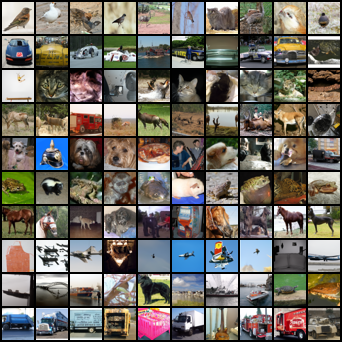
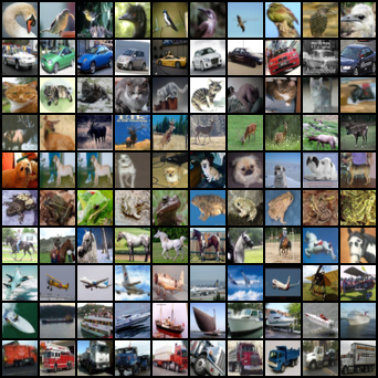
Generated samples. See Figs. 14 and 14 for generated images and real images side-by-side. Note that the pre-trained model we use generates 64x64 images, whereas CIFAR10 is 32x32. In Fig. 4, we show the raw generated 64x64 images; in Fig. 14, we scale them down to 32x32 for better comparison with the real images.

Figure 13: Generated samples on CIFAR10 with $\left(0.67,10^{-5}\right)$-DP. Each row corresponds to one class. FID=7.87.

Figure 14: Real samples from CIFAR10. Each row corresponds to one class.

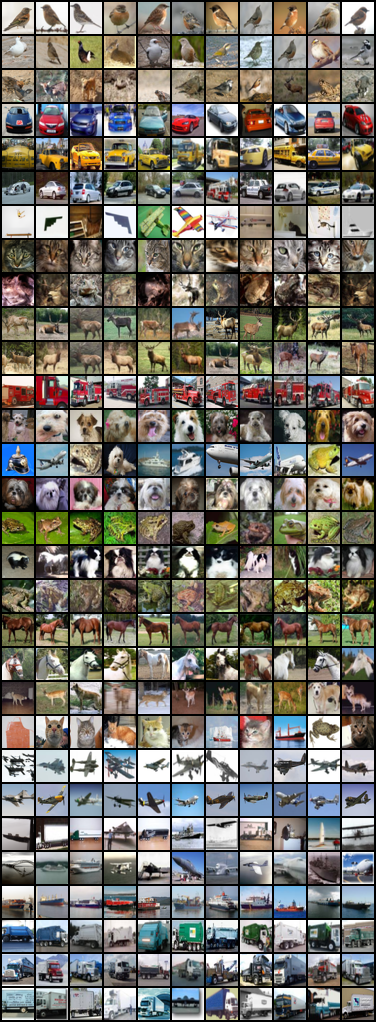
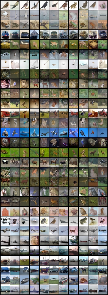
Nearest samples in the private dataset Figs. 15 and 16 show generated images and their nearest neighbors in the private dataset evaluated using two distance metrics: $\ell_{2}$ distance in the inception embedding space and the pixel space. We can see that the generated images are different from private images. This is expected due to the DP guarantee.

Figure 15: Nearest samples in the private dataset on CIFAR10. In each row, the first column is a generated image (from Fig. 14), and the other columns are its nearest neighbors in the private dataset, sorted by the distance in ascending order. Every three rows correspond to generated image from one class. The distance metric is $\ell_{2}$ in the inception embedding space.

Figure 16: Nearest samples in the private dataset on CIFAR10. In each row, the first column is a generated image (from Fig. 14), and the other columns are its nearest neighbors in the private dataset, sorted by the distance in ascending order. Every three rows correspond to generated image from one class. The distance metric is $\ell_{2}$ in the pixel space.

Appendix I More Details on Camelyon17 Experiments

Pre-trained model. We use the checkpoint imagenet64_cond_270M_250K.pt released in [43].

API implementation. Same as App. H.

Hyperparameters. We set lookahead degree $k=8$, and number of generated samples $N_{\mathrm{syn}}=302436$.

About the experiments in Fig. 18. For RANDOM_API and VARIATION_API, we use DDIM sampler with 10 steps. For VARIATION_API, we take a 2-stage approach. the first stage, we use DDIM sampler with 10 steps and use SDEEdit [42] by adding noise till $[10,10,10,10,9,9,9,9,9,8,8,8,8,8,7,7,7,7]$ timesteps for each iteration respectively. In the second stage, we use DDIM sampler with 40 steps and use SDEEdit [42] by adding noise till $[20,19,18,17,16,15,14,13,12,11,10,9,8,7,6,5]$ timesteps for each iteration respectively. These timesteps can be regarded as the $v$ parameter in § 3.3. We use noise multiplier $\sigma=2\cdot\sqrt{2}$ and threshold $H=4$.

About the experiments in § 6.1.2. For RANDOM_API and VARIATION_API, we use DDIM sampler with 10 steps. For VARIATION_API, we use DDIM sampler with 10 steps and use SDEEdit [42] by adding noise till $[10,10,10,10,9,9,9,9,9,8,8,8,8,8,7,7,7,7,7]$ timesteps for each iteration respectively. These timesteps can be regarded as the $v$ parameter in § 3.3. We use noise multiplier $\sigma=1.541\cdot\sqrt{2}$ and threshold $H=4$.

Generated samples. See Figs. 18 and 18 for generated images and real images side-by-side. Note that the real images in Camelyon17 dataset are 96x96 images, whereas the pre-trained network is 64x64. In Fig. 18, we scale them down to 64x64 for better comparison.

Fig. 19 shows the generated images in the intermediate iterations. We can see that the generated images are effectively guided towards Camelyon17 though it is very different from the pre-training dataset.

Figure 17: Generated samples on Camelyon17 with $\left(9.92,3\cdot 10^{-6}\right)$-DP. The first five rows correspond to one class, and the rest correspond to the other class. FID=10.66.

Figure 18: Real samples from Camelyon17. The first five rows correspond to one class, and the rest correspond to the other class.

(a) Iteration=1.

(b) Iteration=3.

(c) Iteration=5.

(d) Iteration=7.

(e) Iteration=9.

(f) Iteration=11.

(g) Iteration=13.

(h) Iteration=15.

(i) Iteration=17.

(j) Iteration=19.

(k) Iteration=21.

(l) Iteration=23.

Figure 19: Generated samples on Camelyon17 at the first few iterations. We can see that the generated images are gradually guided from ImageNet, the pre-training dataset, to Camelyon17, the (very different) private dataset.

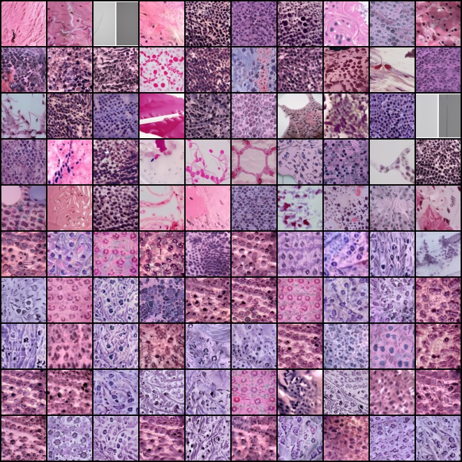
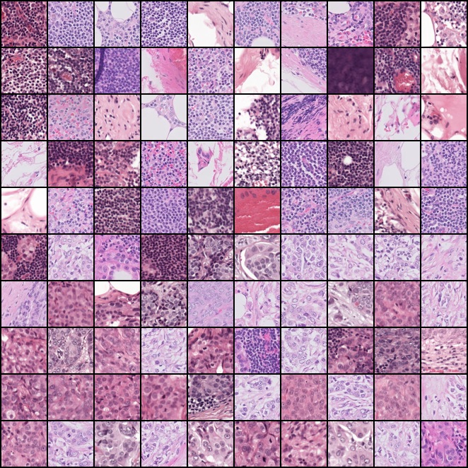
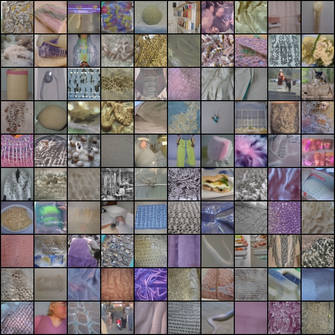
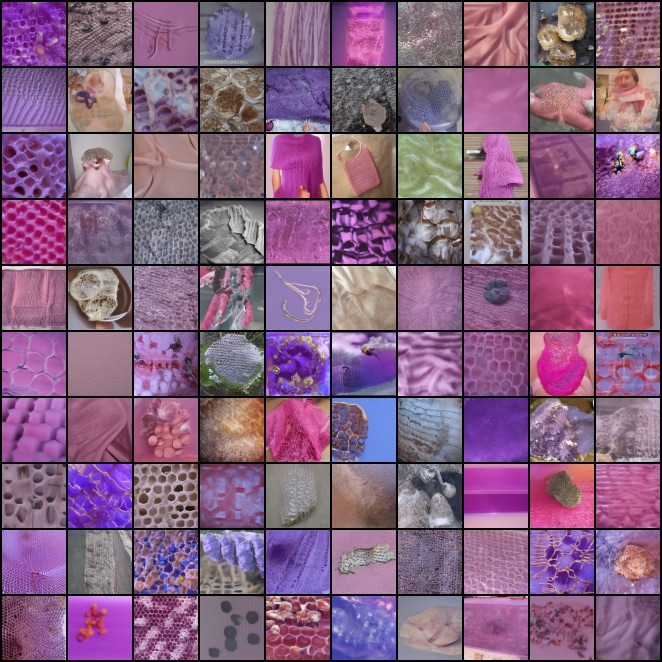
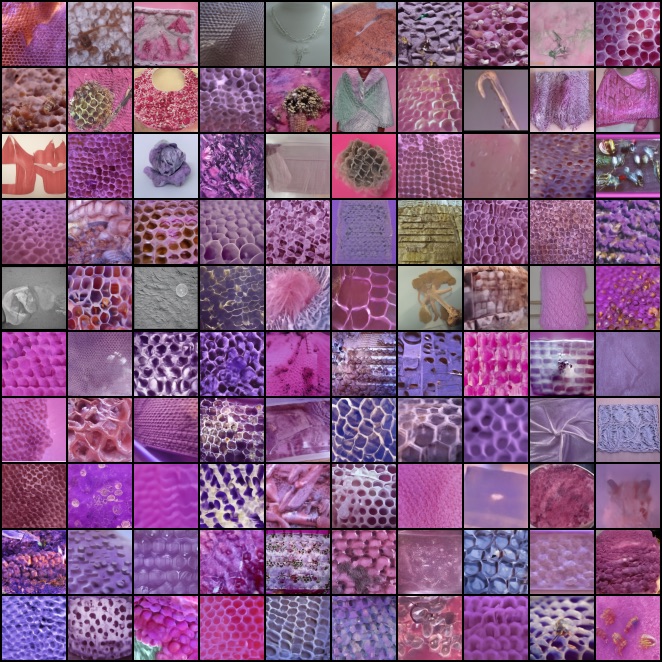
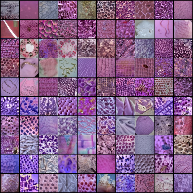
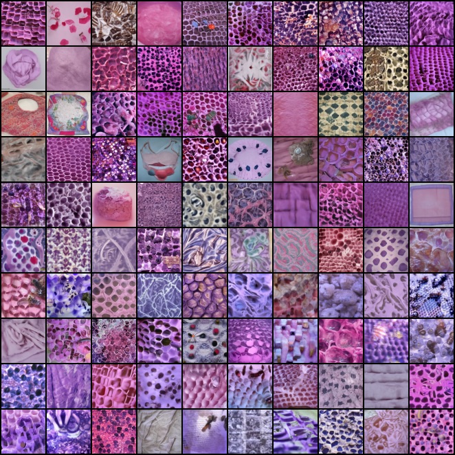
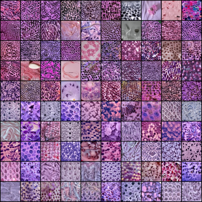
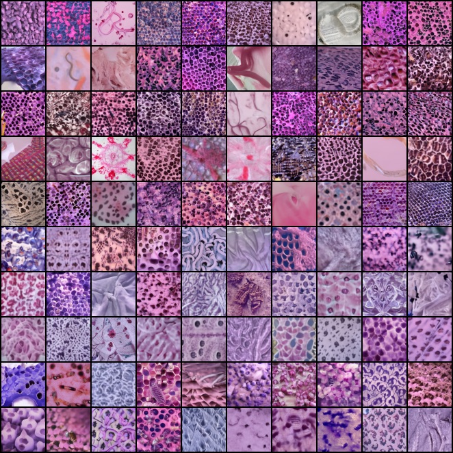
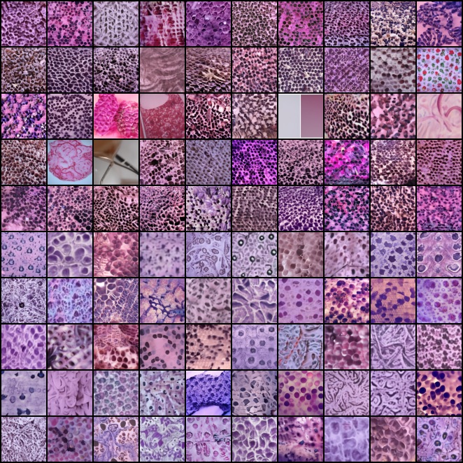
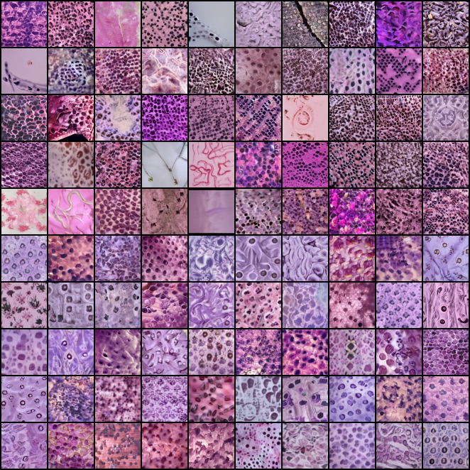
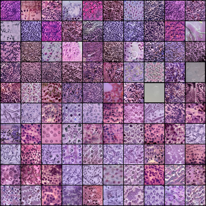
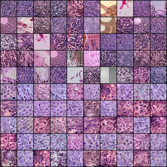
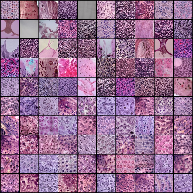
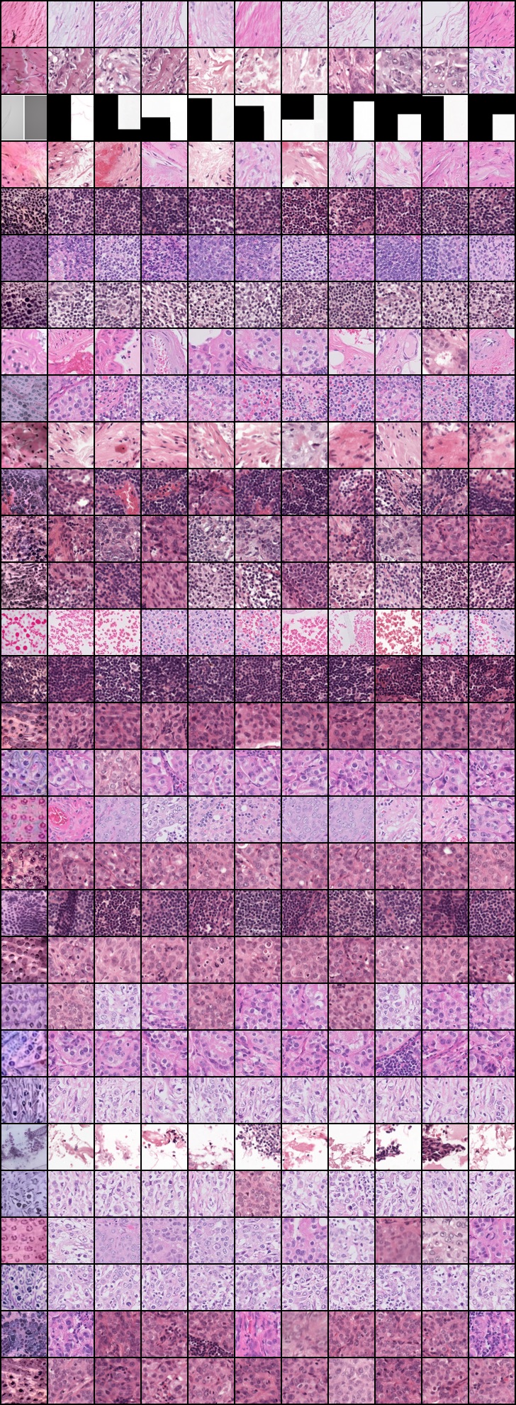
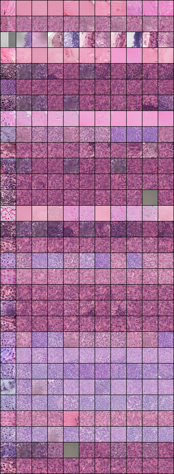
Nearest samples in the private dataset Figs. 20 and 21 show generated images and their nearest neighbors in the private dataset evaluated using two distance metrics: $\ell_{2}$ distance in the inception embedding space and the pixel space. Similar to the results in CIFAR10, we can see that the generated images are different from private images. This is expected due to the DP guarantee.

Figure 20: Nearest samples in the private dataset on Camelyon17. In each row, the first column is a generated image (from Fig. 18), and the other columns are its nearest neighbors in the private dataset, sorted by the distance in ascending order. Every fifteen rows correspond to generated image from one class. The distance metric is $\ell_{2}$ in the inception embedding space.

Figure 21: Nearest samples in the private dataset on Camelyon17. In each row, the first column is a generated image (from Fig. 14), and the other columns are its nearest neighbors in the private dataset, sorted by the distance in ascending order. Every fifteen rows correspond to generated image from one class. The distance metric is $\ell_{2}$ in the pixel space.

Appendix J More Details on Stable Diffusion Experiments

Dataset construction. We start with cat photos taken by the authors, crop the region around cat faces with a resolution larger than 512x512 manually, and resize the images to 512x512. We construct two datasets, each for one cat with 100 images. See Figs. 22 and 23 for all images.

Figure 22: All images from Cat Cookie dataset. The original resolution is 512x512; we resize them to 128x128 here for reducing the file size of the paper.

Figure 23: All images from Cat Doudou dataset. The original resolution is 512x512; we resize them to 128x128 here for reducing the file size of the paper.

API implementation. We use off-the-shelf open-sourced APIs of Stable Diffusion. For RANDOM_API, we use the text-to-image generation API, which is implemented by the standard diffusion models’ guided sampling process. For VARIATION_API, we use the image-to-image generation API, which allows us to control the degree of variation. Its internal implementation is SDEdit [42], which adds noise to the input images and runs diffusion models’ denoising process.

Hyperparameters We set lookahead degree $k=8$, and number of generated samples $N_{\mathrm{syn}}=100$. For RANDOM_API and VARIATION_API, we use the default DDIM sampler with 50 steps. For RANDOM_API, we use the prompt "A photo of ragdoll cat". This gives reaonable cat images but still far away from the private data (Fig. 26). For VARIATION_API, we use variation degrees $[0.98,0.96,0.94,0.92,0.90,0.88,0.84,0.8,0.76,0.72,0.68,0.64,0.6]$ for each iteration respectively with the same prompt. We use noise multiplier $\sigma=2$ and threshold $H=2$. We use inception embedding for Eq. 1.

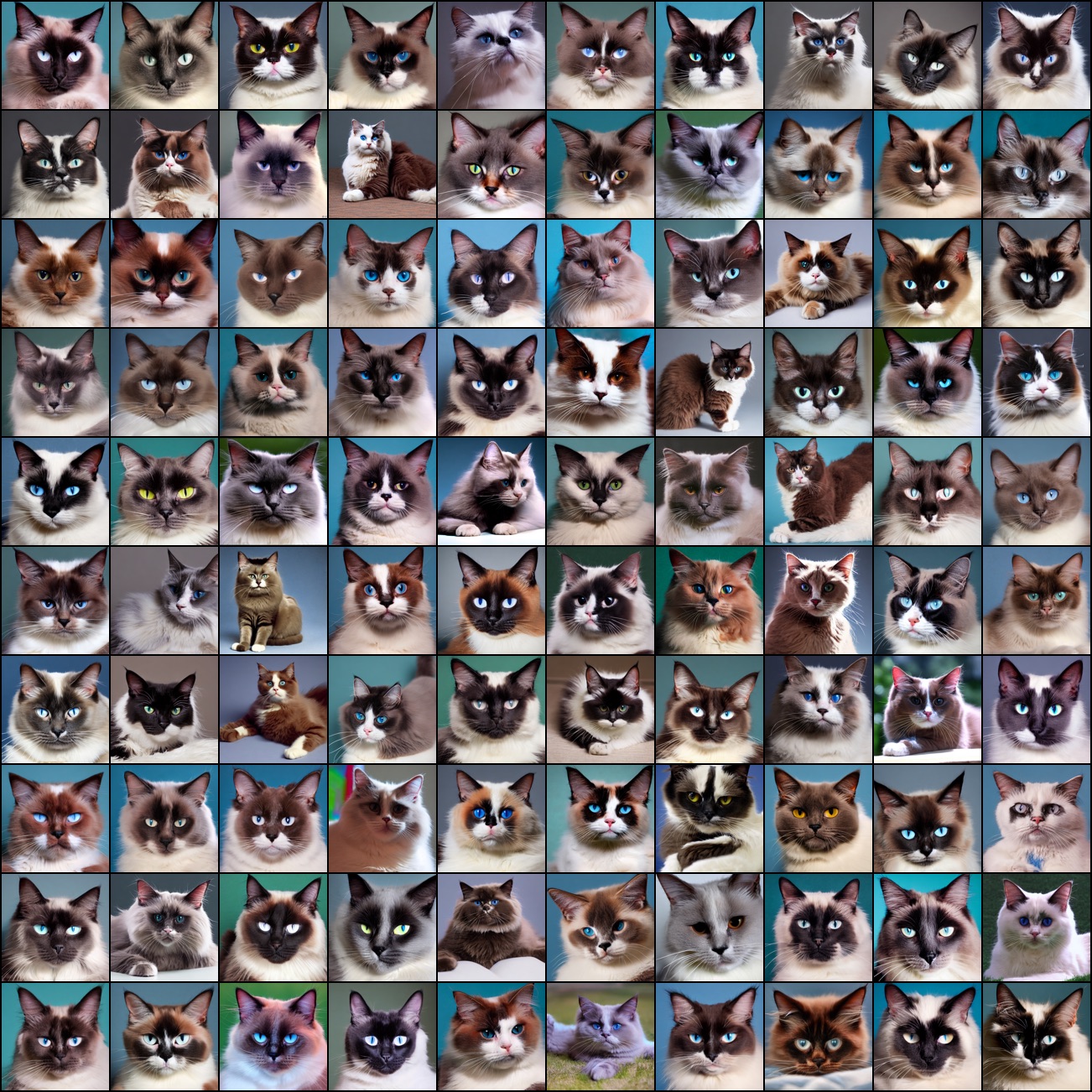
Generated images. We use the same hyper-parameters to run PE on two datasets separately. This can also be regarded as running the conditional version of PE (Alg. 3) on the whole dataset (with labels Cat Cookie or Cat Doudou) together. All generated images are in Figs. 24 and 25. While the two experiments use completely the same hyper-parameters, and the initial random images are very different from the cats (Fig. 26), our PE can guide the generated distribution in the right direction and the final generated images do capture the key color and characteristics of each of the cats. This demonstrates the effectiveness of PE with large foundation models such as Stable Diffusion.

We also observe that the diversity of generated images (e.g., poses, face directions) is limited compared to the real data. However, given the small number of samples and the tight privacy budget, this is an expected behavior: capturing more fine-grained features of each image would likely violate DP.

Figure 24: All generated images from Cat Cookie dataset with $(6.62,10^{-3})$-DP. The original resolution is 512x512; we resize them to 128x128 here for reducing the file size of the paper.

Figure 25: All generated images from Cat Doudou dataset with $(6.62,10^{-3})$-DP. The original resolution is 512x512; we resize them to 128x128 here for reducing the file size of the paper.

Figure 26: The initial random images from Stable Diffusion. The original resolution is 512x512; we resize them to 128x128 here for reducing the file size of the paper.

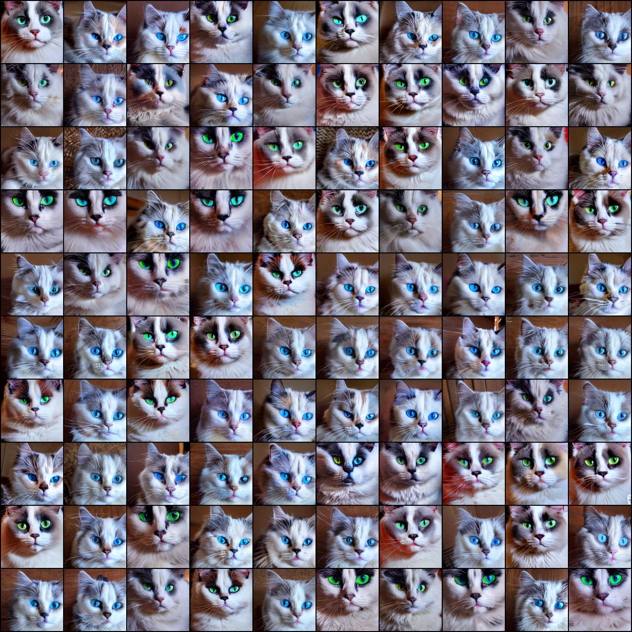
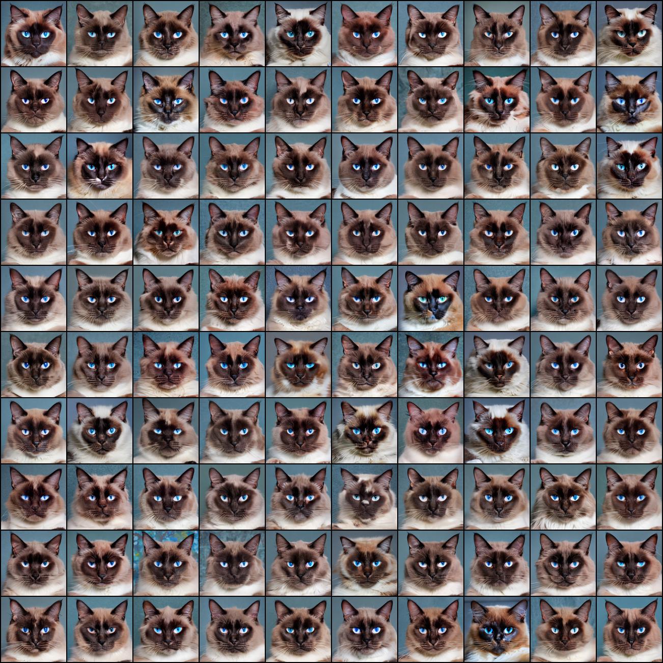
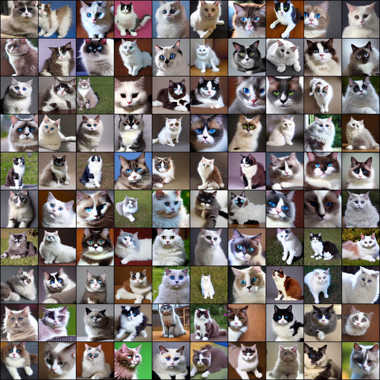
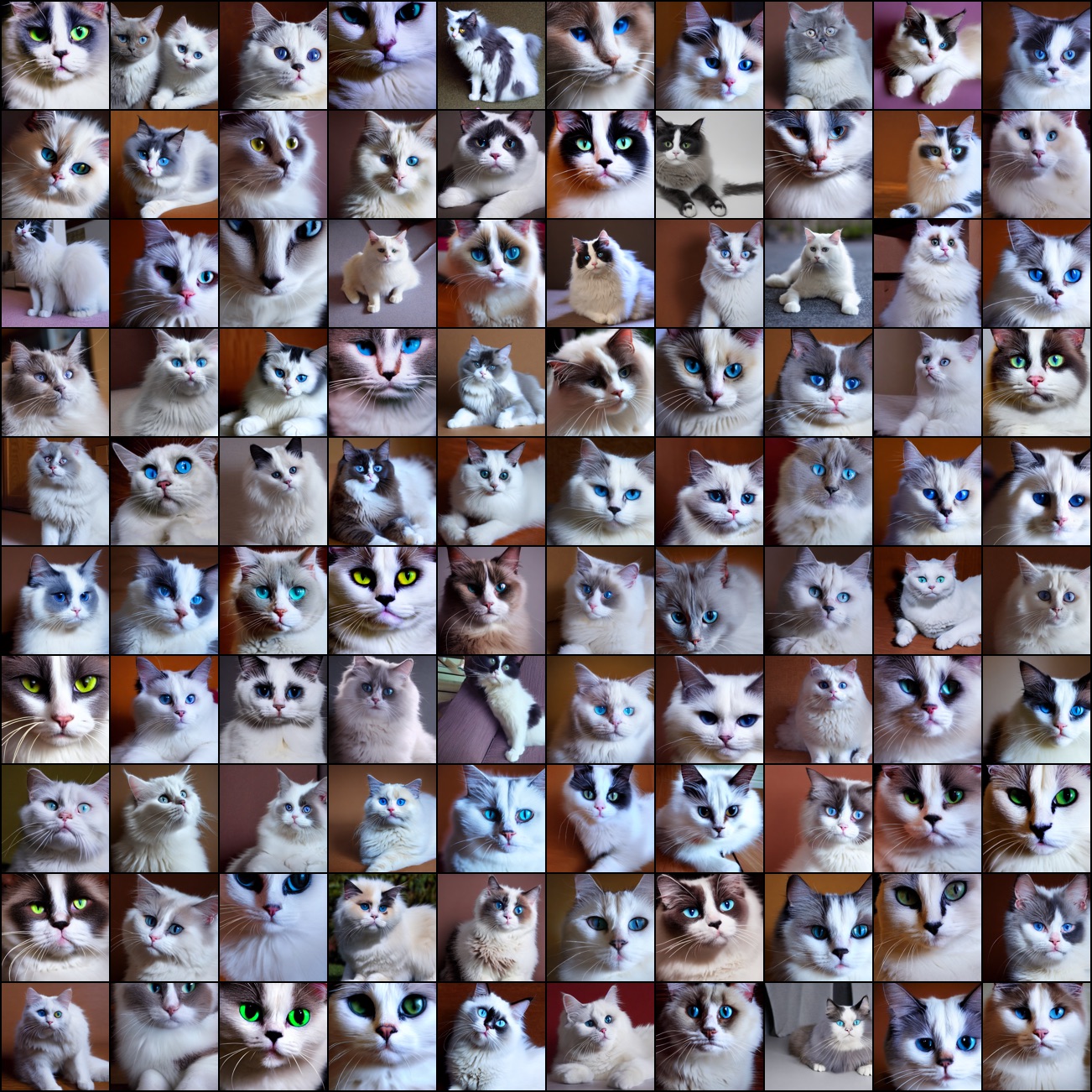
Generated images with more diversity. To make the generated images more diverse, we can utilize the approach in § 4.1, which passes the generated images through VARIATION_API. We have demonstrated in § 6.1.3 that this approach can generate more samples that are useful for downstream classification tasks. Here, we use it for a different purpose: enriching the diversity of generated samples.

Figure Figs. 27 and 28 show the results. We can see that this simple approach is able to generate cats with a more diverse appearance. This is possible because the foundation model (Stable Diffusion) has good prior knowledge about cats learned from massive pre-training, and PE is able to utilize that effectively.

Figure 27: Generated images with enhanced diversity using the approach in § 4.1 on Cat Cookie. The original resolution is 512x512; we resize them to 128x128 here for reducing the file size of the paper.

Figure 28: Generated images with enhanced diversity using the approach in § 4.1 on Cat Doudou. The original resolution is 512x512; we resize them to 128x128 here for reducing the file size of the paper.

Appendix K More Ablation Studies

All ablation studies are conducted by taking the default parameters in unconditional CIFAR10 experiments and modifying one hyperparameter at a time. The default noise multiplier $\sigma=5\cdot\sqrt{2}$ and the default threshold $H=10$.

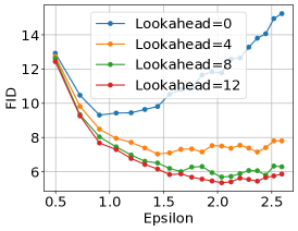
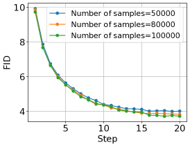
Lookahead degree. Fig. 29 shows how the lookahead degree $k$ (§ 4) impacts the results. We can see that higher lookahead degrees monotonically improve the FID score. Throughout all experiments, we used $k=8$. This experiment suggests that better results can be obtained with a higher $k$.

Figure 29: Ablation studies on the lookahead degree $k$ for DP Nearest Neighbors Histogram. Lookahead=0 means lookahead is not used (Eq. 1).

Population size. Fig. 30 shows how the number of generated samples $N_{\mathrm{syn}}$ impacts the results in non-DP setting. We can see that, as the number of samples increases, FID score monotonically gets better. This is expected because with more generated samples, there are higher chances to get samples similar to the private data. However, we want to point out that in the DP case, it may not be true, as a large number of samples would flatten the DP Nearest Neighbors Histogram and thus decrease the signal noise ratio.

Figure 30: Ablation studies on the number of generated samples $N_{\mathrm{syn}}$ in non-DP setting.

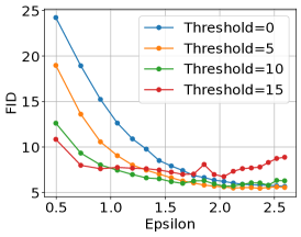
Histogram threshold. Fig. 31 shows how the threshold $H$ in DP Nearest Neighbors Histogram impacts the results. We can see that a large threshold results in a faster convergence speed at the beginning. This is because, in the early iterations, many samples are far away from the private data. A larger threshold can effectively remove those bad samples that have a non-zero histogram count due to the added DP noise. However, at a later iteration, the distribution of generated samples is already close to the private data. A large threshold may potentially remove useful samples (e.g., the samples at low-density regions such as classifier boundaries). This may hurt the generated data, as shown in the increasing FID scores at threshold=15. In this paper, we used a fixed threshold across all iterations. These results suggest that an adaptive threshold that gradually decreases might work better.

Figure 31: Ablation studies on the threshold $H$ for DP Nearest Neighbors Histogram.

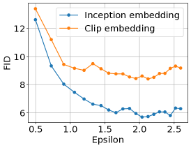
Embedding. Fig. 32 compares the results with inception embedding or CLIP embedding in Eq. 1. The results show that both embedding networks work well, suggesting that PE is not too sensitive to the embedding network. Inception embedding works slightly better. One reason is that the inception network is trained on ImageNet, which is similar to a private dataset (CIFAR10). Therefore, it might be better at capturing the properties of images. Another possible reason is that FID score is calculated using inception embeddings, which might lead to some bias that favors inception embedding.

Figure 32: Ablation studies on the embedding network in Eq. 1 to use.

Appendix L Computational Cost Evaluation

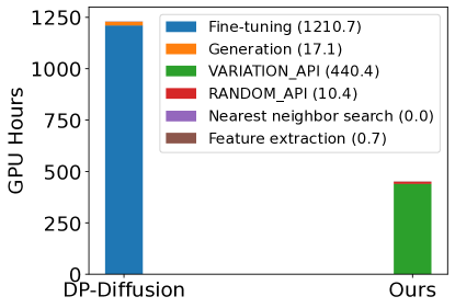
We compare the GPU hours of the SOTA DP fine-tuning method [24] and PE for generating 50k samples in § 6.1.1. Note that PE is designed to use existing pre-trained models and we do so in all experiments. In contrast, DP fine-tuning methods usually require a careful selection of pre-training datasets and architectures (e.g., [24] pre-trained their own diffusion models), which could be costly. Even if we ignore this and only consider the computational cost after the pre-training, the total computational cost of PE is only 37% of [24] while having better sample quality and downstream classification accuracy (§ 6.1.1). See Fig. 33 for a detailed breakdown of the computational cost. Note that PE’s computational cost is mostly on the APIs.

The key takeaway is that even if practitioners want to run the APIs locally (i.e., downloading the foundation models and running the APIs locally without using public API providers), there are still benefits of using PE: (1) The computational cost of PE can be smaller than training-based methods. (2) Implementing and deploying PE are easier because PE only requires blackbox APIs of the models and does not require code modifications inside the models.

Experimental details. To ensure a fair comparison, we estimate the runtime of both algorithms using 1 NVIDIA V100 32GB GPU.

To evaluate the computational cost of [24], we take the open-source diffusion model implementation from [17] and modify the hyper-parameters according to [24]. We obtain a model with 79.9M parameters, slightly smaller than the one reported in [24] (80.4M). This difference might be due to other implementation details that are not mentioned in [24]. To implement DP training, we utilize Opacus library [55]. To evaluate the fine-tuning cost, we use torch.cuda.Event instrumented before and after the core logic of forward and backward pass, ignoring other factors such as data loading time. We estimate the total runtime based on the mean runtime of 10 batches after 10 batches of warmup. We do not implement augmentation multiplicity with data and timestep [24]; instead, we use multiplicity=1 (i.e., a vanilla diffusion model), and multiply the estimated runtime by 128, the multiplicity used in [24]. To evaluate the generation cost, we use torch.cuda.Event instrumented before and after the core logic of sampling. We estimate the total runtime based on the mean runtime of 10 batches after 1 batch of warmup.

To evaluate the computational cost of our PE, we use a similar method: we use torch.cuda.Event instrumented before and after the core logic of each component of our algorithm that involves GPU computation. RANDOM_API and VARIATION_API are estimated based on the mean runtime of 10 batches after 1 batch of warmup. Feature extraction is estimated based on the mean runtime of 90 batches after 10 batch of warmup. The nearest neighbor search is estimated based on 1 run of the full search. We use faiss library for nearest neighbor search. Its implementation is very efficient so its computation time is negligible compared with the total time.

Figure 33: GPU hours (on 1 NVIDIA V100 32GB) required to obtain the samples for § 6.1.1 with DP-Diffusion [24] and ours. The legend denotes the steps and the GPU hours; [24] contains the fine-tuning and generation steps, whereas ours contains the other steps.

References

- [1] Martin Abadi, Andy Chu, Ian Goodfellow, H Brendan McMahan, Ilya Mironov, Kunal Talwar, and Li Zhang. Deep learning with differential privacy. In Proceedings of the 2016 ACM SIGSAC conference on computer and communications security, pages 308–318, 2016.
- [2] Martin Arjovsky, Soumith Chintala, and Léon Bottou. Wasserstein generative adversarial networks. In International conference on machine learning, pages 214–223. PMLR, 2017.
- [3] Maria-Florina Balcan, Travis Dick, Yingyu Liang, Wenlong Mou, and Hongyang Zhang. Differentially private clustering in high-dimensional euclidean spaces. In International Conference on Machine Learning, pages 322–331. PMLR, 2017.
- [4] Borja Balle and Yu-Xiang Wang. Improving the gaussian mechanism for differential privacy: Analytical calibration and optimal denoising. In International Conference on Machine Learning, pages 394–403. PMLR, 2018.
- [5] Peter Bandi, Oscar Geessink, Quirine Manson, Marcory Van Dijk, Maschenka Balkenhol, Meyke Hermsen, Babak Ehteshami Bejnordi, Byungjae Lee, Kyunghyun Paeng, Aoxiao Zhong, et al. From detection of individual metastases to classification of lymph node status at the patient level: the camelyon17 challenge. IEEE transactions on medical imaging, 38(2):550–560, 2018.
- [6] Brett K Beaulieu-Jones, Zhiwei Steven Wu, Chris Williams, Ran Lee, Sanjeev P Bhavnani, James Brian Byrd, and Casey S Greene. Privacy-preserving generative deep neural networks support clinical data sharing. Circulation: Cardiovascular Quality and Outcomes, 12(7):e005122, 2019.
- [7] Tom Brown, Benjamin Mann, Nick Ryder, Melanie Subbiah, Jared D Kaplan, Prafulla Dhariwal, Arvind Neelakantan, Pranav Shyam, Girish Sastry, Amanda Askell, et al. Language models are few-shot learners. Advances in neural information processing systems, 33:1877–1901, 2020.
- [8] Nicholas Carlini, Steve Chien, Milad Nasr, Shuang Song, Andreas Terzis, and Florian Tramer. Membership inference attacks from first principles. arXiv preprint arXiv:2112.03570, 2021.
- [9] Nicholas Carlini, Jamie Hayes, Milad Nasr, Matthew Jagielski, Vikash Sehwag, Florian Tramer, Borja Balle, Daphne Ippolito, and Eric Wallace. Extracting training data from diffusion models. arXiv preprint arXiv:2301.13188, 2023.
- [10] Nicholas Carlini, Daphne Ippolito, Matthew Jagielski, Katherine Lee, Florian Tramer, and Chiyuan Zhang. Quantifying memorization across neural language models. International Conference on Learning Representations, 2023.
- [11] Nicholas Carlini, Chang Liu, Úlfar Erlingsson, Jernej Kos, and Dawn Song. The secret sharer: Evaluating and testing unintended memorization in neural networks. In 28th USENIX Security Symposium, 2019.
- [12] Nicholas Carlini, Florian Tramèr, Eric Wallace, Matthew Jagielski, Ariel Herbert-Voss, Katherine Lee, Adam Roberts, Tom Brown, Dawn Song, Ulfar Erlingsson, Alina Oprea, and Colin Raffel. Extracting training data from large language models. In 30th USENIX Security Symposium, USENIX Security ’21, pages 2633–2650. USENIX Association, 2021.
- [13] Alisa Chang and Pritish Kamath. Differentially private clustering in google’s differential privacy library. Google AI Blog, 2023. https://ai.googleblog.com/2021/10/practical-differentially-private.html.
- [14] Christopher A Choquette-Choo, Florian Tramer, Nicholas Carlini, and Nicolas Papernot. Label-only membership inference attacks. In Proceedings of the 38th International Conference on Machine Learning, ICML ’21, pages 1964–1974. JMLR, Inc., 2021.
- [15] Lawrence Davis. Genetic algorithms and simulated annealing. 1987.
- [16] Jia Deng, Wei Dong, Richard Socher, Li-Jia Li, Kai Li, and Li Fei-Fei. Imagenet: A large-scale hierarchical image database. In 2009 IEEE conference on computer vision and pattern recognition, pages 248–255. Ieee, 2009.
- [17] Prafulla Dhariwal and Alexander Nichol. Diffusion models beat gans on image synthesis. Advances in Neural Information Processing Systems, 34:8780–8794, 2021.
- [18] Tim Dockhorn, Tianshi Cao, Arash Vahdat, and Karsten Kreis. Differentially private diffusion models. arXiv preprint arXiv:2210.09929, 2022.
- [19] Jinshuo Dong, Aaron Roth, and Weijie J Su. Gaussian differential privacy. Journal of the Royal Statistical Society Series B: Statistical Methodology, 84(1):3–37, 2022.
- [20] Cynthia Dwork, Frank McSherry, Kobbi Nissim, and Adam Smith. Calibrating noise to sensitivity in private data analysis. In Theory of Cryptography: Third Theory of Cryptography Conference, TCC 2006, New York, NY, USA, March 4-7, 2006. Proceedings 3, pages 265–284. Springer, 2006.
- [21] Cynthia Dwork, Aaron Roth, et al. The algorithmic foundations of differential privacy. Foundations and Trends® in Theoretical Computer Science, 9(3–4):211–407, 2014.
- [22] Matt Fredrikson, Somesh Jha, and Thomas Ristenpart. Model inversion attacks that exploit confidence information and basic countermeasures. In Proceedings of the 22nd ACM SIGSAC conference on computer and communications security, pages 1322–1333, 2015.
- [23] Arun Ganesh, Mahdi Haghifam, Milad Nasr, Sewoong Oh, Thomas Steinke, Om Thakkar, Abhradeep Thakurta, and Lun Wang. Why is public pretraining necessary for private model training? arXiv preprint arXiv:2302.09483, 2023.
- [24] Sahra Ghalebikesabi, Leonard Berrada, Sven Gowal, Ira Ktena, Robert Stanforth, Jamie Hayes, Soham De, Samuel L Smith, Olivia Wiles, and Borja Balle. Differentially private diffusion models generate useful synthetic images. arXiv preprint arXiv:2302.13861, 2023.
- [25] Badih Ghazi, Junfeng He, Kai Kohlhoff, Ravi Kumar, Pasin Manurangsi, Vidhya Navalpakkam, and Nachiappan Valliappan. Differentially private heatmaps. arXiv preprint arXiv:2211.13454, 2022.
- [26] Badih Ghazi, Ravi Kumar, and Pasin Manurangsi. Differentially private clustering: Tight approximation ratios. Advances in Neural Information Processing Systems, 33:4040–4054, 2020.
- [27] Ian Goodfellow, Jean Pouget-Abadie, Mehdi Mirza, Bing Xu, David Warde-Farley, Sherjil Ozair, Aaron Courville, and Yoshua Bengio. Generative adversarial networks. Communications of the ACM, 63(11):139–144, 2020.
- [28] Sivakanth Gopi, Pankaj Gulhane, Janardhan Kulkarni, Judy Hanwen Shen, Milad Shokouhi, and Sergey Yekhanin. Differentially private set union. In International Conference on Machine Learning, pages 3627–3636. PMLR, 2020.
- [29] Niv Haim, Gal Vardi, Gilad Yehudai, Ohad Shamir, and Michal Irani. Reconstructing training data from trained neural networks. arXiv preprint arXiv:2206.07758, 2022.
- [30] Frederik Harder, Kamil Adamczewski, and Mijung Park. Dp-merf: Differentially private mean embeddings with randomfeatures for practical privacy-preserving data generation. In International conference on artificial intelligence and statistics, pages 1819–1827. PMLR, 2021.
- [31] Frederik Harder, Milad Jalali, Danica J Sutherland, and Mijung Park. Pre-trained perceptual features improve differentially private image generation. Transactions on Machine Learning Research, 2023.
- [32] Jiyan He, Xuechen Li, Da Yu, Huishuai Zhang, Janardhan Kulkarni, Yin Tat Lee, Arturs Backurs, Nenghai Yu, and Jiang Bian. Exploring the limits of differentially private deep learning with group-wise clipping. arXiv preprint arXiv:2212.01539, 2022.
- [33] Martin Heusel, Hubert Ramsauer, Thomas Unterthiner, Bernhard Nessler, and Sepp Hochreiter. Gans trained by a two time-scale update rule converge to a local nash equilibrium. Advances in neural information processing systems, 30, 2017.
- [34] Jonathan Ho, Ajay Jain, and Pieter Abbeel. Denoising diffusion probabilistic models. Advances in Neural Information Processing Systems, 33:6840–6851, 2020.
- [35] James Jordon, Jinsung Yoon, and Mihaela Van Der Schaar. PATE-GAN: Generating synthetic data with differential privacy guarantees. In International conference on learning representations, 2019.
- [36] Pang Wei Koh, Shiori Sagawa, Henrik Marklund, Sang Michael Xie, Marvin Zhang, Akshay Balsubramani, Weihua Hu, Michihiro Yasunaga, Richard Lanas Phillips, Irena Gao, et al. Wilds: A benchmark of in-the-wild distribution shifts. In International Conference on Machine Learning, pages 5637–5664. PMLR, 2021.
- [37] Alex Krizhevsky, Geoffrey Hinton, et al. Learning multiple layers of features from tiny images. 2009.
- [38] Xuechen Li, Daogao Liu, Tatsunori B Hashimoto, Huseyin A Inan, Janardhan Kulkarni, Yin-Tat Lee, and Abhradeep Guha Thakurta. When does differentially private learning not suffer in high dimensions? Advances in Neural Information Processing Systems, 35:28616–28630, 2022.
- [39] Xuechen Li, Florian Tramer, Percy Liang, and Tatsunori Hashimoto. Large language models can be strong differentially private learners. arXiv preprint arXiv:2110.05679, 2021.
- [40] Zinan Lin, Alankar Jain, Chen Wang, Giulia Fanti, and Vyas Sekar. Using gans for sharing networked time series data: Challenges, initial promise, and open questions. In Proceedings of the ACM Internet Measurement Conference, pages 464–483, 2020.
- [41] Zinan Lin, Vyas Sekar, and Giulia Fanti. On the privacy properties of gan-generated samples. In International Conference on Artificial Intelligence and Statistics, pages 1522–1530. PMLR, 2021.
- [42] Chenlin Meng, Yang Song, Jiaming Song, Jiajun Wu, Jun-Yan Zhu, and Stefano Ermon. Sdedit: Image synthesis and editing with stochastic differential equations. arXiv preprint arXiv:2108.01073, 2021.
- [43] Alexander Quinn Nichol and Prafulla Dhariwal. Improved denoising diffusion probabilistic models. In International Conference on Machine Learning, pages 8162–8171. PMLR, 2021.
- [44] OpenAI. Gpt-4 technical report, 2023.
- [45] Alec Radford, Jong Wook Kim, Chris Hallacy, Aditya Ramesh, Gabriel Goh, Sandhini Agarwal, Girish Sastry, Amanda Askell, Pamela Mishkin, Jack Clark, et al. Learning transferable visual models from natural language supervision. In International conference on machine learning, pages 8748–8763. PMLR, 2021.
- [46] Aditya Ramesh, Prafulla Dhariwal, Alex Nichol, Casey Chu, and Mark Chen. Hierarchical text-conditional image generation with clip latents. arXiv preprint arXiv:2204.06125, 2022.
- [47] Robin Rombach, Andreas Blattmann, Dominik Lorenz, Patrick Esser, and Björn Ommer. High-resolution image synthesis with latent diffusion models. In Proceedings of the IEEE/CVF Conference on Computer Vision and Pattern Recognition, pages 10684–10695, 2022.
- [48] Neil Savage. Synthetic data could be better than real data. Nature, April 2023.
- [49] Jascha Sohl-Dickstein, Eric Weiss, Niru Maheswaranathan, and Surya Ganguli. Deep unsupervised learning using nonequilibrium thermodynamics. In International Conference on Machine Learning, pages 2256–2265. PMLR, 2015.
- [50] Jiaming Song, Chenlin Meng, and Stefano Ermon. Denoising diffusion implicit models. arXiv preprint arXiv:2010.02502, 2020.
- [51] Dong Su, Jianneng Cao, Ninghui Li, Elisa Bertino, and Hongxia Jin. Differentially private k-means clustering. In Proceedings of the sixth ACM conference on data and application security and privacy, pages 26–37, 2016.
- [52] Christian Szegedy, Vincent Vanhoucke, Sergey Ioffe, Jon Shlens, and Zbigniew Wojna. Rethinking the inception architecture for computer vision. In Proceedings of the IEEE conference on computer vision and pattern recognition, pages 2818–2826, 2016.
- [53] Florian Tramèr, Reza Shokri, Ayrton San Joaquin, Hoang Le, Matthew Jagielski, Sanghyun Hong, and Nicholas Carlini. Truth serum: Poisoning machine learning models to reveal their secrets. arXiv preprint arXiv:2204.00032, 2022.
- [54] Yucheng Yin, Zinan Lin, Minhao Jin, Giulia Fanti, and Vyas Sekar. Practical gan-based synthetic ip header trace generation using netshare. In Proceedings of the ACM SIGCOMM 2022 Conference, pages 458–472, 2022.
- [55] Ashkan Yousefpour, Igor Shilov, Alexandre Sablayrolles, Davide Testuggine, Karthik Prasad, Mani Malek, John Nguyen, Sayan Ghosh, Akash Bharadwaj, Jessica Zhao, Graham Cormode, and Ilya Mironov. Opacus: User-friendly differential privacy library in PyTorch. arXiv preprint arXiv:2109.12298, 2021.
- [56] Da Yu, Saurabh Naik, Arturs Backurs, Sivakanth Gopi, Huseyin A Inan, Gautam Kamath, Janardhan Kulkarni, Yin Tat Lee, Andre Manoel, Lukas Wutschitz, et al. Differentially private fine-tuning of language models. arXiv preprint arXiv:2110.06500, 2021.
- [57] Xiang Yue, Huseyin A Inan, Xuechen Li, Girish Kumar, Julia McAnallen, Huan Sun, David Levitan, and Robert Sim. Synthetic text generation with differential privacy: A simple and practical recipe. arXiv preprint arXiv:2210.14348, 2022.
- [58] Sergey Zagoruyko and Nikos Komodakis. Wide residual networks. arXiv preprint arXiv:1605.07146, 2016.