Optimal Generators for Quantum Sensing

Abstract

We propose a computationally efficient method to derive the unitary evolution that a quantum state is most sensitive to. This allows one to determine the optimal use of an entangled state for quantum sensing, even in complex systems where intuition from canonical squeezing examples breaks down. In this paper we show that the maximal obtainable sensitivity using a given quantum state is determined by the largest eigenvalue of the quantum Fisher information matrix (QFIM) and the corresponding evolution is uniquely determined by the coinciding eigenvector. Since we optimize the process of parameter encoding rather than focusing on state preparation protocols, our scheme is relevant for any quantum sensor. This procedure naturally optimizes multiparameter estimation by determining, through the eigenvectors of the QFIM, the maximal set of commuting observables with optimal sensitivity.

Introduction.— Advances in quantum sensing technologies including atomic clocks [1, 2], inertial sensors [3, 4, 5], gravitational wave detectors [6, 7, 8, 9], and biosensors and tissue imaging devices [10] revolutionize the way we understand the world around us. The development of sensing devices using parameter estimation is at the core of the ever-growing field of quantum metrology [11]. Moreover, quantum sensors can make use of quantum entanglement to surpass the standard quantum limit (SQL) and simultaneously have increased robustness against fluctuations that harm the measurement process [12, 13, 14]. One of the greatest challenges in developing quantum sensors is the generation of metrologically useful entanglement. Many schemes rely on dynamics in which the quantum state evolution can be intuitively understood. This provides insight about the final state so it may then be manipulated to utilize its entanglement for a given sensing purpose. For example, analytic solutions have been developed for one-axis twisting (OAT) [15, 11, 16, 17] to track the rotation axis the state is most sensitive to.

Many theoretical techniques have been developed to determine the metrological usefulness of a state for a given sensing purpose [18, 11]. In particular, the quantum Fisher information (QFI) represents the maximum achievable precision of measuring a specific parameter [19] and is a sufficient entanglement witness [20, 21]. However, this assumes a particular evolution and thus fails to shed light on what evolution is optimal when intuition from canonical squeezing examples breaks down. This is the case in higher dimensional systems where the dynamics cannot be represented on a single collective Bloch sphere [22, 23, 24, 25, 26, 27] and so the potential gain from entanglement cannot be readily determined.

In this Letter, we develop a procedure that finds the physical evolution that a prepared quantum state $\hat{\rho}$ is most sensitive to. We utilize the quantum Fisher information matrix (QFIM) in which the diagonal elements are the QFI for each single parameter [28, 29], while the off-diagonal elements represent correlations between two parameters [30]. More fundamentally, the QFIM has a deep connection to distances between quantum states in the language of quantum state geometry [31, 32, 33, 34, 35, 36]. We use this geometric formalization to show that one can find the optimal evolution by diagonalizing the QFIM. The largest eigenvalue of the QFIM is the maximum achievable QFI for single parameter estimation and the corresponding eigenvector gives the evolution that achieves this maximum sensitivity. Our procedure can also be used for multiparameter estimation with the potential to sense vector or tensorial quantities beyond the SQL [5, 37, 38, 39, 40, 41, 42].

To be clear, the purpose of our work is not to propose protocols to create entangled states for quantum sensing. Instead, we consider the state fixed and seek to quantify its sensitivity to all possible evolutions, which allows us to determine its full potential for quantum sensing. This makes our method useful for any preparation scheme of metrologically useful entangled states, assuming the subsequent metrological application is a continuous process. For practical purposes, this method means one could determine the QFIM of a state, diagonalize it, and then rotate the state until the optimal generator determined here matches the Hamiltonian for a given sensing purpose. This is a natural consideration because highly entangled states are difficult to engineer while rotations of entangled states are more easily controlled [43, 44].

The utility of optimization via QFIM diagonalization becomes clear when one considers the dimensionality of group structures that are often used as the basis for quantum metrological interactions [45, 46, 47]. For the case of $\mathrm{SU}(n)$ systems, one has $\dim[\mathfrak{su}(n)]=n^{2}-1$ where $\mathfrak{su}(n)$ is the algebra that generates the group $\mathrm{SU}(n)$ under exponentiation. To find the optimal generator of evolution, one would have to optimize over the span of $n^{2}-1$ operators which is equivalent to searching an entire $\mathcal{S}^{n^{2}-2}$ hypersphere. Instead, the QFIM procedure only requires one to find the eigenvector with the largest eigenvalue of an $(n^{2}-1)\times(n^{2}-1)$ matrix.

Formalism.— We start now by introducing the general formalism. To work out a procedure to find the optimal generator, we adopt the language of quantum state geometry [see Supplemental Material (SM) [48]]. Consider a Hilbert space $\mathcal{H}$ of dimension $d$, with a set of quantum states $\rho(\textbf{x})$. Here, the states are parameterized by some ordered list of $n$ coordinates, $\textbf{x}=(x^{1},\dots,x^{n})$, that are associated with physical parameters. The set of $\rho(\textbf{x})$ forms a state-manifold which may be equipped with a Riemannian metric in the form of the QFIM,

$$ds^{2}=\mathcal{F}_{\mu\nu}\ dx^{\mu}dx^{\nu},$$ (1)

with the definitions

$$\mathcal{F}_{\mu\nu}=\frac{1}{2}\Tr[\rho\{\hat{L}_{\mu},\hat{L}_{\nu}\}],\quad\partial_{\mu}\rho=\frac{1}{2}\left(\rho\hat{L}_{\mu}+\hat{L}_{\mu}\rho\right).$$ (2)

Here, $\{\hat{A},\hat{B}\}=\hat{A}\hat{B}+\hat{B}\hat{A}$ is the anti-commutator, $\partial_{\mu}=\partial/\partial x^{\mu}$, and $\hat{L}_{\mu}$ is the symmetric logarithmic derivative [35] with respect to the coordinate $x^{\mu}$.

The set of tangent vector fields on the state-manifold represent all potential quantum operations under which the state may evolve. This is physically equivalent to a set of derivatives, such that any tangent vector may be expanded as $\vec{V}=V^{\mu}\partial_{\mu}$. From Eq. (1), we can then understand the QFI metric $\mathcal{F}_{\mu\nu}$ as the inner product between vectors at the point x [48]: $\langle\vec{V},\vec{W}\rangle_{\textbf{x}}=\mathcal{F}_{\mu\nu}V^{\mu}W^{\nu}$. In other words, when the QFIM is used to define the interval $ds^{2}$, it can be intuitively understood as a differential path length across the quantum state space.

A natural consequence of this interpretation of the QFIM is that the vector whose magnitude is maximized under the QFIM’s inner product, labeled $\vec{\mathcal{O}}$, uniquely determines the infinitesimal rotation which changes the state most rapidly. The magnitude of $\vec{\mathcal{O}}$ is then inversely proportional to the quantum Crámer-Rao bound (QCRB), and thus determines the evolution in which the quantum state is most sensitive to. Calculating $\vec{\mathcal{O}}$ and its magnitude is equivalent to finding the eigenvector with the largest eigenvalue of $\mathcal{F}_{\mu\nu}$ when treated as a matrix [48],

$$\bm{\mathcal{F}}\vec{\mathcal{O}}^{\mu}=\lambda_{\mathrm{max}}\vec{\mathcal{O}}^{\mu},$$ (3)

where $\vec{\mathcal{O}}^{\mu}$ is the column vector representation of $\mathcal{O}^{\mu}$.

In the case that the parameterization of a state may be described unitarily, $\rho(\textbf{x})\equiv U(\textbf{x})\rho(0)U^{\dagger}(\textbf{x})$, we may further simplify this process since the geometric structure is inherited from the unitary group $\mathrm{U}(\mathcal{H})$ [48, 49, 50]. If $\rho(0)=\outerproduct{\Psi}{\Psi}$ for some prepared state $\ket{\Psi}$, we can study pure states $U(\textbf{x})\ket{\Psi}$ belonging to the state-manifold. Here, the expression for $\mathcal{F}_{\mu\nu}$ simplifies to

$$\mathcal{F}_{\mu\nu}=2\langle\{\hat{G}_{\mu},\hat{G}_{\nu}\}\rangle_{\Psi}-4\langle\hat{G}_{\mu}\rangle_{\Psi}\langle\hat{G}_{\nu}\rangle_{\Psi},$$ (4)

which matches the Fubini-Study metric [51]. We can further understand derivatives at x as

$$\partial_{\mu}U(\textbf{x})\ket{\Psi}=-i\hat{G}_{\mu}U(\textbf{x})\ket{\Psi},\quad\partial_{\mu}\equiv-i\hat{G}_{\mu},$$ (5)

where $-i\hat{G}_{\mu}\in\mathfrak{u}(\mathcal{H})$ belongs to the Lie algebra. Therefore, any vector $\vec{V}$ naturally defines a generator on the Hilbert space according to Eq. (5), where $V^{\mu}$ is a set of coefficients associated with the observables $\hat{G}_{\mu}$ in a Hamiltonian. The determination of $\vec{\mathcal{O}}=-i\mathcal{O}^{\mu}\hat{G}_{\mu}$ is thus equivalent to finding the optimal generator $\hat{\mathcal{G}}=\mathcal{O}^{\mu}\hat{G}_{\mu}$. Here, the QCRB may be artificially lowered by choosing larger coefficients $\tilde{\mathcal{O}}^{\mu}$ and claiming this leads to a metrological advantage. As a result, we enforce that $\vec{\mathcal{O}}$ is normalized with respect to the operator basis, $\sum_{\mu}\left(\mathcal{O}^{\mu}\right)^{2}=1$. By further defining a suitable norm $\mathcal{C}$ such that $\Tr[\hat{G}_{\mu}\hat{G}_{\nu}]=\mathcal{C}\delta_{\mu\nu}$ [48], the SQL is formally defined for $\mathrm{SU}(n)$ systems at the particle number $N$. This also defines the Heisenberg limit (HL), which is the fundamental sensitivity bound originating from the Heisenberg uncertainty principle [52, 18], at $N^{2}$.

Squeezing in a SU(2) system.— To demonstrate the validity of our QFIM diagonalization procedure, we first consider states created by nonlinear interactions between $N$ two-level particles with an underlying $\mathrm{SU}(2)$ structure. Each particle’s states are labeled with ground state $\ket{d}$ and excited state $\ket{u}$. We use the Schwinger boson representation [53] for two modes with creation operators $\hat{d}^{\dagger}$ and $\hat{u}^{\dagger}$ representing the “creation” of a particle in the states $\ket{d}$ and $\ket{u}$, respectively. As shown in Ref. [15], squeezing a coherent spin state (CSS),

$$\ket{\theta,\phi}=\frac{1}{\sqrt{N!}}\left[\cos\left(\frac{\theta}{2}\right)\hat{u}^{\dagger}+\sin\left(\frac{\theta}{2}\right)e^{i\phi}\hat{d}^{\dagger}\right]^{N}\ket{0},$$ (6)

about a single axis may be accomplished with a nonlinear interaction. In particular, the OAT Hamiltonian

$$\hat{H}_{\mathrm{OAT}}=\hbar\chi\hat{J}_{z}^{2}=\frac{\hbar\chi}{4}\left(\hat{u}^{\dagger}\hat{u}-\hat{d}^{\dagger}\hat{d}\right)^{2},$$ (7)

correlates quantum fluctuations by twisting the northern and southern hemispheres of the collective Bloch sphere in opposite directions, leading to a squeezed state with particle-particle entanglement.

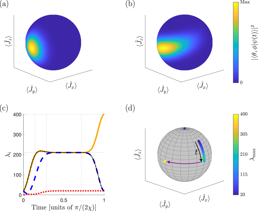
Figure 1: One-axis twisting with $N=20$. (a) and (b) Collective Bloch sphere at $t=0$ and $t=1/(\chi N^{\frac{2}{3}})$, respectively. The color represents $\absolutevalue{\innerproduct{\theta,\phi}{\psi(t)}}^{2}$ at each point. (c) The three eigenvalues $\lambda_{i}$ of $\bm{\mathcal{F}}$. Also plotted as a black dotted-dashed line is $\mathcal{F}_{\mathrm{OAT}}$ from Eq. (8). (d) Location of the optimal generator during the squeezing process. The color represents the QFI for the given generator. The time axis for $t\lesssim\pi/(2\chi)-2/(\chi\sqrt{N})$ is shown with a black arrow, while the discontinuous jump at $t\sim\pi/(2\chi)-2/(\chi\sqrt{N})$ is shown with a purple arrow. The eigenvalue then grows at this final axis for the remainder of the process.

We demonstrate squeezing of a CSS initially oriented along $\hat{J}_{x}=(\hat{u}^{\dagger}\hat{d}+\hat{d}^{\dagger}\hat{u})/2$, shown in Fig. 1(a), which reaches an optimally squeezed state at time $t=1/(\chi N^{\frac{2}{3}})$, shown in Fig. 1(b).

We now examine this well-known squeezing example through the lens of QFIM diagonalization. The operator basis of the $\mathrm{SU}(2)$ group is the collective operators $\hat{G}_{\mu}\in\{\hat{J}_{x},\hat{J}_{y},\hat{J}_{z}\}$, where $\hat{J}_{y}=i(\hat{d}^{\dagger}\hat{u}-\hat{u}^{\dagger}\hat{d})/2$. Therefore, Eq. (3) requires the diagonalization of a $3\times 3$ matrix $\bm{\mathcal{F}}$. Figure 1(c) shows the three eigenvalues of $\bm{\mathcal{F}}$ during the squeezing process. At $t=0$, the eigenvectors $\vec{Y}^{\mu}=(0,1,0)^{T}$ and $\vec{Z}^{\mu}=(0,0,1)^{T}$ have degenerate eigenvalues at the SQL, $\lambda_{\mathrm{max}}=N$. The third eigenvector $\vec{X}^{\mu}=(1,0,0)^{T}$ has a zero eigenvalue, showing the underlying symmetry of the initial CSS. The degenerate eigenvalues split as squeezing begins. As shown in Fig. 1(c), we find perfect agreement between the largest eigenvalue of $\bm{\mathcal{F}}$ and the analytical solution [11, 16] during the initial squeezing $t\lesssim 1/(\chi\sqrt{N})$,

$$\mathcal{F}_{\mathrm{OAT}}=N+\frac{N(N-1)}{4}\left(A+\sqrt{A^{2}+B^{2}}\right),$$ (8)

with $A=1-\cos^{N-2}(2\chi t)$ and $B=4\sin(\chi t)\cos^{N-2}(\chi t)$. We emphasize that this analytical result is found using the exact solution of the squeezing dynamics which allows one to extract the maximum QFI. Instead, with the help of the QFIM, we do not require any such insight into the state and yet can still efficiently find the maximum QFI numerically, deriving the eigenvector visible in Fig. 1(d) displaying the optimal generator $\hat{\mathcal{G}}$. However, we will see that the QFIM eigendecomposition offers its own insights into symmetries at points of a given system’s dynamics.

After $t=0$, the symmetry of the CSS is broken, and the optimal generator jumps to $\hat{\mathcal{G}}=\sin(\delta)\hat{J}_{z}+\cos(\delta)\hat{J}_{y}$, where we find perfect agreement with the expression $\delta=\arctan(B/A)/2$ given in Ref. [15]. As squeezing progresses, the optimal generator then rotates towards the equator. At $t\sim 2/(\chi\sqrt{N})$, the first two eigenvalues become degenerate with the associated eigenvectors $\vec{X}^{\mu}$ and $\vec{Y}^{\mu}$, once again showing an underlying symmetry of the state [17]. This symmetry is then broken at $t\sim\pi/(2\chi)-2/(\chi\sqrt{N})$, causing the two largest eigenvalues to split and a discontinuous jump of the optimal rotation axis from $\vec{Y}^{\mu}$ to $\vec{X}^{\mu}$ [purple arrow in Fig. 1(d)]. Therefore, Eq. (8) no longer calculates the maximum QFI because it corresponds to rotations about $\hat{J}_{y}$ when $t\gtrsim 2/(\chi\sqrt{N})$. We find that $\mathcal{F}_{\mathrm{OAT}}$ follows the second eigenvalue down to the SQL while the largest eigenvalue grows to the HL, $\lambda_{\mathrm{max}}=N^{2}$. The final three eigenvalues, one at HL and two at SQL, are only possible in $\mathrm{SU}(2)$ systems with a NOON state, which matches the analysis of Ref. [17]. Having demonstrated that the well-known results of OAT follow naturally from the diagonalization of the QFIM, we now turn to a higher dimensional system in which analytical results for the maximum QFI and optimal generator cannot readily be obtained.

Squeezing in higher dimensonal systems.— We consider a $N$-body system in which the constitute particles now have four states $\ket{u}$, $\ket{d}$, $\ket{s}$, and $\ket{c}$. We again utilize Schwinger bosons with corresponding creation operators $\hat{u}^{\dagger}$, $\hat{d}^{\dagger}$, $\hat{s}^{\dagger}$, and $\hat{c}^{\dagger}$. Here, the linear dynamics are described by the $\mathrm{SU}(4)$ group with six $\mathfrak{su}(2)$ sub-algebras. Each sub-algebra has the associated raising operators [54] $\hat{\mathcal{Q}}^{+}=\hat{u}^{\dagger}\hat{d}$, $\hat{\Sigma}^{+}=\hat{s}^{\dagger}\hat{c}$, $\hat{\mathcal{M}}^{+}=\hat{u}^{\dagger}\hat{c}$, $\hat{\mathcal{N}}^{+}=\hat{s}^{\dagger}\hat{d}$, $\hat{\mathcal{U}}^{+}=\hat{u}^{\dagger}\hat{s}$, and $\hat{\mathcal{V}}^{+}=\hat{c}^{\dagger}\hat{d}$. These operators define the Hermitian components of each algebra according to $\hat{O}_{x}=(\hat{O}^{+}+\hat{O}^{-})/2$, $\hat{O}_{y}=-i(\hat{O}^{+}-\hat{O}^{-})/2$, and $\hat{O}_{z}=[\hat{O}^{+},\hat{O}^{-}]/2$. We can then create an operator basis that spans $\mathfrak{su}(4)$ with 15 operators that satisfy the orthonormality property [48]:

$$\hat{G}_{\mu}\in\{ \hat{\mathcal{Q}}_{x},\hat{\mathcal{Q}}_{y},\hat{\mathcal{Q}}_{z},\hat{\Sigma}_{x},\hat{\Sigma}_{y},\hat{\Sigma}_{z},\hat{\mathcal{M}}_{x},\hat{\mathcal{M}}_{y},$$ (9)

$$\hat{\mathcal{N}}_{x},\hat{\mathcal{N}}_{y},\hat{\mathcal{P}}_{z},\hat{\mathcal{U}}_{x},\hat{\mathcal{U}}_{y},\hat{\mathcal{V}}_{x},\hat{\mathcal{V}}_{y}\},$$

where $\hat{\mathcal{P}}_{z}=(\hat{\mathcal{M}}_{z}-\hat{\mathcal{N}}_{z})/\sqrt{2}$.

We prepare the state via the nonlinear interaction

$$\hat{H}_{TAT}=\hbar\chi\left(\hat{\mathcal{Q}}^{+}+\hat{\Sigma}^{+}\right)\left(\hat{\mathcal{Q}}^{-}+\hat{\Sigma}^{-}\right)=2\hbar\chi\hat{E}^{+}\hat{E}^{-},$$ (10)

which causes twisting about three of the axes of a 15-dimensional collective hypersphere [27]. Here, we have introduced three $\mathrm{SU}(2)$ subgroups $\mathfrak{J}$, $\mathfrak{K}$, and $\mathfrak{E}$ generated by algebras with raising operators $\hat{J}^{+}=(\hat{\mathcal{M}}^{+}+\hat{\mathcal{N}}^{+})/\sqrt{2}$, $\hat{K}^{+}=(\hat{\mathcal{U}}^{+}+\hat{\mathcal{V}}^{+})/\sqrt{2}$, and $\hat{E}^{+}=(\hat{\mathcal{Q}}^{+}+\hat{\Sigma}^{+})/\sqrt{2}$, respectively. The $\mathfrak{J}$ and $\mathfrak{K}$ algebras might represent the dynamics of the internal and external degrees of freedom of atoms in a dispersive Kapitza-Dirac cavity, while the $\mathfrak{E}$ algebras represents the entanglement-generating processes [27, 48].

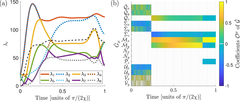
Figure 2: Three-axis twisting of a $\mathrm{SU}(4)$ system with $N=20$. (a) The largest eight eigenvalues $\lambda_{i}$ of $\bm{\mathcal{F}}$. Also shown as a black dashed line is the largest QFI from an operator in the $\mathfrak{J}$, $\mathfrak{K}$, and $\mathfrak{E}$ subgroups. (b) Coefficients $\mathcal{O}^{\mu}$ and corresponding basis operator $\hat{G}_{\mu}$ of the optimal generator $\hat{\mathcal{G}}=\mathcal{O}^{\mu}\hat{G}_{\mu}$.

When we begin in a simultaneous eigenstate of $\hat{J}_{x}$ and $\hat{K}_{y}$, $\ket{\psi_{0}}=(N!)^{-\frac{1}{2}}\exp[-i\hat{J}_{y}\pi/\sqrt{2}](\hat{u}^{\dagger})^{N}\ket{0}$, the Hamiltonian Eq. (10) causes squeezing as well as non-trivial entanglement between $\mathfrak{J}$ and $\mathfrak{K}$. We display the dynamics of the QFIM eigenvalues for $N=20$ in Fig. 2(a) and the eigenvector of the QFIM with the largest eigenvalue in Fig. 2(b). Figure 2(a) also displays the maximum QFI from operators in the $\mathfrak{J}$, $\mathfrak{K}$, and $\mathfrak{E}$ subgroups, which were the generators considered in Ref. [27]. At $t=0$, the largest six eigenvalues are degenerate at the SQL, $\lambda_{i}=N$, indicating that the starting state is a generalized CSS [55]. This mirrors the symmetry between $\vec{Y}^{\mu}$ and $\vec{Z}^{\mu}$ initially in OAT, but now over three $\mathrm{SU}(2)$ subgroups [56]. As the squeezing begins, the largest two eigenvalues grow until $t\sim 1/(\chi\sqrt{N})$ where they reach a maximum value of $\lambda_{\mathrm{max}}\sim 146\approx 0.366N^{2}$. This degeneracy can be seen in Fig. 2(b) as the optimal generator jumps back and forth between two operators for the beginning of the squeezing process. These two degenerate eigenvalues subsequently fall until they cross the third largest eigenvalue at $t\sim 5/(3\chi\sqrt{N})$, corresponding to a discontinuous jump in Fig. 2(b). The eigenvalue corresponding to a rotation axis close to $\hat{\mathcal{M}}_{x}$ then grows rapidly, eventually becoming the largest eigenvalue at $t\sim\pi/(2\chi)-1/(\chi\sqrt{N})$. This analysis highlights that the QFIM diagonalization unravels the complicated nonlinear dynamics of the high dimensional quantum system. In fact, with its help, we find that at all times the state has a higher sensitivity than what was shown in Ref. [27].

Multiparameter estimation.— So far, we have focused on optimizing single parameter estimation. However, our QFIM diagonalization scheme inherently optimizes multiparameter estimation as well by finding multiple eigenvectors of the QFIM whose complimentary generators commute with one another. This, in turn, could be used in quantum sensors that aim to infer multiple parameters beyond the SQL simultaneously. As an example, at $t=\pi/(4\chi)$ in Fig. 2(a), the generators associated with the eigenvalues $\lambda_{1}=0.307\,N^{2}$, $\lambda_{3}=0.189\,N^{2}$, and $\lambda_{8}=0.117\,N^{2}$ all commute with one another, meaning one could carry out simultaneous estimation beyond the SQL for all three of the corresponding parameters. The associated generators go as $\hat{\mathcal{G}}_{1}=c_{1}\sqrt{2}\hat{K}_{z}+c_{2}(\hat{\mathcal{M}}_{x}+\hat{\mathcal{M}}_{y})$, $\hat{\mathcal{G}}_{3}=c_{2}\sqrt{2}\hat{K}_{z}-c_{1}(\hat{\mathcal{M}}_{x}+\hat{\mathcal{M}}_{y})$, and $\hat{\mathcal{G}}_{8}=c_{3}\hat{\mathcal{N}}_{x}+c_{4}\hat{\mathcal{N}}_{y}$, with real coefficients $c_{i}$ that satisfy the normalization condition. For the case of the spin-momentum $\textrm{SU}(4)$ system considered in Ref. [27], a portion of these generators may be found to correspond to interactions which are more physically accessible than the whole generator is [see SM [48] for details]. In this physical example, $\hat{K}_{z}$ could correspond to a linear acceleration while $\hat{\mathcal{M}}_{x}+\hat{\mathcal{M}}_{y}$ and $c_{3}\hat{\mathcal{N}}_{x}+c_{4}\hat{\mathcal{N}}_{y}$ may correspond to spatially dependent rotations, thereby creating the opportunity for many combinations of useful interferometry [37, 57, 58]. We thus consider $(\hat{\mathcal{M}}_{x}+\hat{\mathcal{M}}_{y})/\sqrt{2}$, $\hat{K}_{z}$, and $\hat{\mathcal{G}}_{8}$ which still have QFIs of $0.300\,N^{2}$, $0.195\,N^{2}$, and $0.117\,N^{2}$, respectively. Since these operators are in three commuting sub-algebras, they can be independently rotated to any arbitrary operator in the respective sub-algebra in order to be made relevant for sensing vector quantities or network node interferometry [58, 59, 60].

More generally, within $\mathrm{SU}(n)$, one is guaranteed sets of $n-1$ commuting generators [48, 61, 62], thereby guaranteeing sets of $n-1$ eigenvectors of the QFIM which correspond to simultaneously commuting generators. One could thus select the eigenvector with the largest eigenvalue and search the remaining eigenvectors to find the set of $n-1$ generators which mutually commute and have suitable eigenvalues that scale beyond the SQL. Furthermore, the associated symmetric logarithmic derivatives $\hat{L}_{\mu}$ are guaranteed to commute such that the optimal measurement basis is the same for each parameter. This ensures that the QCRB is always simultaneously attainable for all $n-1$ parameters as the elements of the Uhlmann curvature matrix $\mathbb{U}_{\mu\nu}=-i\Tr[\rho[\hat{L}_{\mu},\hat{L}_{\nu}]]/2$ will vanish [28, 63, 64, 65].

Conclusion and outlook.— We have demonstrated that the optimal generator for quantum sensing is given by the eigenvector associated with the largest eigenvalue of the QFIM. This is a consequence of maximizing differential path lengths through quantum state space when the QFIM is viewed as a Riemannian metric, generalizing the work of Ref. [66] to any metrological process with an underlying Lie group structure. For the examples we considered, unitary parameterization was assumed, but future steps include examining a channel or hybrid parameterization scheme [28, 67, 68] using QFIM diagonalization. Furthermore, our examples have used pure states, but the procedure is equally valid with mixed states and the properly defined tangent vectors. Here, one must utilize the more general definition of the QFIM given in Ref. [28]. The use of mixed states is then relevant to experiments where a small amount of entanglement entropy between the system and a bath can be generated through either known or unknown dissipative processes.

The examples we considered had underlying $\mathrm{SU}(2)$ and $\mathrm{SU}(4)$ group dynamics. Already in the case of $\mathrm{SU}(4)$, one finds that more care must be taken compared to the $\mathrm{SU}(2)$ case when considering larger group structures. For one, unitarily rotating the optimal generator to an arbitrary operator is not always possible in larger group structures [48]. We also outline in the SM [48] how to extend our work to general $\mathrm{SU}(n)$ systems with an algorithm to generate an orthogonal operator basis that spans the quantum state space. Moreover, the underlying formalism of this Letter extends to any dynamical group structure. This makes our procedure relevant to systems described by $\mathrm{Sp}(n,\mathbb{R})$ [69, 70], $\mathrm{SU}(m,n)$ [71], or translational groups [72], for example.

Interestingly, there have been recent efforts to experimentally infer the quantum geometric tensor [73, 74, 75, 76], which is related to the QFI metric through its real component [48, 51]. This leads to the prospect of finding the optimal generator for quantum sensing without the need for a full theoretical model, only an understanding of the underlying symmetries. This is necessary for complex systems where such models are difficult to derive or fully simulate. Our QFIM diagonalization procedure thus opens an exciting avenue for experiments with complex systems [25, 77, 78, 79, 80, 81, 24, 26, 82], whose current interest is not parameter estimation, to naturally test if the experiment can be useful as a quantum sensor and how to use any generated entanglement in an efficient manner. In addition, we can combine numerical approaches with QFIM diagonalization for these complex systems, which is relevant for quantum optical control and machine learning methods that have been used effectively for quantum design tasks [83, 84, 85, 86, 87, 88, 89].