Nonsmooth optimality criterion for a $\mathrm{W}^{1,2}$-controlled sweeping process: Nonautonomous perturbation

¹Department of Computer Science and Mathematics, Lebanese American University, Byblos Campus,
P.O. Box 36, Byblos, Lebanon
²Department of Mathematics, Michigan State University, East Lansing, MI 48824-1027, USA

Abstract. We extend to $\mathrm{C}\scaleto{\times}{6pt}\mathrm{W}^{1,2}$-local minimizers and nonautonomous perturbation function, the necessary optimality conditions derived in [1], via continuous-time approximations, for $\mathrm{W}^{1,2}\scaleto{\times}{6pt}\mathrm{W}^{1,2}$-local minimizers of an optimal control problem governed by a controlled nonconvex sweeping process with autonomous perturbation function.
Keywords. Controlled and perturbed nonconvex sweeping process; Local minimizers; Necessary optimality conditions; Continuous-time approximations; Nonsmooth analysis.

1. Introduction

Moreau’s sweeping process is a mathematical model introduced in [2, 3, 4] to describe an elastoplastic mechanical system. Since then, this model appeared in several fields such as mechanics, electrical circuits, engineering, economics, crowd motion control, traffic equilibria, hysteresis phenomena, etc. (see, e.g., [5] and its references). Since the dynamic of this model is an evolution differential inclusions involving an unbounded and discontinuous multifunction, namely, the normal cone to a set, the sweeping process model falls outside the scope of standard differential inclusions. Therefore, new techniques are required to address optimal control problems over sweeping processes.

In this paper, we are interested in deriving necessary optimality conditions, phrased in terms of the weak-Pontryagin-type maximum principle, for optimal control problems governed by $\mathrm{W}^{1,2}$-controlled and nonautonomously perturbed sweeping processes. The autonomous case was successfully treated in [6, 7, 8] via discrete approximations, and in [1] via continuous approximations. In these references, the authors considered $\mathrm{W}^{1,2}\scaleto{\times}{6pt}\mathrm{W}^{1,2}$-local minimizers, and obtained in addition to necessary optimality conditions, the strong convergence of velocities, that is, the optimal states of the original problem are strongly approximated, in the $\mathrm{W}^{1,2}$-norm, by the optimal states of the approximating problems. It is worth to mention that, unlike the case for standard optimal control problems where the optimal control functions have weak regularity properties, applications of optimal control problems over sweeping processes have shown to possess optimal control functions having strong regularity properties, such as, $\mathrm{W}^{1,2}$ (see e.g., [7], [8, Examples 9.1 & 9.2]).

The continuous approximation used in [1] is based on approximating the normal cone by an exponential penalization term. This innovative technique was introduced in [9, 10], and further developed in [11, 12, 13, 14, 15]. The autonomous assumption on the perturbation function in [1], and also in [6, 7, 8], played a crucial role in the derivation of the necessary optimality conditions using $W^{1,2}$-controls, especially, in the proof of the strong convergence of velocities.

The goal of this paper is to extend the weak Pontryagin maximum principle derived in [1] to the case where the perturbation function is nonautonomous and the $t$-dependence is merely measurable. In order to reach this goal, it turns out that the strong convergence of velocities has to be weakened in the following sense: While the convergence of the approximating problems solutions to those of the original problem remains uniform for the state component and strong in $\mathrm{W}^{1,2}$ for the control component, it is rather weak* in $L^{\infty}$ for the state velocities. Consequently, our necessary optimality conditions, which coincide with those obtained in [1], are derived for $\mathrm{C}\scaleto{\times}{6pt}\mathrm{W}^{1,2}$-local minimizers. For this class of local minimizers, our formulation here of the approximating problems via the exponential penalization technique is different than that in [1], and so is the proof of existence of optimal solutions for these problems (Lemma 3.1) as well as the proof of Lemma 3.2.

The paper is organized as follows. In the next section, we present our basic notations, we define our optimal control problem $(P)$ governed by a $\mathrm{W}^{1,2}$-controlled and perturbed sweeping process, we list the hypotheses satisfied by the data of $(P)$, and we state the main result of the paper, namely, necessary optimality conditions in the form of weak Pontryagin principle for $\mathrm{C}\scaleto{\times}{6pt}\mathrm{W}^{1,2}$-local minimizers of $(P)$. Section 3 is devoted to the proof of our main result. An example illustrating the utility of our main result is provided in Section 4.

2. Main result

2.1. Basic notations

The following are the basic notations and definitions used in this paper:

• For the Euclidean norm and the usual inner product, we use $\|\cdot\|$ and $\langle\cdot,\cdot\rangle$, respectively.

• For $y\in\mathbb{R}^{n}$ and $r>0$, we define the open (resp. closed) ball centered at $y$ with radius $r$ as $B_{r}(y):=y+rB$ (resp. $\bar{B}_{r}(y):=y+r\bar{B}$), where $B$ and $\bar{B}$ denotes the open and the closed unit ball, respectively.

• For $C\subset\mathbb{R}^{n}$, the boundary, the interior, the closure, the convex hull, the complement, and the polar of $C$ are denoted by $\textnormal{bdry}\,C$, $\textnormal{int}\,C$, $\textnormal{cl}\,C$, $\textnormal{conv}\,C$, $C^{c}$, and $C^{\circ}$, respectively.

• The distance from a point $x\in\mathbb{R}^{n}$ to a set $C\subset\mathbb{R}^{n}$ is denoted by $d(x,C)$.

• For an extended-real-valued function $h\colon\mathbb{R}^{n}\longrightarrow\mathbb{R}\cup\{\infty\}$, the effective domain of $h$ is $\textnormal{dom}\,h$, and the epigraph of $h$ is $\textnormal{epi}\,h$.

• For a multifunction $F\colon\mathbb{R}^{n}\rightrightarrows\mathbb{R}^{m}$, we denote by $\textnormal{Gr}\,F\subset\mathbb{R}^{n}\times\mathbb{R}^{m}$ the graph of $F$.

• The space $L^{p}([a,b];\mathbb{R}^{n})$ designates the Lebesgue space of $p$-integrable functions $h\colon[a,b]\longrightarrow\mathbb{R}^{n}$. We denote by $\|\cdot\|_{p}$ and $\|\cdot\|_{\infty}$ the norms of $L^{p}([a,b];\mathbb{R}^{n})$ and $L^{\infty}([a,b];\mathbb{R}^{n})$ (or $\mathrm{C}([a,b];\mathbb{R}^{n})$), respectively. For $C\subset\mathbb{R}^{d}$ compact, the set of continuous functions from $C$ to $\mathbb{R}^{n}$ is denoted by $\mathrm{C}(C;\mathbb{R}^{n})$.

• The set of all $m\times n$-matrix functions on $[a,b]$ is denoted by $\mathscr{M}_{m\times n}([a,b])$.

• A function $h\colon[a,b]\longrightarrow\mathbb{R}^{n}$ is said to be a $BV$-function if $h$ has a bounded variation. The set of all such functions is denoted by $BV([a,b];\mathbb{R}^{n})$. We denote by $NBV[a,b]$ the normalized space of $BV$-functions on $[a,b]$ that consists of those $BV$-functions $h$ such that $h(a)=0$ and $h$ is right continuous on $(a,b)$ (see e.g., [16, p.115]).

• The space $\mathrm{C}^{*}([a,b];\mathbb{R})$ denotes the dual of $\mathrm{C}([a,b];\mathbb{R}),$ equipped with the supremum norm. The induced norm on $\mathrm{C}^{*}([a,b];\mathbb{R})$ is denoted by $\|\cdot\|_{\textnormal{\tiny{T.\hskip 0.42677ptV.}}}$. As a consequence of Riesz representation theorem, we can interpret the elements of $\mathrm{C}^{*}([a,b];\mathbb{R})$ as being in $\mathfrak{M}([a,b])$, the set of finite signed Radon measures on $[a,b]$ equipped with the weak* topology. Thereby, to each element of $\mathrm{C}^{*}([a,b];\mathbb{R})$ it corresponds a unique element in $NBV[a,b]$ related through the Stieltjes integral and both elements have the same total variation. The set $\mathrm{C}^{\oplus}(a,b)$ designates the subset of $\mathrm{C}^{*}([a,b];\mathbb{R})$ taking nonnegative values on nonnegative-valued functions in $\mathrm{C}([a,b];\mathbb{R})$.

• By $\mathrm{W}^{k,p}([a,b];\mathbb{R}^{n})$, $k\in\mathbb{N}$ and $p\in[0,+\infty]$, we denote the classical Sobolev space. Hence, the set of all absolutely continuous functions from $[a,b]$ to $\mathbb{R}^{n}$ is $\mathrm{W}^{1,1}([a,b];\mathbb{R}^{n})$. Note that in this paper, the Sobolev space $\mathrm{W}^{1,2}([a,b];\mathbb{R}^{m})$ will be considered with the norm $\|u(\cdot)\|_{W^{1,2}}:=\|u(\cdot)\|_{\infty}+\|\dot{u}(\cdot)\|_{2}.$ Hence, the convergence of a sequence $u_{n}$ strongly in the norm topology of the space $W^{1,2}([a,b];\mathbb{R}^{m})$ is equivalent to the uniform convergence of $u_{n}$ on $[a,b]$ and the strong convergence in $L^{2}$ of its derivative $\dot{u}_{n}$.

• For $C\subset\mathbb{R}^{n}$ closed and $c\in C$, we denote by $N^{P}_{C}(c)$, $N_{C}^{L}(c)$, and $N_{C}(c)$, the proximal, the Mordukhovich (or limiting), and the Clarke normal cones to $C$ at $c$, respectively.

• For $F\colon[a,b]\rightrightarrows\mathbb{R}^{m}$ a multifunction with closed and nonempty values, $\bar{N}^{L}_{F(t)}(y)$ stands for the graphical closure at $(t,y)$ of the multifunction $(t,y)\mapsto{N}^{L}_{F(t)}(y)$, that is, the graph of $\bar{N}^{L}_{F(\cdot)}(\cdot)$ is the closure of the graph of $N^{L}_{F(\cdot)}(\cdot)$.

• For $h\colon\mathbb{R}^{n}\longrightarrow\mathbb{R}\cup\{\infty\}$ lower semicontinuous and $x\in\textnormal{dom}\,h$, we denote by $\partial^{P}h(x)$, $\partial^{L}h(x)$, and $\partial h(x)$ the proximal, the Mordukhovich (or limiting), and the Clarke subdifferential of $h$ at $x$, respectively. Note that if $h$ is Lipschitz near $x$, then the Clarke generalized gradient of $h$ at $x$ is also denoted by $\partial h(x)$.

• If $h\colon\mathbb{R}^{n}\longrightarrow\mathbb{R}\cup\{\infty\}$ is $\mathsf{C}^{1,1}$ near $x\in\textnormal{dom}\,h$, then the Clarke generalized Hessian of $h$ at $x$ is denoted by $\partial^{2}h(x)$. On the other hand, if $H\colon\mathbb{R}^{n}\longrightarrow\mathbb{R}^{n}$ is Lipschitz near $x\in\mathbb{R}^{n}$, then the Clarke generalized Jacobian of $H$ at $x$ is denoted by $\partial{H}(x)$.

• For $F\colon[a,b]\rightrightarrows\mathbb{R}^{m}$ a lower semicontinuous multifunction with closed and nonempty values, we define

  $$\hskip 36.98866pt\partial_{x}^{\hskip 0.42677pt>}d(x,F(t)):=\textnormal{conv}\,\left\{\zeta=\lim_{i\longrightarrow\infty}\zeta_{i}:\;\|\zeta_{i}\|=1,\;\zeta_{i}\in N_{F(t_{i})}^{P}(x_{i})\;\hbox{and}\;(t_{i},x_{i})\xrightarrow{{\textnormal{Gr}\,F}}(t,x)\right\},$$

  where $(t_{i},x_{i})\xrightarrow{{\textnormal{Gr}\,F}}(t,x)$ signifies that $(t_{i},x_{i})\longrightarrow(t,x)$ with $x_{i}\in F(t_{i})$ for all $i$. Note that $\partial_{x}^{\hskip 0.42677pt>}d(x,F(t))$ coincides with $\partial_{x}^{\hskip 0.42677pt>}g(t,x)$ of [17, p.121] for $g(t,x):=d(x,F(t))$, see [18, Corollary 2.2].

• For $r>0$, a closed and nonempty set $S\subset\mathbb{R}^{n}$ is said to be $r$-prox-regular if for all $s\in\textnormal{bdry}\,S$ and for all $\zeta\in N_{S}^{P}(s)$ unit, we have $\langle\zeta,x-s\rangle\leq\frac{1}{2r}\|x-s\|^{2}$ for all $x\in S.$ For more information about prox-regularity, see [19].

2.2. Statement of the problem $(P)$ and hypotheses

We consider the following fixed time Mayer-type optimal control problem involving $\mathrm{W}^{1,2}$-controlled and perturbed sweeping systems

$$\begin{array}[]{l}(P)\colon\;\hbox{Minimize}\;g(x(0),x(1))\vspace{0.1cm}\\ \hskip 25.6073pt\hbox{over}\;(x,u)\in\mathrm{W}^{1,1}([0,1];\mathbb{R}^{n})\times\mathscr{W}\;\hbox{such that}\\[2.0pt] \hskip 25.6073pt\begin{cases}(D)\left[\begin{array}[]{@{}l@{\quad}l@{}}\dot{x}(t)\in f(t,x(t),u(t))-\partial\varphi(x(t)),\;\;\hbox{a.e.}\;t\in[0,1],\\ x(0)\in C_{0}\subset\textnormal{dom}\,\varphi,\end{array}\right.\vspace{0.1cm}\\ x(1)\in C_{1},\end{cases}\end{array}$$

where, $g\colon\mathbb{R}^{n}\times\mathbb{R}^{n}\longrightarrow\mathbb{R}\cup\{\infty\}$, $f\colon[0,1]\times\mathbb{R}^{n}\times\mathbb{R}^{m}\longrightarrow\mathbb{R}^{n}$, $\varphi\colon\mathbb{R}^{n}\longrightarrow\mathbb{R}\cup\{\infty\}$, $\partial$ stands for the Clarke subdifferential, $C:=\textnormal{dom}\,\varphi$ is the zero-sublevel set of a function $\psi\colon\mathbb{R}^{n}\longrightarrow\mathbb{R}$, that is, $C=\{x\in\mathbb{R}^{n}:\psi(x)\leq 0\},$ $C_{0}\subset C$, $C_{1}\subset\mathbb{R}^{n}$, and, for $U\colon[0,1]\rightrightarrows\mathbb{R}^{m}$ a multifunction and $\mathbb{U}:=\bigcup_{t\in[0,1]}U(t)$, the set of control functions $\mathscr{W}$ is defined by

$$\mathscr{W}:=\mathrm{W}^{1,2}([0,1];\mathbb{U})=\left\{u\in\mathrm{W}^{1,2}([0,1];\mathbb{R}^{m}):u(t)\in U(t),\;\;\forall\hskip 0.42677ptt\in[0,1]\right\}.$$

Note that if $(x,u)$ solves ($D$), it necessarily follows that $x(t)\in C$, $\forall\hskip 0.42677ptt\in[0,1]$.

A pair $(x,u)$ is admissible for $(P)$ if $x\colon[0,1]\longrightarrow\mathbb{R}^{n}$ is absolutely continuous, $u\in\mathscr{W}$, and $(x,u)$ satisfies the controlled  and perturbed sweeping process $(D)$, called the dynamic of $(P)$. An admissible pair $(\bar{x},\bar{u})$ for $(P)$ is said to be a $\mathrm{C}\scaleto{\times}{6pt}\mathrm{W}^{1,2}$-local minimizer if there exists $\delta>0$ such that

$$g(\bar{x}(0),\bar{x}(1))\leq g(x(0),x(1)),$$ (2.1)

for all $(x,u)$ admissible for $(P)$ with $\|x-\bar{x}\|_{\infty}\leq\delta$, $\|u-\bar{u}\|_{\infty}\leq\delta$ and $\|\dot{u}-\dot{\bar{u}}\|_{2}^{2}\leq\delta$. Note that if the inequality (2.1) is satisfied by any admissible pairs $(x,u)$, then $(\bar{x},\bar{u})$ is called a global minimizer (or an optimal solution ) for $(P)$.

Let $(\bar{x},\bar{u})$ be a $\mathrm{C}\scaleto{\times}{6pt}\mathrm{W}^{1,2}$-local minimizer for $(P)$ with associated $\delta$, such that the following hypotheses hold for $\bar{\mathbb{B}}_{\delta}(\bar{x}):=\bigcup\limits_{t\in[0,1]}\bar{B}_{\delta}(\bar{x}(t))$:

1. There exist $\tilde{\rho}>0$ and $M_{\ell}>0$ such that $f(\cdot,x,u)$ is Lebesgue-measurable for $(x,u)\in[C\cap\bar{\mathbb{B}}_{\delta}(\bar{x})]\times[(\mathbb{U}+\tilde{\rho}\bar{B})\cap\bar{\mathbb{B}}_{\delta}(\bar{u})]$; and for a.e. $t\in[0,1]$ we have: $(x,u)\mapsto f(t,x,u)$ is $M_{\ell}$-Lipschitz on $\left[C\cap\bar{B}_{\delta}(\bar{x}(t))\right]\times\left[\big{(}U(t)+\tilde{\rho}\bar{B}\big{)}\cap\bar{B}_{\delta}(\bar{u}(t))\right]$; and $\|f(t,x,u)\|\leq M_{\ell}$ for all $(x,u)\in\left[C\cap\bar{B}_{\delta}(\bar{x}(t))\right]\times\left[U(t)\cap\bar{B}_{\delta}(\bar{u}(t))\right].$

2. The set $C:=\textnormal{dom}\,\varphi$ is given by $C=\{x\in\mathbb{R}^{n}:\psi(x)\leq 0\},$ where $\psi:\mathbb{R}^{n}\longrightarrow\mathbb{R}.$

   1. There exists $\rho>0$ such that $\psi$ is $\mathsf{C}^{1,1}$ on $C+\rho{B}$.

   2. There is a constant $\eta>0$ such that $\|\nabla\psi(x)\|>2\eta\;$ for all $x$ satisfying $\psi(x)=0.$

   3. The function $\psi$ is coercive, that is, $\lim_{\|x\|\longrightarrow\infty}\psi(x)=+\infty.$

   4. The set $C$ has a connected interior.

3. The function $\varphi$ is globally Lipschitz on $C$ and $\mathsf{C}^{1}$ on $\textnormal{int}\,C$. Moreover, the function $\nabla\varphi$ is globally Lipchitz on $\textnormal{int}\,C$.

4. For the sets $C_{0}$, $C_{1}$, and $U(\cdot)$ we have:

   1. The set $C_{0}\subset C$ is nonempty and closed.

   2. The graph of $U(\cdot)$ is a $\mathscr{L}\times\mathscr{B}$ measurable set, and, for $t\in[0,1],$ $U(t)$ is closed, and bounded uniformly in $t$.

   3. The set $C_{1}\subset\mathbb{R}^{n}$ is nonempty and closed.

   4. The multifunction $U(\cdot)$ is lower semicontinuous.

   5. The multifunction $U(\cdot)$ satisfies the constraint qualification (CQ) at $\bar{u}$, that is,

      $$\textnormal{conv}\,(\bar{N}^{L}_{U(t)}(\bar{u}(t)))\;\hbox{is pointed}\;\,\forall t\in[0,1].$$

5. There exist $\tilde{\rho}>0$ and $L_{g}>0$ such that $g$ is $L_{g}$-Lipschitz on $\tilde{C}_{0}(\delta)\times\tilde{C_{1}}(\delta)$, where

   $$\tilde{C}_{i}(\delta):=\big{[}\left(C_{i}\cap\bar{B}_{\delta}(\bar{x}(i))\right)+\tilde{\rho}\bar{B}\big{]}\cap C,\;\;\text{for}\;\;i=0,1.$$

Let $M_{C}$ be a bound of the compact set $C$. We denote by $\bar{M}_{\psi}$ an upper bound of $\|\nabla\psi(\cdot)\|$ on $C$, and by $2M_{\psi}$ a Lipschitz constant of $\nabla\psi(\cdot)$ over the compact set $C+\frac{\rho}{2}\bar{B}$ chosen large enough so that $M_{\psi}\geq\frac{4\eta}{\rho}.$

Remark 2.1.

Since $f$ satisfies (H1), then by [20, Theorem 1] applied to each component, $f_{i}$, of $f=(f_{1},\cdots,f_{n})$, there exists a function $\tilde{f}\colon[0,1]\times\mathbb{R}^{n}\times\mathbb{R}^{m}\longrightarrow\mathbb{R}^{n}$, such that, for almost all $t\in[0,1]$, $\tilde{f}(t,\cdot,\cdot)$ is globally Lipschitz on $\mathbb{R}^{n}\times\mathbb{R}^{m}$, and $f(t,x,u)=\tilde{f}(t,x,u)$ for all $(x,u)\in\left[C\cap\bar{B}_{\delta}(\bar{x}(t))\right]\times\left[\big{(}U(t)+\tilde{\rho}\bar{B}\big{)}\cap\bar{B}_{\delta}(\bar{u}(t))\right]$. Moreover, there exists a new constant $M\geq M_{\ell}$ such that $\tilde{f}$ satisfies the assumption (A1) of [14], in which the constant multifunction $U$ is replaced by $U(\cdot)\cap\bar{B}_{\delta}(\bar{u}(\cdot))$. Since in this paper we only consider local optimality notions, then, without loss of generality, we shall use the function $f$ instead of its extension $\tilde{f}$. In particular, we use that $f$ satisfies the assumption (A1) of [14], and hence, all the results of [14, Sections 3, 4 & 5] are valid. Now, by [14, Lemma 3.4], $C$ is $\frac{\eta}{M_{\psi}}$-prox-regular, and $\varphi$ admits a $\mathsf{C}^{1}$-extension $\varPhi$ from $C$ to $\mathbb{R}^{n}$ satisfying $\partial\varphi(x)=\{\nabla\varPhi(x)\}+N_{C}(x)$ for all $x\in C$, with

$$N_{C}(x)=\{\lambda\nabla\psi(x):\lambda\geq 0\},\;\forall x\in\textnormal{bdry}\,C,$$ (2.2)

and for some $K>0$,

$$\lvert\varPhi(x)\rvert\leq K\;\,\hbox{and}\;\,\|\nabla\varPhi(x)\|\leq K,\;\,\forall x\in\mathbb{R}^{n},\;\,\hbox{and}\;\,\|\nabla\varPhi(x)-\nabla\varPhi(y)\|\leq K\|x-y\|,\;\,\forall x,\,y\in\mathbb{R}^{n}.$$

This gives that $(D)$ can be equivalently phrased in terms of the normal cone to $C$ and the extension $\varPhi$ of $\varphi$, as follows

$$(D)\left[\begin{array}[]{@{}l@{\quad}l@{}}\dot{x}(t)\in f_{\varPhi}(t,x(t),u(t))-N_{C}(x(t)),\;\;\hbox{a.e.}\;t\in[0,1],\\ x(0)\in C_{0}\subset C,\end{array}\right.\\$$

where $f_{\varPhi}\colon[0,1]\times\mathbb{R}^{n}\times\mathbb{R}^{m}\longrightarrow\mathbb{R}^{n}$ is defined by

$$f_{\varPhi}(t,x,u):=f(t,x,u)-\nabla\varPhi(x),\;\;\;\forall(t,x,u)\in[0,1]\times\mathbb{R}^{n}\times\mathbb{R}^{m},$$

and hence, $\|f_{\varPhi}(t,x,u)\|\leq\bar{M}:=M+K$.

The following notations and facts, extracted from [14], will be used throughout the paper.

• For any $(x,u)$ solution of $(D)$, we have by [14, Equation 50] that

  $$\|\dot{x}(t)-f_{\varPhi}(t,x(t),u(t))\|\leq\|f_{\varPhi}(t,x(t),u(t))\|\leq\bar{M},\;\;t\in[0,1]\;\text{a.e.,}$$

  and hence, $\|\dot{x}\|_{\infty}\leq 2\bar{M}$.

• For given $x(\cdot)\colon[0,1]\to\mathbb{R}^{n},$ we define

  $$I^{0}(x):=\{t\in[0,1]:x(t)\in\textnormal{bdry}\,C\}\;\,\hbox{and}\;\,I^{\textnormal{-}}(x):=[0,1]\setminus I^{0}(x).$$

• We define the set $\mathscr{U}$ by

  $$\mathscr{U}:=\{u:[0,1]\to\mathbb{R}^{m}:u\;\hbox{is measurable and}\;u(t)\in U(t),\;t\in[0,1]\;\hbox{a.e.}\}.$$

• For $(x,u)\in\mathrm{W}^{1,1}([0,1];\mathbb{R}^{n})\times\mathscr{U}$ with $x(0)\in C_{0}$ and $x(t)\in C$ for all $t\in[0,1]$, we have from (2.2) and Filippov selection theorem ([21, Theorem 2.3.13]) that $x$ is a solution for $(D)$ corresponding to the control $u$ if and only if there exists a nonnegative measurable function $\xi$ supported on $I^{0}(x)$ such that $(x,u,\xi)$ satisfies

  $$\dot{x}(t)=f_{\varPhi}(t,x(t),u(t))-\xi(t)\nabla\psi(x(t)),\;\;\;t\in[0,1]\;\textnormal{a.e.}$$ (2.3)

  In this case, the nonnegative function $\xi$ supported in $I^{0}(x)$ with $(x,u,\xi)$ satisfying equation (2.3), is unique, belongs to $L^{\infty}([0,1];\mathbb{R}^{+})$, and

  $$\begin{cases}\xi(t)=0&\;\;\hbox{for}\;\;t\in I^{\textnormal{-}}(x),\\[4.0pt] \xi(t)=\frac{\|\dot{x}(t)-f_{\varPhi}(t,x(t),u(t))\|}{\|\nabla\psi(x(t))\|}\in\left[0,\frac{\bar{M}}{2\eta}\right]&\;\;\hbox{for}\;\;t\in I^{0}(x)\;\textnormal{a.e.},\\[5.0pt] \|\xi\|_{\infty}\leq\frac{\bar{M}}{2\eta}.\end{cases}$$ (2.4)

• Since $(\bar{x},\bar{u})$ solves the dynamic $(D)$, we denote by $\bar{\xi}$ the corresponding function in $L^{\infty}([0,1];\mathbb{R}^{+})$ such that $(\bar{x},\bar{u},\bar{\xi})$ satisfies (2.3) and (2.4).

• Let $(\gamma_{k})_{k}$ be a sequence satisfying

  $$\gamma_{k}>\frac{2\bar{M}}{\eta}\;\,\hbox{for all}\;k\in\mathbb{N},\;\hbox{and}\;\gamma_{k}\xrightarrow[k\longrightarrow\infty]{}\infty.$$ (2.5)

• The sequence $(\alpha_{k})_{k}$ is defined by

  $$\alpha_{k}:=\frac{\ln\left(\frac{\eta\gamma_{k}}{2\bar{M}}\right)}{\gamma_{k}},\;\;\;k\in\mathbb{N}.$$ (2.6)

  By (2.5) and (2.6), we have that

  $$\gamma_{k}e^{-\alpha_{k}\gamma_{k}}=\frac{2\bar{M}}{\eta},\;\;\alpha_{k}>0,\;\;\alpha_{k}\searrow\;\hbox{and}\;\lim_{k\longrightarrow\infty}\alpha_{k}=0.$$ (2.7)

• The sequence $(\rho_{k})_{k}$ is defined by $\rho_{k}:=\frac{\alpha_{k}}{\eta}$ for all $k\in\mathbb{N}$. By (2.7) we have that $\rho_{k}>0$ for all $k\in\mathbb{N}$, $\rho_{k}\searrow\,$ and $\,\lim\limits_{k\longrightarrow\infty}\rho_{k}=0.$

• For $k\in\mathbb{N}$, the approximating system $(D_{\gamma_{k}})$ is defined as

  $$({D}_{\gamma_{k}})\left[\begin{array}[]{@{}l@{\quad}l@{}}\dot{x}(t)=f_{\varPhi}(t,x(t),u(t))-\gamma_{k}e^{\gamma_{k}\psi(x(t))}\nabla\psi(x(t))\;\;\textnormal{a.e.}\;t\in[0,1],\\ x(0)\in C.\end{array}\right.$$

  Lemma 4.1 of [14] yields that, for each $k$, the system $(D_{\gamma_{k}})$ with given $x(0)=c_{\gamma_{k}}\in C$ and $u_{\gamma_{k}}\in\mathscr{U}$, has a unique solution $x_{\gamma_{k}}\in\mathrm{W}^{1,2}([0,1];\mathbb{R}^{n})$ such that $x_{\gamma_{k}}(t)\in C$ for all $t\in[0,1]$, and $(\|\dot{x}_{\gamma_{k}}\|_{2})_{k}$ is uniformly bounded. To such a solution $x_{\gamma_{k}}$, we associate

  $$\xi_{\gamma_{k}}(\cdot):=\gamma_{k}e^{\gamma_{k}\psi(x_{\gamma_{k}}(\cdot))}.$$ (2.8)

• For $k\in\mathbb{N}$, we define the set $C(k):=\{x\in C:\psi(x)\leq-\alpha_{k}\}\subset C.$

• The sequence $(\bar{c}_{\gamma_{k}})_{k}$ is defined by

  $$\bar{c}_{k}:=\begin{cases}\bar{x}(0),\;\forall k\in\mathbb{N},&\;\;\hbox{if}\;\bar{x}(0)\in\textnormal{int}\,C,\vspace{0.1cm}\\ {\bar{x}(0)}-\rho_{k}\frac{\nabla\psi(\bar{x}(0))}{\|\nabla\psi(\bar{x}(0))\|},\;\forall k\in\mathbb{N},&\;\;\hbox{if}\;\bar{x}(0)\in\textnormal{bdry}\,C.\end{cases}$$

  From [14, Remark 3.6$(ii)$] we have that, for $k$ sufficiently large, $\bar{c}_{\gamma_{k}}\in\textnormal{int}\,C(k)$. Moreover, $\bar{c}_{\gamma_{k}}\longrightarrow\bar{x}(0)$ as $k\longrightarrow\infty$.

• For each $k\in\mathbb{N}$, we denote by $\bar{x}_{\gamma_{k}}$ the unique solution of ($D_{\gamma_{k}}$) corresponding to ($\bar{c}_{\gamma_{k}},\bar{u})$. Theorem 4.1 of [14] yields that $\bar{x}_{\gamma_{k}}$ converges in $C$ uniformly to $\bar{x}$.

• We fix $\delta_{o}>0$ such that

  $$\delta_{o}\leq\begin{cases}\min\{\hat{r}_{\bar{x}(0)},\delta\}&\qquad\;\hbox{if}\;\bar{x}(0)\in\textnormal{int}\,C,\vspace{0.1cm}\\ \min\{r_{o},\delta\}&\qquad\;\hbox{if}\;\bar{x}(0)\in\textnormal{bdry}\,C,\end{cases}$$

  where $r_{o}>0$ is the constant in [14, Theorem 3.1$(iii)$], and $\hat{r}_{\bar{x}(0)}>0$ with $\hat{k}_{\bar{x}(0)}\in\mathbb{N}$ are the constants in [14, Remark 3.6$(ii)$] corresponding to $c:=\bar{x}(0)$.

• We define the set ${C_{0}}(k)$ by

  $${C_{0}}(k):=\begin{cases}C_{0}\cap\bar{B}_{\delta_{o}}\left({\bar{x}(0)}\right),\;\forall k\in\mathbb{N},&\;\hbox{if}\;\bar{x}(0)\in\textnormal{int}\,C,\vspace{0.1cm}\\ \left[C_{0}\cap\bar{B}_{\delta_{o}}\left({\bar{x}(0)}\right)\right]-\rho_{k}\frac{\nabla\psi(\bar{x}(0))}{\|\nabla\psi(\bar{x}(0))\|},\;\forall k\in\mathbb{N},&\;\hbox{if}\;\bar{x}(0)\in\textnormal{bdry}\,C.\end{cases}$$

  One can easily verify that

  $$\lim\limits_{k\to\infty}C_{0}(k)=C_{0}\cap\bar{B}_{\delta_{o}}({\bar{x}(0)})\;\,\hbox{and}\,\;C_{0}(k)\subset\tilde{C}_{0}(\delta),\;\,\hbox{for}\,\;k\;\hbox{large enough}.$$ (2.9)

  Moreover, from [14, Theorem 3.1$(iii)$ & Remark 3.6$(ii)$], we have that, for $k$ sufficiently large,

  $$C_{0}(k)\subset C(k)\subset C.$$ (2.10)

• We define the set ${C_{1}}(k)$ by

  $$C_{1}(k):=\left[\left(C_{1}\cap\bar{B}_{\delta_{o}}({\bar{x}(1)})\right)-\bar{x}(1)+{\bar{x}}_{\gamma_{k}}(1)\right]\cap C,\;\;\;k\in\mathbb{N}.$$

  One can easily verify that

  $$\lim_{k\to\infty}C_{1}(k)=C\cap C_{1}\cap\bar{B}_{\delta_{o}}({\bar{x}(1)})\;\,\hbox{and}\,\;C_{1}(k)\subset\tilde{C}_{1}(\delta)\;\,\hbox{for}\,\;k\;\hbox{large enough}.$$ (2.11)

2.3. Statement of the main result

Before presenting the main result of this paper, namely the necessary optimality conditions for a given $\mathrm{C}\scaleto{\times}{6pt}\mathrm{W}^{1,2}$-local minimizer of $(P)$, we establish the following existence of optimal solution theorem for $(P)$, which is parallel to [6, 8, Theorems 4.1] where a discretization technique is used.

Theorem 2.1 (Existence of optimal solution for $({P})$).

Assume that (H2)-(H4.3) hold, and that$\hskip 0.42677pt:$

• For fixed $(x,u)\in C\times\mathbb{U}$, $f(\cdot,x,u)$ is Lebesgue-measurable; and there exists $M>0$ such that for a.e. $t\in[0,1]$ we have: $(x,u)\mapsto f(t,x,u)$ is continuous on $C\times U(t)$; for all $u\in U(t)$, $x\mapsto f(t,x,u)$ is $M$-Lipschitz on $C$; and $\|f(t,x,u)\|\leq M$ for all $(x,u)\in C\times U(t).$

• The function $g\colon\mathbb{R}^{n}\times\mathbb{R}^{n}\to\mathbb{R}\cup\{\infty\}$ is lower semicontinuous.

• A minimizing sequence $(x_{j},u_{j})$ for $({P})$ exists such that $(\|\dot{u}_{j}\|_{2})_{j}$ is bounded.

• The problem $(P)$ has at least one admissible pair $(y_{o},v_{o})$ with $(y_{o}(0),y_{o}(1))\in\textnormal{dom}\,g$.

Then the problem $({P})$ admits a global optimal solution $(\tilde{x},\tilde{u})$ such that, along a subsequence, we have

$${x}_{j}\xrightarrow[C([0,1];\mathbb{R}^{n})]{\textnormal{uniformly}}{\tilde{x}},\;\;{u}_{j}\xrightarrow[C([0,1];\mathbb{R}^{m})]{\textnormal{uniformly}}{\tilde{u}},\;\;\;\dot{x}_{j}\xrightarrow[L^{\infty}([0,1];\mathbb{R}^{n})]{\textnormal{weakly*}}\dot{\tilde{x}},\;\;\hbox{and}\;\;\dot{u}_{j}\xrightarrow[L^{2}([0,1];\mathbb{R}^{m})]{\textnormal{weakly}}\dot{\tilde{u}}.$$

Proof.

The fact that $(P)$ admits an admissible pair $(y_{o},v_{o})$ with $(y_{o}(0),y_{o}(1))\in\textnormal{dom}\,g$ yields that $\inf_{(x,u)}({P})<\infty.$ Since all admissible solutions $(x,u)$ of ($P$) have $(x(0),x(1))$ in the compact set $C_{0}\times(C_{1}\cap C)$, then the lower semicontinuity of $g$ gives that $\inf_{(x,u)}({P})$ is finite. As the minimizing sequence $(x_{j},u_{j})_{j}$ solves $(D)$ and $C$ is compact, it follows that the sequences $(\|\dot{x}_{j}\|_{\infty})_{j}$ and $(\|x_{j}\|_{\infty})_{j}$ are bounded by $2\bar{M}$ and $M_{C}$, respectively. On the other hand, by hypothesis, we have $(\|\dot{u}_{j}\|_{2})_{j}$ is bounded, and by the $t$-uniform boundedness of $U(t)$ in (H4.2), the sequence $(\|{u}_{j}\|_{\infty})_{j}$ is also bounded. Hence, Arzela-Ascoli’s theorem produces a subsequence, we do not relabel, of $(x_{j},u_{j})_{j}$, that converges uniformly to an absolutely continuous pair $(\tilde{x},\tilde{u})$ with $(\tilde{x}(t),\tilde{u}(t))\in C\times U(t)$ for all $t\in[0,1]$, $(\dot{x}_{j})_{j}$ converging to $\dot{\tilde{x}}$ in the weak*-topology of $L^{\infty}$, and $(\dot{u}_{j})_{j}$ converging weakly in $L^{2}$ to $\dot{\tilde{u}}$. As for all $j\in\mathbb{N}$, $(x_{j}(0),x_{j}(1))\in C_{0}\times C_{1}$, then (H4.1) and (H4.3) yield that $(\tilde{x}(0),\tilde{x}(1))\in C_{0}\times C_{1}$. To prove that $(\tilde{x},\tilde{u})$ satisfies the sweeping process in $(D)$, we shall use the equivalence invoking (2.3). Let $(\xi_{j})_{j}$ be the $L^{\infty}([0,1],\mathbb{R}^{+})$- sequence associated via (2.3)-(2.4) to the sequence $(x_{j},u_{j})_{j}$ admissible for $(D)$. As (2.4) yields that $(\|\xi_{j}\|_{\infty})_{j}$ is bounded by $\frac{\bar{M}}{2\eta}$, then $(\xi_{j})_{j}$ admits a subsequence, we do not relabel, that weakly* converges in $L^{\infty}([0,1];\mathbb{R}^{+})$ to some $\tilde{\xi}\in L^{\infty}([0,1];\mathbb{R}^{+})$. Using that $(x_{j},u_{j},\xi_{j})$ satisfies (2.3) together with the assumptions on $f$, and the properties of $\varPhi$ and $\psi$, it easily follows upon taking the limit as $j\longrightarrow\infty$ in

$$x_{j}(t)=x_{j}(0)+\int_{0}^{t}[f_{\varPhi}(s,x_{j}(s),u_{j}(s))-\xi_{j}(s)\nabla\psi(x_{j}(s))]\;ds,\;\;\forall t\in[0,1],$$

that also $(\tilde{x},\tilde{u},\tilde{\xi})$ satisfies (2.3). We now show that $\tilde{\xi}$ is supported in $I^{0}(\tilde{x})$. Let $t\in I^{\textnormal{-}}(\tilde{x})$ be fixed, that is, $\tilde{x}(t)\in\textnormal{int}\,C$. Since $(x_{j})_{j}$ converges uniformly to $\tilde{x}$, then we can find $\tilde{\delta}>0$ and $j_{o}\in\mathbb{N}$ such that, for all $s\in(t-\tilde{\delta},t+\tilde{\delta})\cap[0,1]$ and for all $j\geq j_{o}$, we have $x_{j}(s)\in\textnormal{int}\,C$, and hence $\xi_{j}(s)=0$, as $\xi_{j}$ satisfies (2.4). Thus, $\xi_{j}(s)\longrightarrow 0$ for $s\in(t-\delta_{o},t+\delta_{o})\cap[0,1]$, and whence, $\tilde{\xi}(t)=0$, proving that $\tilde{\xi}$ is supported in $I^{0}(x)$. Thus, $(\tilde{x},\tilde{u})$ solves ($D$) and $(\tilde{x},\tilde{u},\tilde{\xi})$ satisfies (2.4). Therefore, $(\tilde{x},\tilde{u})$ is admissible for $({P})$. Owed to the lower semicontinuity of $g$ and to $(\tilde{x},\tilde{u})$ being the uniform limit of the minimizing sequence $(x_{j},u_{j})_{j}$, the optimality of $(\tilde{x},\tilde{u})$ for $({P})$ follows readily. ∎

The following theorem, Theorem 2.2, is the main result of this paper. It provides necessary optimality conditions in the form of weak Pontryagin principle for a $\mathrm{C}\scaleto{\times}{6pt}\mathrm{W}^{1,2}$-local minimizer $(\bar{x},\bar{u})$ in $(P)$. These optimality conditions extend those given in [1, Theorem 4.8], where $(\bar{x},\bar{u})$ is a $\mathrm{W}^{1,2}\scaleto{\times}{6pt}\mathrm{W}^{1,2}$-local minimizer and the perturbation function is autonomous. Note that in the statement of Theorem 2.2, we use the following nonstandard notions of subdifferentials, which are strictly smaller than their counterparts in standard notions:

• $\partial_{\ell}\varphi$ and $\partial^{2}_{\ell}\varphi$ defined on $C$, are the extended Clarke generalized gradient and the extended Clarke generalized Hessian of $\varphi$, respectively (see [14, Equation (9)-(10)]). Note that if $\partial_{\ell}\varphi(x)$ is a singleton, then we use the notation $\nabla_{\ell}$ instead of $\partial_{\ell}$.

• $\partial^{\hskip 0.42677pt(x,u)}_{\ell}f(t,\cdot,\cdot)$ is the extended Clarke generalized Jacobian of $f(t,\cdot,\cdot)$ defined on the set $\left[C\cap\bar{B}_{\delta}(\bar{x}(t))\right]\times\big{[}(U(t)+\tilde{\rho}\bar{B})\cap\bar{B}_{\delta}(\bar{u}(t))\big{]}$ (see [14, Equation (12)]).

• $\partial^{2}_{\ell}\psi$ is the Clarke generalized Hessian relative to $\textnormal{int}\,C$ of $\psi$ (see [14, Equation (11)]).

• $\partial^{L}_{\ell}g$ is the limiting subdifferential of $g$ relative to $\textnormal{int}\,\big{(}\tilde{C}_{0}(\delta)\times\tilde{C}_{1}(\delta)\big{)}$ (see [14, Equation (8)]).

Theorem 2.2 (Necessary optimality conditions).

Let $(\bar{x},\bar{u})$ be a $\mathrm{C}\scaleto{\times}{6pt}\mathrm{W}^{1,2}$-local minimizer for $(P)$ with associated $\delta>0$ at which (H1)-(H5) hold. Then, there exist $\lambda\geq 0$, an adjoint vector ${\bar{p}}\in BV([0,1];\mathbb{R}^{n})$, a finite signed Radon measure $\bar{\nu}$ on $[0,1]$ supported on $I^{0}(\bar{x})$, $L^{\infty}$-functions $\bar{\zeta}(\cdot)$, $\bar{\theta}(\cdot)$ and $\bar{\vartheta}(\cdot)$ in $\mathscr{M}_{n\times n}([0,1])$, and an $L^{\infty}$-function $\bar{\omega}(\cdot)$ in $\mathscr{M}_{n\times m}([0,1])$, such that

$$\left((\bar{\zeta}(t),\bar{\omega}(t)),\bar{\theta}(t),\bar{\vartheta}(t)\right)\in\;\partial^{\hskip 0.42677pt(x,u)}_{\ell}f(t,\bar{x}(t),\bar{u}(t))\times\partial^{2}_{\ell}\varphi(\bar{x}(t))\times\partial^{2}_{\ell}\psi(\bar{x}(t)),\;\hskip 0.42677ptt\in[0,1]\;\textnormal{a.e.},$$

and the following holds $:$

1. (The admissible equation)

   1. $\dot{\bar{x}}(t)=f(t,\bar{x}(t),\bar{u}(t))-\nabla_{\ell}\hskip 0.42677pt\hskip 0.42677pt\varphi(\bar{x}(t))-\bar{\xi}(t)\nabla\psi(\bar{x}(t)),\;\;t\in[0,1]\;\textnormal{a.e.},$

   2. $\psi(\bar{x}(t))\leq 0,\;\;\forall\hskip 0.42677ptt\in[0,1];$

2. (The nontriviality condition)

   $$\|\bar{p}(1)\|+\lambda=1;$$

3. (The adjoint equation) For any $h\in C([0,1];\mathbb{R}^{n}),$ we have

   $$\hskip 25.6073pt\int_{[0,1]}\langle h(t),d\bar{p}(t)\rangle = \int_{0}^{1}\left\langle h(t),\left(\bar{\theta}(t)-\bar{\zeta}(t)^{\mkern-1.5mu\mathsf{T}}\right)\bar{p}(t)\right\rangle\hskip 0.42677ptdt$$

   $$+ \int_{0}^{1}\bar{\xi}(t)\left\langle h(t),\bar{\vartheta}(t)p(t)\right\rangle\hskip 0.42677ptdt+\int_{[0,1]}\langle h(t),\nabla\psi(\bar{x}(t))\rangle\hskip 0.42677ptd\bar{\nu};$$

4. (The complementary slackness conditions)

   1. $\bar{\xi}(t)=0,\;\;\forall\hskip 0.42677ptt\in I^{\textnormal{-}}(\bar{x})$,

   2. $\bar{\xi}(t)\langle\nabla\psi(\bar{x}(t),\bar{p}(t)\rangle=0,\;\;\forall\hskip 0.42677ptt\in[0,1]\;\textnormal{a.e.};$

5. (The transversality equation)

   $$(\bar{p}(0),-\bar{p}(1))\in\lambda\partial_{\ell}^{L}g(\bar{x}(0),\bar{x}(1))+\big{[}N_{C_{0}}^{L}(\bar{x}(0))\times\;N^{L}_{C_{1}}(\bar{x}(1))\big{]};$$

6. (The weak maximization condition)

   $$\bar{\omega}(t)^{\mkern-1.5mu\mathsf{T}}\bar{p}(t)\in\textnormal{conv}\,\bar{N}^{L}_{U(t)\cap\bar{B}_{\delta}(\bar{u}(t))}(\bar{u}(t)),\;\;t\in[0,1]\;\textnormal{a.e.}\vspace{0.1cm}$$

   If in addition there exist $\varepsilon_{o}>0$ and $r>0$ such that $U(t)\cap\bar{B}_{\varepsilon_{o}}(\bar{u}(t))$ is $r$-prox-regular for all $t\in[0,1]$, then for $t\in[0,1]$ a.e. , we have

   $$\textstyle\max\left\{\left\langle\bar{\omega}(t)^{\mkern-1.5mu\mathsf{T}}\bar{p}(t),u\right\rangle-\frac{\|\bar{\omega}(t)^{\mkern-1.5mu\mathsf{T}}\bar{p}(t)\|}{\min\{\varepsilon_{o},2r\}}\|u-\bar{u}(t)\|^{2}:u\in U(t)\right\}\;\hbox{is attained at}\;\bar{u}(t).$$

Furthermore, if $C_{1}=\mathbb{R}^{n}$, then $\lambda\not=0$ and is taken to be $1$, and the nontriviality condition $(i)$ is eliminated.

Remark 2.2.

The following are simplified versions of the weak maximization condition of Theorem 2.2 for the special cases: $(a)$ $U(t)$ is $r$-prox-regular for all $t\in[0,1]$, $(b)$ $U(t)\cap\bar{B}_{\varepsilon_{o}}(\bar{u}(t))$ is convex for all $t\in[0,1]$, and $(c)$ $U(t)$ is convex for all $t\in[0,1]$.

1. We take $\varepsilon_{o}\longrightarrow\infty$ to get that for $t\in[0,1]$ a.e. ,

   $$\textstyle\max\left\{\left\langle\bar{\omega}(t)^{\mkern-1.5mu\mathsf{T}}\bar{p}(t),u\right\rangle-\frac{\|\bar{\omega}(t)^{\mkern-1.5mu\mathsf{T}}\bar{p}(t)\|}{2r}\|u-\bar{u}(t)\|^{2}:u\in U(t)\right\}\;\hbox{is attained at}\;\bar{u}(t).$$

2. We take $r\longrightarrow\infty$ to get that for $t\in[0,1]$ a.e. ,

   $$\textstyle\max\left\{\left\langle\bar{\omega}(t)^{\mkern-1.5mu\mathsf{T}}\bar{p}(t),u\right\rangle-\frac{\|\bar{\omega}(t)^{\mkern-1.5mu\mathsf{T}}\bar{p}(t)\|}{\varepsilon_{o}}\|u-\bar{u}(t)\|^{2}:u\in U(t)\right\}\;\hbox{is attained at}\;\bar{u}(t).$$

3. We take both $\varepsilon_{o}\longrightarrow\infty$ and $r\longrightarrow\infty$ to get that for $t\in[0,1]$ a.e. ,

   $$\textstyle\max\left\{\left\langle\bar{\omega}(t)^{\mkern-1.5mu\mathsf{T}}\bar{p}(t),u\right\rangle:u\in U(t)\right\}\;\hbox{is attained at}\;\bar{u}(t).$$

3. Proof of the main result

The proof of Theorem 2.2 is presented in three steps.

Step 1: Approximating problems for $(P)$

We introduce the following sequence of approximating problems:

$$\begin{array}[]{l}(P_{\gamma_{k}})\colon\;\textnormal{Minimize}\\[2.0pt] \hskip 18.49411ptJ(x,z,u):=g(x(0),x(1))+\frac{1}{2}\left(\|u(0)-\bar{u}(0)\|^{2}+z(1)+\|x(0)-\bar{x}(0)\|^{2}\right)\\[5.0pt] \hskip 18.49411pt\textnormal{over}\;(x,z,u)\in\mathrm{W}^{1,2}([0,1];\mathbb{R}^{n})\times\mathrm{W}^{1,1}([0,1];\mathbb{R})\times\mathscr{W}\;\textnormal{such that}\\[2.6pt] \hskip 32.72049pt\begin{cases}(D_{\gamma_{k}})\left[\begin{array}[]{@{}l@{\quad}l@{}}\dot{x}(t)={f_{\varPhi}}(t,x(t),u(t))-\gamma_{k}e^{\gamma_{k}\psi(x(t))}\nabla\psi(x(t)),\;\;t\in[0,1]\;\textnormal{a.e.},\\ \dot{z}(t)=\|\dot{u}(t)-\dot{\bar{u}}(t)\|^{2},\;\;t\in[0,1]\;\hbox{a.e.},\\ (x(0),z(0))\in{C}_{0}(k)\times\{0\},\end{array}\right.\vspace{0.1cm}\\ x(t)\in\bar{B}_{\delta}(\bar{x}(t))\;\hbox{and}\;u(t)\in U(t)\cap\bar{B}_{\delta}(\bar{u}(t)),\;\;\forall t\in[0,1],\vspace{0.1cm}\\ (x(1),z(1))\in{C}_{1}(k)\times[-\delta,\delta].\end{cases}\end{array}$$

Lemma 3.1.

For $k$ sufficiently large, the problem $(P_{\gamma_{k}})$ has an optimal solution $(x_{\gamma_{k}},z_{\gamma_{k}},u_{\gamma_{k}})$ such that, for $\xi_{\gamma_{k}}$ defined in (2.8), we have, along a subsequence, we do not relabel, that

$$u_{\gamma_{k}}\xrightarrow[\mathscr{W}]{\textnormal{strongly}}\bar{u},\;\;\;{x}_{\gamma_{k}}\xrightarrow[C([0,1];\mathbb{R}^{n})]{\textnormal{uniformly}}{\bar{x}},\;\;\;z_{\gamma_{k}}\xrightarrow[W^{1,1}([0,1];\mathbb{R}^{+})]{\textnormal{strongly}}0,\;\,\hbox{and}\;\,(\dot{x}_{\gamma_{k}},\xi_{\gamma_{k}})\xrightarrow[L^{\infty}([0,1];\mathbb{R}^{n}\times\mathbb{R}^{+})]{\textnormal{weakly*}}(\dot{\bar{x}},\bar{\xi}).$$

In addition, we have $:$

1. $x_{\gamma_{k}}(t)\in C(k)\subset\textnormal{int}\,C,\;\forall t\in[0,1]$.

2. $0\leq\xi_{\gamma_{k}}(t)\leq\frac{2\bar{M}}{\eta},\;\forall t\in[0,1]$.

3. $\|\dot{x}_{\gamma_{k}}(t)\|\leq\bar{M}+\frac{2\bar{M}\bar{M}_{\psi}}{\eta},\;\forall t\in[0,1]$ a.e.

4. $x_{\gamma_{k}}(i)\in\big{[}\left(C_{i}\cap\bar{B}_{\delta_{o}}(\bar{x}(i))\right)+\tilde{\rho}{B}\big{]}\cap(\textnormal{int}\,C)\subset\textnormal{int}\,\tilde{C}_{i}(\delta),\;$ for $i=0,1.$

Proof.

By (2.9) and (2.11), let $k$ be large enough so that $C_{0}(k)\subset\tilde{C}_{0}(\delta)$ and $C_{1}(k)\subset\tilde{C}_{1}(\delta)$. Since $\bar{x}_{\gamma_{k}}\longrightarrow\bar{x}$ uniformly, then, for $k$ sufficiently large, $\bar{x}_{\gamma_{k}}(t)\in\bar{B}_{\delta}(\bar{x}(t))$, $\forall t\in[0,1].$ Thus, using that $\bar{c}_{\gamma_{k}}\in C_{0}(k)$, for all $k\in\mathbb{N}$, and $\bar{x}(1)\in C_{1}\cap\bar{B}_{\delta_{o}}(\bar{x}(1))$, it follows that, for $k$ large, $(\bar{x}_{\gamma_{k}},\bar{z}_{\gamma_{k}}:=0,\bar{u})$ is an admissible triplet for $(P_{\gamma_{k}})$.

Now, fix $k$ large enough so that $C_{0}(k)\times C_{1}(k)\subset\tilde{C}_{0}(\delta)\times\tilde{C}_{1}(\delta)$ and $(\bar{x}_{\gamma_{k}},0,\bar{u})$ is admissible for $(P_{\gamma_{k}})$. Using (H5) and the definition of $J(x,z,u)$, we obtain that $J(x,z,u)$ is bounded from below, and hence, $\inf(P_{\gamma_{k}})$ is finite. Let $(x_{\gamma_{k}}^{n},z^{n}_{\gamma_{k}},u^{n}_{\gamma_{k}})_{n}\in\mathrm{W}^{1,2}([0,1];\mathbb{R}^{n})\times\mathrm{W}^{1,1}([0,1];\mathbb{R})\times\mathscr{W}$ be a minimizing sequence for $(P_{\gamma_{k}})$, that is, for each $n\in\mathbb{N}$, $(x_{\gamma_{k}}^{n},z^{n}_{\gamma_{k}},u^{n}_{\gamma_{k}})$ is admissible for $(P_{\gamma_{k}})$, and

$$\lim_{n\longrightarrow\infty}J(x_{\gamma_{k}}^{n},z^{n}_{\gamma_{k}},u^{n}_{\gamma_{k}})=\inf(P_{\gamma_{k}})<\infty.$$ (3.1)

Since for each $n$, $x_{\gamma_{k}}^{n}$ solves $(D_{\gamma_{k}})$ for $(x_{\gamma_{k}}^{n}(0),u^{n}_{\gamma_{k}})$, and $(x_{\gamma_{k}}^{n}(0))_{n}\in C_{0}(k)\subset C$, then, by [14, Lemma 4.1], we have that the sequence $(x_{\gamma_{k}}^{n})_{n}$ is uniformly bounded in $\mathrm{C}([0,1];\mathbb{R}^{n})$ and the sequence $(\dot{x}_{\gamma_{k}}^{n})_{n}$ is uniformly bounded in $L^{2}$. On the other hand, from (H4.2), we have that the sets $U(t)$ are compact and uniformly bounded, then, the sequence $(u^{n}_{\gamma_{k}})_{n}$, which is in $\mathscr{W}$, is uniformly bounded in $\mathrm{C}([0,1];\mathbb{R}^{m})$. Moreover, its derivative sequence, $(\dot{u}^{n}_{\gamma_{k}})_{n}$, must be uniformly bounded in $L^{2}$, since we have $z^{n}_{\gamma_{k}}(t)=\int_{0}^{t}\|\dot{u}^{n}_{\gamma_{k}}(\tau)-\dot{\bar{u}}(\tau)\|^{2}\hskip 0.42677ptd\tau,\;\;\forall t\in[0,1],$ and hence,

$$\|\dot{u}^{n}_{\gamma_{k}}\|_{2}\leq\|\dot{u}^{n}_{\gamma_{k}}-\dot{\bar{u}}\|_{2}+\|\dot{\bar{u}}\|_{2}=(z_{\gamma_{k}}^{n}(1))^{\frac{1}{2}}+\|\dot{\bar{u}}\|_{2}\leq\sqrt{\delta}+\|\dot{\bar{u}}\|_{2}.$$ (3.2)

Therefore, by Arzelà-Ascoli theorem, along a subsequence (we do not relabel), the sequence $(x_{\gamma_{k}}^{n},u_{\gamma_{k}}^{n})_{n}$ converges uniformly to a pair $(x_{\gamma_{k}},u_{\gamma_{k}})$ and the sequence $(\dot{x}_{\gamma_{k}}^{n},\dot{u}_{\gamma_{k}}^{n})_{n}$ converges weakly in $L^{2}$ to the pair $(\dot{x}_{\gamma_{k}},\dot{u}_{\gamma_{k}})$. Hence, $(x_{\gamma_{k}},u_{\gamma_{k}})\in\mathrm{W}^{1,2}([0,1];\mathbb{R}^{n})\times\mathscr{W}$. Moreover, we have

$$\|\dot{u}_{\gamma_{k}}-\dot{\bar{u}}\|_{2}^{2}\leq\liminf\limits_{n\longrightarrow\infty}\|\dot{u}^{n}_{\gamma_{k}}-\dot{\bar{u}}\|_{2}^{2}.$$ (3.3)

We define

$$z_{\gamma_{k}}(t):=\int_{0}^{t}\|\dot{u}_{\gamma_{k}}(\tau)-\dot{\bar{u}}(\tau)\|^{2}\hskip 0.42677ptd\tau,\;\;\forall t\in[0,1].$$ (3.4)

We claim that $(x_{\gamma_{k}},z_{\gamma_{k}},u_{\gamma_{k}})$ is optimal for $({P}_{\gamma_{k}})$. First we prove its admissibility. Clearly we have

$$z_{\gamma_{k}}\in\mathrm{W}^{1,1}([0,1];\mathbb{R}),\;\;\dot{z}_{\gamma_{k}}(t)=\|\dot{u}_{\gamma_{k}}(t)-\dot{\bar{u}}(t)\|^{2}\;\;\forall t\in[0,1]\hbox{ a.e.,\;and}\;\;z_{\gamma_{k}}(0)=0.$$

Moreover, since $\|\dot{u}^{n}_{\gamma_{k}}-\dot{\bar{u}}\|_{2}^{2}=z^{n}_{\gamma_{k}}(1)\in[-\delta,\delta]$, (3.3) yields that

$$z_{\gamma_{k}}(1)\in[-\delta,\delta].$$ (3.5)

The inclusions $(x_{\gamma_{k}}(0),x_{\gamma_{k}}(1))\in C_{0}(k)\times C_{1}(k)$, and $x_{\gamma_{k}}(t)\in\bar{B}_{\delta}(\bar{x}(t))$ and $u_{\gamma_{k}}(t)\in U(t)\cap\bar{B}_{\delta}(\bar{u}(t))$, for all $t\in[0,1]$, follow directly from $C_{0}(k)$, $C_{1}(k)$, $\bar{B}_{\delta}(\bar{x}(t))$ and $U(t)\cap\bar{B}_{\delta}(\bar{u}(t))$ being closed for all $t\in[0,1]$, and from the uniform convergence, as $n\longrightarrow\infty$, of the sequence $(x_{\gamma_{k}}^{n},u_{\gamma_{k}}^{n})$ to $(x_{\gamma_{k}},u_{\gamma_{k}})$. To prove that $x_{\gamma_{k}}$ is the solution of $(D_{\gamma_{k}})$ corresponding to $(x_{\gamma_{k}}(0),u_{\gamma_{k}})$, take the limit, as $n\longrightarrow\infty$, in this integral form of the admissible equation in $(D_{\gamma_{k}})$ for $(x_{\gamma_{k}}^{n},u^{n}_{\gamma_{k}})$,

$${x}_{\gamma_{k}}^{n}(t)=x_{\gamma_{k}}^{n}(0)+\int_{0}^{t}\left[{f}_{\varPhi}(s,x_{\gamma_{k}}^{n}(s),u^{n}_{\gamma_{k}}(s))-\gamma_{k}e^{\gamma_{k}\psi(x_{\gamma_{k}}^{n}(s))}\nabla\psi(x_{\gamma_{k}}^{n}(s))\right]\,ds,\;\;\forall\;t\in[0,1],$$

and use that $(x_{\gamma_{k}}^{n}(t),u_{\gamma_{k}}^{n}(t))\in[C\cap\bar{B}_{\delta}(\bar{x}(t))]\times[U(t)\cap\bar{B}_{\delta}(\bar{u}(t))]$, $(x_{\gamma_{k}}^{n},u^{n}_{\gamma_{k}})$ converges uniformly to $(x_{\gamma_{k}},u_{\gamma_{k}})$, (H1) and (H2.1) hold, and that $\varPhi$ is $\mathsf{C}^{1}$, we conclude that $(x_{\gamma_{k}},u_{\gamma_{k}})$ satisfies the same equation, that is,

$$\dot{x}_{\gamma_{k}}(t)={f}_{\varPhi}(t,x_{\gamma_{k}}(t),u_{\gamma_{k}}(t))-\gamma_{k}e^{\gamma_{k}\psi(x_{\gamma_{k}}(t))}\nabla\psi(x_{\gamma_{k}}(t)),\;\;t\in[0,1]\;\textnormal{a.e.}$$

This terminated the proof of the admissibility of $(x_{\gamma_{k}},z_{\gamma_{k}},u_{\gamma_{k}})$ for $({P}_{\gamma_{k}})$. For its optimality, use (3.1) and the uniform convergence of $(x_{\gamma_{k}}^{n},u_{\gamma_{k}}^{n})$ to $(x_{\gamma_{k}},u_{\gamma_{k}})$, it follows that

$$\inf(P_{\gamma_{k}}) = \lim_{n\longrightarrow\infty}J(x_{\gamma_{k}}^{n},z^{n}_{\gamma_{k}},u^{n}_{\gamma_{k}})$$

$$= \lim_{n\longrightarrow\infty}\left(g(x^{n}_{\gamma_{k}}(0),x^{n}_{\gamma_{k}}(1))+\frac{1}{2}\left(\|u^{n}_{\gamma_{k}}(0)-\bar{u}(0)\|^{2}+\|\dot{u}_{\gamma_{k}}^{n}-\dot{\bar{u}}\|_{2}^{2}+\|x^{n}_{\gamma_{k}}(0)-\bar{x}(0)\|^{2}\right)\right)$$

$$= g(x_{\gamma_{k}}(0),x_{\gamma_{k}}(1))+\frac{1}{2}\|u_{\gamma_{k}}(0)-\bar{u}(0)\|^{2}+\frac{1}{2}\liminf_{n\longrightarrow\infty}\|\dot{u}_{\gamma_{k}}^{n}-\dot{\bar{u}}\|_{2}^{2}+\frac{1}{2}\|x_{\gamma_{k}}(0)-\bar{x}(0)\|^{2}$$

$$\geq g(x_{\gamma_{k}}(0),x_{\gamma_{k}}(1))+\frac{1}{2}\|u_{\gamma_{k}}(0)-\bar{u}(0)\|^{2}+\frac{1}{2}\|\dot{u}_{\gamma_{k}}-\dot{\bar{u}}\|_{2}^{2}+\frac{1}{2}\|x_{\gamma_{k}}(0)-\bar{x}(0)\|^{2}$$

$$= J(x_{\gamma_{k}},z_{\gamma_{k}},u_{\gamma_{k}}).$$

Therefore, for each such $k$, $(x_{\gamma_{k}},z_{\gamma_{k}},u_{\gamma_{k}})$ is an optimal solution for $(P_{\gamma_{k}})$.

For the convergence of $(x_{\gamma_{k}},z_{\gamma_{k}},u_{\gamma_{k}})_{k}$ when $k\longrightarrow\infty$, we first note that the sequence $(u_{\gamma_{k}})_{k}$ in $\mathscr{W}$ has uniformly bounded derivative in $L^{2}$. This follows from using (3.4) and (3.5) to obtain that (3.2) also holds when $(u^{n}_{\gamma_{k}},z^{n}_{\gamma_{k}})$ is replaced by $(u_{\gamma_{k}},z_{\gamma_{k}})$. Hence, using arguments similar to those used above for the sequence $(u_{\gamma_{k}}^{n})_{n}$, we obtain the existence of $u\in\mathscr{W}$ such that, along a subsequence not relabled, $u_{\gamma_{k}}$ converges uniformly to $u$, $\dot{u}_{\gamma_{k}}$ converges weakly in $L^{2}$ to $\dot{u}$, and

$$\|\dot{u}-\dot{\bar{u}}\|_{2}^{2}\leq\liminf_{k\longrightarrow\infty}\|\dot{u}_{\gamma_{k}}-\dot{\bar{u}}\|_{2}^{2}.$$ (3.6)

On the other hand, by (2.10) we have $C_{0}(k)\subset C$, for $k$ large, then, by [14, Theorem 4.1 & Lemma 4.2], the sequence $(x_{\gamma_{k}},\xi_{\gamma_{k}})_{k}$, where $\xi_{\gamma_{k}}$ is given via (2.8), admits a subsequence, not relabled, such that $(x_{\gamma_{k}})_{k}$ converges uniformly to some $x\in\mathrm{W}^{1,2}([0,1];\mathbb{R}^{n})$ with images in $C$, $(\dot{x}_{\gamma_{k}},\xi_{\gamma_{k}})_{k}$ converges weakly in $L^{2}$ to $(\dot{x},\xi)$, and $\xi$ is supported on $I^{0}(x)$. Furthermore, $(x,u,\xi)$ satisfies (2.3)-(2.4) and $x$ uniquely solves $(D)$ for $(x(0),u)$. Now, as $x_{\gamma_{k}}(0)\in C_{0}(k)$, for $k$ large, equation (2.9)(a), implies that $x(0)\in C_{0}\cap\bar{B}_{\delta_{o}}(\bar{x}(0))$. Hence, $(x,u,\xi)$ satisfies

$$\begin{cases}\dot{x}(t)=f_{\varPhi}(t,x(t),u(t))-\xi(t)\nabla\psi(x(t))\in{f}(t,x(t),u(t))-\partial\varphi(x(t))\;\;\textnormal{a.e.}\;t\in[0,1],\\ x(0)\in C_{0}\cap\bar{B}_{\delta_{o}}(\bar{x}(0)).\end{cases}$$

Since $x_{\gamma_{k}}(1)\in C_{1}(k)$ for $k$ large, equation (2.11)(a) implies that $x(1)\in C_{1}\cap\bar{B}_{\delta_{o}}(\bar{x}(0))$. Furthermore, having, for all $t\in[0,1]$, that $x_{\gamma_{k}}(t)\in\bar{B}_{\delta}(\bar{x}(t))$ and $u_{\gamma_{k}}(t)\in U(t)\cap\bar{B}_{\delta}(\bar{u}(t))$, and that $(x_{\gamma_{k}},u_{\gamma_{k}})$ converges uniformly to $(x,u)$, we get $x(t)\in\bar{B}_{\delta}(\bar{x}(t))$ and $u(t)\in U(t)\cap\bar{B}_{\delta}(\bar{u}(t))$, for all $t\in[0,1]$. In addition, we have that

$$\|\dot{u}-\dot{\bar{u}}\|^{2}_{2}\overset{\eqref{uw12bis}}{\leq}\liminf_{k\longrightarrow\infty}\|\dot{u}_{\gamma_{k}}-\dot{\bar{u}}\|^{2}_{2}=\liminf_{k\longrightarrow\infty}z_{\gamma_{k}}(1)\overset{\eqref{ykandzk1}}{\in}[-\delta,\delta],$$

proving that $(x,u)$ is admissible for $({P})$. Thus, by the local optimality of $(\bar{x},\bar{u})$ for $({P})$, we have that

$$g(\bar{x}(0),\bar{x}(1))\leq g(x(0),x(1)).$$ (3.7)

Now by using the admissibility of $(\bar{x}_{\gamma_{k}},0,\bar{u})$ and the optimality of $(x_{\gamma_{k}},z_{\gamma_{k}},u_{\gamma_{k}})$ for $({P}_{\gamma_{k}})$, it follows that

$$J(x_{\gamma_{k}},z_{\gamma_{k}},u_{\gamma_{k}})\leq g(\bar{x}_{\gamma_{k}}(0),\bar{x}_{\gamma_{k}}(1))+\frac{1}{2}\|\bar{x}_{\gamma_{k}}(0)-\bar{x}(0)\|^{2}.$$ (3.8)

Hence, using the uniform convergence of $\bar{x}_{\gamma_{k}}$ to $\bar{x}$, (3.8), (3.7), the Lipschitz continuity of $g$, and the uniform convergence of $x_{\gamma_{k}}$ to $x$, we get

$$g(x(0),x(1)) \leq \liminf_{k\longrightarrow\infty}\left(g(x_{\gamma_{k}}(0),x_{\gamma_{k}}(1))+\frac{1}{2}\left(\|u_{\gamma_{k}}(0)-\bar{u}(0)\|^{2}+\|\dot{u}_{\gamma_{k}}-\dot{\bar{u}}\|_{2}^{2}+\|x_{\gamma_{k}}(0)-\bar{x}(0)\|^{2}\right)\right)$$

$$= \liminf_{k\longrightarrow\infty}J(x_{\gamma_{k}},z_{\gamma_{k}},u_{\gamma_{k}})$$

$$\leq \liminf_{k\longrightarrow\infty}\left(g(\bar{x}_{\gamma_{k}}(0),\bar{x}_{\gamma_{k}}(1))+\frac{1}{2}\|\bar{x}_{\gamma_{k}}(0)-\bar{x}(0)\|^{2}\right)=g(\bar{x}(0),\bar{x}(1))\leq g(x(0),x(1)).$$

Thus

$$u(0)=\bar{u}(0)\;\;\text{and}\;\;\liminf_{k\longrightarrow\infty}\left(\ \|\dot{u}_{\gamma_{k}}-\dot{\bar{u}}\|_{2}^{2}\right)=0,\;\;\hbox{and}$$ (3.9)

$$x(0)=\bar{x}(0)\;\;\hbox{and}\;\;g(\bar{x}(0),\bar{x}(1))=g(x(0),x(1)).$$ (3.10)

The equality (3.9) gives the existence of a subsequence of $u_{\gamma_{k}}$, we do not relabel, such that $\dot{u}_{\gamma_{k}}$ converges strongly in $L^{2}$ to $\dot{\bar{u}}$. It results that $u_{\gamma_{k}}$ converges uniformly to $\bar{u}$, and hence, $u=\bar{u}$. Consequently,

$$u_{\gamma_{k}}\xrightarrow[\mathscr{W}]{\textnormal{strongly}}\bar{u}.$$

This yields that $z_{\gamma_{k}}\longrightarrow 0$ in the strong topology of ${W^{1,1}([0,1];\mathbb{R}^{+})}$. Moreover, as $u=\bar{u}$, then the functions $x$ and $\bar{x}$ solve the dynamic $({D})$ with the same control $\bar{u}$ and initial condition, see (3.10), hence, by the uniqueness of the solution of $({D})$, we have $x=\bar{x}$. Using (2.4), we obtain that also $\xi=\bar{\xi}$. Therefore,

$${x}_{\gamma_{k}}\xrightarrow[C([0,1];\mathbb{R}^{n})]{\textnormal{uniformly}}{\bar{x}}\;\;\hbox{and}\;\;(\dot{x}_{\gamma_{k}},\xi_{\gamma_{k}})\xrightarrow[L^{2}([0,1];\mathbb{R}^{n}\times\mathbb{R}^{+})]{\textnormal{weakly}}(\dot{\bar{x}},\bar{\xi}).$$

As $x_{\gamma_{k}}(0)\in C_{0}(k)$, we have that $x_{\gamma_{k}}(0)\in C(k)$ for $k$ sufficiently large. Hence using [14, Theorem 5.1], we obtain that the conditions $(i)$-$(iii)$ of the “In addition” part, hold true. This implies that a subsequence, we do not relabel, of $(\dot{x}_{\gamma_{k}},\xi_{\gamma_{k}})$ also converges weakly* in $L^{\infty}([0,1],\mathbb{R}^{n+1})$ to $(\dot{\bar{x}},\bar{\xi})$. Moreover, since $x_{\gamma_{k}}(1)\in\left[\left(C_{1}\cap\bar{B}_{\delta_{o}}(\bar{x}(1))\right)-\bar{x}(1)+\bar{x}_{\gamma_{k}}(1)\right]\cap(\textnormal{int}\,C)$ and $\bar{x}_{\gamma_{k}}(1)$ converges to $\bar{x}(1)$, it follows that $x_{\gamma_{k}}(1)\in\big{[}\left(C_{1}\cap\bar{B}_{\delta_{o}}(\bar{x}(1))\right)+\tilde{\rho}{B}\big{]}\cap(\textnormal{int}\,C)$, for $k$ sufficiently large. On the other hand, the definition of $C_{0}(k)$ and the convergence of $\rho_{k}$ to $0$ yield that, for $k$ large enough, $x_{\gamma_{k}}(0)\in\big{[}\left(C_{0}\cap\bar{B}_{\delta_{o}}(\bar{x}(0))\right)+\tilde{\rho}{B}\big{]}\cap(\textnormal{int}\,C)$. ∎

Step 2: Maximum principal for the approximation problems

We proceed and we rewrite the approximating problems $(P_{\gamma_{k}})$ as a standard optimal control problem with state constraints in which the control $u$, which is in $\mathrm{W}^{1,2}$, is considered as another state variable and its derivative, $v:=\dot{u}$ is the control. For $\bar{v}:=\dot{\bar{u}}$, the problem $(P_{\gamma_{k}})$ is reformulated in the following manner:

$$\begin{array}[]{l}(P_{\gamma_{k}})\colon\;\hbox{Minimize}\\[2.0pt] \hskip 17.07182ptJ(x,z,u,v):=g(x(0),x(1))+\frac{1}{2}\left(\|u(0)-\bar{u}(0)\|^{2}+\|x(0)-\bar{x}(0)\|^{2}+z(1)\right)\\[2.0pt] \hskip 17.07182pt\hbox{over}\;(x,z,u)\in\mathrm{W}^{1,1}([0,1];\mathbb{R}^{n})\times\mathrm{W}^{1,1}([0,1];\mathbb{R})\times\mathrm{W}^{1,1}([0,1];\mathbb{R}^{m})\\[1.0pt] \hskip 15.6491pt\;\hbox{and measurable functions}\;v\colon[0,1]\longrightarrow\mathbb{R}^{m}\;\hbox{such that}\\[3.0pt] \hskip 34.14322pt\begin{cases}\dot{x}(t)={f}_{\varPhi}(t,x(t),u(t))-\gamma_{k}e^{\gamma_{k}\psi(x(t))}\nabla\psi(x(t)),\;\,t\in[0,1]\;\textnormal{a.e.},\vspace{0.07cm}\\ \dot{u}(t)=v(t),\;\,t\in[0,1]\;\textnormal{a.e.},\vspace{0.07cm}\\ \dot{z}(t)=\|v(t)-\bar{v}(t)\|^{2},\;\;t\in[0,1]\;\hbox{a.e.},\\ x(t)\in\bar{B}_{\delta}(\bar{x}(t))\;\hbox{and}\;u(t)\in U(t)\cap\bar{B}_{\delta}(\bar{u}(t)),\;\;\forall t\in[0,1],\\[1.0pt] (x(0),u(0),z(0))\in C_{0}(k)\times\mathbb{R}^{m}\times\{0\},\\[1.0pt] (x(1),u(1),z(1))\in C_{1}(k)\times\mathbb{R}^{m}\times[-\delta,\delta].\end{cases}\end{array}$$

In the following lemma we apply to the above sequence of reformulated problems $(P_{\gamma_{k}})$, where $k$ is as large as in Lemma 3.1, the nonsmooth Pontryagin maximum principle for standard optimal control problems with implicit state constraints (see e.g., [21, Theorem 9.3.1] and [21, p.332]). For this purpose, $(x,z,u)$ is the state function in $(P_{\gamma_{k}})$ and $v$ is the control. Thus, $(x_{\gamma_{k}},z_{\gamma_{k}},u_{\gamma_{k}})$ is the optimal state, where $(x_{\gamma_{k}},u_{\gamma_{k}})$ is obtained from Lemma 3.1 and $z_{\gamma_{k}}(t):=\int_{0}^{t}\|\dot{u}_{\gamma_{k}}(s)-\dot{\bar{u}}(s)\|^{2}\;ds$, and $v_{\gamma_{k}}=\dot{u}_{\gamma_{k}}$ is the optimal control.

Lemma 3.2.

For $k$ large enough, there exist $\lambda_{\gamma_{k}}\geq 0$, $p_{\gamma_{k}}\in\mathrm{W}^{1,1}([0,1];\mathbb{R}^{n})$, $q_{\gamma_{k}}\in\mathrm{W}^{1,1}([0,1];\mathbb{R}^{m})$, $\Omega_{\gamma_{k}}\in NBV([0,1];\mathbb{R}^{m})$, $\mu^{o}_{\gamma_{k}}\in\mathrm{C}^{\oplus}([0,1];\mathbb{R}^{m})$, and a $\mu_{\gamma_{k}}^{o}$-integrable function $\beta_{\gamma_{k}}\colon[0,1]\longrightarrow\mathbb{R}^{m}$ such that $\Omega_{\gamma_{k}}(t)=\int_{[0,t]}\beta_{\gamma_{k}}(s)\mu^{o}_{\gamma_{k}}(ds)$, for all $t\in(0,1]$, and $:$

1. (The nontriviality condition) For all $k\in\mathbb{N}$, we have

   $$\|p_{\gamma_{k}}(1)\|+\|q_{\gamma_{k}}\|_{\infty}+\|\mu^{o}_{\gamma_{k}}\|_{\textnormal{\tiny{T.\hskip 0.42677ptV.}}}+\lambda_{\gamma_{k}}=1;$$

2. (The adjoint equation) For a.e. $t\in[0,1],$

   $$\left(\begin{array}[]{c}\dot{p}_{\gamma_{k}}(t)\vspace{0.2cm}\\ \dot{q}_{\gamma_{k}}(t)\\ \end{array}\right)\in - \left(\partial^{\hskip 0.42677pt(x,u)}{f}_{\varPhi}(t,x_{\gamma_{k}}(t),u_{\gamma_{k}}(t))\right)^{\mkern-1.5mu\mathsf{T}}p_{\gamma_{k}}(t)$$ (3.13)

   $$+ \left(\begin{array}[]{c}\gamma_{k}e^{\gamma_{k}\psi(x_{\gamma_{k}}(t))}\partial^{2}\psi(x_{\gamma_{k}}(t))p_{\gamma_{k}}(t)\vspace{0.2cm}\\ 0\\ \end{array}\right)$$ (3.16)

   $$+ \left(\begin{array}[]{c}\gamma_{k}^{2}e^{\gamma_{k}\psi(x_{\gamma_{k}}(t))}\nabla\psi(x_{\gamma_{k}}(t))\langle\nabla\psi(x_{\gamma_{k}}(t)),p_{\gamma_{k}}(t)\rangle\vspace{0.2cm}\\ 0\\ \end{array}\right);$$ (3.19)

3. (The transversality equation)

   $$(p_{\gamma_{k}}(0),-p_{\gamma_{k}}(1))\in$$

   $$\lambda_{\gamma_{k}}\partial^{L}g(x_{\gamma_{k}}(0),x_{\gamma_{k}}(1))+\big{[}\big{(}\lambda_{\gamma_{k}}(x_{\gamma_{k}}(0)-\bar{x}(0))+N_{C_{0}(k)}^{L}(x_{\gamma_{k}}(0))\big{)}\times N_{C_{1}(k)}^{L}(x_{\gamma_{k}}(1))\big{]},\vspace{0.2cm}$$

   and

   $$q_{\gamma_{k}}(0)=\lambda_{\gamma_{k}}(u_{\gamma_{k}}(0)-\bar{u}(0)),\;\;\;-q_{\gamma_{k}}(1)=\Omega_{\gamma_{k}}(1);$$

4. (The maximization condition) For a.e. $t\in[0,1],$

   $$\max_{v\in\mathbb{R}^{m}}\left\{\langle q_{\gamma_{k}}(t)+\Omega_{\gamma_{k}}(t),v\rangle-\frac{\lambda_{\gamma_{k}}}{2}\|v-\dot{\bar{u}}(t)\|^{2}\right\}\;\hbox{is attained at}\;\dot{u}_{\gamma_{k}}(t);$$

5. (The measure properties)

   $$\textnormal{supp}\,\{\mu_{\gamma_{k}}^{o}\}\subset\left\{t\in[0,1]:(t,u_{\gamma_{k}}(t))\in\textnormal{bdry}\,\textnormal{Gr}\,\left[U(t)\cap\bar{B}_{\delta}(\bar{u}(t))\right]\right\},\;\;\mbox{and}$$

   $$\beta_{\gamma_{k}}(t)\in\partial_{u}^{\hskip 0.42677pt>}d(u_{\gamma_{k}}(t),U(t)\cap\bar{B}_{\delta}(\bar{u}(t)))\;\;\;\mu_{\gamma_{k}}^{o}\;\textnormal{a.e.,}$$

   with $\partial_{u}^{\hskip 0.42677pt>}d(u_{\gamma_{k}}(t),U(t)\cap\bar{B}_{\delta}(\bar{u}(t)))\subset\left[\left(\textnormal{conv}\,\bar{N}^{L}_{U(t)\cap\bar{B}_{\delta}(\bar{u}(t))}(u_{\gamma_{k}}(t))\right)\cap\left(\bar{B}\setminus\{0\}\right)\right]$.

Proof.

We intend to apply to the optimal solution, $\left((x_{\gamma_{k}},u_{\gamma_{k}},z_{\gamma_{k}}),v_{\gamma_{k}}\right)$, of the reformulated $(P_{\gamma_{k}})$, the multiple state constraints maximum principle [21, p.331] in which

$$(h_{1}(t,x,u),h_{2}(t,x,u)):=\left(d(x,\bar{B}_{\delta}(\bar{x}(t))),d(u,U(t)\cap\bar{B}_{\delta}(\bar{u}(t)))\right).$$

First, we show that the constraint qualification (CQ) that holds for $U(\cdot)$ at $\bar{u}$, also holds true at $u_{\gamma_{k}}$, for $k$ large enough. Indeed, if this is false, then, by [18, Proposition 2.3], there exist an increasing sequence $(k_{n})_{n}$ in $\mathbb{N}$ and a sequence $t_{n}\in[0,1]$ such that $t_{n}\longrightarrow t_{o}\in[0,1]$ and

$$0\in\partial_{u}^{\hskip 0.42677pt>}d(u_{\gamma_{k_{n}}}(t_{n}),U(t_{n})),\;\;\forall n\in\mathbb{N}.$$ (3.20)

The continuity of $\bar{u}$ and the uniform convergence of $u_{\gamma_{k_{n}}}$ to $\bar{u}$ yield that the sequence $(u_{\gamma_{k_{n}}}(t_{n}))_{n}$ converges to $\bar{u}(t_{o})$. Hence, using that the multifunction $(t,x)\mapsto\partial_{u}^{\hskip 0.42677pt>}d(x,U(t))$ has closed values and a closed graph, we conclude from (3.20) that $0\in\partial_{u}^{\hskip 0.42677pt>}d(\bar{u}(t_{o}),U(t_{o}))$. This contradicts that the constraint qualification is satisfied by $U(\cdot)$ at $\bar{u}$. Thus, for $k$ sufficiently large, $U(\cdot)$ satisfies the constraint qualification (CQ) at $u_{\gamma_{k}}$.

One can easily prove the lower semicontinuity of the multifunctions $t\mapsto\bar{B}_{\delta}(\bar{x}(t))$ and $t\mapsto\big{[}U(t)\cap\bar{B}_{\delta}(\bar{u}(t))\big{]}$, and hence, the functions $h_{1}$ and $h_{2}$ that are Lipschitz in $(x,u)$ are lower semicontinuous in $(t,x,u)$. A simple argument by contradiction that uses the uniform convergence of $u_{\gamma_{k}}$ to $\bar{u}$, the local property of the limiting normal cone, and the constraint qualification (CQ) being satisfied by $U(\cdot)$ at $u_{\gamma_{k}}$, yields that, for $k$ sufficiently large, the multifunction $U(\cdot)\cap\bar{B}_{\delta}(\bar{u}(\cdot))$ satisfies the constraint qualification (CQ) at $u_{\gamma_{k}}$. Since $t\mapsto\bar{B}_{\delta}(\bar{x}(t))$ is lower semicontinuous and its values are closed, convex, and have nonempty interior, and $x_{\gamma_{k}}$ converges uniformly to $\bar{x}$, then we deduce that, for $k$ large enough, $\bar{B}_{\delta}(\bar{x}(\cdot))$ satisfies the constraint qualification (CQ) at $x_{\gamma_{k}}$. As for all $t\in[0,1],$ $u_{\gamma_{k}}(t)\in U(t),$ and by Theorem 3.1, $x_{\gamma_{k}}(t)\in\textnormal{int}\,C$, then (H1) yields that, for $t\in[0,1]$ a.e., we have ${f}(t,\cdot,\cdot)$ is $M_{\ell}$-Lipschitz on the neighborhood of $(x_{\gamma_{k}}(t),u_{\gamma_{k}}(t))$. On the other hand, by Theorem 3.1, we have, for $k$ sufficiently large,

$$(x_{\gamma_{k}}(0),x_{\gamma_{k}}(1)) \in \big{[}\left(C_{0}\cap\bar{B}_{\delta_{o}}(\bar{x}(0))\right)+\tilde{\rho}{B}\big{]}\cap(\textnormal{int}\,C)\times\big{[}\left(C_{1}\cap\bar{B}_{\delta_{o}}(\bar{x}(1))\right)+\tilde{\rho}{B}\big{]}\cap(\textnormal{int}\,C)$$

$$\subset \textnormal{int}\,(\tilde{C}_{0}(\delta)\times\tilde{C}_{1}(\delta)).$$

Therefore, the data of $(P_{\gamma_{k}})$ satisfy all the hypotheses of the maximum principle stated in [21, p.331], which is deduced from [21, Theorem 9.3.1], by taking the scalar state constraint function therein to be $h(t,x,u)=\max\{h_{1}(t,x,u),h_{2}(t,x,u)\}$. When applying that maximum principle to $(P_{\gamma_{k}})$ at the optimal solution $\left((x_{\gamma_{k}},z_{\gamma_{k}},u_{\gamma_{k}}),v_{\gamma_{k}}\right)$, we notice that:

• As in Step 2 of the proof of [13, Theorem 5.1], the adjoint variable $p_{\gamma_{k}}$ corresponding to $x_{\gamma_{k}}$ satisfies the adjoint equation that is linear in $p_{\gamma_{k}}$ and: there exists $M_{1}>0$ such that

  $$\|p_{\gamma_{k}}(t)\|\leq M_{1}\|p_{\gamma_{k}}(1)\|\;\;\hbox{for all}\;t\in[0,1].$$

  This gives that $p_{\gamma_{k}}=0$ if and only if $p_{\gamma_{k}}(1)=0$. Therefore, in the nontriviality condition, $\|p_{\gamma_{k}}\|_{\infty}$ can be replaced by $\|p_{\gamma_{k}}(1)\|.$

• From Remark (a) on [21, page 330], the set $I(\bar{x})$ in the statement of [21, Theorem 9.3.1], and hence in that of [21, p.331] for $h_{1}$ and $h_{2}$, can be replaced, by

  $$\{t\in[0,1]:\partial_{x}^{\hskip 0.42677pt>}h(t,\bar{x}(t))\not=\emptyset\}.$$ (3.21)

  Moreover, if $h(t,x):=d(x,F(t))$, where $F\colon[0,1]\rightrightarrows\mathbb{R}^{m}$ be a lower semicontinuous multifunction with closed and nonempty values, then by [18, Proposition 2.3(a) $\&$ Equation (2.15)] we have that

  $$\{t\in[0,1]:\partial_{x}^{\hskip 0.42677pt>}h(t,\bar{x}(t))\not=\emptyset\}=\{t\in[0,1]:(t,\bar{x}(t))\in\textnormal{bdry}\,\textnormal{Gr}\,F(t)\}.$$ (3.22)

• The measure corresponding to the state constraint “$\hskip 0.42677ptx(t)\in\bar{B}_{\delta}(\bar{x}(t))$ for all $t\in[0,1]$" (or equivalently “$h_{1}(t,x(t),u(t))\leq 0$ ") is null. This is due to the fact, from Theorem 3.1, that for $k$ sufficiently large, $x_{\gamma_{k}}(t)\in B_{\delta}(\bar{x}(t))$ for all $t\in[0,1]$, which gives, for $k$ sufficiently large, that this measure is supported in

  $$\{t\in[0,1]:\partial_{(x,u)}^{\hskip 0.42677pt>}h_{1}(t,x_{\gamma_{k}}(t),u_{\gamma_{k}}(t))\not=\emptyset\}$$

  $$\overset{\eqref{del>}}{=} \{t\in[0,1]:(t,x_{\gamma_{k}}(t))\in\textnormal{bdry}\,\textnormal{Gr}\,B_{\delta}(\bar{x}(t))\}$$

  $$= \left\{t\in[0,1]:(t,x_{\gamma_{k}}(t))\in\bigcup_{t\in[0,1]}\{t\}\times S_{\delta}(\bar{x}(t))\right\}=\emptyset,$$

  where $S_{\delta}(\bar{x}(t)):=\{x\in\mathbb{R}^{n}:\|x-\bar{x}(t)\|=\delta\}.$

• The adjoint vector $e_{\gamma_{k}}$ corresponding to the optimal state $z_{\gamma_{k}}$ is the constant $-\frac{\lambda_{\gamma_{k}}}{2}$ (where $\lambda_{\gamma_{k}}$ is the cost multiplier). Indeed, since $v_{\gamma_{k}}$ converges strongly in $L^{2}$ to $\bar{v}$, we have, for $k$ sufficiently large, that $z_{\gamma_{k}}(1)\in[0,\delta)\subset\textnormal{int}\,([-\delta,\delta])$. Add to this that $\dot{e}_{\gamma_{k}}(t)=0$ for $t\in[0,1]$ a.e., and by the transversality condition we get

  $$\textstyle e_{\gamma_{k}}(t)=e_{\gamma_{k}}(1)\in-\left\{\frac{\lambda_{\gamma_{k}}}{2}\right\}-N^{L}_{[-\delta,\delta]}(z_{\gamma_{k}}(1))=-\left\{\frac{\lambda_{\gamma_{k}}}{2}\right\},\;\;\forall t\in[0,1].$$

  Hence, for $k$ sufficiently large, $e_{\gamma_{k}}(t)=-\frac{\lambda_{\gamma_{k}}}{2}$ for all $t\in[0,1]$.

• The $BV$-function associated to the state constraint “$\hskip 0.42677ptu(t)\in U(t)\cap\bar{B}_{\delta}(\bar{u}(t))$" (or equivalently “$h_{2}(t,x(t),u(t))\leq 0$ ") in the multiple state maximum principle takes the form $\int_{[0,t)}\beta_{\gamma_{k}}(t)\mu^{o}_{\gamma_{k}}(dt)$, for $t\in[0,1)$ and $\int_{[0,1]}\beta_{\gamma_{k}}(t)\mu^{o}_{\gamma_{k}}(dt)$, for $t=1$, where, by (3.21) and (3.22),

  $$\textnormal{supp}\,\{\mu_{\gamma_{k}}^{o}\}\subset\left\{t\in[0,1]:(t,u_{\gamma_{k}}(t))\in\textnormal{bdry}\,\textnormal{Gr}\,\left[U(t)\cap\bar{B}_{\delta}(\bar{u}(t))\right]\right\},$$

  $$\beta_{\gamma_{k}}(t)\in\partial_{u}^{>}d(u_{\gamma_{k}}(t),U(t)\cap\bar{B}_{\delta}(\bar{u}(t)))\;\;\;\mu_{\gamma_{k}}^{o}\;\textnormal{a.e.,}$$

  and, by the (CQ) property and [21, Formula (9.17)],

  $$\partial_{u}^{>}d(u_{\gamma_{k}}(t),U(t)\cap\bar{B}_{\delta}(\bar{u}(t)))\subset\left[\textnormal{conv}\,\bar{N}^{L}_{U(t)\cap\bar{B}_{\delta}(\bar{u}(t))}(u_{\gamma_{k}}(t))\cap\left(\bar{B}\setminus\{0\}\right)\right].$$

  However, with a simple normalization procedure (see e.g., the relevant part in the proof of [22, Theorem 3.4]) we can easily obtain a function $\Omega_{\gamma_{k}}\in NBV([0,1];\mathbb{R}^{m})$ satisfying, together with $\beta_{\gamma_{k}}$ and $\mu^{o}_{\gamma_{k}}$, $\Omega_{\gamma_{k}}(t)=\int_{[0,t]}\beta_{\gamma_{k}}(t)\mu^{o}_{\gamma_{k}}(dt)$, for $t\in(0,1]$, $\Omega_{\gamma_{k}}(0)=0$, and the statement of the multiple state maximum principle remains valid with this function $\Omega_{\gamma_{k}}$.

Therefore, we obtain the existence of $\lambda_{\gamma_{k}}\geq 0$, $p_{\gamma_{k}}\in\mathrm{W}^{1,1}([0,1];\mathbb{R}^{n})$, $q_{\gamma_{k}}\in\mathrm{W}^{1,1}([0,1];\mathbb{R}^{m})$, $\Omega_{\gamma_{k}}\in NBV([0,1];\mathbb{R}^{m})$, $\mu^{o}_{\gamma_{k}}\in\mathrm{C}^{\oplus}([0,1];\mathbb{R}^{m})$, and a Borel measurable function $\beta_{\gamma_{k}}\colon[0,1]\longrightarrow\mathbb{R}^{m}$ such that $\Omega_{\gamma_{k}}(t)=\int_{[0,t]}\beta_{\gamma_{k}}(s)\mu^{o}_{\gamma_{k}}(ds)$ for all $t\in(0,1]$, $\Omega_{\gamma_{k}}(0)=0$, and conditions $(i)$-$(v)$ of this lemma hold. Note that in the adjoint equation (3.16), the values of $f(t,\cdot,\cdot)$ outside the set $\left[C\cap\bar{B}_{\delta}(\bar{x}(t))\right]\times\big{[}(U(t)+\tilde{\rho}\bar{B})\cap\bar{B}_{\delta}(\bar{u}(t))\big{]}$ are not involved in the calculation of the subdifferential $\partial^{\hskip 0.42677pt(x,u)}{f}_{\varPhi}(t,x_{\gamma_{k}}(t),u_{\gamma_{k}}(t))$ since $(x_{\gamma_{k}}(t),u_{\gamma_{k}}(t))$ belongs to the interior of that set, for $k$ sufficiently large and for all $t\in[0,1]$. ∎

Step 3: Finalizing the proof

Since, by Lemma 3.2, conditions $(i)$-$(v)$ of [1, Proposition 4.7] are valid, then to terminate the proof of Theorem 2.2, it is sufficient to follow the proof of [1, Theorem 4.8].

4. Example

In this section, we present an example in which we illustrate how Theorem 2.2 can be used to find an optimal solution when the perturbation function is nonautonomous. We consider the problem $(P)$ in which (see Figure 1):

• The nonautonomous perturbation mapping $f\colon[0,\frac{\pi}{2}]\times\mathbb{R}^{2}\times\mathbb{R}\longrightarrow\mathbb{R}^{2}$ is defined by

  $$f(t,(x_{1},x_{2}),u)=(t-x_{1}-x_{2}-u,-t+x_{1}-x_{2}+u).$$

• The function $\psi\colon\mathbb{R}^{2}\longrightarrow\mathbb{R}$ is defined by $\psi(x_{1},x_{2}):=(x_{1}^{2}+x_{2}^{2}-1)(x_{1}^{2}+x_{2}^{2}-4)$. Hence, the set $C$ is the nonconvex and compact set

  $$C:=\{(x_{1},x_{2}):(x_{1}^{2}+x_{2}^{2}-1)(x_{1}^{2}+x_{2}^{2}-4)\leq 0\}.$$

• The objective function $g\colon\mathbb{R}^{4}\longrightarrow\mathbb{R}\cup\{\infty\}$ is defined by

  $$g(x_{1},x_{2},x_{3},x_{4}):=\begin{cases}\frac{1}{2}(x_{3}^{2}+x_{4}^{2}-1)&\;\;(x_{3},x_{4})\in C,\vspace{0.1cm}\\ \infty&\;\;\hbox{Otherwise}.\end{cases}$$

• The function $\varphi$ is the indicator function of $C$.

• The control multifunction is $U(t):=[t,\pi]$ for all $t\in[0,\frac{\pi}{2}]$.

• The two sets $C_{0}$ and $C_{1}$ are defined by $C_{0}:=\{(1,0)\}$ and $C_{1}:=\{(0,x_{2}):x_{2}\geq 0\}.$

One can easily verify that the hypotheses (H2)-(H4.4) are satisfied. Add to this that $f(t,\cdot,\cdot)$ is globally Lipschitz on $\mathbb{R}^{2}\times\mathbb{R}$, $g$ is globally Lipschitz on $\mathbb{R}^{2}\times C$, and $U(t)$ is convex with nonempty interior, we deduce that all the hypotheses of Theorem 2.2 are satisfied. Since the function $g$ vanishes on the unit circle and is strictly positive elsewhere in $C$, we may seek for $(P)$ an optimal solution $(\bar{x},\bar{u})$ such that, if possible, $\bar{x}:=(\bar{x}_{1},\bar{x}_{2})$ belongs to the unit circle, and hence we have

$$\begin{cases}\bar{x}_{1}^{2}(t)+\bar{x}_{2}^{2}(t)=1,\,\forall t\in[0,\tfrac{\pi}{2}];\,\hbox{and}\;\,\bar{x}_{1}(t)\dot{\bar{x}}_{1}(t)+\bar{x}_{2}(t)\dot{\bar{x}}_{2}(t)=0,\;\forall t\in[0,\frac{\pi}{2}]\;\mbox{a.e.,}\\[1.0pt] \bar{x}(0)^{\mkern-1.5mu\mathsf{T}}=(1,0)\,\;\hbox{and}\;\,\bar{x}(\tfrac{\pi}{2})^{\mkern-1.5mu\mathsf{T}}=(0,1).\end{cases}$$ (4.1)

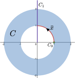
Figure 1. Example 4

Applying Theorem 2.2 to this optimal solution $(\bar{x},\bar{u})$ and using Remark 2.2$(c)$, we get the existence of an adjoint vector $\bar{p}:=(\bar{p}_{1},\bar{p}_{2})\in BV([0,\frac{\pi}{2}];\mathbb{R}^{2})$, a finite signed Radon measure $\bar{\nu}$ on $\left[0,\frac{\pi}{2}\right]$, $\bar{\xi}\in L^{\infty}([0,\tfrac{\pi}{2}];\mathbb{R}^{+})$, and $\lambda\geq 0$ such that, when incorporating equations (4.1) into $(i)$- $(vi)$, these latter simplify to the following:

1. $\|\bar{p}(\frac{\pi}{2})\|+\lambda=1.$

2. The admissibility equation holds, that is, for $t\in[0,\frac{\pi}{2}]$ a.e.,

   $$\begin{cases}\dot{\bar{x}}_{1}(t)=t-\bar{x}_{1}(t)-\bar{x}_{2}(t)-\bar{u}+6\bar{x}_{1}(t)\bar{\xi}(t),\\ \dot{\bar{x}}_{2}(t)=-t+\bar{x}_{1}(t)-\bar{x}_{2}(t)+\bar{u}+6\bar{x}_{2}(t)\bar{\xi}(t).\end{cases}$$

3. The adjoint equation is satisfied, that is, for $t\in[0,\frac{\pi}{2}]$,

   $$d\bar{p}(t) = \begin{pmatrix}1\;\;&-1\\ 1\;\;&1\end{pmatrix}\bar{p}(t)\hskip 0.42677ptdt\hskip 0.42677pt+\hskip 0.42677pt\bar{\xi}(t)\begin{pmatrix}8\bar{x}_{1}^{2}(t)-6\;\;&8\bar{x}_{1}(t)\bar{x}_{2}(t)\\ 8\bar{x}_{1}(t)\bar{x}_{2}(t)\;\;&8\bar{x}_{2}^{2}(t)-6\end{pmatrix}\bar{p}(t)\hskip 0.42677ptdt\hskip 0.42677pt$$

   $$- 6\hskip 0.42677pt\begin{pmatrix}\bar{x}_{1}(t)\\ \bar{x}_{2}(t)\end{pmatrix}d\bar{\nu}.$$

4. The complementary slackness condition is valid, that is,

   $$\bar{\xi}(t)(\bar{p}_{1}(t)\bar{x}_{1}(t)+\bar{p}_{2}(t)\bar{x}_{2}(t))=0,\>\>t\in\left[0,\tfrac{\pi}{2}\right]\;\mbox{a.e.}$$

5. The transversality condition holds: $-\bar{p}(\frac{\pi}{2})\in\lambda\{(0,1)\}+\{(\alpha,0)\in\mathbb{R}^{2}:\alpha\in\mathbb{R}\}$

6. $\max\{u(\bar{p}_{2}(t)-\bar{p}_{1}(t)):u\in[t,\pi]\}$ is attained at $\bar{u}(t)$ for $t\in[0,\frac{\pi}{2}]$ a.e.

From (4.1) combined with (b), we deduce that

$$\bar{\xi}(t)=\frac{1+(\bar{u}(t)-t)(\bar{x}_{1}(t)-\bar{x}_{2}(t))}{6},\;\textstyle\forall t\in[0,\frac{\pi}{2}].$$ (4.2)

On the other hand, the use of (d) and (4.1) in (c), yields that, for $t\in[0,\frac{\pi}{2}]$,

$$\begin{cases}d{\bar{p}}_{1}=(\bar{p}_{1}(t)-\bar{p}_{2}(t)-6\bar{\xi}(t)\bar{p}_{1}(t))\hskip 0.42677ptdt-6\bar{x}_{1}(t)\hskip 0.42677ptd\bar{\nu},\\ d{\bar{p}}_{2}=(\bar{p}_{1}(t)+\bar{p}_{2}(t)-6\bar{\xi}(t)\bar{p}_{2}(t))\hskip 0.42677ptdt-6\bar{x}_{2}(t)\hskip 0.42677ptd\bar{\nu}.\end{cases}$$ (4.3)

Now in order to exploit (f), we temporarily assume that

$$\bar{p}_{2}(t)<\bar{p}_{1}(t)\;\hbox{for}\;t\in[0,\tfrac{\pi}{2}]\;\hbox{a.e.,}$$ (4.4)

hoping to be able to find $\bar{p}_{1}$ and $\bar{p}_{2}$ satisfying this condition. In this case, $\bar{u}(t)=t$ for all $t\in[0,\frac{\pi}{2}]$, which gives using (4.2) that $\bar{\xi}(t)=\frac{1}{6}$ for all $t\in\left[0,\frac{\pi}{2}\right].$ Using these values of $\bar{u}$ and $\bar{\xi}$, and (4.1), we can solve for $(\bar{x}_{1},\bar{x}_{2})$ the two differential equations of (b) to obtain that

$$\textstyle\bar{x}(t)^{\mkern-1.5mu\mathsf{T}}=(\cos t,\sin t),\;\;\forall t\in[0,\frac{\pi}{2}].$$

Employing (a), (d), (e), and (4.3), a simple calculation yields that

$$\begin{cases}\lambda=\tfrac{3}{8}\;\,\hbox{and}\;\,\bar{p}(\tfrac{\pi}{2})=(\tfrac{1}{2},-\tfrac{3}{8}),\\[2.0pt] \bar{p}(t)^{\mkern-1.5mu\mathsf{T}}=\tfrac{1}{2}(\sin t,-\cos t)\;\hbox{on}\;[0,\tfrac{\pi}{2})\,\;\hbox{and}\;\,d\bar{\nu}=\tfrac{1}{16}\hskip 0.42677pt\delta_{\big{\{}\tfrac{\pi}{2}\big{\}}}\;\hbox{on}\;[0,\tfrac{\pi}{2}],\end{cases}\vspace{0.01cm}$$

where $\delta_{\{a\}}$ denotes the unit measure concentrated on the point $a$. Note that for all $t\in[0,\tfrac{\pi}{2}]$, we have $\bar{p}_{2}(t)<\bar{p}_{1}(t)$, and hence, the temporary assumption (4.4) is satisfied. Therefore, the above analysis, realized via Theorem 2.2, produces an admissible pair $(\bar{x},\bar{u})$, where

$$\textstyle\bar{x}(t)^{\mkern-1.5mu\mathsf{T}}=(\cos t,\sin t)\;\;\hbox{and}\;\;\bar{u}(t)=t,\;\;\forall t\in[0,\frac{\pi}{2}],$$

which is optimal for $(P)$.

References

- [1] C. Nour, V. Zeidan, A Control Space Ensuring the Strong Convergence of Continuous Approximation for a Controlled Sweeping Process, preprint (2023), arXiv:2301.00475.
- [2] J.J. Moreau, Rafle par un convexe variable, I, Trav. Semin. d’Anal. Convexe, Montpellier 1, Exposé 15, (1971), 36 pp.
- [3] J.J. Moreau, Rafle par un convexe variable, II, Trav. Semin. d’Anal. Convexe, Montpellier 2, Exposé 3, (1972), 43 pp.
- [4] J.J. Moreau, Evolution problem associated with a moving convex set in a Hilbert space, Journal of Differential Equations 26 (1977) 347-374.
- [5] L. Adam, J. Outrata, On optimal control of a sweeping process coupled with an ordinary differential equation, Discrete Contin. Dyn. Syst. B 19(9) (2014), 2709-2738.
- [6] T.H. Cao, B. Mordukhovich, Optimal control of a perturbed sweeping process via discrete approximations, Discrete Contin. Dyn. Syst. Ser. B 21 (2016), 3331-3358.
- [7] T.H. Cao, B. Mordukhovich, Optimality conditions for a controlled sweeping process with applications to the crowd motion model, Disc. Cont. Dyn. Syst. Ser. B 22 (2017), 267–306.
- [8] T.H. Cao, B. Mordukhovich, Optimal control of a nonconvex perturbed sweeping process, Journal of Differential Equations 266 (2019), 1003-1050.
- [9] M.d.R. de Pinho, M.M.A. Ferreira, G.V. Smirnov, Optimal Control Involving Sweeping Processes, Set-Valued Var. Anal. 27 no. 2 (2019), 523-548
- [10] M.d.R. de Pinho, M.M.A. Ferreira, G.V. Smirnov, Correction to: Optimal Control Involving Sweeping Processes, Set-Valued Var. Anal. 27 (2019), 1025-1027.
- [11] M.d.R. de Pinho, M.M.A. Ferreira, G.V. Smirnov, Optimal Control with Sweeping Processes: Numerical Method, J Optim Theory Appl 185 (2020), 845-858.
- [12] M.d.R. de Pinho, M.M.A. Ferreira, G.V. Smirnov, Necessary conditions for optimal control problems with sweeping systems and end point constraints, Optimization 71:11 (2021), 3363-3381.
- [13] V. Zeidan, C. Nour, H. Saoud, A nonsmooth maximum principle for a controlled nonconvex sweeping process, Journal of Differential Equations 269 (11) (2021), 9531-9582.
- [14] C. Nour, V. Zeidan, Optimal control of nonconvex sweeping processes with separable endpoints: Nonsmooth maximum principle for local minimizers, Journal of Differential Equations 318 (2022), 113-168.
- [15] C. Nour, V. Zeidan, Numerical solution for a controlled nonconvex sweeping process, IEEE Control Systems Letters vol. 6 (2022), 1190-1195.
- [16] D.G. Luenberger, Optimization by vector space methods, John Wiley & Sons, Inc. 1969.
- [17] F.H. Clarke, Optimization and Nonsmooth Analysis, John Wiley, New York, 1983.
- [18] P.D. Loewen, R.T. Rockafellar, The Adjoint Arc in Nonsmooth Optimization, Transactions of the American Mathematical Society 325 no. 1 (1991), 39-72.
- [19] R.A. Poliquin, R.T. Rockafellar, L. Thibault, Local differentiability of distance functions, Trans. Amer. Math. Soc. 352 (2000), 5231-5249.
- [20] J.-B. Hiriart-Urruty, Extension of Lipschitz functions, Journal of Mathematical Analysis and Applications 77 (1980) 539-554.
- [21] R.B. Vinter, Optimal Control, Birkhäuser, Systems and Control: Foundations and Applications, Boston, 2000.
- [22] D. Hoehener, Variational approach to second-order optimality conditions for control problems with pure state constraints, SIAM Journal on Control and Optimization 50:3 (2012), 1139-1173.