Maximizing soil moisture estimation accuracy through simultaneous hydraulic parameter estimation using microwave remote sensing: Methodology and application

Abstract

Improving the accuracy of soil moisture estimation is desirable from the perspectives of irrigation management and water conservation. To this end, this study proposes a systematic approach to select a subset of soil hydraulic parameters for estimation in large-scale agro-hydrological systems to enhance soil moisture estimation accuracy. The proposed method involves simultaneous estimation of the selected parameters and the entire soil moisture distribution of the field, taking into account soil heterogeneity and using soil moisture observations obtained through microwave radiometers mounted on a center pivot irrigation system. At its core, the proposed method models the field with the cylindrical coordinate version of the Richards equation and addresses the issue of parameter estimability (quantitative parameter identifiability) through the sensitivity analysis and orthogonal projection approaches. Additionally, the study assimilates remotely sensed soil moisture observations into the field model using the extended Kalman filtering technique. The effectiveness of the proposed methodology is demonstrated through numerical simulations and a real field experiment, with cross-validation results showing a 24-43% improvement in soil moisture estimation accuracy. Overall, the study highlights the potential of this method to enhance soil moisture estimation in large-scale agricultural fields.

Keywords: Sensitivity analysis, orthogonal projection, simultaneous state and parameter estimation, microwave remote sensing, center pivot irrigation systems.

1 Introduction

Agriculture is responsible for approximately 70% of all freshwater withdrawals, with irrigation activities consuming the majority of this resource, according to the United Nations [1]. Given the increasing scarcity of freshwater due to climate change and population growth, it is necessary to take steps to address the current water supply crisis. Improving the water-use efficiency in irrigation is one practical approach, as agriculture is a significant consumer of freshwater.

Closed-loop irrigation is one method of improving the water-use efficiency in agricultural irrigation [2]. To implement this approach, various soil moisture sensing techniques are required to provide the necessary soil moisture information for feedback control. While point sensors are reliable for sensing soil moisture, they face challenges in providing a detailed soil moisture characterization of large-scale fields. Alternatively, non-invasive sensing methods, such as microwave remote sensing, offer a more practical approach to characterize the soil water distribution of large-scale fields. Actually, microwave remote sensors have been demonstrated to quantitatively measure near-surface soil moisture. By installing these sensors on center pivot irrigation systems, it is possible to obtain soil water information by measuring the soil moisture content of the irrigated field as the pivot rotates. Center pivot irrigation systems are mechanized irrigation systems that irrigate crops in a circular pattern around a central pivot.

Soil moisture sensing techniques are limited in their ability to provide continuous and comprehensive characterization of soil moisture over time and space, leading to spatio-temporal gaps in soil moisture measurements. Designing a closed-loop irrigation system using sensor information that has spatio-temporal gaps often leads to inefficient irrigation, water wastage, or crop damage. Therefore, it is essential to ensure that the soil moisture information used for designing closed-loop irrigation systems is complete and reliable. One possible solution to address the data gaps is to use sequential data assimilation, a specific type of state estimation. Sequential data assimilation is a technique that combines observations from a limited number of sensors with a mathematical model to provide estimates of the state of a dynamic system. By employing a mathematical model, sequential data assimilation can interpolate or extrapolate the observed data to fill in gaps and provide a consistent estimate of the system’s state at all times. Various sequential data assimilation techniques, such as the extended Kalman filter (EKF) [3, 4], the ensemble Kalman filter (EnKF) [5, 6], the particle filter [7, 8] and the moving horizon estimator (MHE) [9, 10] are commonly used for soil moisture estimation. For instance, in [6], soil moisture estimates are obtained by assimilating L-band (1.4GHz) microwave radiobrightness observations into a land model using the EnKF. Similarly, in [9], soil moisture and parameter estimates are obtained by assimilating tensiometer measurements into the 1D Richards equation using the MHE. Recently, in [11], an information fusion system comprising of the cylindrical coordinate version of the Richards equation, the extended Kalman filter, and measurements from microwave remote sensors was developed to provide soil moisture estimates for fields equipped with center pivots.

Accurate soil moisture estimation using agro-hydrological models relies on soil hydraulic parameters, which are crucial inputs that influence the model’s accuracy in simulating soil moisture content. Therefore, obtaining an accurate quantification of these parameters is essential for soil moisture estimation. In an offline fashion, soil hydraulic parameters can be estimated by fitting a soil water retention curve under laboratory conditions. However, these laboratory methods are expensive and time-consuming. Furthermore, the parameters may vary over time, making an offline estimation method incapable of providing reasonably accurate estimates of the parameters. For large-scale fields, pedo-transfer functions (PTFs) can be used to estimate the soil hydraulic parameters by taking into account soil texture proportions, bulk density, and soil organic carbon content. However, studies have shown that PTF-generated soil hydraulic properties may lead to significant modelling errors [12, 13]. Parameter estimation can solve the aforementioned issues and provide an opportunity to estimate the hydraulic parameters of the soil while also estimating the soil moisture.

In dynamical systems, two main paradigms are mostly employed for estimating both states and parameters. The first paradigm is the joint/simultaneous method, which involves a simultaneous estimation of both the system states and model parameters using an augmented state vector that contains both. The second paradigm is the dual method, where states and parameters are estimated separately using two estimators or filters that run in parallel and exchange information at each iteration. While the joint approach is generally more accurate due to its ability to account for the interdependence between the system states and parameters, it increases the system order through the augmentation process, making it less computationally efficient than the dual approach [14]. For agro-hydrological systems, where accurate estimation of both soil moisture (the system states) and soil hydraulic parameters (the parameters) is critical, the joint/simultaneous approach is more appropriate since it can enhance the accuracy of both estimates by considering their interdependence. Soil moisture and hydraulic parameter estimation issues have been widely studied, with various methods proposed. For instance, in [15], the EnKF was employed to estimate the soil parameters that were augmented as extra states of the field model. Similarly, Medina et al. [16] coupled a standard Kalman filter for the retrieval of the states of the Richards equation and an unscented Kalman filter for retrieving the parameters of the van Genuchten-Maulem soil hydraulic functions. Lastly, in a different line of work, two EnKFs were designed to separately estimate soil moisture and the hydraulic parameters of a predictive hydrological model [17].

Despite the considerable success of the aforementioned works, studies on parameter estimability were not conducted prior to the implementation of the sequential data assimilation step. Prior to performing simultaneous state and parameter estimation for a given model, it is crucial to determine whether values for the selected set of model parameters can be uniquely estimated from a given data set and experimental conditions [18]. Evaluating parameter estimability is essential for at least one primary reason: non-estimable systems can pose a challenge for data assimilation techniques, leading to unreliable estimates of the non-estimable parameters [19].

Sensitivity analysis can be performed to determine if a model’s parameters can be accurately estimated for a given set of experimental conditions. This involves calculating a sensitivity coefficient matrix using a given input sequence, as described in Section 3.1. If the columns of the sensitivity matrix have full rank, then the parameters can be uniquely estimated. However, if the sensitivity matrix has a deficient rank, it is important to identify how many parameters can be uniquely estimated and which ones are the most identifiable parameters [18, 20].

Taking inspiration from the above, this research paper builds on our previous work [11], in which an information fusion system that incorporates the cylindrical coordinate version of the Richards equation, the extended Kalman filter, and measurements from microwave remote sensors was developed to estimate soil moisture of fields equipped with center pivots. The current study aims to improve the accuracy of the soil moisture estimates generated by this system. To achieve this, the sensitivity analysis and orthogonal projection approaches are employed to identify a subset of hydraulic parameters that can be uniquely estimated. The soil moisture information of the considered field and the selected hydraulic parameters are then estimated by assimilating the remotely sensed soil moisture content into the cylindrical coordinate version of the Richards equation using the extended Kalman filtering technique. Lastly, to further enhance the accuracy of the soil moisture and parameter estimates, the Kriging interpolation approach is used to interpolate the estimates of the estimable hydraulic parameters across the considered field. By simultaneously estimating a systematically selected subset of soil hydraulic parameters together with the soil moisture information of the field, the maximum information contained in the soil moisture observations can be extracted and the accuracy of the soil moisture estimates can be significantly enhanced.

This study is novel in its use of sensitivity analysis and orthogonal projection methods to evaluate the estimability of soil hydraulic parameters before the simultaneous estimation of soil moisture and hydraulic parameters from microwave sensor data collected on a center pivot irrigation system. Additionally, the paper makes contributions in the following areas:

1. Developing a procedure to construct and evaluate the output sensitivity matrix for systems with spatially varying measurements, such as microwave remote sensors mounted on a center pivot system.

2. Developing a modified version of the extended Kalman filtering algorithm that can handle changing estimable parameters over time in a computationally efficient manner.

3. Demonstrating the effectiveness of the proposed simultaneous state and parameter estimation method in improving the accuracy of soil moisture estimation in a real large-scale agricultural field.

This paper expands on the preliminary findings reported in [21, 22]. However, unlike [21, 22], this study provides more in-depth explanations and extensive simulation results for various scenarios to comprehensively evaluate the impact of sensitivity analysis on the performance of state and parameter estimation. Furthermore, a wider range of validation scenarios are included in the real case study to highlight the effectiveness of the proposed methodology.

2 Model Development

2.1 Field model

The system under study in this work is an agro-hydrological system equipped with a center pivot irrigation system as illustrated in Fig. 1. The dynamics of soil moisture in agro-hydrological systems can be modeled with the Richards equation [23]. To accurately depict the circular movement of the center pivot irrigation system, the cylindrical coordinate version of the Richards equation is employed as the field model in this work. The Richards equation in cylindrical coordinate form is expressed as [11]:

$$\frac{\partial\theta_{v}}{\partial t}=C(h)\frac{\partial h}{\partial t}=\frac{1}{r}\frac{\partial}{\partial r}\bigg{[}rK(h)\frac{\partial h}{\partial r}\bigg{]}+\frac{1}{r}\frac{\partial}{\partial\theta}\bigg{[}\frac{K(h)}{r}\frac{\partial h}{\partial\theta}\bigg{]}+\frac{\partial}{\partial z}\bigg{[}K(h)\bigg{(}\frac{\partial h}{\partial z}+1\bigg{)}\bigg{]}-S\left(h,z\right)$$ (1)

where $r,\theta,z$ represent the radial, azimuthal, and axial spatial variables, respectively. $h~{}(\text{m})$ is the pressure head, $\theta_{v}~{}(\text{m}^{3}\text{m}^{-3})$ is the volumetric soil moisture content, $t~{}(\text{s})$ is the temporal variable, $K(h)~{}(\text{ms}^{-1})$ is the unsaturated hydraulic water conductivity, $C(h)~{}(\text{m}^{-1})$ is the capillary capacity and $S\left(h,z\right)~{}(\text{m}^{3}\text{m}^{-3}\text{s}^{-1})$ is the root water extraction rate. The soil hydraulic functions $\theta_{v}(h)$, $K(h)$ and $C(h)$ in Eq. (1) are described by the Mualem-van Genucthen model [24]:

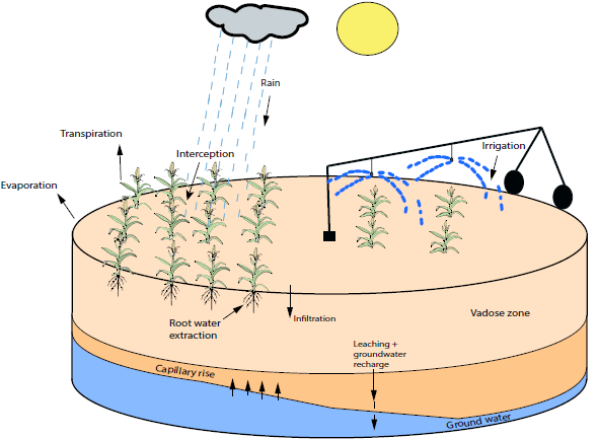
Figure 1: An agro-hydrological system [11].

$$\theta_{v}(h)=\theta_{r}+(\theta_{s}-\theta_{r})\bigg{[}\frac{1}{1+(-\alpha h)^{n}}\bigg{]}^{1-\frac{1}{n}}$$ (2)

$$K(h)=K_{s}\bigg{[}(1+(-\alpha h)^{n})^{-\big{(}\frac{n-1}{n}\big{)}}\bigg{]}^{\frac{1}{2}}\times\Bigg{[}1-\bigg{[}1-\Big{[}(1+(-\alpha h)^{n})^{-\big{(}\frac{n-1}{n}\big{)}}\Big{]}^{\frac{n}{n-1}}\bigg{]}^{\frac{n-1}{n}}\Bigg{]}^{2}$$ (3)

$$C(h)=\begin{cases}(\theta_{s}-\theta_{r})~{}\alpha n~{}\bigg{[}1-\frac{1}{n}\bigg{]}~{}(-\alpha h)^{n-1}\big{[}1+(-\alpha h)^{n}\big{]}^{-\big{(}2-\frac{1}{n}\big{)}}&h<0\\ S_{r}&h\geq 0\end{cases}$$ (4)

where $\theta_{s}~{}(\text{m}^{3}\text{m}^{-3})$, $\theta_{r}~{}(\text{m}^{3}\text{m}^{-3})$, $K_{s}~{}(\text{ms}^{-1})$, $S_{r}~{}(\text{m}^{{-1}})$ are the saturated volumetric moisture content, residual moisture content, saturated hydraulic conductivity and specific storage coefficient, respectively and $n$, $\alpha$ are curve-fitting soil hydraulic properties. The interested reader may refer to [11] for a thorough description of the agro-hydrological system equipped with a center pivot irrigation system and the derivation of Eq. (1).

2.2 Numerical Solution of the Field Model

Equation (1) is solved numerically for the following boundary conditions:

$$\frac{\partial h\left(r,\theta,z\right)}{\partial r} =0 \text{at}~{}\left(r=0,~{}\theta,~{}z\right)$$ (5)

$$\frac{\partial h\left(r,\theta,z\right)}{\partial r} =0 \text{at}~{}\left(r=H_{r},~{}\theta,~{}z\right)$$ (6)

$$\frac{\partial(h\left(r,\theta,z\right)+z)}{\partial z} =1 \text{at}~{}\left(r,~{}\theta,~{}z=0\right)$$ (7)

$$\frac{\partial(h\left(r,\theta,z\right))}{\partial z} =-1-\frac{u_{\text{irr}}-\text{EV}}{K(h)}~{}~{}~{}~{} \text{at}~{}\left(r,~{}\theta,~{}z=H_{z}\right)$$ (8)

where $H_{r}$ in Eq. (6) is the total radius of the field, $H_{z}$ in Eq. (8) is the length of the soil column. $u_{\text{irr}}$ (m/s) and EV (m/s) in Eq. (8) represents the irrigation and the potential evapotranspiration rates, respectively.

The two-point central difference scheme proposed in [11] is adopted as the solution method of Eq. (1) in this work. It is important to mention that the Richards equation is generally challenging to solve and its numerical solution can be unreliable under some conditions. To deal with these challenges, this work employs the following mechanisms during the numerical solution of Eq. (1). Some of the measures are enumerated below:

1. The inclusion of a specific storage coefficient $S_{r}$ of the soil medium in the parameterized equation of $C(h)$ to prevent the capillary capacity from assuming a value of 0 under wet conditions.

2. The adaptation of the numerical scheme such that only multiplication with $C(h)$ occurs so as to eliminate a degenerate solution when the capillary capacity assumes arbitrarily small values.

3. The use of an implicit scheme to approximate the temporal derivative in order to allow for reliable solutions under both saturated and unsaturated conditions.

The interested reader may refer to [11] for the full details of the mechanisms that can be used to guarantee a reliable numerical solution of Eq. (1). Note that the description of the root water extraction and potential evapotranspiration rates presented in [11] are also adopted in this work.

2.3 State-space Representation of the Field Model

After carrying out the numerical discretization, the field model can be expressed in state-space form as follows:

$$\dot{x}(t) =\mathcal{F}(x(t),u(t),{\bm{\Phi}})+\omega(t)$$ (9)

$$y(t) =\mathcal{H}({\mathcal{M}}(t)x(t),\bm{\Phi})+v(t)$$ (10)

In Eq. (9), $x(t)\in\mathbb{R}^{N_{x}}$ represents the state vector containing $N_{x}$ pressure head values. $N_{x}$ is the total number of discretization nodes of the system and is the product of the total number of discretization points in the radial, azimuthal, and axial directions, denoted by $N_{r}$, $N_{\theta}$, and $N_{z}$, respectively. That is, $N_{x}=N_{r}\times N_{\theta}\times N_{z}$. $u(t)\in\mathbb{R}^{N_{u}}$ and $\omega(k)\in\mathbb{R}^{N_{x}}$ represent the inputs and the model disturbances, respectively. To model field soil texture heterogeneity, it is considered that each node has its own hydraulic parameters including $\{K_{s},\theta_{s},\theta_{r},\alpha,n\}$. In Eqs. (9)-(10), $\bm{\Phi}\in\mathbb{R}^{N_{p}}$ represents the collection of all the soil hydraulic parameters of all the $N_{x}$ spatial node.

In Eq. (10), $y_{k}\in\mathbb{R}^{N_{y}}$, $v_{k}\in\mathbb{R}^{N_{y}}$ respectively denote the measurement vector and the measurement noise. Equation (10) is the general form of Eq. (2) since the microwave radiometers provide volumetric soil moisture observations. $\mathcal{M}(t)$ is a selection matrix which is used to select the measured states at time step $t$. It is imortant to add that the microwave radiometers measure the soil moisture content as the center pivot irrigates the field. Thus, the locations of the field at which the measurements are obtained change during the rotation cycle of the center pivot. This explains the explicit dependence of the selection matrix $\mathcal{M}(\cdot)$ on time $t$. $\mathcal{M}(t)$ is defined as $\mathcal{M}(t)=\frac{1}{N_{c}}\begin{bmatrix}I_{N_{y}\times N_{y}}(t)&\emptyset_{N_{y}\times(N_{x}-N_{y})}(t)\end{bmatrix}$, where $N_{c}$ is the number of nodes in the penetration depth of the microwave sensors and $N_{y}$ is the number of soil water content measurements obtained at time $t$. The matrix $\mathcal{M}(t)$ contains both the identity matrix $I$ and the zero matrix $\emptyset$. However, it is worth noting that the positions of these matrices in $\mathcal{M}(t)$ are not constant. The exact placement of $I$ and $\emptyset$ in $\mathcal{M}(t)$ may change depending on the specific locations of the measurements at time instant $t$. In other words, their positions in $\mathcal{M}(t)$ may be swapped.

3 Proposed Simultaneous State and Parameter Estimation

As has been mentioned earlier, the full soil moisture information of the field under study is essential for the design of a closed-loop irrigation system. To this end, we consider a setting in which the full soil moisture information (i.e. all the states of the field model) are estimated in the data assimilation step. Previous studies have investigated soil moisture estimation using the Richards equation and have shown that the entire state information of the equation can be recovered when at least one of these states is measured [25]. However, other studies that have attempted to perform state and parameter estimation of the Richards equation have found that augmenting all the nodal hydraulic parameters with the states results in a non-estimable augmented system [9]. One practical way to deal with a non-estimable augmented system is to select a subset of the parameters that are most critical to the behavior of the system. The selected parameters can then be augmented with the states so as to extract the maximal information contained in the measurements. In this work, the sensitivity analysis approach [20] and the orthogonal projection method [18] are used to determine the hydraulic parameters that have the greatest impact on the system behavior or model predictions.

In pursuit of the above, this section begins with a formal discussion of the sensitivity analysis method. Then an approach to construct the parametric output sensitivity matrix for a system with spatially varying measurements is presented. This is followed by a description of the orthogonal projection method. A modified version of the extended Kalman filtering technique, which is considered suitable for the system under study concludes this section.

3.1 Sensitivity Analysis

Sensitivity analysis measures how changes in the parameters of a system influence the outputs of the system. In essence, this approach involves the construction of the parametric output sensitivity matrix which is constructed by solving the dynamics of the original system in conjunction with the sensitivity dynamics. The sensitivity of the system state $x$ to the parameters $\bm{\Phi}$ can be expressed as follows [20]:

$$\frac{dx_{\bm{\Phi}}(t)}{dt} =\frac{\partial\mathcal{F}}{\partial x}x_{\bm{\Phi}}(t)+\frac{\partial\mathcal{F}}{{\partial\bm{\Phi}}}$$ (11)

$$y_{{\bm{\Phi}}}(t) =\frac{\partial\mathcal{H}}{\partial x}x_{\bm{\Phi}}(t)+\frac{\partial\mathcal{H}}{{\partial\bm{\Phi}}}$$ (12)

with $x_{\bm{\Phi}}(t)=\frac{\partial x(t)}{\partial\bm{\Phi}}$ and $y_{\bm{\Phi}}(t)=\frac{\partial y(t)}{\partial\bm{\Phi}}$. $x_{\bm{\Phi}}(t)\in\mathbb{R}^{N_{x}\times N_{p}}$ is initialized as $x_{\bm{\Phi}}(0)=\bm{0}_{N_{x}\times N_{p}}$ (a zero-matrix). The parametric output sensitivity matrix at time step $k$ can then be constructed as:

$$S_{y}(k)=\left[\begin{array}[]{cccc}\frac{\partial y_{1}(k)}{\partial\Phi_{1}}&\frac{\partial y_{1}(k)}{\partial\Phi_{2}}&\cdots&\frac{\partial y_{1}(k)}{\partial\Phi_{N_{p}}}\\ \frac{\partial y_{2}(k)}{\partial\Phi_{1}}&\frac{\partial y_{2}(k)}{\partial\Phi_{2}}&\cdots&\frac{\partial y_{2}(k)}{\partial\Phi_{N_{p}}}\\ \vdots&\vdots&\vdots&\vdots\\ \frac{\partial y_{N_{y}}(k)}{\partial\Phi_{1}}&\frac{\partial y_{N_{y}}(k)}{\partial\Phi_{2}}&\cdots&\frac{\partial y_{N_{y}}(k)}{\partial\Phi_{N_{p}}}\\ \end{array}\right]$$

where $y_{i}(k)$ is the $i^{\text{th}}$ observation at the $k^{\text{th}}$ time instant, and $\Phi_{j}$ denotes the $j^{\text{th}}$ elements in $\bm{\Phi}$.

Typically, the elements of $S_{y}(k)$ are of various physical dimensions and magnitudes, and a common procedure is to scale each element. This results in a scaled output sensitivity matrix $\tilde{S}_{y}(k)$, which is defined in this work as:

$$\tilde{S}_{y}(k)=\left[\begin{array}[]{cccc}\frac{\Phi_{1}}{y_{1}(k)}\frac{\partial y_{1}(k)}{\partial\Phi_{1}}&\frac{\Phi_{2}}{y_{1}(k)}\frac{\partial y_{1}(k)}{\partial\Phi_{2}}&\cdots&\frac{\Phi_{N_{p}}}{y_{1}(k)}\frac{\partial y_{1}(k)}{\partial\Phi_{N_{p}}}\\ \frac{\Phi_{1}}{y_{2}(k)}\frac{\partial y_{2}(k)}{\partial\Phi_{1}}&\frac{\Phi_{2}}{y_{2}(k)}\frac{\partial y_{2}(k)}{\partial\Phi_{2}}&\cdots&\frac{\Phi_{N_{p}}}{y_{2}(k)}\frac{\partial y_{2}(k)}{\partial\Phi_{N_{p}}}\\ \vdots&\vdots&\vdots&\vdots\\ \frac{\Phi_{1}}{y_{N_{y}}(k)}\frac{\partial y_{N_{y}}(k)}{\partial\Phi_{1}}&\frac{\Phi_{2}}{y_{N_{y}}(k)}\frac{\partial y_{N_{y}}(k)}{\partial\Phi_{2}}&\cdots&\frac{\Phi_{N_{p}}}{y_{N_{y}}(k)}\frac{\partial y_{N_{y}}(k)}{\partial\Phi_{N_{p}}}\\ \end{array}\right].$$

3.1.1 Output Sensitivity Matrix for Changing Measured Locations

As stated previously, the microwave radiometers considered in this study measure the soil moisture content during the rotation cycle of the center pivot. This means that the measured locations of the field change as the pivot rotates. Typically, the radiometers measure the moisture content of areas that have not yet been irrigated. Figure 2 illustrates the operation of a microwave radiometer mounted on a center pivot. As shown in the figure, if we assume that at time instant $k$ the currently irrigated nodes are represented by the blue dots, the radiometers will provide measurements of the nodes/locations represented by the red dots. It is important to note that as the pivot’s location shifts at time instant $k+1$, the measured nodes will also change.

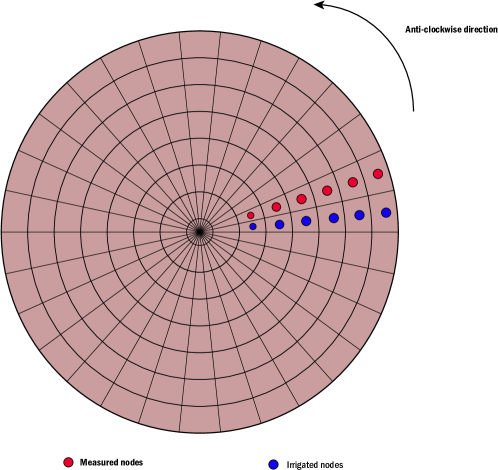
Figure 2: A schematic representation of center pivots equipped with microwave sensors.

When working with this type of system, it is not suitable to combine all the scaled output sensitivity matrices, which are constructed using all available measurements, into a single matrix. The reason for this is that the scaled sensitivity matrix that is computed at a specific sampling time $k$ only contains information about the measurements that are available at that particular step. When the measured states change during the next sampling time, the information contained in the scaled sensitivity matrix will also change accordingly. As a result, only those scaled sensitivity matrices that have identical measured states can be regarded as having similar information and can be grouped together. Therefore, the proposed approach is to group all the scaled output sensitivity matrices that share the same measured states into a single matrix.

The proposed methodology can be better understood through an illustrative example. In this instance, it is assumed that the field is partitioned into 40 sectors in the azimuthal direction. It is also presupposed that the sensitivity matrices of each sector are calculated at consecutive rotations. Based on the given assumptions, it can be deduced that for the first sector, the scaled output sensitivity matrices can be generated at time steps 1, 41, 81, 121, and so on. This leads to the creation of the output sensitivity matrices $\tilde{S}_{y}(1),\tilde{S}_{y}(41),\tilde{S}_{y}(81),\cdots$. These sensitivity matrices reflect how changes in the nodal hydraulic parameters of sector 1 affect its measurements. To obtain an overall sensitivity matrix for the first sector, all the sensitivity matrices of sector 1 are grouped together to for a single matrix, $\tilde{S}_{y}^{1}$. A similar approach can be used to calculate the overall scaled output sensitivity matrices for the other sectors, which can be represented as $\tilde{S}_{y}^{2},\tilde{S}_{y}^{3},...,\tilde{S}_{y}^{40}$.

A full rank scaled output sensitivity matrix is a sufficient condition for parameter estimability. By the principle of contraposition, this statement can be re-stated as: if the parameters are non-estimable, the scaled parametric output sensitivity matrix must be rank deficient. A full rank scaled sensitivity matrix is an indication that the considered hydraulic parameters are estimable, and they can be augmented with all the states of the field model during the data assimilation step. On the other hand, a rank deficient scaled sensitivity matrix indicates that some of the parameters are not estimable.

The singular value decomposition (SVD) is a well-known tool to assess the rank of a given matrix, and it is used in this work to determine the rank of the output sensitivity matrix [26]. For all intents and purposes, the SVD is a matrix factorization technique that decomposes a matrix $A$ into three matrices: $U$, $\Sigma$, and $V$ such that $A=U\Sigma V$. $U$ and $V$ are orthogonal matrices and $\Sigma$ is a diagonal matrix with non-negative real numbers on the diagonal. These non-negative real numbers are known as the singular values of the matrix $A$. The rank of matrix $A$ is equal to the number of non-zero singular values in $\Sigma$.

3.2 Orthogonal Projection Method for Parameter Selection

A rank deficient scaled output sensitivity matrix implies that some parameters in $\bm{\Phi}$ are non-estimable. To improve the accuracy of state and parameter estimation in such situations, it is necessary to focus on the most estimable parameters based on the measurements. This study utilizes the orthogonalization projection technique and the information from the scaled output sensitivity matrix to identify the most estimable elements of $\bm{\Phi}$. In essence, the orthogonal projection technique involves ranking the columns of the scaled sensitivity matrix according to their norm and linear independence. For a specific sector $i$ of the field, based on the constructed sensitivity matrix $\tilde{S}_{y}^{i}$, the detailed steps that are used to find the estimable parameters when the measurements are from sector $i$, are summarized as follows [18, 20]:

1. Evaluate the norm of each column of the scaled $\tilde{S}_{y}^{i}$, initialize $j=1$ and select the column $X_{j}$ with the largest norm.

2. Estimate the information $Z_{j}$ in $\tilde{S}_{y}^{i}$, expressed by $X_{j}$, and calculate the residual matrix $R_{j}$.

   $$Z_{j}=X_{j}(X_{j}^{T}X_{j})^{-1}\tilde{S}_{y}^{i}$$

   $$R_{j}=\tilde{S}_{y}^{i}-Z_{j}$$

3. Evaluate the norm of each column of the residual matrix $R_{j}$; select the column from $S_{y}^{i}$ that corresponds to the column with the largest norm in $R_{j}$ and add the selected column to $X_{j}$ to form $X_{j+1}$.

4. If the rank$\left(X_{j}\right)$ = rank$\left(\tilde{S}_{y}^{i}\right)$ or the largest norm of the columns of $R_{j}$ is smaller than a prescribed cut-off value, terminate the algorithm and the selected elements of $\bm{\Phi}$ correspond to the selected columns in $X_{j}$; otherwise, repeat Step 2 to Step 4 with $j\leftarrow j+1$.

The orthogonal projection method needs to be applied to all the scaled output sensitivity matrices constructed for the different sectors of the field to determine the corresponding most estimable parameters for measurements from different sectors. Additionally, to simplify the online estimation of states and selected parameters, the selection of the most-estimable soil hydraulic parameters can be performed offline based on extensive simulations. Note that when the measurements are from different sectors, the estimable parameters may change. That is, when the measurements are from sector $i$, the corresponding estimable parameters may be different from the estimable parameters when the measurements are from a different sector $j$ ($j\neq i$). However, all the potentially estimable parameters when the pivot rotates are collected in one vector and denoted by $\bm{\Phi}^{e}$ and the rest of the parameters are kept in $\bm{\Phi}^{ne}$.

3.3 Simultaneous State and Parameter Estimator

Prior to designing the simultaneous state and parameter estimator, the estimable parameters are added to all the original states of the field model to form an augmented system $x_{a}(t)=[x(t)~{}~{}\bm{\Phi}^{e}]$. The continuous-time system is also discretized so that the extended Kalman filter can be designed. The discrete time version of the augmented system, taking into account the non-estimable parameters can be expressed as follows:

$$x_{a}(k+1) =\mathcal{F}_{a}(x_{a}(k),u(k),\bm{\Phi}^{ne})+\omega_{a}(k)$$ (13)

$$y(k) =\mathcal{H}_{a}({\mathcal{M}_{a}}(k)x_{a}(k),\bm{\Phi}^{ne})+v(k)$$ (14)

It is important to note that the non-estimable parameters are assigned some nominal values during the estimation of $x_{a}$. However, at each sampling time, the Kriging interpolation approach will be used to update the elements of $\bm{\Phi}^{ne}$ after estimating the elements of $\bm{\Phi}^{e}$.

The extended Kalman filtering technique is chosen as the data assimilation technique in this work. In the first step of EKF, the filter is initialized with a guess of the augmented state $x_{a}(0)$ and its covariance matrix $P_{a}(0|0)$. The new augmented state $x_{a}$ and its covariance matrix $P_{a}$ are predicted using the nonlinear model at time $k+1$:

$$\hat{x}_{a}(k+1|k)=\mathcal{F}_{a}(\hat{x}_{a}(k|k),u(k),\bm{\Phi}^{ne})$$ (15)

$$P_{a}(k+1|k)=A(k)P_{a}(k|k)A(k)^{T}+Q$$ (16)

where $A(k)=\frac{\partial\mathcal{F}_{a}}{\partial x_{a}}\big{|}_{\hat{x}_{a}(k|k),~{}u(k)}$ and Q is the covariance matrix of the process disturbance $\omega_{a}$. The last step of EKF is updating the predicted augmented state and its covariance matrix using the observation $y(k+1)$ at time $k+1$ by:

$$\hat{x}_{a}(k+1|k+1)=\hat{x}_{a}(k+1|k)+G(k+1)[y(k+1)-\mathcal{H}_{a}({\mathcal{M}_{a}}(k)\hat{x}_{a}(k+1|k),\bm{\theta}^{ne})]$$ (17)

$$P_{a}(k+1|k+1)=[I-G(k+1)C(k+1)]P_{a}(k+1|k)$$ (18)

In the above equations, $G(k+1)$ is the Kalman gain matrix that can be calculated as:

$$G(k+1)=P_{a}(k+1|k)C^{T}(k+1)[C(k+1)P_{a}(k+1|k)C^{T}(k+1)+R]^{-1}$$ (19)

where $C(k+1)=\frac{\partial\mathcal{H}_{a}}{\partial x_{a}}\big{|}_{\hat{x}_{a}(k+1|k)}$ and $R$ is the covariance matrix of the measurement noise $v$. As stated earlier, the estimated hydraulic parameters $\bm{\Phi}^{e}$ and the Kriging interpolation approach will be employed to update the non-estimable parameters $\bm{\Phi}^{ne}$ at each sampling time, with the aim of enhancing the state estimation performance.

As explained earlier, the selected estimable hydraulic parameters may change over time. In the data assimilation step, the estimable parameter $\bm{\Phi}^{e}$ represents the complete set of estimable parameters derived from analyzing the sensitivity matrix constructed for each sector. During the data assimilation step, if an element of the estimable parameter vector $\bm{\Phi}^{e}$ is not being estimated at a particular time instant, the corresponding elements in $A(k)$ and $C(k)$ matrices are assigned a value of 0. This practice reflects the fact that such estimable parameters are not being estimated at that time instant. By adopting this approach, the data assimilation process can proceed effectively, while accommodating the changing nature of the estimable parameters over time, and preventing the need to store a large number of separate covariance matrices. Additionally, it also prevents the need to switch between different covariance matrices, and this leads to a more efficient implementation of the data assimilation algorithm.

Remark 1

To implement the EKF, CasADi [27] was used to symbolically calculate the required Jacobian matrices. Despite the Richards equation being highly nonlinear, the EKF was found to be less computationally expensive while providing accurate results compared to the EnKF. Due to limited knowledge of the initial estimate of the state in the real case study, a high initial covariance matrix was chosen for the EKF. This is generally feasible for the EKF, but not for the EnKF, where drawing ensembles from a distribution with a large variance can lead to improbable ensembles that the system model may be unable to propagate [28]. This can also degenerate the stability of the data assimilation process. However, for larger fields and cases where adequate knowledge of the initial estimate is available, the EnKF may be a better choice in terms of computational cost and data assimilation performance and it can be used to replace the EKF in the proposed state and parameter approach.

4 Simulated Case Study

This section evaluates the performance of the proposed state and parameter estimation method using simulated microwave sensor measurements. Initially, the system on which the simulations are based is described. Subsequently, a set of criteria is presented for evaluating the effectiveness of the proposed state and parameter estimator. Results of the sensitivity analysis and hydraulic parameter selection are also provided. Finally, the states estimation results of some selected states in the field model are presented to emphasize the benefits of the proposed method.

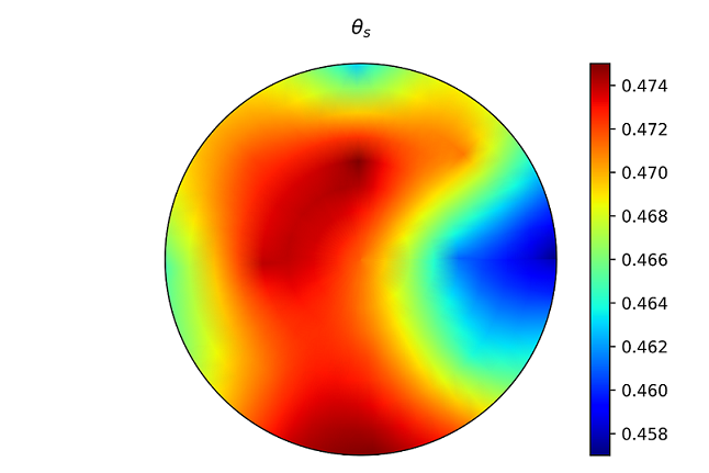
(a) $\theta_{s}~{}(m^{3}m^{-3})$

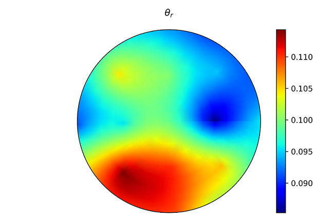
(b) $\theta_{r}~{}(m^{3}m^{-3})$

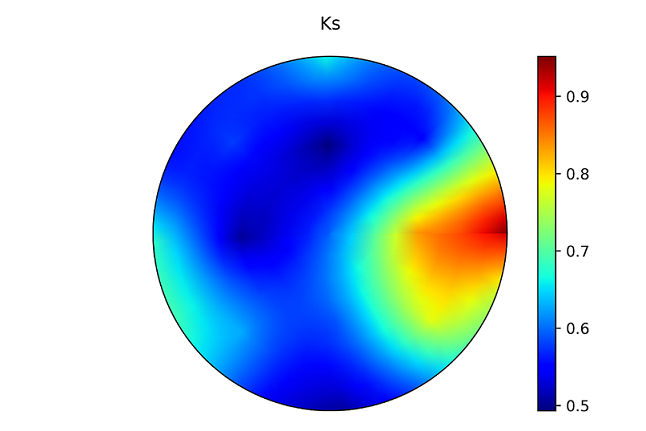
(c) $K_{s}~{}(cm{hr}^{-1})$

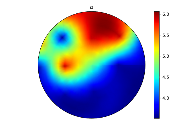
(d) $\alpha~{}(m^{-1})$

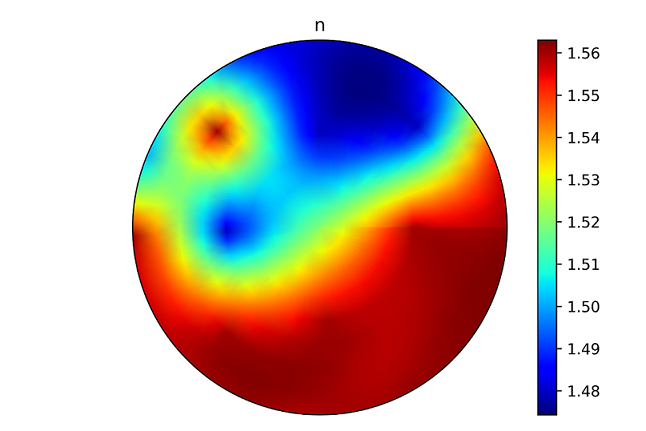
(e) $n~{}(-)$

Figure 3: Spatial distribution of the nominal soil hydraulic parameters.

4.1 System Description and Simulation Settings

In this investigation, a field with a radius of 290 meters and a depth of 0.3 meters is studied. The entire system is divided into $N_{x}=12000$ nodes, with 30 equally spaced nodes in the radial direction, 40 equally spaced nodes in the azimuthal direction, and 10 equally spaced nodes in the axial direction. Through extensive simulations, it was observed that mesh refinement in all three directions did not lead to significant changes in the state trajectories. Consequently, the discretization used is deemed to be an accurate numerical approximation of the field being investigated. The time step size used for the temporal discretization is 6 minutes. The study utilizes a heterogeneous field, and Fig. 3 shows the spatial distributions of the nominal hydraulic parameters used in the investigation. Note that vertically the soil properties are assumed to be the same. The initial pressure head of all nodes in the field model is randomly generated between -1.5 m and -1.35 m, and it varies from node to node. The center pivot employed in this study rotates at a speed of 0.011 m/s. The pivot is designed to deliver a constant irrigation rate of 3.6 mm/day and it irrigates the field in the first 8 hours of each day. A healthy barley crop at its development stage is assumed to be present in the investigated field. Consequently, this study employs crop coefficient values ranging from 0.75 to 0.96. Daily reference evapotranspiration values of 1.5 mm/day, 1.90 mm/day, 0.6 mm/day, 0.8 mm/day, and 2.40 mm/day are used as inputs. The simulation incorporates process noise and measurement noise, with zero mean and standard deviations of $1\times 10^{-6}$ m and $1\times 10^{-2}~{}\text{m}^{3}\text{m}^{-3}$, respectively. 30 measurements are employed at each sampling time to correct that elements of the augmented system in the update step of the EKF. It is important to mention that the location of these measurements change at each sampling time and the measurements employed in this study are simulated according to the procedure outlined in Section 3.1.1. Finally, the EKF is initialized as follows: $\hat{x}_{a}(0)\in[1.10x_{a}(0),1.15x_{a}(0)]$, where $\hat{x}_{a}(0)$ is the initial guess of the augmented system and $x_{a}(0)$ is the actual initial state of the augmented system.

Remark 2

By employing an implicit method to approximate the time derivative, the numerical method proposed in this study is considered to be unconditionally stable. This feature enables the use of larger time steps, although it should be noted that doing so may introduce a significant temporal truncation error, resulting in an imprecise solution. To address this, extensive simulations have been conducted to identify the appropriate time step that results in a small truncation error. The state trajectories are examined for various time step sizes, and a suitable time step is selected when further reducing its size does not produce a noticeable change in the state trajectories.

4.2 Evaluation criteria

The effectiveness of the proposed method in estimating soil moisture and soil hydraulic parameters is evaluated through three different cases. The first case (Case 1) involves only soil moisture estimation while considering uncertainty in the soil hydraulic parameters. In the second case (Case 2), all soil moisture and soil hydraulic parameters are estimated without considering the sensitivity analysis and selection of the estimable hydraulic parameters. In the third case (Case 3), the proposed method is used to simultaneously estimate both soil moisture and soil hydraulic parameters. To quantify the performance of each case, the root mean square error (RMSE) at a specific time and the average RMSE are used as evaluation metrics. The mathematical definitions of these metrics are provided as follows:

$$RMSE_{x_{a}}(k)=\sqrt{\frac{\sum_{i=1}^{n_{x_{a}}}(\hat{x}_{a,i}(k)-x_{a,i}(k))^{2}}{n_{x_{a}}}}$$ (20)

$$RMSE_{x_{a}}=\frac{\sum_{k=0}^{N_{sim}-1}RMSE_{x_{a}}(k)}{N_{sim}}$$ (21)

where RMSE${}_{x_{a}}(k)$ with $k=0,\cdots,N_{sim}-1$ shows the evolution of the RMSE value over time and RMSE${}_{x_{a}}$ shows the average value. $N_{sim}$ is the total number of time steps in the simulation period.

4.2.1 Determination of Significant Parameters

Based on the discretization of the field, the investigated field possesses 1200 nodes on its surface. Consequently, there exists $5\times 1200=6000$ hydraulic parameters in the model. The parameters of the field model $\bm{\Phi}$ can thus be represented as follows:

$$\bm{\Phi}=[K_{s,1},\theta_{s,1},\theta_{r,1},\alpha_{1},n_{1},\cdots,\\ K_{s,1200},\theta_{s,1200},\theta_{r,1200},\alpha_{1200},n_{1200}]^{T}\in\mathbb{R}^{6000}$$

According to the approach described in Section 3.1.1 for constructing output sensitivity matrices, the sectors comprising the field are considered for constructing the sensitivity matrices. For each sector, the sensitivity matrix consists of 6000 columns, representing the 6000 model parameters. By applying the SVD analysis to each sensitivity matrix, 6000 singular values, denoted as $\sigma_{1},\cdots,\sigma_{6000}$, can be obtained.

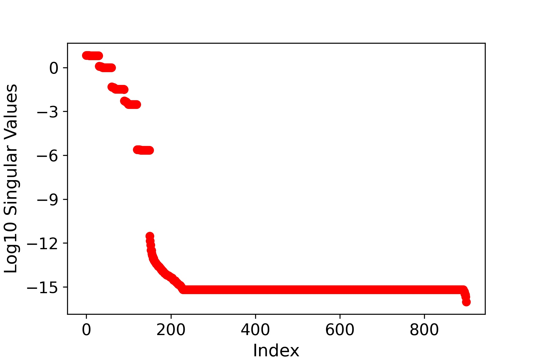
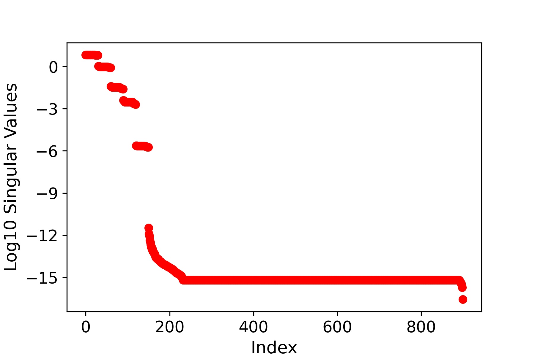
Figure 4: Plots of the logarithm of the singular values of scaled output sensitivity matrix for sectors (a) 1, (b) 10, (c) 25.

Figure 4 displays the first 900 biggest singular values of the overall sensitivity matrices for several sectors of the field on a logarithmic scale. Each subplot in Fig. 4 reveals a visible gap between $\sigma_{150}$ and $\sigma_{151}$, which spans roughly 5.8 decades on the logarithmic scale. This gap signifies a true zero value for the $150^{th}$ singular value, indicating a possible lack of estimability. Consequently, in the three depicted sectors, the sensitivity matrix has a rank of 150. This implies that, theoretically, only 150 out of the 6000 parameters can be uniquely estimated using the measurements at the specific sampling times. These same findings are also evident for remaining sectors of the field.

In this study, the termination criterion for the orthogonal projection method is the rank of the sensitivity matrix. Therefore, the next step is to identify the 150 most significant parameters that can be estimated. Upon conducting the orthogonal projection method, the 5 hydraulic parameters, namely $K_{s},~{}\theta_{s},~{}\theta_{r},~{}\alpha,$ and $n$, corresponding to the measured nodes of the field at sampling time $k$, are identified as the most estimable parameters. Thus, at each sampling time, the proposed method aims to estimate all original states of the field model along with $K_{s},~{}\theta_{s},~{}\theta_{r},~{}\alpha,$ and $n$ at the 30 measured nodes.

4.2.2 Estimation Results

Figure 5 displays the estimation results for the three cases. The evaluation metrics for the various cases are summarized in Table 1. From the table, it is evident that Case 1 produces the least accurate state estimates. Since the hydraulic parameters are not estimated in Case 1, no average RMSE values are reported for the hydraulic parameters in Case 1. Even though the hydraulic parameters are estimated together with the states in Cases 2 and 3, it is evident that estimating the non-estimable parameters together with the estimable ones degrades the estimation performance of the states. This follows from the fact that the average RMSE of the states in Case 3 is lower than the average RMSE of the states in Case 2. Similarly, estimating the non-estimable parameters results in a poorer estimation performance in terms of parameters, as Case 3 has a lower average RMSE in terms of the estimated hydraulic parameters compared to the corresponding average RMSE value of Case 2. The overall effect is that Case 3 possesses a lower average RMSE value in terms of the augmented system compared to Case 2. Figure 5 shows some of the actual and the estimated soil moisture trajectories in the three cases. A visual inspection of Fig. 5 further confirms that the proposed approach produces the most accurate state estimates.

Table 1: A summary of the evaluation metrics for the 3 cases.

Case	$\text{RMSE}_{x}~{}(\%)$	$\text{RMSE}_{\bm{\theta}}~{}(\%)$	$\text{RMSE}_{x_{a}}~{}(\%)$
1	26.29	n/a	26.29
2	24.19	14.20	24.00
3	16.60	13.90	16.44

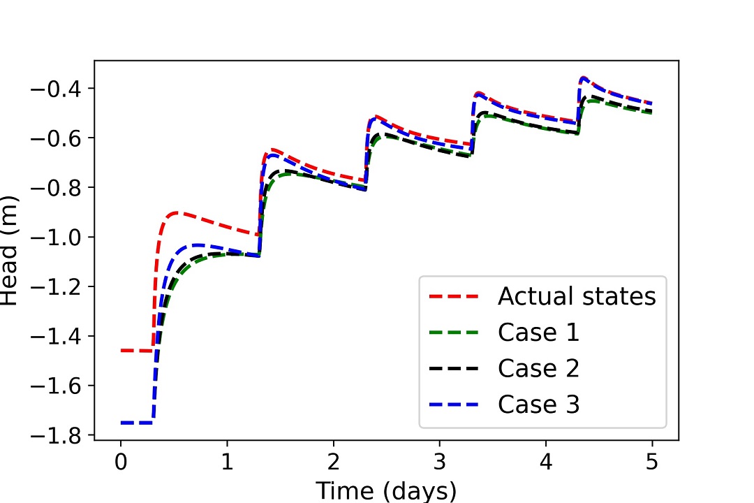
(a) Node 10700 at depth = 3.3 cm.

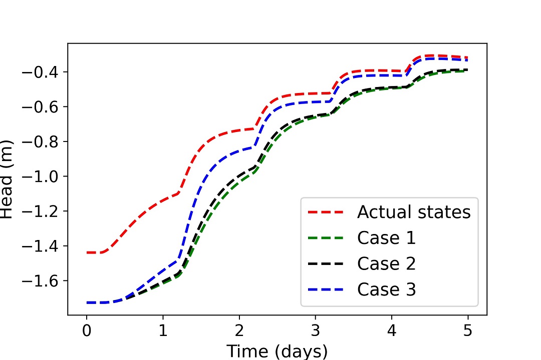
(b) Node 6601 at depth = 13.3 cm

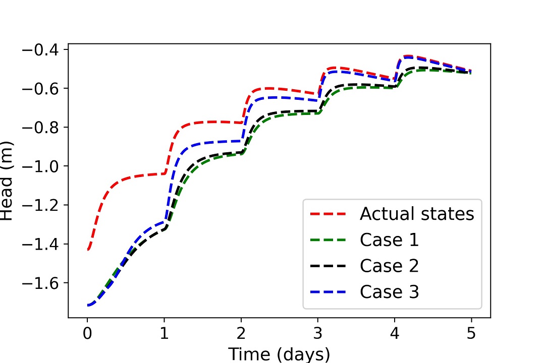
(c) Node 7200 at depth = 10 cm.

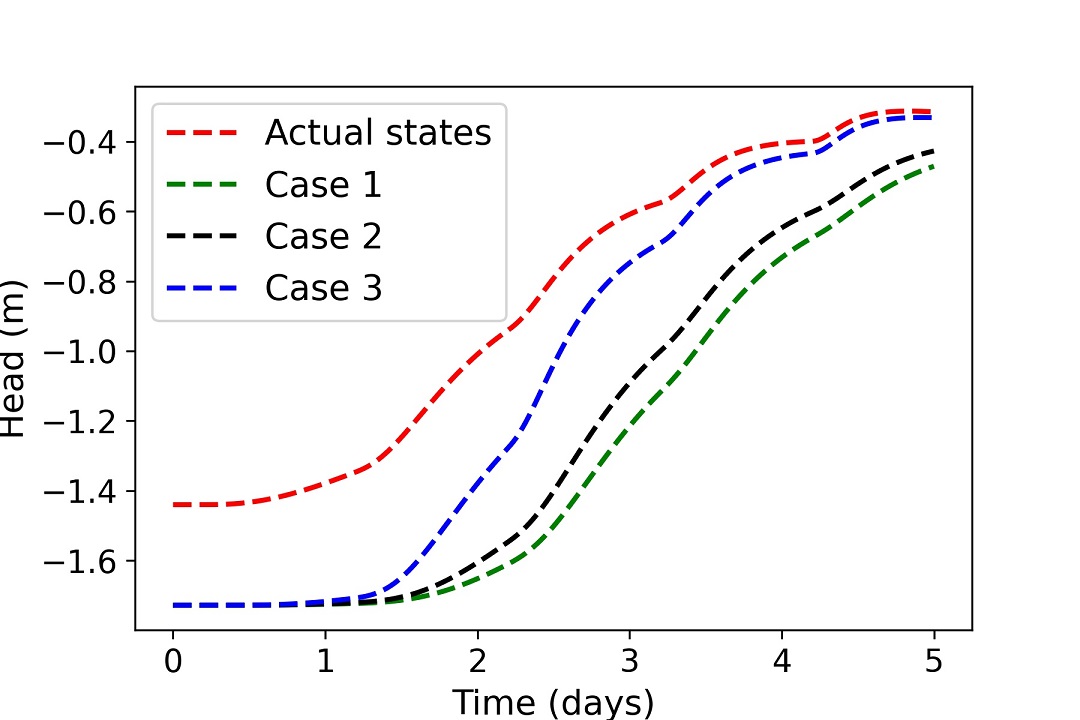
(d) Node 4150 at depth = 20 cm.

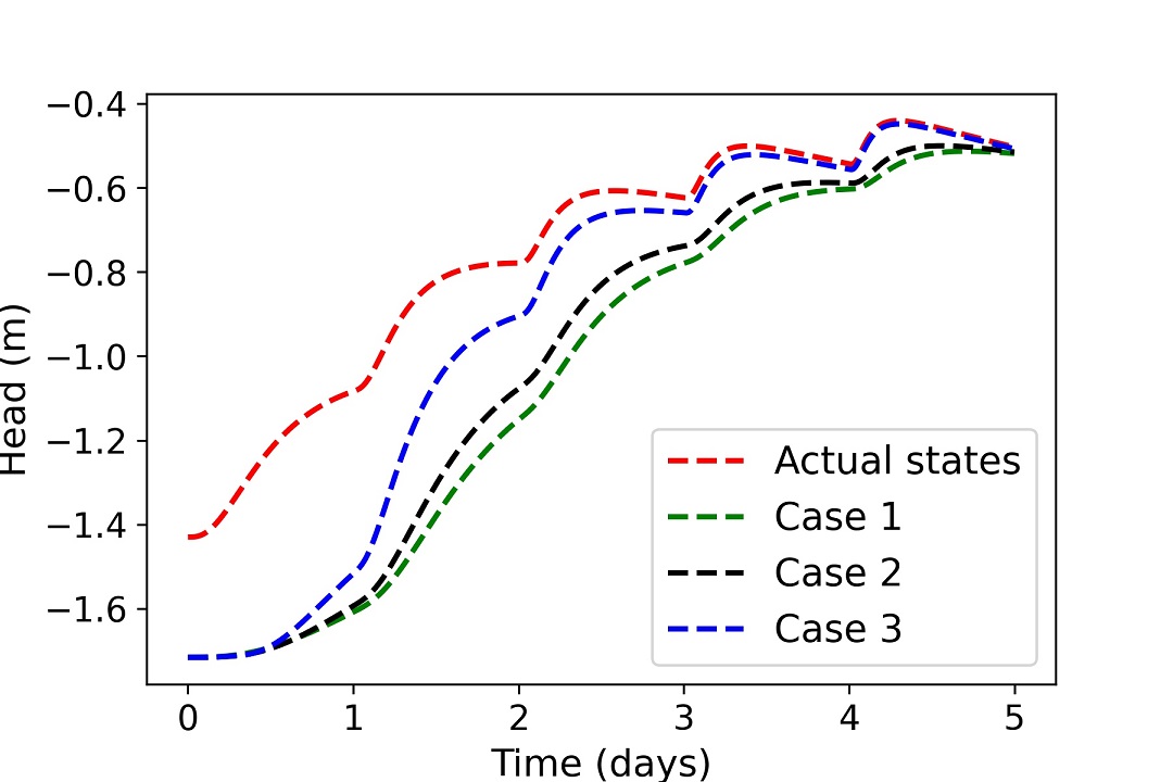
(e) Node 4840 at depth = 16.6 cm.

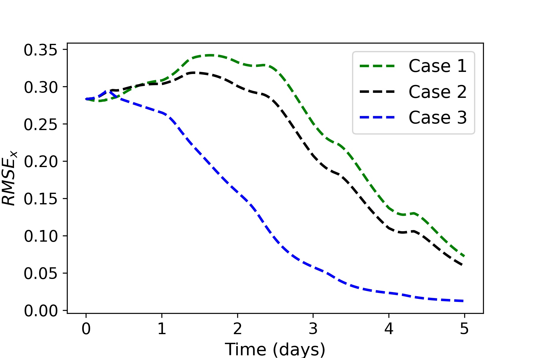
(f) RMSE

Figure 5: (a)-(e) Some selected trajectories of the actual states (red lines), estimated states in Case 1 (green lines), estimated states in Case 2 (black lines), and estimated states in Case 3 (blue lines). (f) Evolution of the RMSE of the original state vector during the simulation time in Case 1 (red lines), Case 2 (blue lines) and Case 3 (black lines).

.

5 Real Case Study

In this section, we demonstrate the utility, and performance of the proposed state and parameter estimation approach by considering microwave remote sensor measurements obtained from a field equipped with a center pivot irrigation system. The section begins with a description of the study area. Then, we present the numerical modeling of the investigated field, followed by a number of data pre-processing steps that generate an appropriate data representation for the state and parameter estimator. We examine the sensitivity analysis and the orthogonal projection approaches as applied to the field model and report the main outcomes of these steps. We introduce the design of the state and parameter estimator and outline the criteria used to assess the performance of our approach in the actual case study. Lastly, we present and discuss the primary results of the investigation.

5.1 Study Area

The study was conducted in 2021 at the Research Farm operated by Lethbridge College, which is located at 49.7230 °N and 112.8001 °W, east of the City of Lethbridge in Alberta, Canada. The center has an approximate area of 0.81 km² and an average elevation of 888 m. The primary soil type in the area is clayey loam with a few sand lenses. The layout of the center, delineated with the red rectangular blocks, is shown in Fig. 6. All three circular fields at the center are equipped with a center pivot irrigation system.

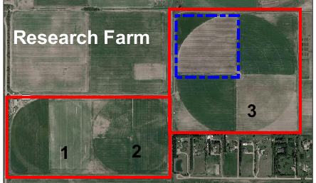
Figure 6: Layout of the research farm operated by Lethbridge College.

For the numerical investigation, a quadrant of Field 3 was selected, which is delineated by a blue dash-dotted rectangular block in Fig. 6. The soil moisture observations used in the study were obtained from microwave radiometers that were mounted on the center pivot of Field 3.

5.2 Numerical Modeling

The quadrant being studied has a total radius of 290 meters, a total depth of 0.6 meters, and a total angle of 0.5$\pi$ radians. To discretize the quadrant, the radius and angle are each divided into 30 and 17 equally spaced sectors, respectively. The number of nodes in the radial and azimuthal directions is chosen based on the distance between two consecutive microwave sensor measurements in the $r$ and $\theta$ directions. The depth $H_{z}$ is divided into 10 unequally spaced sectors with finer discretization near the surface and coarser discretization away from the surface. In total, the quadrant is discretized into $N_{x}=5100$ states. Further mesh refinement in the $z$ direction was found to have a negligible impact on the state trajectories. Hence, the adopted spatial discretization ensures an accurate numerical approximation of the investigated field. A time step size of 10 minutes is used for the temporal discretization of the field model. It is important to note that the time step size is determined according to Remark 2.

5.3 Data Preparation and Pre-processing

The study employed moisture content measurements taken from June 3rd, 2021 to July 22nd, 2021 in the investigated quadrant. Averagely, the microwave radiometers provided soil moisture measurements after every 30 seconds. Data assimilation was carried out using all the measurements obtained in June, while for the month of July, 80% of the measurements were used for data assimilation and the remaining measurements were used for validation purposes. To ensure an appropriate representation of data for the state and parameter estimator, the raw measurements were taken through a series of data pre-processing steps, which are listed and explained below.

1. Sorting measurements by date and time: Due to the large size of Field 3, the center pivot requires 2 to 3 days to complete its rotation cycle. Consequently, the water content measurements obtained from the microwave sensors at the end of the rotation cycle consist of measurements taken at various times over the course of 2 to 3 days. Therefore, it is important to sort the raw measurements initially by the date they were obtained. Then, all the measurements obtained on a particular day are arranged in ascending order according to their respective time.

2. Sorting measurements by quadrants: As this study focuses on one specific quadrant of Field 3, it is necessary to sort the measurements collected on a particular day by the quadrant in which they are located.

3. Inferring the movement of the center pivot: Since the microwave radiometers measure the soil water content of the field as the center pivot rotates, it is possible to infer the movement of the center pivot by analyzing how the measurement locations change over time. To accomplish this, the measurements are grouped based on a specific sampling time, denoted as $T_{s}$, so that the change in the measurement locations over time represents the circular movement of the pivot. Accurately determining the irrigated nodes of the quadrant at each sampling time requires inferring the movement of the center pivot. In this study, it was observed that grouping the measurements according to $T_{s}$ = 10 minutes accurately modeled the movement of the center pivot.

4. Dropping outliers: Finally, the data set is processed to identify and remove extreme soil moisture content measurements. The saturated and residual soil moisture contents of the dominant soil type in the investigated quadrant are used to identify these extreme measurements. Any measurement exceeding the saturated moisture content or falling below the residual soil moisture content is excluded from the data set.

5. Mapping measurements to the nodes of the field model: In order to associate each pre-processed measurement with a node in the field model, GPS coordinates are generated in a layout that matches the arrangement of nodes in the field model. When a measurement is received, the distances between its GPS coordinates and the generated coordinates are calculated, and the measurement is assigned to the node with the smallest distance from the measurement location.

Ancillary weather data such as the daily reference evapotranspiration (Fig. 7 B), daily average temperature (Fig. 7 A), and daily rain amount (Fig. 7 C), which are vital inputs to the field model were was obtained from the Alberta Information Service website. Similarly, the irrigation application depths (Fig. 7 C) for the simulation period were obtained from the Alberta Irrigation Center.

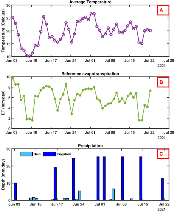
Figure 7: Trajectories of the daily average temperature (A), daily reference evapotranspiration (B), and daily precipitation rates (C) for the entire simulation period.

Finally, the following equation is used to determine the crop coefficient ($K_{c}$) values for barley [29] during the simulation period:

$$K_{c}(g)=0.04217+0.001508g+\left(4.89\times 10^{-6}\right)g^{2}-\left(8.69\times 10^{-9}\right)g^{3}+\left(2.49\times 10^{-12}\right)g^{4}$$ (22)

In Eq. 22, $g$ is the cumulative growing-degree days (GDD). GDD is calculated as follows:

$$\text{GDD}=\text{T}_{\text{avg}}-\text{T}_{\text{base}}$$ (23)

where $\text{T}_{\text{avg}}$ is the daily average/mean temperature and $\text{T}_{\text{base}}$ is the base temperature below which crop growth ceases (5°C).

5.4 Sensitivity Analysis and Orthogonal Projection

The output sensitivity matrices for each sector of the investigated quadrant were generated using the numerical model and nominal hydraulic parameters illustrated in Fig. 3. These matrices were created for all 2,550 hydraulic parameters associated with the nodes located on the field surface. After applying the orthogonal projection method to the rank-deficient, scaled output sensitivity matrices, it was determined that the most estimable parameters were the 5 hydraulic parameters associated with the measured locations on the field. The insights obtained from these results were used to determine the most estimable parameters at each time step during the real case study.

In this study, for the measurement sampling time of $T_{s}=10$ minutes, it was observed that there are between 10 and 60 measurements taken at each sampling time. By applying the results of the orthogonal projection, between 50 and 300 parameters can be uniquely estimated at each sampling time, together with the 5,100 states that make up the field model.

During the data assimilation step, the non-estimable parameters were assigned fixed values based on the dominant soil type of the investigated quadrant, specifically, hydraulic parameters for sandy clay loam were used. However, these values are updated using the Kriging interpolation method once the estimated parameters for the measured nodes are obtained to enhance the accuracy of soil moisture estimation.

5.5 State and Parameter Estimator Design

The state and parameter estimator is initialized with a covariance matrix, as explained in Section 3.3, that takes into account all the possible estimable parameters, which amounts to 2550 potential parameters. This approach eliminates the necessity of storing a large number of separate covariance matrices and also avoids the need to switch between different matrices, as previously mentioned.

The EKF is initialized with $\hat{x}_{a}(0)$ and a diagonal covariance matrix $P_{a}(0|0)$, which are set based on limited information available about $x_{a}(0)$. To account for the high uncertainty in $\hat{x}_{a}(0)$, the diagonal elements of $P_{a}(0|0)$ are assigned large values. Specifically, the elements corresponding to the states are initialized to 340, while those corresponding to the parameters are set to 6. The covariance matrices of process uncertainty $Q$ and measurement noise $R$ are considered as tuning parameters in this study. The diagonal elements of these matrices are gradually increased until a satisfactory agreement is achieved between the actual soil moisture measurements and their corresponding estimates obtained from the EKF filtering step. To be more specific, $Q$ is selected as $10I_{7,650}$, where $I_{7,650}$ is an identity matrix with a size of 7,650 $\times$ 7,650. Similarly, $R$ is chosen as $0.01I_{N_{y}}$, where $N_{y}$ represents the number of measurements obtained at each sampling time.

5.6 Evaluation Criteria

The performance of the state and parameter estimation approach is assessed with to types of cross-validation. In the first type, the measurements acquired at each sampling time are randomly split into a training set and a validation set. The estimates provided by the state and parameter estimator are compared with the measurements in the validation set. In essence, this type of validation seeks to evaluate the accuracy of the state estimates. In the second type of cross-validation, all the measurements obtained on a specific day during the simulation period (specifically July 21st, 2021) is used for validation. This is done by simulating the field model, taking into consideration the applied irrigation and the prevailing weather conditions observed on the 21st of July, 2021. In essence, this validation technique seeks to evaluate the predictive capability of the field model, after the estimated states and parameters have converged. The normalized root mean square error (NRMSE) is used to quantify the performance of the proposed approach. The NRMSE is calculated for the cross-validation step by comparing the estimated soil moisture content ($\hat{y}_{k}$) with the measured soil moisture content ($y_{k}$) values. The NRMSE is defined as:

$$\text{NRMSE}=\frac{1}{(y_{\text{max}}-y_{\text{min}})}\sqrt{\frac{\sum_{k=1}^{k=N}(y_{k}-\hat{y}_{k})^{2}}{N}}$$ (24)

where $N$ denotes the total number of measurements in the validation set, and $y_{\text{max}}$ and $y_{\text{min}}$ represent the maximum and minimum soil moisture content values in the validation set, respectively. A smaller value of NRMSE indicates a better match between the estimated and measured values.

To further highlight the advantages of estimating soil moisture and hydraulic parameters simultaneously, the results of two additional case studies are presented and analyzed together with the results of the proposed approach. The first case study (Case Study 1) involves estimating soil moisture using the hydraulic parameters of the dominant soil type in the investigated area, specifically sandy clay loam. The hydraulic properties of sandy clay loam are shown in Table 2. The second case study (Case Study 2) uses hydraulic parameters obtained from a soil texture survey conducted in the investigated area, where the parameters are interpolated at the 4 sampling locations using the Kriging method. The spatial distributions of the interpolated hydraulic parameters are depicted in Fig. 8. It is worth noting that the hydraulic parameters shown in Fig. 8 were obtained using PTFs, which took into account the percentages of sand, silt, and clay determined from the soil texture survey.

Table 2: The hydraulic parameters of sandy clay loam soil [30].

$K_{s}$ (m/s)	$\theta_{s}$ $(\text{m}^{3}/\text{m}^{3})$	$\theta_{r}$ $(\text{m}^{3}/\text{m}^{3})$	$\alpha$ (1/m)	$n$ (-)
$7.222\times 10^{-7}$	0.410	0.090	1.90	1.31

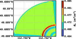
(a) Interpolated $\theta_{s}~{}(m^{3}m^{-3})$

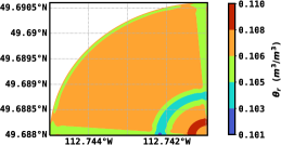
(b) Interpolated $\theta_{r}~{}(m^{3}m^{-3})$

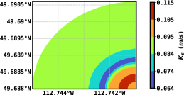
(c) Interpolated $K_{s}~{}(m{day}^{-1})$

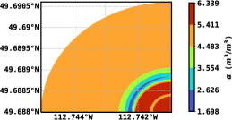
(d) Interpolated $\alpha~{}(m^{-1})$

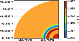
(e) Interpolated $n~{}(-)$

Figure 8: Spatially interpolated hydraulic parameters derived from field texture survey.

5.7 Performance Evaluation

The results of the first type of cross-validation performed on July 2nd and July 5th are shown in Figs. 9 and 10. In these figures, the inclusion of the $y=x$ line in all three case studies allows for the assessment of their respective performances. Based on the results, it is apparent that the proposed approach yields the most accurate estimates. The estimates obtained in Case Study 2, which involves soil moisture estimation using hydraulic parameters obtained from soil texture survey, follow closely in accuracy. Conversely, the soil moisture estimation that utilizes the parameters of the dominant soil type in the quadrant investigated generated the least accurate estimates. These findings confirm the importance of soil hydraulic parameters in state estimation, as their accuracy greatly influences the accuracy of soil moisture estimates. Notably, the closer the data points are to the $y=x$ line, which represents perfect agreement between the estimated and actual values, the more accurate the soil moisture estimates. Tables 3 and 4 display the NRMSE values obtained for each case study. It was observed that soil moisture estimation accuracy was significantly improved by estimating the soil hydraulic parameters. Specifically, the proposed approach led to improvements of 43% and 24% for July 2nd and July 5th, respectively, when compared to the case study that employed parameters of the dominant soil type in the quadrant investigated. These results further demonstrate that the proposed approach for estimating soil hydraulic parameters can significantly improve the accuracy of soil moisture estimates.

Table 3: NRMSEs of the Type 1 cross-validation performed on July 2nd, 2021.

Case Study	NRMSE
State estimation with parameters of the dominant soil type	0.28
State estimation with texture survey parameters	0.24
State and parameter estimation	0.16

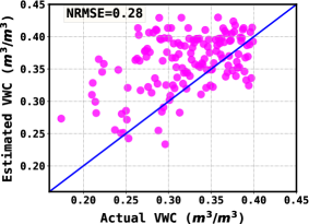
(a) Case 1

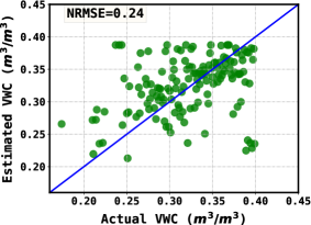
(b) Case 2

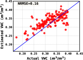
(c) Case 3

Figure 9: Cross-validation results for July 2nd, 2021.

Table 4: NRMSEs of the Type 1 cross-validation performed on July 5th, 2021.

Case Study	NRMSE
State estimation with parameters of the dominant soil type	0.29
State estimation with texture survey parameters	0.27
State and parameter estimation	0.22

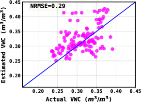
(a) Case 1

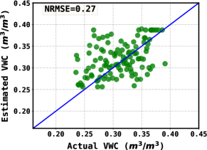
(b) Case 2

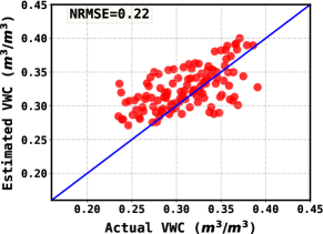
(c) Case 3

Figure 10: Cross-validation results for July 5th, 2021.

(a) Actual.

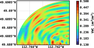
(b) Estimated.

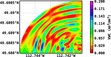
(c) Absolute error.

Figure 11: Cross validation using all the measurements obtained on July 21st, 2021 under Case 2.

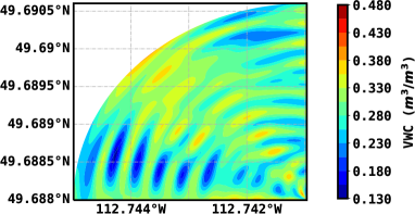
(a) Actual.

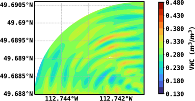
(b) Estimated.

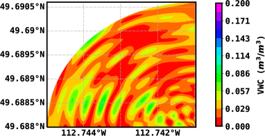
(c) Absolute error.

Figure 12: Cross validation using all the measurements obtained on July 21st, 2021 under Case 3.

The least accurate result, obtained from state estimation using the dominant soil type parameters, is not considered in the second type of cross-validation owing to the fact that it produced the least accurate results in the earlier cross-validation. The results of the validation for Case Study 2 and the proposed approach are illustrated in Figs. 11 and 12, and the NRMSE values are summarized in Table 5. From Figs. 11(c) and 12(c), it is evident that the proposed approach provides the most accurate model prediction, with a maximum absolute error of approximately 0.086 $\text{m}^{3}/\text{m}^{3}$ compared to the maximum absolute error of about 0.20 $\text{m}^{3}/\text{m}^{3}$ in the second case study. This observation is further supported by the NRMSE values summarized in Table 5, where the proposed approach yielded the smallest NRMSE value. Using the results obtained in Case Study 2 as a benchmark, it can be observed that the proposed approach is able to enhance the predictive capability of the field model by 50%. It should be noted that the NRMSE of the proposed approach is smaller in the second type of cross-validation compared to the first type since more samples were considered in the former. Generally, after the convergence of states and parameters, the estimation accuracy is expected to be better than the predictive accuracy of the field model.

The study evaluated the convergence and reliability of hydraulic parameter estimates, specifically the hydraulic conductivity. The estimated hydraulic conductivity was depicted spatially for two different dates using Fig. 13(a) for July 2nd and Fig. 13(b) for July 21st (the penultimate day of the simulation period). It is worth noting that all potentially estimable saturated hydraulic conductivities were initially set to a uniform value of 0.086 $\text{m}/\text{day}$. The results indicated that after incorporating the field measurements into the model using the proposed method, the estimated conductivities deviated from their initial values and eventually converged to values ranging from 0.295 to 0.301 $\text{m}/\text{day}$. A slight difference in estimated $K_{s}$ values was observed between the depicted days in Figs. 13(a) and 13(b), indicating that the estimated $K_{s}$ converged. To verify the reliability of the estimated $K_{s}$, laboratory-determined $K_{s}$ values for five randomly sampled points were compared with the estimated $K_{s}$ values, and a good agreement was found with the mean value (0.39 $\text{m}/\text{day}$) of these laboratory-determined $K_{s}$ values.

Table 5: NRMSEs of the Type 2 cross-validation performed on July 21st, 2021.

Case Study	NRMSE
State estimation with texture survey parameters	0.24
State and parameter estimation	0.12

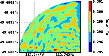
(a) Estimated $K_{s}$ on July 02, 2021.

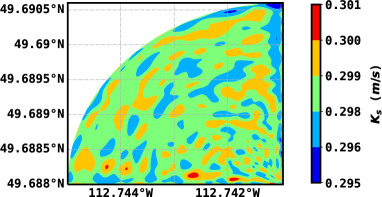
(b) Estimated $K_{s}$ on July 21, 2021.

Figure 13: Estimated $K_{s}$ (m/day).

6 Conclusion

In this paper, a systematic method to simultaneously estimate soil moisture and soil hydraulic parameters in large-scale agro-hydrological systems with soil heterogeneity by utilizing soil moisture observations acquired through microwave radiometers installed on center pivot irrigation systems was proposed. Basically, the proposed approach involves modeling the field under study with the cylindrical coordinate version of the Richards equation, employing the sensitivity analysis and the orthogonal projection methods to address issues of parameter estimability, and assimilating the remotely sensed moisture observations into the field model using the extended Kalman filtering technique. Technical issues, such as constructing the output sensitivity matrix to handle spatially varying measurements and modifying the extended Kalman filter to accommodate changing estimable parameters over time, were addressed.

The outcomes of sensitivity analysis and orthogonal projection methods show that the hydraulic parameters of the measured nodes in the field model are the most estimable, and these parameters, along with all states of the field model, can be reliably estimated. Simulated and real case studies were conducted, revealing that the proposed approach enhances the accuracy of soil moisture estimation while providing reliable estimates of hydraulic parameters. Therefore, it can be concluded that the proposed method can provide accurate soil moisture information for the design of closed-loop irrigation.

Despite the promising results, other modifications or directions are worth exploring. To increase the number of estimable hydraulic parameters, it will be of vital importance to incorporate measurements from fixed point sensors in the proposed framework. This modification can affect the location of the estimable hydraulic parameters, and extensive simulations that employ the sensitivity analysis and orthogonal projection methods have to be carried out to determine the number and location of the estimable parameters. Alternative ways must also be developed to construct the output sensitivity matrix when measurements from fixed point sensors are considered in the proposed framework. Finally, scaling the proposed approach to larger fields is still a challenge, and structure and topology preserving model reduction techniques can be explored to enhance the computational efficiency of the proposed method. Parameter estimability studies are also needed to assess the impact of the reduced model on the number and location of the most estimable parameters.

7 Acknowledgements

Financial support from Natural Sciences and Engineering Research Council of Canada and Alberta Innovates is gratefully acknowledged.

References

- [1] UN Water, WWAP (United Nations World Water Assessment Programme), Facing the challenges, Case Studies and Indicators. Paris, UNESCO, 2015.
- [2] S. L. Shah, B. R. Bakshi, J. Liu, C. Georgakis, B. Chachuat, R. D. Braatz, and Y. Brent, “Meeting the challenges of water sustainability: the role of process systems engineering,” AIChE Journal, vol. 67, p. e17113, 2021.
- [3] H. Lü, Z. Yu, Y. Zhu, S. Drake, Z. Hao, and E. A. Sudicky, “Dual state-parameter estimation of root zone soil moisture by optimal parameter estimation and extended kalman filter data assimilation,” Advances in Water Resources, vol. 34, no. 3, pp. 395–406, 2011.
- [4] J. M. Sabater, L. Jarlan, J.-C. Calvet, F. Bouyssel, and P. De Rosnay, “From near-surface to root-zone soil moisture using different assimilation techniques,” Journal of Hydrometeorology, vol. 8, no. 2, pp. 194–206, 2007.
- [5] H. Medina, N. Romano, and G. B. Chirico, “Kalman filters for assimilating near-surface observations into the Richards equation – Part 2: A dual filter approach for simultaneous retrieval of states and parameters,” Hydrology and Earth System Sciences, vol. 18, no. 7, pp. 2521–2541, 2014.
- [6] R. H. Reichle, D. B. McLaughlin, and D. Entekhabi, “Hydrologic data assimilation with the ensemble Kalman filter,” Monthly Weather Review, vol. 130, no. 1, pp. 103–114, 2002.
- [7] C. Montzka, H. Moradkhani, L. Weihermüller, H.-J. H. Franssen, M. Canty, and H. Vereecken, “Hydraulic parameter estimation by remotely-sensed top soil moisture observations with the particle filter,” Journal of Hydrology, vol. 399, no. 3-4, pp. 410–421, 2011.
- [8] M. Pan, E. F. Wood, R. Wójcik, and M. F. McCabe, “Estimation of regional terrestrial water cycle using multi-sensor remote sensing observations and data assimilation,” Remote Sensing of Environment, vol. 112, no. 4, pp. 1282–1294, 2008.
- [9] S. Bo, S. R. Sahoo, X. Yin, J. Liu, and S. L. Shah, “Parameter and state estimation of one-dimensional infiltration processes: A simultaneous approach,” Mathematics, vol. 8, no. 1, p. 134, 2020.
- [10] S. Bo and J. Liu, “A decentralized framework for parameter and state estimation of infiltration processes,” Mathematics, vol. 8, no. 5, p. 681, 2020.
- [11] B. T. Agyeman, S. Bo, S. R. Sahoo, X. Yin, J. Liu, and S. L. Shah, “Soil moisture map construction by sequential data assimilation using an extended kalman filter,” Journal of Hydrology, vol. 598, p. 126425, 2021.
- [12] Y. Li, D. Chen, R. White, A. Zhu, and J. Zhang, “Estimating soil hydraulic properties of fengqiu county soils in the north china plain using pedo-transfer functions,” Geoderma, vol. 138, no. 3-4, pp. 261–271, 2007.
- [13] M. Soet and J. Stricker, “Functional behaviour of pedotransfer functions in soil water flow simulation,” Hydrological processes, vol. 17, no. 8, pp. 1659–1670, 2003.
- [14] A. Hegyi, D. Girimonte, R. Babuska, and B. De Schutter, “A comparison of filter configurations for freeway traffic state estimation,” in 2006 IEEE Intelligent Transportation Systems Conference, pp. 1029–1034, IEEE, 2006.
- [15] C. Li and L. Ren, “Estimation of unsaturated soil hydraulic parameters using the ensemble kalman filter,” Vadose Zone Journal, vol. 10, no. 4, pp. 1205–1227, 2011.
- [16] H. Medina, N. Romano, and G. Chirico, “Kalman filters for assimilating near-surface observations into the richards equation–part 2: A dual filter approach for simultaneous retrieval of states and parameters,” Hydrology and Earth System Sciences, vol. 18, no. 7, pp. 2521–2541, 2014.
- [17] H. Moradkhani, S. Sorooshian, H. V. Gupta, and P. R. Houser, “Dual state–parameter estimation of hydrological models using ensemble kalman filter,” Advances in Water Resources, vol. 28, no. 2, pp. 135–147, 2005.
- [18] K. Z. Yao, B. M. Shaw, B. Kou, K. B. McAuley, and D. Bacon, “Modeling ethylene/butene copolymerization with multi-site catalysts: parameter estimability and experimental design,” Polymer Reaction Engineering, vol. 11, no. 3, pp. 563–588, 2003.
- [19] O.-T. Chis, J. R. Banga, and E. Balsa-Canto, “Structural identifiability of systems biology models: a critical comparison of methods,” PloS one, vol. 6, no. 11, p. e27755, 2011.
- [20] J. Liu, A. Gnanasekar, Y. Zhang, S. Bo, J. Liu, J. Hu, and T. Zou, “Simultaneous state and parameter estimation: the role of sensitivity analysis,” Industrial & Engineering Chemistry Research, vol. 60, no. 7, pp. 2971–2982, 2021.
- [21] E. Orouskhani, B. T. Agyeman, and J. Liu, “Simultaneous estimation of soil moisture and hydraulic parameters for precision agriculture. part a: Methodology,” in 2022 IEEE International Symposium on Advanced Control of Industrial Processes (AdCONIP), pp. 12–17, IEEE, 2022.
- [22] B. T. Agyeman, E. Orouskhani, and J. Liu, “Simultaneous estimation of soil moisture and hydraulic parameters for precision agriculture. part b: Application to a real field,” in 2022 IEEE International Symposium on Advanced Control of Industrial Processes (AdCONIP), pp. 18–23, IEEE, 2022.
- [23] L. A. Richards, “Capillary conduction of liquids through porous mediums,” Physics, vol. 1, no. 5, pp. 318–333, 1931.
- [24] M. T. Van Genuchten, “A closed-form equation for predicting the hydraulic conductivity of unsaturated soils,” Soil Science Society of America Journal, vol. 44, no. 5, pp. 892–898, 1980.
- [25] S. R. Sahoo, X. Yin, and J. Liu, “Optimal sensor placement for agro-hydrological systems,” AIChE Journal, vol. 65, no. 12, p. e16795, 2019.
- [26] J. Stigter, D. Joubert, and J. Molenaar, “Observability of complex systems: Finding the gap,” Scientific Reports, vol. 7, no. 1, pp. 1–9, 2017.
- [27] J. A. Andersson, J. Gillis, G. Horn, J. B. Rawlings, and M. Diehl, “Casadi: a software framework for nonlinear optimization and optimal control,” Mathematical Programming Computation, vol. 11, pp. 1–36, 2019.
- [28] G. Chirico, H. Medina, and N. Romano, “Kalman filters for assimilating near-surface observations into the richards equation–part 1: Retrieving state profiles with linear and nonlinear numerical schemes,” Hydrology and Earth System Sciences, vol. 18, no. 7, pp. 2503–2520, 2014.
- [29] D. R. Bennett and T. E. Harms, “Crop yield and water requirement relationships for major irrigated crops in southern alberta,” Canadian Water Resources Journal, vol. 36, no. 2, pp. 159–170, 2011.
- [30] R. F. Carsel and R. S. Parrish, “Developing joint probability distributions of soil water retention characteristics,” Water Resources Research, vol. 24, no. 5, pp. 755–769, 1988.