$T-\mu$ quark matter phase transitions and critical end point in nonlocal PNJL models under a strong magnetic field

Abstract

We study the $T-\mu$ phase diagram of quark matter under the influence of a strong uniform magnetic field in the framework of a nonlocal extension of the Polyakov–Nambu–Jona-Lasinio model (PNJL). The existence of a critical end point (CEP) is found for the whole considered range of the magnetic field (up to 1 GeV²). We analyze the location of this CEP as a function of the external field and discuss the presence of inverse magnetic catalysis for nonzero chemical potentials. Our results show that the temperature of the CEP decreases with the magnetic field, in contrast to the behavior observed in local NJL/PNJL models.

I Introduction

The study of the QCD phase diagram under the influence of a strong external magnetic field has captivated significant attention in recent years (Kharzeev et al., 2013; Andersen et al., 2016; Miransky and Shovkovy, 2015). This is due in part to the fact that the subject has applications in various fields such as cosmology, heavy ion collisions and compact stars physics. In fact, it has been argued (Vachaspati, 1991) that extremely high magnetic fields (reaching orders of magnitude of about $10^{20}$ G) could have existed during the cosmological electroweak phase transition; in addition, in ultra-peripheral heavy-ion collisions the generated magnetic fields are shown to be proportional to the collision energy, reaching up to $\sim 5\times 10^{19}$ G (Deng and Huang, 2012), while in an astrophysical scenario, the magnetic field on the surface of magnetars is estimated to be of the order of $10^{14}$ G (Duncan and Thompson, 1992), and significantly higher values are expected to be found in the deep interior of these objects. Since the order of magnitude of such huge magnetic fields is comparable to the QCD confining scale squared ($|eB|\gtrsim\Lambda_{\rm QCD}^{2}$ for $|B|\gtrsim 10^{19}$ G), the above scenarios offer interesting opportunities to probe the QCD phase diagram in the region of deconfinement and chiral symmetry restoration transitions.

Due to the nonperturbative character of strong interactions in this regime of interest, one is lead either to use lattice QCD (LQCD) techniques or to rely on effective theories that could capture the main features of QCD phenomenology showing at the same time consistency with LQCD results. Among these effective theories, the Nambu-Jona-Lasinio (NJL) model (Nambu and Jona-Lasinio, 1961a, b) is one of the most widely used approaches. In this effective chiral quark model, quarks interact through local four-point vertices, leading to the spontaneous breakdown of chiral symmetry for a sufficiently large coupling strength (Vogl and Weise, 1991; Klevansky, 1992; Hatsuda and Kunihiro, 1994). In fact, it has been pointed out that the model can be improved by considering nonlocal separable interactions, which arise naturally in several effective approaches to QCD and lead to a better agreement with LQCD calculations (Schmidt et al., 1994; Burden et al., 1997; Bowler and Birse, 1995; Ripka, 1997). A recent review that discuss the features of nonlocal NJL models, including the analysis of strong interaction matter under extreme conditions, can be found in Ref. (Dumm et al., 2021).

In this work we study the hadron-quark QCD phase diagram in the context of a nonlocal two-flavor NJL model (General et al., 2001; Gomez Dumm and Scoccola, 2002; Dumm et al., 2006) that also includes the interaction between the quarks and the Polyakov loop (’t Hooft, 1978; Polyakov, 1978; Meisinger and Ogilvie, 1996; Fukushima, 2004; Megias et al., 2006; Ratti et al., 2006a; Roessner et al., 2007; Mukherjee et al., 2007; Sasaki et al., 2007). This so-called nonlocal Polyakov-Nambu-Jona-Lasinio model (nlPNJL) (Contrera et al., 2008; Hell et al., 2009; Carlomagno et al., 2013) provides an order parameter for the confinement/deconfinement transition, and leads to a critical temperature for chiral symmetry restoration that is found to be in good agreement with LQCD results (Karsch and Laermann, 2003). Noticeably, nonlocal PNJL models show the interesting feature of being able to reproduce in a naturally way the effect known as inverse magnetic catalysis (IMC) (Pagura et al., 2017; Dumm et al., 2017): while at zero temperature the presence of a strong magnetic field leads to an enhancement of the quark-antiquark chiral condensate (favouring, or “catalizing”, the breakdown of chiral symmetry), this behaviour becomes the opposite if the temperature gets significantly increased. The observation of IMC from LQCD calculations (Bali et al., 2012a, b) represents a challenge for most naive effective approaches for low energy QCD (including the usual local NJL model), in which this effect is not found (Andersen et al., 2016; Kharzeev et al., 2013; Miransky and Shovkovy, 2015).

In the framework of nlPNJL models, we concentrate here on the study of the deconfinement and chiral restoration transitions in the $T-\mu$ phase diagram (where $T$ is the temperature and $\mu$ the quark chemical potential), considering the presence of an external uniform and static magnetic field $\vec{B}$. This has been previously addressed in the context of the Ginzburg-Landau formalism, the linear sigma model, and various versions of local NJL-like models, see Refs. (Ruggieri et al., 2014; Inagaki et al., 2004; Avancini et al., 2012; Ferrari et al., 2012; Costa et al., 2014, 2015; Rechenberger, 2017; Ferreira et al., 2018a; Tawfik et al., 2018; Ferreira et al., 2018b; Ayala et al., 2021). Our analysis within the nonlocal PNJL approach can be viewed as an extension of two previous works, Refs. (Dumm et al., 2017) and (Ferraris et al., 2021), in which systems at nonzero temperature and nonzero density were separately considered. A previous analysis has been also done within the nonlocal NJL, restricted to the weak magnetic field limit (Marquez and Zamora, 2017). Besides the behaviour of quark-antiquark condensates in the $B-T-\mu$ parameter space, in the present work we concentrate on the features of deconfinement and chiral restoration transition critical lines, focusing in the position of the critical endpoint (CEP) that separates the first-order transition line from the crossover region. We believe that the location of this point, and, in particular, its dependence with the magnetic field, is an interesting matter of discussion. Given the difficulties in getting accurate estimations from LQCD for large values of $\mu$ (owing to the well-known sign problem), it is worth studying the comparison between the predictions obtained from different effective models for strong interactions. In this sense, we notice that our results differ qualitatively from those obtained within the local NJL/PNJL approaches (Avancini et al., 2012; Ferrari et al., 2012; Costa et al., 2014, 2015). In our work we also analyze the dependence of the results on the model parametrization, discussing the compatibility with the existence of IMC.

The article is organized as follows. In Sec. II we describe the theoretical formalism for magnetized quark matter within the nlPNJL model at nonzero temperature and chemical potential. Next, in Sec. III we show our numerical results for the phase transition order parameters and critical lines, considering different strengths of the magnetic field. Finally, in Sec. IV we provide a summary and conclusions of our work.

II formalism

We start by defining the effective Euclidean action in our nonlocal NJL model for two quark flavors $u$ and $d$,

$$S_{E}=\int d^{4}x\left[\bar{\psi}(x)\left(-i\not{\partial}+m_{c}\right)\psi(x)-\frac{G}{2}j_{a}(x)j_{a}(x)\right]\ ,$$ (1)

where $\psi$ stands for the quark field doublet and $G$ is a coupling constant. We assume that the current quark mass $m_{c}$ is the same for both flavors, $m_{c}=m_{u}=m_{d}$. The nonlocal currents $j_{a}(x)$ are defined as

$$j_{a}(x)=\int d^{4}z\ \mathcal{G}(z)\,\bar{\psi}\left(x+\frac{z}{2}\right)\Gamma_{a}\psi\left(x-\frac{z}{2}\right)\ ,$$ (2)

where $\Gamma_{a}=(\mathds{1},i\gamma_{5}\vec{\tau})$ and $\mathcal{G}(z)$ is a form factor. In order to introduce the interaction with an external magnetic field $\vec{B}$ one has to replace the partial derivative $\partial_{\mu}$ in the kinetic term of the effective action in Eq. (1) by a covariant derivative, i.e.

$$\partial_{\mu}\ \rightarrow\ D_{\mu}\equiv\partial_{\mu}-i\hat{Q}\mathcal{A}_{\mu}\ ,$$ (3)

where $\mathcal{A}_{\mu}$ stands for the external electromagnetic field, and $\hat{Q}={\rm diag}(q_{u},q_{d})$, with $q_{u}=2e/3$, $q_{d}=-e/3$, is the electromagnetic quark charge operator. In order to preserve gauge invariance, this replacement also implies a change in the nonlocal currents in Eq. (2) given by (Dumm et al., 2006; Noguera and Scoccola, 2008)

$$\psi(x-z/2)\ \rightarrow\ \mathcal{W}(x,x-z/2)\,\psi(x-z/2)\ ,$$

$$\psi(x+z/2)^{\dagger}\ \rightarrow\ \psi(x+z/2)^{\dagger}\,\mathcal{W}(x+z/2,x)\ ,$$ (4)

where the function $\mathcal{W}(s,t)$ is defined as

$$\mathcal{W}(s,t)=P\,\exp\left[-i\int_{s}^{t}dr_{\mu}\hat{Q}\mathcal{A}_{\mu}(r)\right]\ .$$ (5)

As it is usually done (Bloch, 1952), in the above integral we take a straight line path connecting $s$ with $t$.

To proceed, we consider the case of a static and uniform external magnetic field oriented along the 3-axis. We choose to work in the Landau gauge, taking $\mathcal{A}_{\mu}=Bx_{1}\delta_{\mu 2}$. Then the function $\mathcal{W}(s,t)$ defined in Eq. (5) is given by

$$\mathcal{W}(s,t)=\exp\left[-\frac{i}{2}\hat{Q}B\left(s_{1}+t_{1}\right)\left(t_{2}-s_{2}\right)\right]\ .$$ (6)

Since the degrees of freedom of quark fields are not observed at low energies, the fermions can be integrated out, and the action can be written in terms of scalar and pseudo-scalar fields $\sigma(x)$ and $\vec{\pi}(x)$, respectively. This is a standard procedure that leads to the bosonized action (Noguera and Scoccola, 2008; Gómez Dumm et al., 2011, 2018)

$$S_{\rm bos}= -\ln\,\det\mathcal{D}_{x,x^{\prime}}$$

$$+\frac{1}{2G}\int d^{4}x\left[\sigma(x)\sigma(x)+\vec{\pi}(x)\cdot\vec{\pi}(x)\right],$$ (7)

where

$$\mathcal{D}_{x,x^{\prime}}= \leavevmode\nobreak\ \delta^{(4)}(x-x^{\prime})\left(-i\not{D}+m_{c}\right)+\mathcal{G}(x-x^{\prime})\gamma_{0}$$

$$\times\mathcal{W}(x,\bar{x})\gamma_{0}\left[\sigma(\bar{x})+i\gamma_{5}\vec{\tau}\cdot\vec{\pi}(\bar{x})\right]\mathcal{W}(\bar{x},x^{\prime}),$$ (8)

with $\bar{x}=(x+x^{\prime})/2$.

We consider now the mean field approximation (MFA). Thus, we expand the mesonic fields in terms of the corresponding vacuum expectation values and their fluctuations, $\sigma(x)=\bar{\sigma}+\delta\sigma(x)$ and $\vec{\pi}(x)=\delta\vec{\pi}(x)$. Spontaneous breakdown of chiral symmetry leads to a nonzero translational invariant vacuum expectation value $\bar{\sigma}$ for the $\sigma(x)$ field, while for symmetry reasons the mean field values for the pseudoscalars are $\pi_{a}(x)=0$. In this way the MFA bosonized action per unit volume can be written as

$$\frac{S_{\rm bos}^{\rm MFA}}{V^{(4)}}=\frac{\bar{\sigma}^{2}}{2G}-\frac{N_{c}}{V^{(4)}}\sum_{f=u,d}{\rm tr}\,\ln\left[\mathcal{D}_{x,x^{\prime}}^{{\rm MFA},f}\right],$$ (9)

where $N_{c}$ is the number of colors.

Next, using the standard Matsubara formalism we extend our analysis to a system at both nonzero temperature $T$ and nonzero chemical potential $\mu$. As stated, the cases of finite $T$ and $\mu$ have been separately considered in previous works, see Refs. (Dumm et al., 2017) and (Ferraris et al., 2021). The purpose of this article is to study the combined effect of both thermodynamic variables in the system. To account for the confinement/deconfinement effects we also include the coupling of fermions to the Polyakov loop (PL). We assume that quarks move in a constant color background field $\phi=ig\delta_{\mu 0}G_{a}^{\mu}\lambda^{a}/2$, where $G_{a}^{\mu}$ are color gauge fields. It is convenient to work in the so-called Polyakov gauge, in which the matrix $\phi$ is given in a diagonal representation $\phi=\phi_{3}\lambda_{3}+\phi_{8}\lambda_{8}$ with only two independent variables, $\phi_{3}$ and $\phi_{8}$. Then the traced Polyakov loop $\Phi=\frac{1}{3}{\rm Tr}\,\exp(i\phi/T)$ can be used as an order parameter for the confinement/deconfinement transitions. Owing to the charge conjugation properties of the QCD Lagrangian (Dumitru et al., 2005) one expects $\Phi$ to be real, which implies $\phi_{8}=0$ (Roessner et al., 2007) and $\Phi=[1+2\cos(\phi_{3}/T)]/3$. Finally, to describe color gauge field self-interactions we also include in the Lagrangian an effective potential $\mathcal{U}(\Phi,T)$. Here we take for this potential a form based on a Ginzburg-Landau ansatz (Ratti et al., 2006b; Scavenius et al., 2002)

$$\frac{\mathcal{U}(\Phi,T)}{T^{4}}=-\frac{b_{2}(T)}{2}\Phi^{2}-\frac{b_{3}}{3}\Phi^{3}+\frac{b_{4}}{4}\Phi^{4}\ ,$$ (10)

where

$$b_{2}(T)=a_{0}+a_{1}\left(\frac{T_{0}}{T}\right)+a_{2}\left(\frac{T_{0}}{T}\right)^{2}+a_{3}\left(\frac{T_{0}}{T}\right)^{3}\ .$$ (11)

Following Ref. (Ratti et al., 2006b), for the above coefficients we take the numerical values $a_{0}=6.75$, $a_{1}=-1.95$, $a_{2}=2.625$, $a_{3}=-7.44$, $b_{3}=0.75$ and $b_{4}=7.5$. For the reference temperature $T_{0}$ we take the value 210 MeV, which has been found to be adequate for the case of two light dynamical quarks (Schaefer et al., 2007).

Under the above assumptions, after some calculation we can obtain the grand canonical thermodynamic potential for a system at finite temperature $T$ and chemical potential $\mu$ in the presence of the external magnetic field. We get

$$\Omega_{B,T,\mu}^{\rm MFA}= \frac{\bar{\sigma}^{2}}{2G}-T\sum_{n=-\infty}^{\infty}\sum_{c=r,g,b}\sum_{f=u,d}\frac{|q_{f}B|}{2\pi}$$

$$\times\int\frac{dp_{3}}{2\pi}\,\bigg{\{}\ln\left[p_{\parallel}^{2}+\left(M_{0,p_{\parallel}}^{\lambda_{f},f}\right)^{2}\right]$$

$$+\sum_{k=1}^{\infty}\,\ln\Delta_{k,p_{\parallel}}^{f}\bigg{\}}+\mathcal{U}(\Phi,T)\ ,$$ (12)

where

$$\Delta_{k,p_{\parallel}}^{f}= \left(2k|q_{f}B|+p_{\parallel}^{2}+M_{k,p_{\parallel}}^{+,f}M_{k,p_{\parallel}}^{-,f}\right)^{2}$$

$$+p_{\parallel}^{2}\left(M_{k,p_{\parallel}}^{+,f}-M_{k,p_{\parallel}}^{-,f}\right)^{2}\ .$$ (13)

Here the functions $M_{k,p_{\parallel}}^{\pm,f}$ are given by

$$M_{k,p_{\parallel}}^{\lambda,f}=(1-\delta_{k,-1})\,m_{c}+\bar{\sigma}\,g_{k,p_{\parallel}}^{\lambda,f}\ ,$$ (14)

where

$$g_{k,p_{\parallel}}^{\lambda,f}= \frac{4\pi}{|q_{f}B|}\left(-1\right)^{k_{\lambda}}\int\frac{d^{2}p_{\bot}}{\left(2\pi\right)^{2}}\ g(p_{\bot}^{2}+p_{\parallel}^{2})$$

$$\exp\left(-p_{\bot}^{2}/B_{f}\right)L_{k_{\lambda}}(2p_{\bot}^{2}/B_{f})\ ,$$ (15)

$L_{n}(x)$ being the Laguerre polynomials. The function $g(p_{\perp}^{2}+p_{\parallel}^{2})$ is the Fourier transform of the nonlocal form factor ${\cal G}(z)$ in Eq. (2). In the above expressions we have used the definition $k_{\pm}=k-1/2\pm s_{f}/2$, where $s_{f}={\rm sign}(q_{f}B)$ and $k$ stands for the so-called Landau level, while $\omega_{n}=(2n+1)\pi T$ are the Matsubara frequencies corresponding to fermionic modes. We distinguish a two-momentum vector $\vec{p}_{\bot}$ perpendicular to the magnetic field, and a vector $\vec{p}_{\parallel}\equiv(p_{3},\omega_{n}-i\mu-\phi_{c})$. The subscripts $c=r,g,b$, and $f=u,d$ stand for color and flavor indices, respectively, and color background fields are given by $\phi_{r}=-\phi_{g}=\phi_{3}$, $\phi_{b}=0$. Notice that the expression in Eq. (14) can be interpreted as a constituent quark mass, which depends on the external magnetic field and is a function of the momentum due to the nonlocal character of the four-fermion interactions.

The integral in Eq. (12) is divergent and has to be regularized. We use a prescription often considered in the literature (Dumm and Scoccola, 2005), in which a “free” term is subtracted and then added in a regularized form, namely

$$\Omega_{B,T,\mu}^{\rm MFA,reg}=\Omega_{B,T,\mu}^{\rm MFA}-\Omega_{B,T,\mu}^{\rm free}+\Omega_{B,T,\mu}^{\rm free,reg}.$$ (16)

Here the “free” piece $\Omega_{B,T,\mu}^{\rm free}$ is evaluated at $\bar{\sigma}=0$, but keeping the interaction with the magnetic field and the Polyakov loop. The regularized term $\Omega_{B,T,\mu}^{\rm free,reg}$ is given by (Menezes et al., 2009)

$$\Omega_{B,T,\mu}^{\rm free,reg}= -\frac{3}{2\pi^{2}}\sum_{f}\left(q_{f}B\right)^{2}\left[\zeta^{{}^{\prime}}(-1,x_{f})+F(x_{f})\right]$$

$$-T\sum_{c,f,k}\frac{|q_{f}B|}{2\pi}\leavevmode\nobreak\ \alpha_{k}\int\frac{dp}{2\pi}\leavevmode\nobreak\ G_{k,p}^{f}(\phi_{c},\mu,T)\ ,$$ (17)

where

$$F(x_{f})=\frac{x_{f}^{2}}{4}-\frac{1}{2}\left(x_{f}^{2}-x_{f}\right)\ln(x_{f})\ ,$$

$$G_{k,p}^{f}(\phi_{c},\mu,T)=\sum_{s=\pm}\ln\left\{1+\exp[-(\epsilon_{kp}^{f}+i\phi_{c}+s\mu)/T]\right\}\ .$$

Here we have used the definitions $x_{f}=m_{c}^{2}/(2|q_{f}B|)$, $\alpha_{k}=2-\delta_{k,0}$, $\epsilon_{kp}^{f}=\left((2k|q_{f}B|)+p^{2}+m_{c}^{2}\right)^{1/2}$ and $\zeta^{{}^{\prime}}(-1,x_{f})=d\zeta(z,x_{f})/dz|_{z=-1}$, where $\zeta(z,x_{f})$ is the Hurwitz zeta function.

Finally, $\bar{\sigma}(B,T,\mu)$ and $\Phi(B,T,\mu)$ are obtained by solving the system of two coupled equations that minimize $\Omega_{B,T,\mu}^{\rm MFA,reg}$, viz.

$$\frac{\partial\Omega_{B,T,\mu}^{\rm MFA,reg}}{\partial\bar{\sigma}}=0\ , \qquad\frac{\partial\Omega_{B,T,\mu}^{\rm MFA,reg}}{\partial\Phi}=0\ .$$ (18)

In addition, from the expression for the thermodynamic potential in Eq. (12) one can easily derive all other relevant quantities. An important magnitude to be considered is the (regularized) quark-antiquark condensate for each flavor, which is given by

$$\langle\bar{q}_{f}q_{f}\rangle_{B,T,\mu}^{\rm reg}=\frac{\partial\Omega_{B,T,\mu}^{\rm MFA,reg}}{\partial{m_{c}}}\ .$$ (19)

In order to compare our results with those obtained from LQCD calculations, it is useful to define the normalized flavor average condensate

$$\bar{\Sigma}_{B,T}=\frac{1}{2}(\Sigma^{u}_{B,T}+\Sigma^{d}_{B,T})\ ,$$ (20)

where

$$\Sigma^{f}_{B,T}=-\frac{2m_{c}}{S^{4}}\left[\langle\bar{q}_{f}q_{f}\rangle_{B,T,\mu}^{\rm reg}-\langle\bar{q}_{f}q_{f}\rangle_{0,0,0}^{\rm reg}\right]\ ,$$ (21)

$S$ being a phenomenological scale fixed to $S=(135\times 86)^{1/2}$ MeV (Bali et al., 2012b).

III numerical results

To obtain definite numerical results for the physical quantities of interest, we need to specify the shape of the nonlocal form factor $g(p^{2})$ in Eq. (15) and the model parameters $m_{c}$ and $G$. For simplicity we consider a Gaussian form factor

$$g(p^{2})=\exp\left(-p^{2}/\Lambda^{2}\right)\ ;$$ (22)

this allows us to carry out the integral in Eq. (15) analytically, leading to a significant reduction of computation time in subsequent numerical calculations. The effective constituent quark masses in Eq. (14) are then given by (Dumm et al., 2017)

$$M_{k,p_{\parallel}}^{\pm,f}=\ (1-\delta_{k,-1})\,m_{c}$$

$$+\bar{\sigma}\frac{\left(1-|q_{f}B|/\Lambda^{2}\right)^{k_{\pm}}}{\left(1+|q_{f}B|/\Lambda^{2}\right)^{k_{\pm}+1}}\,\exp(-p_{\parallel}^{2}/\Lambda^{2})\ .$$ (23)

In any case, on the basis of previous analysis within this type of model, we do not expect that the results show significant qualitative changes with the form factor shape (Dumm et al., 2017). On the other hand, notice that the form factor introduces a new dimensionful parameter $\Lambda$, which can be understood as an effective soft momentum cutoff scale.

To fix the free parameters $m_{c}$, $G$ and $\Lambda$ we demand that the model reproduce the empirical values of the pion mass and decay constant, $m_{\pi}=139$ MeV and $f_{\pi}=92.4$ MeV for vanishing $T$, $\mu$ and $B$. In addition, we fit the parameters to a phenomenologically acceptable value of the chiral quark-antiquark condensate, namely $200$ MeV $<-\langle{\bar{q}q}\rangle^{1/3}<300$ MeV. Some representative parameter sets are quoted in Table 1.

	$-\langle{\bar{q}q}\rangle^{1/3}$	$m_{c}$	$\Lambda$	$G\Lambda^{2}$
P200	200	9.78	460	71.1
P230	230	6.49	678	23.7
P260	260	4.57	903	17.53
P300	300	3.03	1220	15.14

Table 1: Some representative model parameter sets. Values of $-\langle{\bar{q}q}\rangle^{1/3}$, $m_{c}$ and $\Lambda$ are given in MeV.

Once the parameter set has been chosen, we can solve numerically the gap equations, Eq. (18), for definite values of $T$, $\mu$ and $B$. As expected, there are regions in which, given the magnetic field, there is more than one solution for each value of $T$ and $\mu$. As usual we consider that the stable solution is the one corresponding to the absolute minimum of the potential. In Fig. 1 we show the behavior of $\bar{\sigma}$ as a function of the quark chemical potential $\mu$ for $eB=0$ (upper panel) and $eB=0.5$ GeV² (lower panel), taking several values of the temperature. It is seen that for low values of $eB$ the chiral restoration proceeds as a first order phase transition for temperatures up to about $170$ MeV, while beyond this “endpoint” temperature the transition occurs through a smooth crossover. If the magnetic field is increased, the first order transition region gets reduced: the critical chemical potential for the $T=0$ first order transition is found to be significantly lowered, and the endpoint moves to lower values of $T$.

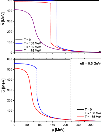
Figure 1: Behavior of $\bar{\sigma}$ as a function of $\mu$ for different values of the temperature and the magnetic field.

As is well known, the chiral quark-antiquark condensates are appropriate order parameters for the chiral symmetry restoration transition. In Fig. 2 we show the behavior of the averaged chiral condensate as a function of the external magnetic field, for some representative values of both $T$ and $\mu$. The numerical results correspond to parametrization P230. In all three panels it is seen that for $T=0$ the condensates show a monotonic increase with $B$, i.e. one has magnetic catalysis. On the contrary, when the temperature is increased, for $\mu=0$ the curves become non-monotonic, showing inverse magnetic catalysis. This is also reflected in the fact that the chiral restoration critical temperature gets reduced when the magnetic field is increased Dumm et al. (2017). Now, for values of the quark chemical potential beyond $\sim 100$ MeV (see central and lower panels of Fig. 2) the system enters the first order transition region, and the curves show discontinuities at some critical values of the magnetic field.

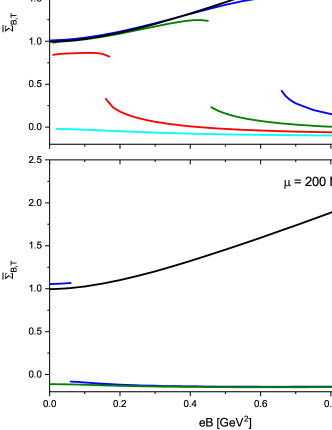
Figure 2: Flavor-averaged chiral condensate as a function of $eB$ for different representative values of the temperature and the quark chemical potential.

To specify the critical temperatures for the crossover transitions we take into account the maxima of the chiral susceptibility, defined as $\chi_{\rm ch}=-\partial[(\langle{\bar{u}u}\rangle_{B,T,\mu}^{\rm reg}+\langle{\bar{d}d}\rangle_{B,T,\mu}^{\rm reg})/2]/\partial T$. On the other hand, as stated, for the deconfinement we take the Polyakov loop as the relevant order parameter; therefore, to characterize the crossover-like transitions we consider the PL susceptibility, which is defined as $\chi_{\Phi}=\partial\Phi/\partial T$. It is seen that in the region where both chiral restoration and deconfinement transitions proceed as smooth crossovers, the peaks of the corresponding susceptibilities occur at approximately the same temperatures and chemical potentials (i.e., both transitions take place simultaneously).

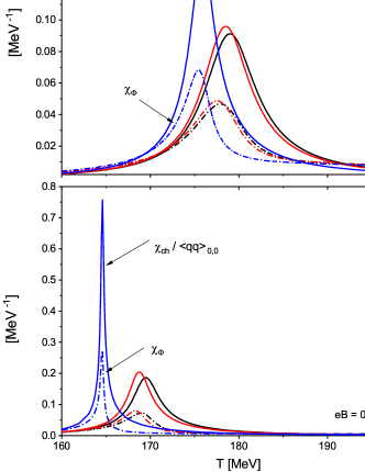
Figure 3: Behavior of the chiral and PL susceptibilities as a function of temperature for $eB=0$ and $eB=0.5$ GeV².

This is shown in Fig. 3, where we show the behavior of $\chi_{\rm ch}$ and $\chi_{\Phi}$ for two different magnetic field strengths and some representative values of the chemical potential corresponding to the crossover region. As already mentioned, we see that the peaks in $\chi_{\rm ch}$ and $\chi_{\Phi}$ are practically overlapped in the whole crossover region, i.e. the both crossover transitions are found to occur simultaneously.

It is also interesting to analyze the behavior of the critical chiral restoration temperature for different sets of model parameters. In the upper panel of Fig. 4 we show the critical temperature at $\mu=0$ as a function of the parameter set, which we characterize by the value of the $T=0$ chiral quark-antiquark condensate. We illustrate the situation by considering three representative values of the external magnetic field. In the figure, solid and dashed lines correspond to first-order and crossover-like transition regions, respectively. Let us consider firstly the $B=0$ case. It is seen that for parameter sets leading to condensate values $-\langle\bar{q}q\rangle^{1/3}\lesssim 220$ MeV the transition is predicted to be of first order, in contradiction with LQCD calculations; on the other hand, for larger condensates one finds crossover-like transitions at a stable critical temperature of about 175 to 180 MeV, in reasonable agreement with LQCD results. Going to the case of nonzero external magnetic field, the blue and red lines correspond to $eB=0.5$ and $eB=1$ GeV², respectively. It can be seen that for parametrizations leading to condensate values up to 250 MeV the critical temperatures get reduced when the magnetic field is increased, i.e. one observes the IMC effect; for larger condensates, instead, the critical temperature reaches a maximum at some value of $eB$. These behaviors are shown in the lower panel of Fig. 4, where we display the critical temperatures —normalized to the corresponding values at vanishing external magnetic field— as functions of $eB$, for different parametrizations. For P200 (solid line), one has a first order transition for all values of the magnetic field. For P230 the transition is crossover-like, and one has IMC; moreover, in this case the critical temperatures are found to be compatible with the results from LQCD quoted in Ref. Bali et al. (2012b), indicated by the gray band. Notice that LQCD calculations correspond to a three-flavor model; however, the normalized values of the critical temperatures are not expected to be significantly affected by the inclusion of strangeness. In the case of P260 the IMC effect is reduced (in fact, the critical temperature reaches a maximum for $eB\simeq 0.1$ GeV²) and gets progressively lost for parametrizations leading to larger values of the chiral condensate. In view of these results we take P230 as our preferred parametrization throughout this work.

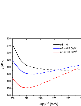
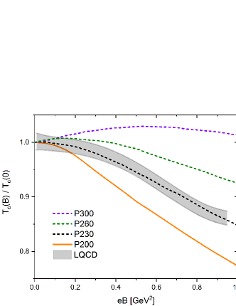
Figure 4: Upper panel: chiral critical temperatures $T_{c}$ at $\mu=0$ as functions of the predicted value for the chiral quark condensate $-\langle qq\rangle^{1/3}$, for different values of $eB$. Lower panel: Normalized critical temperatures as functions of $eB$ for various model parametrizations. Solid (dashed) lines correspond to first order (crossover) transitions. For comparison, three-flavor LQCD results from Ref. Bali et al. (2012b) are indicated by the gray band.

Next, in Fig. 5 we plot the critical temperature as a function of the magnetic field, for some representative values of the quark chemical potential. Starting from the curve for $\mu=0$ (black dashed line, corresponding to the black dashed line in the lower panel of Fig. 4), it is seen that the IMC effect is preserved for nonzero values of $\mu$. As expected, for relatively large values of $\mu$ the curves reach the $T=0$ axis, since chiral symmetry is approximately restored even at vanishing temperature (in absence of the external magnetic field one has $\mu_{c}(T=0)\simeq 340$ MeV; no chiral symmetry broken phase exists for values of $\mu$ beyond this limit (Ferraris et al., 2021)). Once again, solid (dashed) lines correspond to first order (crossover-like) transitions. While for $\mu=0$ it is seen that the transition is smooth for all values of $eB$, it becomes of first order for large values of $\mu$. In the case of the curve corresponding to $\mu=90$ MeV (green line), we find a first order piece for intermediate magnetic fields, viz. $0.3\lesssim eB\lesssim 0.9$. This is a manifestation of the particular behavior of the position of CEP, and can be clearly seen from the $\mu-T$ phase diagram (see Fig. 6).

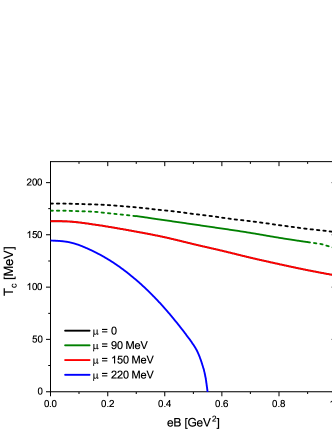
Figure 5: Chiral restoration critical temperature as a function of $eB$ for some representative values of the quark chemical potential.

In Fig. 6 we show the phase diagram in the $\mu-T$ plane, taking into account some values of the magnetic field to cover the range $eB=0$ to 1 GeV². As a general feature, it is seen that the pattern of a first order transition line (solid) and a crossover transition line (dashed) that meet at a critical end point is maintained for the considered range of values of the magnetic field. As stated, the dashed lines correspond both to the chiral restoration and the deconfinement transitions, which are found to be strongly correlated. In addition, it is seen that crossover transition lines get approximately overlapped for low magnetic fields ($0\leq eB\lesssim 0.1$ GeV²). It is worth looking at the location $(\mu_{\rm CEP},T_{\rm CEP})$ of the critical end point for the studied magnetic field range; the corresponding values are indicated in the figure by the wide gray line. It is found that the temperature $T_{\rm CEP}$ decreases steadily with the magnetic field, while the chemical potential $\mu_{\rm CEP}$ lies between about 80 to 105 MeV, reaching its minimum for intermediate values of the magnetic field. This behavior is remarkably different from the one obtained in Refs. (Avancini et al., 2012; Ferrari et al., 2012) in the framework of 2- and 3-flavor local NJL-like models, where the CEP temperature is found to grow when the external magnetic field get increased. Our results also differ qualitatively from those obtained in Ref. (Costa et al., 2015), where the authors consider a PNJL model in which the IMC effect is reproduced by including a $B$-dependent four-quark coupling.

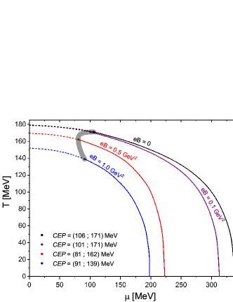
Figure 6: Phase diagram in $\mu-T$ plane for different values of $eB$. Solid and dashed lines correspond to first order and crossover transitions, respectively. The gray band indicates the locations of the critical end points.

Finally, for completeness we show in Fig. 7 the phase diagram in the $\mu-eB$ plane, considering several representative values of the temperature. The curve for $T=0$, previously obtained in Ref. Ferraris et al. (2021), shows that the critical chemical potential is a decreasing function of the magnetic field, and the transition is of first order for the considered range of values of $B$. We see from the figure that this decreasing behavior is maintained for larger values of $T$, while the curves reach the CEPs (indicated by the wide gray line) at $B<1$ GeV² for temperatures below $\simeq 140$ MeV. For values of $T$ between $\simeq 170$ and 180 MeV only crossover transitions can occur, whereas (as one can see from Fig. 6) no chiral symmetry broken phase exists for temperatures above $T_{c}(B=0)=180$ MeV.

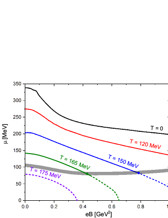
Figure 7: Phase diagram in $\mu-eB$ plane for different temperatures. Solid and dashed lines represent first-order and crossover transitions, respectively. The gray band indicates the locations of the critical end points.

IV Summary and conclusions

We have studied the QCD phase diagram, for both nonzero temperature and chemical potential, in the presence of an external static and uniform magnetic field. Our analysis has been done in the framework of a two-flavor nonlocal version of the NJL model, including the couplings of fermions to the Polyakov loop. This model has the feature of offering a natural mechanism for the description of the IMC effect observed through LQCD calculations.

Our numerical analysis shows that the IMC, reflected by a decreasing behavior of the critical chiral transition temperature as a function of the magnetic field, is preserved for nonzero values of the chemical potential. In addition, the qualitative features of the transition curves known for $B=0$ —consisting in a crossover region and a first order transition line, separated by a critical end point— is maintained for values of $eB$ ranging from zero to 1 GeV². From the analysis of the behavior of the traced Polyakov loop, it is seen that in the crossover region chiral restoration and deconfinement transitions occur simultaneously, in agreement with LQCD predictions. Moreover, it is found that the CEP exists for the whole considered range of the magnetic field, in a region that could be accessible for relativistic heavy ion collision experiments.

Our results for the location $(\mu_{\rm CEP},T_{\rm CEP})$ of the critical end point show that the chemical potential $\mu_{\rm CEP}$ lies in a relatively narrow region, between say 80 and 105 MeV, reaching the minimum for an intermediate value of the magnetic field, $eB\simeq 0.5$ GeV². On the other hand, the temperature $T_{\rm CEP}$ is found to decrease monotonously with the magnetic field, from $T_{\rm CEP}\simeq 170$ MeV for $eB=0$ to $T_{\rm CEP}\simeq 140$ MeV for $eB\simeq 1$ GeV². This behavior is opposite to the one observed in most studies of local versions of the NJL/PNJL models, in which $T_{\rm CEP}$ gets enhanced for increasing values of the magnetic field (Avancini et al., 2012; Ferrari et al., 2012; Costa et al., 2014, 2015; Ferreira et al., 2018a). We find it natural to attribute this qualitative difference to the fact that the nonlocal PNJL has the feature of showing IMC at vanishing chemical potential; as stated, the decrease of the critical temperature with the magnetic field also occurs at finite $\mu$, leading to the descent of the temperature of the CEP. In fact, in the local NJL model it is also found that the behavior of $T_{\rm CEP}$ with the magnetic field is significantly modified if one considers a $B$-dependent effective quark coupling such that the model could show IMC (Costa et al., 2015). It is also worth mentioning that although our results have been obtained for a two-flavor model, the values of $\mu_{\rm CEP}$ remain well below the $s$ quark threshold, and we have verified that the IMC observed at finite $\mu$ is robust under moderate changes in the model parameters; hence, the behavior of the CEP we have found in the low density region should not be qualitatively modified by the inclusion of strangeness degrees of freedom (notice that a more complex structure, including other CEPs, could be found at higher densities Ferreira et al. (2018a)). In this way, although it is still difficult to get definite predictions about the CEP location, it is seen that its behavior as a function of the magnetic field can be taken as an important clue to get insight on the character of effective four-point quark interactions and the effect of inverse magnetic catalysis.