A note on the boundary stabilization of the KdV-KdV system with time-dependent delay

Abstract.

The boundary stabilization problem of the Boussinesq KdV-KdV type system is investigated in this note. An appropriate boundary feedback law consisting of a linear combination of a damping mechanism and a time-varying delay term is designed. Then, under a small restriction on the length of the spatial domain and the initial data, we show that the energy of the KdV-KdV system decays exponentially.

1. Introduction

1.1. Boussinesq system model

The Boussinesq system is a set of partial differential equations that describes the behavior of waves in fluids with small-amplitude and long-wavelength disturbances. It was first introduced by the French mathematician Joseph Boussinesq in the 19th century as a way to model waves in shallow water [6]. Since then, the system has been used to study a wide range of physical phenomena, including ocean currents, atmospheric circulation, and heat transfer in fluids. The Boussinesq system is also an important tool in the study of fluid dynamics and has applications in a variety of fields, including meteorology, oceanography, and engineering.

Recently, Bona et al. in [3, 4] developed a four-parameter family of Boussinesq systems to describe the motion of small-amplitude long waves on the surface of an ideal fluid under gravity and in situations where the motion is sensibly two-dimensional. They specifically investigated a family of systems of the form

(1.1) $$\begin{cases}\eta_{t}(t,x)+\omega_{x}(t,x)+a\omega_{xxx}(t,x)-b\eta_{xxt}(t,x)+(\eta(t,x)\omega(t,x))_{x}=0,\\ \omega_{t}(t,x)+\eta_{x}(t,x)+c\eta_{xxx}(t,x)-d\omega_{xxt}(t,x)+\omega(t,x)\omega_{x}(t,x)=0,\end{cases}$$

which are all Euler equation approximations of the same order. Here $\eta$ represents the elevation of the equilibrium point and $\omega=\omega_{\theta}$ is the horizontal velocity in the flow at height $\theta\ell$, where $\theta\in[0,1]$ and $\ell$ is the undisturbed depth of the fluid. The parameters $a,b,c,d$, that one might choose in a given modeling situation, are required to fulfill the relations $a+b=\frac{1}{2}\left(\theta^{2}-\frac{1}{3}\right)$ and $c+d=\frac{1}{2}(1-\theta^{2})\geq 0.$

When $b=d=0$ and making a scaling argument, we obtain the Boussinesq system of KdV-KdV type

(1.2) $$\begin{cases}\eta_{t}(t,x)+\omega_{x}(t,x)+\omega_{xxx}(t,x)+(\eta(t,x)\omega(t,x))_{x}=0,\\ \omega_{t}(t,x)+\eta_{x}(t,x)+\eta_{xxx}(t,x)+\omega(t,x)\omega_{x}(t,x)=0,\end{cases}$$

which is shown to admit global solutions on $\mathbb{R}$ and it also has good control properties such as stabilization, and controllability, in periodic framework $\mathbb{T}$. However, stabilization properties for the Boussinesq KdV-KdV system on a bounded domain of $\mathbb{R}$ is a challenging problem due to the coupling of the nonlinear and dispersive nature of the equations. In this spirit, a few works indicate that appropriate boundary feedback conditions provide good stabilization results to the system (1.7) on a bounded domain $\mathbb{R}$ (see, for instance, [8, 9, 13, 21]).

1.2. Problem setting

In the sequel, consider the KdV-KdV equation (1.2) but in a bounded domain $[0,L]$ and with the following set of boundary conditions

(1.3) $$\begin{cases}\eta(t,0)=\eta(t,L)=\eta_{x}(t,0)=0,&t\in\mathbb{R}^{+},\\ \omega(t,0)=\omega(t,L)=\omega_{x}(t,L)=0,&t\in\mathbb{R}^{+}.\end{cases}$$

As mentioned before, note that considering the system described above, two important facts need to be mentioned:

$\bullet$ We first notice that the global Kato smoothing effect does not hold for the set of boundary condition (1.3). This makes impossible the task of showing the well-posedness findings employing classical methods, such as semigroup theory, and hence the well-posedness problem of this system remains open.

$\bullet$ The second issue is related to the energy of the system (1.2) and (1.3). Under the above boundary conditions, a simple integration by parts yields

$$\frac{d}{dt}E_{0}(t)=-\int_{0}^{L}(\eta(t,x)\omega(t,x))_{x}\eta(t,x)\,dx,$$

where

$$E_{0}(t)=\frac{1}{2}\int_{0}^{L}(\eta^{2}(t,x)+\omega^{2}(t,x))\,dx$$

is the total energy associated to (1.2) and (1.3). This indicates that we do not have any control over the energy in the sense that its time-derivative does have a fixed sign.

Therefore, due to the restriction presented in these two points, the following questions naturally arise:

Question $\mathcal{A}$: Is there a suitable set of boundary conditions so that the Kato smoothing effect can be revealed?

Question $\mathcal{B}$: Is there a feedback control law that permits to control of the nonlinear term presented in the derivative of the energy associated with the closed-loop system? Moreover, is this desired feedback law strong enough in the presence of a time-delay?

Question $\mathcal{C}$: If the answer to these previous questions is yes, does $E_{0}(t)\to 0$ as $t\to\infty$? If it is the case, can we give an explicit decay rate?

Our motivation in this work is to give answers to these questions. In this spirit, to deal with the Boussinesq system of KdV-KdV type (1.2), consider the set of boundary conditions

(1.4) $$\begin{cases}\eta(t,0)=\eta(t,L)=\eta_{x}(t,0)=\omega(t,0)=\omega(t,L)=0,&t>0,\\ \omega_{x}(t,L)=-\alpha\eta_{x}(t,L)+\beta\eta_{x}(t-\tau(t),L),&t>0,\end{cases}$$

where $\tau(t)$ is the time-varying delay. Here $\alpha$ and $\beta$ must satisfy the constraint

(1.5) $$\alpha>0,\quad(2\alpha-\lvert\beta\rvert)(1-d)>\lvert\beta\rvert,\quad\text{for $0\leq d<1$}.$$

Remark 1.

The following remarks are now in order.

• Note that our new set of boundary conditions contains a damping mechanism $\alpha\eta_{x}(t,L)$ as well as the time-varying delayed feedback $\beta\eta_{x}(t-\tau(t),L)$.

• The damping mechanism will guarantee the Kato smoothing effect, which is paramount to proving the well-posedness of the system under consideration in this article.

• The time-varying delay feedback, together with the damping mechanism, permits to drive of the energy to $0$ as $t$ goes to $\infty$, giving the stabilization of the system (1.2) and (1.4) with precise decay rate.

It is also noteworthy that time delay phenomena occur in numerous areas, including biology, mechanics, and engineering. In the context of dispersive equations, time-delayed feedback is a challenging problem because it can lead to instability or oscillatory behavior in numerous systems. Some recent results - not exhaustive - already addressed the stabilization problem of dispersive systems. We can cite, for example, [2], [14] and [7] for KdV, KS, and Kawahara equations, where time-delay boundary controls are considered. Furthermore, if the time-delayed occurs in the equation, the authors in [24], [11, 15], and [12] showed stabilization results for the KdV, fifth-order KdV, and KP-II equations, respectively. Finally, note that using the time-varying delay, the authors in [18] and [20] obtained stabilization outcomes for the wave and KdV equations, respectively. The reader is referred to these papers and the references therein for more details about this topic.

1.3. Main result and paper’s outline

To our knowledge, due to the previous restrictions, there is no result combining the damping mechanism and the boundary time-varying delay to guarantee stabilization results for the KdV-KdV system (1.2) and (1.4). To give the first result in this direction, and provide answers to the questions previously mentioned, let us assume that there exist two positive constants $M$ and $d<1$ such that the time-dependent function $\tau(t)$ satisfies the following standard conditions:

(1.6) $$\begin{cases}0<\tau(0)\leq\tau(t)\leq M,\quad\dot{\tau}(t)\leq d<1,&\forall t\geq 0,\\ \tau\in W^{2,\infty}([0,T]),&T>0.\end{cases}$$

Next, let $X_{0}:=L^{2}(0,L)\times L^{2}(0,L),$ $H:=X_{0}\times L^{2}(0,1)$ and consider in

$$\mathcal{B}:=C([0,T],X_{0})\cap L^{2}(0,T,[H^{1}(0,L)]^{2})$$

the norm $\lVert(\eta,\omega)\rVert_{\mathcal{B}}=\sup_{t\in[0,T]}\lVert(\eta(t),\omega(t))\rVert_{X_{0}}+\lVert(\eta_{x},\omega_{x})\rVert_{L^{2}(0,T;X_{0})}.$ Whereupon, we are interested in the behavior of the solutions of the system

(1.7) $$\begin{cases}\eta_{t}(t,x)+\omega_{x}(t,x)+\omega_{xxx}(t,x)+(\eta(t,x)\omega(t,x))_{x}=0,&\mathbb{R}^{+}\times(0,L),\\ \omega_{t}(t,x)+\eta_{x}(t,x)+\eta_{xxx}(t,x)+\omega(t,x)\omega_{x}(t,x)=0,&\mathbb{R}^{+}\times(0,L),\\ \eta_{x}(t-\tau(0),L)=z_{0}(t-\tau(0))\in L^{2}(0,1),&0<t<\tau(0),\\ \left(\eta(0,x),\omega(0,x)\right)=\left(\eta_{0}(x),\omega_{0}(x)\right)\in X_{0},&x\in(0,L).\end{cases}$$

with boundary condition (1.4). Note that the total energy associated with the system (1.7) will be defined in $H$ by

(1.8) $$E(t)=\frac{1}{2}\int_{0}^{L}(\eta^{2}(t,x)+\omega^{2}(t,x))\,dx+\frac{\lvert\beta\rvert}{2}\tau(t)\int_{0}^{1}\eta_{x}^{2}(t-\tau(t)\rho,L)\,d\rho.$$

Thereafter, the principal result of the article ensures that the energy $E(t)$ decays exponentially despite the presence of the delay. An estimate of the decay rate is also provided. This answers each question that we tabled previously.

Theorem 1.1.

Let $0<L<\sqrt{3}\pi$. Suppose that (1.5) and (1.6) are satisfied. Then, for two constants $\mu_{1}$ and $\mu_{2}$ small enough, there exist

(1.9) $$0<r<\frac{\mu_{1}(3\pi^{2}-L^{2})}{2\pi^{2}L^{\frac{1}{2}}(2L+1)},\quad\kappa\leq 1+\max\{2\mu_{1}L,\mu_{2}\},$$

and

(1.10) $$\lambda\leq\min\left\{\frac{\mu_{1}\left(3\pi^{2}-L^{2}\right)-2r\pi^{2}L^{\frac{1}{2}}(2L+1)}{L^{2}(1+2\mu_{1}L)},\frac{\mu_{2}(1-d)}{M(1+\mu_{2})}\right\}$$

such that the the total energy $E(t)$ given by (1.8) satisfies

$$E(t)\leq\kappa E(0)e^{-\lambda t},$$

for all $t>0$, provided that the initial data of the solution $(\eta,w)$ of (1.7)-(1.4) obeys $\lVert(\eta_{0},\omega_{0};z_{0}(\cdot-\tau(0)))\rVert_{H}\leq r$.

This paper consists of four parts including the Introduction. Section 2 discusses the existence of solutions for the nonlinear Boussinesq KdV-KdV system (1.7). Section 3 is devoted to proving the stabilization result, namely, Theorem 1.1. Finally, in Section 4, we will provide some concluding remarks and discuss open problems related to the stabilization of the nonlinear Boussinesq KdV-KdV system (1.7).

2. Well-posedness theory

2.1. Linear problem

Consider the following linear Cauchy problem

(2.1) $$\begin{split}\dfrac{d}{dt}U(t)=A(t)U(t),\quad U(0)=U_{0},&\quad t>0,\end{split}$$

where $A(t)\colon D(A(t))\subset{H}\to{H}$ is densely defined. If $D(A(t))$ is independent of time $t$, i.e., $D(A(t))=D(A(0)),$ for $t>0.$ The next theorem ensures the existence and uniqueness of the Cauchy problem (2.1).

Theorem 2.1 ([22]).

Assume that:

1. $\mathcal{Z}=D(A(0))$ is a dense subset of $H$ and $D(A(t))=D(A(0))$, for all $t>0$,

2. $A(t)$ generates a strongly continuous semigroup on $H$. Moreover, the family $\{A(t)\colon t\in[0,T]\}$ is stable with stability constants $C,\ m$ independent of $t$.

3. $\partial_{t}A(t)$ belongs to $L_{\ast}^{\infty}([0,T],B(\mathcal{Z},H))$, the space of equivalent classes of essentially bounded, strongly measure functions from $[0,T]$ into the set $B(\mathcal{Z},H)$ of bounded operators from $\mathcal{Z}$ into $H$.

Then, problem (2.1) has a unique solution $U\in C([0,T],\mathcal{Z})\cap C^{1}([0,T],H)$ for any initial data in $\mathcal{Z}$.

The task ahead is to apply the above result to ensure the existence of solutions for the linear system associated with (1.7). To do that, consider the following linearized system associated with (1.7), that is, consider the equation without $\omega(t,x)\omega_{x}(t,x)$ and $(\eta(t,x)\omega(t,x))_{x}$. Following the ideas introduced by in [17], let us define the auxiliary variable $z(t,\rho)=\eta_{x}(t-\tau(t)\rho,L)$, which satisfies the transport equation:

(2.2) $$\begin{cases}\tau(t)z_{t}(t,\rho)+(1-\dot{\tau}(t)\rho)z_{\rho}(t,\rho)=0,&t>0,\rho\in(0,1),\\ z(t,0)=\eta_{x}(t,L),\ z(0,\rho)=z_{0}(-\tau(0)\rho)&t>0,\ \rho\in(0,1).\end{cases}$$

Now, the space $H$ will be equipped with the inner product

(2.3) $$\left\langle\left(\eta,\omega,z\right),\left(\tilde{\eta},\tilde{\omega},\tilde{z}\right)\right\rangle_{t}= \left\langle\left(\eta,\omega\right),\left(\tilde{\eta},\tilde{\omega}\right)\right\rangle_{X_{0}}+\lvert\beta\rvert\tau(t)\left\langle z,\tilde{z}\right\rangle_{L^{2}(0,1)},$$

for any $(\eta,\omega;z),(\tilde{\eta},\tilde{\omega};\tilde{z})\in H$.

Now, picking $U=(\eta,\omega;z)^{T}$ and $A(t)\colon D(A(t))\subset{H}\to{H}$ given by

(2.4) $$A(t)\left(\eta,\omega,z\right):=\left(-\omega_{x}-\omega_{xxx},-\eta_{x}-\eta_{xxx},\dfrac{\dot{\tau}(t)\rho-1}{\tau(t)}z_{\rho}\right)$$

with domain defined by

(2.5) $$D(A(t))=\left\{\begin{aligned} (\eta,\omega)&\in\left[H^{3}(0,L)\cap H_{0}^{1}(0,L)\right]^{2}\\ z&\in H^{1}(0,1)\end{aligned}\left\lvert\begin{aligned} &\eta_{x}(0)=0,z(0)=\eta_{x}(L),\\ &\omega_{x}(L)=-\alpha\eta_{x}(L)+\beta z(1).\end{aligned}\right.\right\},$$

we rewrite (2.2)-(2.5) as an abstract Cauchy problem (2.1). Moreover, note that $D(A(t))$ is independent of time $t$ and satisfies $D(A(t))=D(A(0))$. Consider the triplet $\{A,H,\mathcal{Z}\}$, with $A=\left\{A(t)\colon t\in[0,T]\right\}$ for some $T>0$ fixed and $\mathcal{Z}=D(A(0))$. Now, we can prove a well-posedness result of (2.1) related to $\{A,H,\mathcal{Z}\}$.

Theorem 2.2.

Assume that $\alpha$ and $\beta$ are real constants such that (1.5) holds. Taking $U_{0}\in H$, there exists a unique solution $U\in C([0,+\infty),H)$ to (2.1). Moreover, if $U_{0}\in D(A(0))$, then $U\in C([0,+\infty),D(A(0)))\cap C^{1}([0,+\infty),H).$

Proof.

The result will be proved classically (see, for instance, [18]). First, it is not difficult to see that $\mathcal{Z}=D(A(0))$ is a dense subset of $H$ and $D(A(t))=D(A(0))$, for all $t>0$. Therefore, item (1) of Theorem 2.1 holds.

For item (2) of Theorem 2.1, note that integrating by parts and using the boundary conditions, we have that

$$\left\langle A(t)U,U\right\rangle_{t}-\kappa(t)\left\langle U,U\right\rangle_{t}\leq\frac{1}{2}\left(\eta_{x}(L)\ \ \eta_{x}(t-\tau(t),L)\right)\Phi_{\alpha,\beta}\left(\eta_{x}(L)\ \ \eta_{x}(t-\tau(t),L)\right)^{T}$$

where

$$\kappa(t)=\frac{(\dot{\tau}(t)^{2}+1)^{\frac{1}{2}}}{2\tau(t)}\quad\text{and}\quad\Phi_{\alpha,\beta}=\begin{pmatrix}-2\alpha+\lvert\beta\rvert&\beta\\ \beta&\lvert\beta\rvert(d-1)\end{pmatrix}.$$

Invoking (1.5), we deduce that $\Phi_{\alpha,\beta}$ is a negative definite matrix and consequently we get $\left\langle A(t)U,U\right\rangle_{t}-\kappa(t)\left\langle U,U\right\rangle_{t}\leq 0.$ Thereby, $\tilde{A}(t)=A(t)-\kappa(t)I$ is dissipative.

On the other hand, we claim the following:

Claim 1.

For all $t\in[0,T]$, the operator $A(t)$ is maximal, or equivalently, for some $\lambda>0$ we have that $\lambda I-A(t)$ is surjective.

In fact, let $t\in[0,T]$ fixed, $(f_{1},f_{2},h)^{T}\in H$, and consider $U=(\eta,\omega,z)^{T}\in D(A(t))$ solution of

(2.6) $$(\lambda I-A(t))U=(f_{1},f_{2},h)\iff\begin{cases}\lambda\eta+\omega_{x}+\omega_{xxx}=f_{1},\\ \lambda\omega+\eta_{x}+\eta_{xxx}=f_{2},\\ \lambda z+\left(\dfrac{1-\dot{\tau}(t)\rho}{\tau(t)}\right)z_{\rho}=h,\end{cases}$$

satisfying (2.5). Note that $z$ has the explicit form

$$z(\rho)=\begin{cases}\displaystyle\eta_{x}(L)e^{-\lambda\tau(t)\rho}+\displaystyle\tau(t)e^{-\lambda\tau(t)\rho}\int_{0}^{\rho}e^{\lambda\tau(t)\sigma}h(\sigma)\,d\sigma,&\!\!\!\text{if }\dot{\tau}(t)=0,\\[2.84526pt] \displaystyle e^{\lambda\frac{\tau(t)}{\dot{\tau}(t)}\ln(1-\dot{\tau}(t)\rho)}\left[\eta_{x}(L)\displaystyle+\int_{0}^{\rho}\frac{h(\sigma)\tau(t)}{1-\dot{\tau}(t)\sigma}e^{-\lambda\frac{\tau(t)}{\dot{\tau}(t)}\ln(1-\dot{\tau}(t)\sigma)}\,d\sigma\right],&\!\!\!\text{if }\dot{\tau}(t)\neq 0.\end{cases}$$

In particular, $z(1)=\eta_{x}(L)g_{0}(t)+g_{h}(t)$, where

$$g_{0}(t)=\begin{cases}\displaystyle e^{-\lambda\tau(t)},&\text{ if }\dot{\tau}(t)=0,\\ \displaystyle e^{\lambda\frac{\tau(t)}{\dot{\tau}(t)}\ln(1-\dot{\tau}(t))},&\text{ if }\dot{\tau}(t)\neq 0,\end{cases}$$

and

$$g_{h}(t)=\begin{cases}\displaystyle\tau(t)e^{-\lambda\tau(t)}\int_{0}^{1}e^{\lambda\tau(t)\sigma}h(\sigma)d\sigma,&\text{ if }\dot{\tau}(t)=0,\\ \displaystyle e^{\lambda\frac{\tau(t)}{\dot{\tau}(t)}\ln(1-\dot{\tau}(t))}\int_{0}^{1}\frac{h(\sigma)\tau(t)}{1-\dot{\tau}(t)\sigma}e^{-\lambda\frac{\tau(t)}{\dot{\tau}(t)}\ln(1-\dot{\tau}(t)\sigma)}d\sigma,&\text{ if }\dot{\tau}(t)\neq 0.\end{cases}$$

Thus, $\eta,\omega$ should satisfy

(2.7) $$\begin{cases}\lambda\eta+\omega_{x}+\omega_{xxx}=f_{1},\\ \lambda\omega+\eta_{x}+\eta_{xxx}=f_{2},\end{cases}$$

with boundary condition

(2.8) $$\begin{cases}\eta(0)=\eta(L)=\omega(0)=\omega(L)=\eta_{x}(0)=0,\\ \omega_{x}(L)=(-\alpha+\beta g_{0}(t))\eta_{x}(L)+\beta g_{h}(t).\end{cases}$$

Pick $\psi(x,t)=\dfrac{x(x-L)}{L}\beta g_{h}(t)\in C^{\infty}([0,L])$ and let $\hat{\omega}:=\omega-\psi$. Then, the system (2.7) can be rewritten as follows:

(2.9) $$\begin{cases}\lambda\eta+\omega_{x}+\omega_{xxx}=f_{1}-\psi_{x}=:\tilde{f_{1}},\\ \lambda\omega+\eta_{x}+\eta_{xxx}=f_{2}-\lambda\psi=:\tilde{f_{2}},\end{cases}$$

and satisfies (2.8). Note that for the sake of the presentation clarity, we still use $\omega$ after translation. One can check that $0<g_{0}(t)<1$ and hence $-\tilde{\alpha}:=-\alpha+\beta g_{0}(t)<0$, thanks to (1.5). Thus, our Claim 1 is reduced to proving that $\lambda I-\hat{A}$ is surjective with $\hat{A}$ given by $\hat{A}(\eta,\omega)=(-\omega_{x}-\omega_{xxx},-\eta_{x}-\eta_{xxx})$ with dense domain

$$D(\hat{A}):=\left\{(\eta,\omega)\in\left[H^{3}(0,L)\cap H_{0}^{1}(0,L)\right]^{2}\colon\eta_{x}(0)=0,\ \omega_{x}(L)=-\tilde{\alpha}\eta_{x}(L)\right\}\subset X_{0}.$$

Thanks to [13, Proposition 4.1], the operators $\hat{A}$ and $\hat{A}^{\ast}$ are dissipative, and the desired result follows by Lummer-Phillips Theorem (see, for example, [19]). This shows the Claim 1. Consequently, $\tilde{A}(t)$ generates a strongly semigroup on $H$ and $\tilde{A}=\{\tilde{A}(t),t\in[0,T]\}$ is a stable family of generators in $H$ with a stability constant independent of $t$, and the item (2) of Theorem 2.1 is satisfied.

Finally, due to the fact that $\tau\in W^{2,\infty}([0,T])$ for all $T>0$, we have

$$\dot{\kappa}(t)=\frac{\ddot{\tau}(t)\dot{\tau}(t)}{2\tau(t)\left(\dot{\tau}(t)^{2}+1\right)^{1/2}}-\frac{\dot{\tau}(t)\left(\dot{\tau}(t)^{2}+1\right)^{1/2}}{2\tau(t)^{2}}$$

is bounded on $[0,T]$ for all $T>0$. Moreover,

$$\frac{d}{dt}A(t)U=\left(0,0,\frac{\ddot{\tau}(t)\tau(t)\rho-\dot{\tau}(t)(\dot{\tau}(t)\rho-1)}{\tau(t)^{2}}z_{\rho}\right),$$

while the coefficient of $z_{\rho}$ is bounded on $[0,T]$ and the regularity of the item (3) of Theorem 2.1 is fulfilled.

Based on the above discussion, all the assumptions of Theorem 2.1 are verified. Therefore, for $U_{0}\in D({A}(0))$, the Cauchy problem

$$\begin{split}\tilde{U}_{t}(t)=\tilde{A}(t)\tilde{U}(t),\ \tilde{U}(0)=U_{0},&\quad t>0,\end{split}$$

has a unique solution $\tilde{U}\in C([0,\infty),H)$ and $\tilde{U}\in C([0,\infty),D({A}(0)))\cap C^{1}([0,\infty),H)$, and consequently the solution of (2.1) is $U(t)=e^{\int_{0}^{t}\kappa(s)ds}\tilde{U}(t)$. ∎

The next proposition states that the energy (1.8) is decreasing along the solutions of (2.1). The proof is straightforward and hence omitted.

Proposition 2.3.

Suppose $\alpha$ and $\beta$ are real constants such that (1.5) is satisfied. Then for any mild solution of (2.1) the energy $E(t)$ defined by (1.8) is non-increasing and

(2.10) $$\frac{d}{dt}E(t)=\frac{1}{2}\begin{pmatrix}\eta_{x}(L)\\ \eta_{x}(t-\tau(t),L)\end{pmatrix}^{T}\Phi_{\alpha,\beta}\begin{pmatrix}\eta_{x}(L)\\ \eta_{x}(t-\tau(t),L)\end{pmatrix}.$$

We finish this section by giving a priori estimates and the Kato smoothing effect which are essential to obtain the well-posedness of the system (1.7). Here, we consider $(S_{t}(s))_{s\geq 0}$ to be the semigroup of contractions associated to the operator $A(t)$.

Proposition 2.4.

Let $\alpha$ and $\beta$ are real constant such that (1.5) holds. Then, the map

$$(\eta_{0},\omega_{0};z_{0})\in{H}\mapsto(\eta,\omega;z)\in\mathcal{B}\times C(0,T;L^{2}(0,1))$$

is well-defined, continuous, and fulfills

(2.11) $$\lVert(\eta,\omega)\rVert_{X_{0}}^{2}+\lvert\beta\rvert\lVert z\rVert_{L^{2}(0,1)}^{2}\leq\lVert(\eta_{0},\omega_{0})\rVert_{X_{0}}^{2}+\lvert\beta\rvert\lVert z_{0}(-\tau(0)\cdot)\rVert_{L^{2}(0,1)}^{2},$$

Furthermore, for every $(\eta_{0},\omega_{0},z_{0})\in{H}$, we have that

(2.12) $$\lVert\eta_{x}(\cdot,L)\rVert_{L^{2}(0,T)}^{2}+\lVert z(\cdot,1)\rVert_{L^{2}(0,T)}^{2}\leq\lVert(\eta_{0},\omega_{0})\rVert_{X_{0}}^{2}+\lVert z_{0}(-\tau(0)\cdot)\rVert_{L^{2}(0,1)}^{2}.$$

Moreover, the Kato smoothing effect is verified

(2.13) $$\int_{0}^{T}\int_{0}^{L}\eta_{x}^{2}+\omega_{x}^{2}\,dx\,dt\leq C(L,T,\alpha)\left(\lVert(\eta_{0},\omega_{0})\rVert_{X_{0}}^{2}+\lVert z_{0}(-\tau(0)\cdot)\rVert_{L^{2}(0,1)}^{2}\right).$$

Finally, for the initial data, we have the following estimates

(2.14) $$\begin{split}\lVert(\eta_{0},\omega_{0})\rVert_{X_{0}}^{2}\leq&\frac{1}{T}\lVert(\eta,\omega)\rVert_{L^{2}(0,T;X_{0})}^{2}\\ &+(2\alpha+\lvert\beta\rvert)\lVert\eta_{x}(\cdot,L)\rVert_{L^{2}(0,T)}^{2}+\lvert\beta\rvert\lVert z(\cdot,1)\rVert_{L^{2}(0,1)}^{2}\end{split}$$

and

(2.15) $$\lVert z_{0}(-\tau(0)\cdot)\rVert_{L^{2}(0,1)}^{2}\leq C_{1}(d,M)\left(\lVert z(T,\cdot)\rVert_{L^{2}(0,1)}+\lVert z(\cdot,1)\rVert_{L^{2}(0,T)}^{2}\right).$$

Proof.

From (2.10) and using that $\Phi_{\alpha,\beta}$ is a symmetric definite negative matrix we obtain that $E^{\prime}(t)+\eta_{x}^{2}(t,L)+z^{2}(t,1)\leq 0$. Integrating in $[0,s]$, for $0\leq s\leq T$, we get

(2.16) $$E(s)+\int_{0}^{s}\eta_{x}^{2}(t,L)\,dt+\int_{0}^{s}z^{2}(t,1)\,dt\leq E(0),$$

and (2.11) is obtained. Taking $s=T$ and since $E(t)$ is a non-increasing function (see Proposition 2.3), the estimate (2.12) holds. Now, multiplying the first equation of the linearized system associated with (1.7) by $x\omega$ and the second one by $x\eta$ adding the results, integrating by parts in $(0,L)\times(0,T)$ and using (2.12), we obtain

(2.17) $$\frac{3}{2}\int_{0}^{T}\int_{0}^{L}\eta_{x}^{2}+\omega_{x}^{2}\,dx\,dt\leq(L+T)\lVert(\eta_{0},\omega_{0})\rVert_{X_{0}}^{2}$$

$$+\left(\alpha^{2}+\frac{1}{2}\right)L\left(\lVert\eta_{x}(\cdot,L)\rVert_{L^{2}(0,T)}^{2}+\lVert z(\cdot,1)\rVert_{L^{2}(0,T)}^{2}\right)$$

$$\leq C(L,T,\alpha)\left(\lVert(\eta_{0},\omega_{0})\rVert_{X_{0}}^{2}+\lVert z_{0}(-\tau(0)\cdot)\rVert_{L^{2}(0,1)}^{2}\right),$$

where $C(L,T,\alpha):=\max\left\{1,L+T,\left(\alpha^{2}+\frac{1}{2}\right)L\right\},$ showing (2.13). Secondly, multiplying the first equation of the linearized system associated with (1.7) by $(T-t)\eta$ and the second one by $(T-t)\omega$ adding the results, yields that

$$\begin{split}\frac{T}{2}\lVert(\eta_{0},\omega_{0})\rVert_{X_{0}}^{2}\leq&\frac{1}{2}\lVert(\eta,\omega)\rVert_{L^{2}(0,T,X_{0})}^{2}+T\left(\alpha+\frac{\lvert\beta\rvert}{2}\right)\int_{0}^{T}\eta_{x}^{2}(t,L)\,dt\\ &+T\frac{\lvert\beta\rvert}{2}\int_{0}^{T}z^{2}(t,1)\,dt,\end{split}$$

where we have used Young’s inequality, verifying (2.14). Finally, multiplying (2.2)₁ by $z$ and integrating by parts in $(0,T)\times(0,1)$,

$$\tau_{0}\int_{0}^{1}z_{0}^{2}(-\tau(0)\rho)\,d\rho\leq\int_{0}^{T}(1-\dot{\tau}(t))z^{2}(t,1)\,dt+\tau(T)\int_{0}^{1}z^{2}(T,\rho)\,d\rho,$$

giving (2.15). ∎

The next result ensures the solution for the KdV-KdV system with source terms.

Theorem 2.5.

Suppose that (1.5) and (1.6) holds. Let $U_{0}=(\eta_{0},\omega_{0},z_{0})\in H$ and the source terms $(f_{1},f_{2})\in L^{1}(0,T;X_{0})$. Then there exists a unique solution $U=(\eta,\omega,z)\in C([0,T],H)$ to

(2.18) $$\begin{cases}\eta_{t}(t,x)+\omega_{x}(t,x)+\omega_{xxx}(t,x)=f_{1},&t>0,x\in(0,L),\\ \omega_{t}(t,x)+\eta_{x}(t,x)+\eta_{xxx}(t,x)=f_{2},&t>0,x\in(0,L),\\ \eta(t,0)=\eta(t,L)=\eta_{x}(t,0)=\omega(t,0)=\omega(t,L)=0,&t>0,\end{cases}$$

with boundary condition as in (1.7). Moreover, for $T>0$, the following estimates hold

(2.19) $$\begin{cases}\begin{split}\lVert(\eta,\omega;z)\rVert_{C([0,T],H)}\leq C(\lVert(\eta_{0},\omega_{0},z_{0})\rVert_{H}+\lVert(f,g)\rVert_{L^{1}(0,T,X_{0})}),\\ \lVert(\eta_{x}(\cdot,L),z(\cdot,1))\rVert_{[L^{2}(0,T)]^{2}}^{2}\leq C(\lVert{(\eta_{0},\omega_{0},z_{0})}\rVert_{H}^{2}+\lVert(f,g)\rVert_{L^{1}(0,T,X_{0})}^{2})\\ \lVert(\eta,\omega)\rVert_{L^{2}([0,T],X_{1})}\leq C(\lVert(\eta_{0},\omega_{0},z_{0})\rVert_{H}+\lVert(f,g)\rVert_{L^{1}(0,T,X_{0})}),\end{split}\end{cases}$$

for some constant $C>0$.

Proof.

Similarly as done in the proof of Proposition 2.4, using (2.10) and taking into account that $\Phi_{\alpha,\beta}$ is a symmetric definite negative matrix, there exists $C>0$ such that $E^{\prime}(t)+\eta_{x}^{2}(t,L)+z^{2}(t,1)\leq C\left\langle(\eta,\omega),\ (f_{1},f_{2})\right\rangle_{X_{0}}.$ Integrating the previous inequality on $[0,s]$ for $0\leq s\leq T$, we get

(2.20) $$E(s)+\int_{0}^{s}\eta_{x}^{2}(t,L)\,dt+\int_{0}^{s}z^{2}(t,1)\,dt\leq C\left(\int_{0}^{s}\left\langle(\eta,\omega),(f_{1},f_{2})\right\rangle_{X_{0}}+E(0)\right).$$

From Cauchy-Schwarz inequality, follows that

$$\begin{split}\left\lVert(\eta(s,\cdot),\omega(s,\cdot);z(s,\cdot)\right\rVert_{H}^{2}\leq&C\left(\lVert(\eta_{0},\omega_{0};z_{0})\rVert_{H}^{2}\right.\\ &\left.+\lVert(f_{1},f_{2})\rvert_{L^{1}(0,T;X_{0})}\lVert(\eta,\omega)\rVert_{C([0,T],X_{0})}\right),\end{split}$$

therefore, taking the $\sup$-norm for $s\in[0,T]$ and applying Young’s inequality $\eqref{eq:APsou1}_{1}$ is obtained. Additionally, if we consider $s=T$ in (2.20), the estimate for the traces $\eqref{eq:APsou1}_{2}$ is guaranteed. Finally, by using the same Morawetz multipliers as in Proposition 2.4, we have

$$\int_{0}^{T}\int_{0}^{L}x\left(f_{1}\omega(t,x)+f_{2}\eta(t,x)\right)dxdt\leq L\lVert(\eta,\omega,z)\rVert_{C([0,T],H)}\lVert(f_{1},f_{2})\rVert_{L^{1}(0,T,X_{0})}$$

$$\leq C\left(\lVert(\eta_{0},\omega_{0};z_{0})\rVert_{H}^{2}+\lVert(f_{1},f_{2})\rVert_{L^{1}(0,T,X_{0})}^{2}\right),$$

proving $\eqref{eq:APsou1}_{3}$. ∎

2.2. Nonlinear problem

Using the theory for local well-posedness of nonlinear systems in [23], it amounts to proving that the map $\Gamma\colon\mathcal{B}\to\mathcal{B}$ has a unique fixed-point in some closed ball $B(0,R)\subset\mathcal{B}$ where $\Gamma(\tilde{\eta},\tilde{\omega})=(\eta,\omega)$ and $(\eta,\omega)$ are the solution of the system (1.7). The next result ensures that the nonlinear terms can be considered as a source term of the linear equation (2.18). The proof can be found in [13].

Proposition 2.6.

Let $(\eta,\omega)\in L^{2}(0,T,[H^{1}(0,L)]^{2})$, so $(\eta\omega)_{x}$, $\omega\omega_{x}\in L^{1}(0,T,X_{0})$ and $(\eta,\omega)\in\mathcal{B}\mapsto((\eta\omega)_{x},(\omega\omega_{x}))\in L^{1}(0,T,X_{0})$ is continuous. In addition, the following estimate holds,

$$\begin{split}\int_{0}^{T}\left\lVert((\eta_{1}\omega_{1})_{x}-(\eta_{2}\omega_{2})_{x},\omega_{1}\omega_{1,x}-\omega_{2}\omega_{2,x})\right\rVert_{X_{0}}dt\leq&KT^{\frac{1}{4}}\left(\lVert(\eta_{1},\omega_{1})\rVert_{\mathcal{B}}+\lVert(\eta_{2},\omega_{2})\rVert_{\mathcal{B}}\right)\\ &\times\lVert(\eta_{1}-\eta_{2},\omega_{1}-\omega_{2})\rVert_{\mathcal{B}}\,\end{split}$$

for a constant $K>0$.

Finally, let us present the existence of local solutions to (1.7).

Theorem 2.7.

Let $L,T>0$ and consider $\alpha$ and $\beta$ real constants such that (1.5) is satisfied. For each initial data $(\eta_{0},\omega_{0};z_{0})\in H$ sufficiently small, $\Gamma\colon\mathcal{B}\to\mathcal{B}$ defined by $\Gamma(\tilde{\eta},\tilde{\omega})=(\eta,\omega)$ is a contraction. Moreover, there exists a unique solution $(\eta,\omega)\in B(0,R)\subset\mathcal{B}$ of the Boussinesq KdV-KdV nonlinear system (1.7).

Proof.

It follows from Theorem 2.5 that the map $\Gamma$ is well defined. Using Proposition 2.6 and the a priori estimates we obtain

$$\lVert\Gamma(\tilde{\eta},\tilde{\omega})\rVert_{\mathcal{B}}=\lVert(\eta,\omega)\rVert_{\mathcal{B}}\leq C\left(\lVert(\eta_{0},\omega_{0},z_{0})\rVert_{H}+\lVert(\tilde{\eta},\tilde{\omega})\rVert_{\mathcal{B}}^{2}\right),$$

$$\left\lVert\Gamma(\tilde{\eta}_{1},\tilde{\omega}_{1})-\Gamma(\tilde{\eta}_{2},\tilde{\omega}_{2})\right\rVert_{\mathcal{B}}\leq KT^{\frac{1}{4}}\left(\lVert(\tilde{\eta}_{1},\tilde{\omega}_{1})\rVert_{\mathcal{B}}+\lVert(\tilde{\eta}_{2},\tilde{\omega}_{2})\rVert_{\mathcal{B}}\right)\lVert(\tilde{\eta}_{1}-\tilde{\eta}_{2},\tilde{\omega}_{1}-\tilde{\omega}_{2})\rVert_{\mathcal{B}}.$$

Now, we restrict $\Gamma$ to the closed ball $\{(\tilde{\eta},\tilde{\omega})\in\mathcal{B}:\lVert(\tilde{\eta},\tilde{\omega})\rVert_{\mathcal{B}}\leq R\}$, with $R>0$ to be determined later. Then, $\lVert\Gamma(\tilde{\eta},\tilde{\omega})\rVert_{\mathcal{B}}\leq C\left(\lVert(\eta_{0},\omega_{0},z_{0})\rVert_{H}+R^{2}\right)$ and

$$\left\lVert\Gamma(\tilde{\eta}_{1},\tilde{\omega}_{1})-\Gamma(\tilde{\eta}_{2},\tilde{\omega}_{2})\right\rVert_{\mathcal{B}}\leq 2RKT^{\frac{1}{4}}\lVert(\tilde{\eta}_{1}-\tilde{\eta}_{2},\tilde{\omega}_{1}-\tilde{\omega}_{2})\rVert_{\mathcal{B}}.$$

Next, we pick $R=2C\lVert(\eta_{0},\omega_{0},z_{0})\rVert_{H}$ and $T>0$ such that $2KT^{\frac{1}{4}}R<1$, with $C<2KT^{\frac{1}{4}}$. This leads to claim that

$$\lVert\Gamma(\tilde{\eta},\tilde{\omega})\rVert_{\mathcal{B}}\leq R$$

and

$$\left\lVert\Gamma(\tilde{\eta}_{1},\tilde{\omega}_{1})-\Gamma(\tilde{\eta}_{2},\tilde{\omega}_{2})\right\rVert_{\mathcal{B}}<C_{1}\lVert(\tilde{\eta}_{1}-\tilde{\eta}_{2},\tilde{\omega}_{1}-\tilde{\omega}_{2})\rVert_{\mathcal{B}}$$

, with $C_{1}<1$. Lastly, the result is an immediate consequence of the Banach fixed point theorem. ∎

Remark 2.

Note that the solutions of the system (1.7) obtained in Theorem 2.7 are global thanks to the Proposition 2.3.

3. Stabilization Result: Proof of Theorem 1.1

Let us consider the following Lyapunov functional

$$V(t)=E(t)+\mu_{1}V_{1}(t)+\mu_{2}V_{2}(t),$$

where $\mu_{1},\mu_{2}\in\mathbb{R}^{+}$ will be chosen later. Here, $E(t)$ is the total energy given by (1.8), while

$$V_{1}(t)=\frac{1}{2}\int_{0}^{L}x(\eta(t,x)+\omega(t,x))^{2}\,dx$$

and

$$V_{2}(t)=\frac{\lvert\beta\rvert}{2}\tau(t)\int_{0}^{1}(1-\rho)\eta_{x}^{2}(t-\tau(t)\rho,L)\,d\rho.$$

Observe that,

(3.1) $$E(t)\leq V(t)=E(t)+\mu_{1}V_{1}(t)+\mu_{2}V_{2}(t)\leq(1+\max\{2\mu_{1}L,\mu_{2}\})E(t).$$

Moreover,

$$\frac{d}{dt}E(t)=\frac{1}{2}\begin{pmatrix}\eta_{x}(t,L)\\ \eta_{x}(t-\tau(t),L)\end{pmatrix}^{T}\Phi_{\alpha,\beta}\begin{pmatrix}\eta_{x}(t,L)\\ \eta_{x}(t-\tau(t),L)\end{pmatrix}+\int_{0}^{L}\!\!\eta(t,x)\eta_{x}(t,x)\omega(t,x)dx.$$

Thanks to (1.7) and the previous equality, we obtain using integration by parts

(3.2) $$\begin{split}\frac{d}{dt}V_{1}(t)\leq&\frac{L}{2}\begin{pmatrix}\eta_{x}(t,L)\\ \eta_{x}(t-\tau(t),L)\end{pmatrix}^{T}\begin{pmatrix}\alpha^{2}-2\alpha+1&\beta-\alpha\beta\\ \beta-\alpha\beta&\beta^{2}\end{pmatrix}\begin{pmatrix}\eta_{x}(t,L)\\ \eta_{x}(t-\tau(t),L)\end{pmatrix}\\ &+\frac{1}{2}\int_{0}^{L}\eta^{2}(t,x)+\omega^{2}(t,x)\,dx-\frac{3}{2}\int_{0}^{L}\eta_{x}^{2}(t,x)+\omega_{x}^{2}(t,x)\,dx\\ &+\int_{0}^{L}\eta(t,x)\omega^{2}(t,x)\,dx+L\int_{0}^{L}\eta(t,x)\eta_{x}(t,x)\omega(t,x)\,dx\end{split}$$

and

(3.3) $$\begin{split}\frac{d}{dt}V_{2}(t)=\ &-\frac{\lvert\beta\rvert}{2}\int_{0}^{1}(1-\dot{\tau}(t)\rho)\eta_{x}^{2}(t-\tau(t)\rho,L)\,d\rho+\frac{\lvert\beta\rvert}{2}\eta_{x}^{2}(t,L),\end{split}$$

where we have used that

$$-\tau(t)\partial_{t}\eta_{x}(t-\tau(t)\rho,L)=(1-\dot{\tau}(t)\rho)\partial_{\rho}\eta_{x}(t-\tau(t)\rho,L).$$

From (2.10), (3.2) and (3.3), it follows that, for every $\lambda>0$

$$\frac{d}{dt}V(t) +\lambda V(t)\leq\ \frac{1}{2}\left\langle\Psi_{\mu_{1},\mu_{2}}(\eta_{x}(t,L),\eta_{x}(t-\tau(t),L)),(\eta_{x}(t,L),\eta_{x}(t-\tau(t),L))\right\rangle$$

$$+\frac{1}{2}\left(\mu_{1}+\lambda+2\lambda\mu_{1}L\right)\int_{0}^{L}\eta^{2}(t,x)+\omega^{2}(t,x)\,dx$$

$$-\frac{3}{2}\mu_{1}\int_{0}^{L}\eta_{x}^{2}(t,x)+\omega_{x}^{2}(t,x)\,dx$$

$$+\frac{\lvert\beta\rvert}{2}\left(\lambda M+\lambda\mu_{2}M-\mu_{2}(1-d)\right)\int_{0}^{1}\eta_{x}^{2}(t-\tau(t)\rho,L)\,d\rho$$

$$+(L\mu_{1}+1)\int_{0}^{L}\eta(t,x)\eta_{x}(t,x)\omega(t,x)\,dx+\mu_{1}\int_{0}^{L}\eta(t,x)\omega^{2}(t,x)\,dx,$$

where

(3.4) $$\Psi_{\mu_{1},\mu_{2}}=\Phi_{\alpha,\beta}+L\mu_{1}\begin{pmatrix}\alpha^{2}-2\alpha+1&\beta-\alpha\beta\\ \beta-\alpha\beta&\beta^{2}\end{pmatrix}+\lvert\beta\rvert\mu_{2}\begin{pmatrix}1&0\\ 0&0\end{pmatrix}.$$

Thanks to the properties of $\Phi_{\alpha,\beta}$ and the continuity of the trace and determinant functions, one can claim that for $\mu_{1},\mu_{2}\in(0,1)$ sufficiently small, the matrix $\Psi_{\mu_{1},\mu_{2}}$ is definite negative. This fact, together with Poincaré inequality, yields

(3.5) $$\begin{split}\frac{d}{dt}V(t)+\lambda V(t)\leq&\ \frac{1}{2}\left[\left(\mu_{1}+\lambda+2\lambda\mu_{1}L\right)\frac{L^{2}}{\pi^{2}}-3\mu_{1}\right]\lVert(\eta_{x}(t,\cdot),\omega_{x}(t,\cdot)\rVert_{X_{0}}^{2}\\ &+\frac{\lvert\beta\rvert}{2}\left(\lambda M+\lambda\mu_{2}M-\mu_{2}(1-d)\right)\int_{0}^{1}\eta_{x}^{2}(t-\tau(t)\rho,L)\,d\rho\\ &+(L\mu_{1}+1)\int_{0}^{L}\eta(t,x)\eta_{x}(t,x)\omega(t,x)\,dx+\mu_{1}\int_{0}^{L}\eta(t,x)\omega^{2}(t,x)\,dx.\end{split}$$

Note that Cauchy-Schwarz inequality and the Sobolev embedding $H_{0}^{1}(0,L)\hookrightarrow L^{\infty}(0,L)$ ensure that

(3.6) $$\int_{0}^{L}\eta(t,x)\omega^{2}(t,x)\,dx\leq L^{\frac{3}{2}}\lVert\omega_{x}(t,\cdot)\rVert_{L^{2}(0,L)}^{2}\lVert\eta(t,\cdot)\rVert_{L^{2}(0,L)}$$

and

(3.7) $$\int_{0}^{L}\eta(t,x)\eta_{x}(t,x)\omega(t,x)\,dx\leq\ L^{\frac{1}{2}}\lVert\eta_{x}(t,\cdot)\rVert_{L^{2}(0,L)}^{2}\lVert\omega(t,\cdot)\rVert_{L^{2}(0,L)}.$$

Inserting (3.6) and (3.7) into (3.5) we get

$$\frac{d}{dt}V(t)+\lambda V(t)\leq \left[\frac{1}{2}\left(\mu_{1}+\lambda+2\lambda\mu_{1}L\right)\frac{L^{2}}{\pi^{2}}-\frac{3}{2}\mu_{1}\right]\lVert(\eta_{x}(t,\cdot),\omega_{x}(t,\cdot)\rVert_{X_{0}}^{2}$$

$$+\frac{\lvert\beta\rvert}{2}\left(\lambda M+\lambda\mu_{2}M-\mu_{2}(1-d)\right)\int_{0}^{1}\eta_{x}^{2}(t-\tau(t)\rho,L)\,d\rho$$

$$+\left[L^{\frac{1}{2}}(L+1)+L^{\frac{3}{2}}\right]\lVert(\eta_{x}(t,\cdot),\omega_{x}(t,\cdot))\rVert_{X_{0}}^{2}\lVert(\eta_{0},\omega_{0},z_{0})\rVert_{H},$$

where we have used the fact that $E(t)$ is non-increasing (see Proposition 2.10). Finally, pick $\lVert(\eta_{0},\omega_{0};z_{0})\rVert_{H}\leq r$, with $r$ satisfying the requirement (1.9). Thus, the last estimate becomes

$$\frac{d}{dt}V(t)+\lambda V(t)\leq+\frac{\lvert\beta\rvert}{2}\left(\lambda M+\lambda\mu_{2}M-\mu_{2}(1-d)\right)\int_{0}^{1}\eta_{x}^{2}(t-\tau(t)\rho,L)\,d\rho$$

$$+\left[\frac{1}{2}\left(\mu_{1}+\lambda+2\lambda\mu_{1}L\right)\frac{L^{2}}{\pi^{2}}-\frac{3}{2}\mu_{1}+r\left(L^{\frac{1}{2}}(L+1)+L^{\frac{3}{2}}\right)\right]\lVert(\eta_{x}(t,\cdot),\omega_{x}(t,\cdot))\rVert_{X_{0}}^{2}.$$

Therefore, for $\lambda>0$ fulfilling (1.10), we have

$$\frac{d}{dt}V(t)+\lambda V(t)\leq 0\iff E(t)\leq\left(1+\max\{2\mu_{1}L,\mu_{2}\}\right)E(0)e^{-\lambda t},\quad\forall t>0,$$

since $E(t)$ satisfies (3.1). This achieves the proof of the theorem.∎

4. Concluding discussion

This note was concerned with the stabilization of the energy associated with the KdV-KdV system posed on a bounded domain. In the first part, we proved the well-posedness result by considering a linear combination of the damping mechanism and a time-varying delay term. Then, the energy method is used to show the exponential stabilization outcome.

4.1. Further comments

The following remarks are worth mentioning. We will split them into two parts: comments on the full system (1.7) and the linear system.

4.1.1. Comments about the full system

1. The well-posedness finding is not proved directly. The main issue is due to the time-varying delay term that makes the associated operator for the system time-dependent. Therefore, we invoked the ideas introduced by Kato [22] to solve an abstract Cauchy problem of the “hyperbolic” type.

2. In [13], the authors showed the stabilization result when $\beta=0$. In this case, using the classical compactness-uniqueness argument, they found a restrictive condition on the spatial length, that is, the stabilization follows if only if

   $$L\notin\mathcal{N}:=\left\{\frac{2\pi}{\sqrt{3}}\sqrt{k^{2}+kl+l^{2}}\,:k,\,l\,\in\mathbb{N}^{\ast}\right\}.$$

   Additionally, in [13], the decay rate could not be characterized. In turn, due to the presence of the time-varying delay term in our problem, the restriction on the spatial length is $L\in(0,\sqrt{3}\pi)$ which seems reasonable. Last but not least, the decay rate of the energy is explicitly provided contrary to [13].

3. Naturally, we should make a comparison between the KdV-KdV and the KdV models. Two important facts appear:

   • The Lyapunov approach provides a direct way to deal with the nonlinear system for both models. Recall that in  [20], stability results for the KdV equation with time-varying delay are established using the same techniques. In comparison to our work, two KdV equations are coupled by the nonlinearities; thus the complexity of the problem suggests choosing a different Lyapunov functional. This leads to stronger restrictions on the size of the initial data.

   • Another interesting comparison is about the energy decay rate associated with the KdV and KdV-KdV models. In both cases, the explicit decay rate is shown, however, due to the two coupled nonlinearities present in the KdV-KdV model, the decay rate shows that the energy, in this model, decays slower than the energy of the KdV model.

4. A simple calculation shows that taking $\mu_{1},\mu_{2}\in(0,1)$ in Theorem 1.1 such that

   $$\mu_{2}<\min\left\{\frac{2\alpha-|\beta|}{|\beta|},\frac{(2\alpha-|\beta|)(1-d)-|\beta|}{|\beta|(1-d)},\frac{2|\beta|L-L|\beta|^{2}+L(\alpha-1)^{2}(1-d)}{L|\beta|^{2}}\right\}$$

   and

   $$\mu_{1}<\min\left\{\dfrac{2\alpha-|\beta|}{L(\alpha-1)^{2}},\frac{2\alpha(1-d)+|\beta|(1+\mu_{2})(d-1)-|\beta|}{-L|\beta|^{2}(1+\mu_{2})-L(\alpha-1)^{2}(d-1)+2|\beta|L}\right\}$$

   implies that $\Psi_{\mu_{1},\mu_{2}}$, given by (3.4), is negative definite provide that $|\alpha|<1$.

4.1.2. Comments about the linear system

1. Considering the linear system associated with (1.7), if $2\alpha>\lvert\beta\rvert+1$ and $|\beta|<1$, and using Young’s inequality to control the mixed terms generated by

   $$\left\langle\Psi_{\mu_{1},\mu_{2}}(\eta_{x}(t,L),\eta_{x}(t-\tau(t),L)),(\eta_{x}(t,L),\eta_{x}(t-\tau(t),L))\right\rangle,$$

   we can choose $\mu_{1},\mu_{2},\kappa,\lambda>0$, in Theorem 1.1 associated with the linear system, such that for $\mu_{1}$ and $\mu_{2}$ satisfying

   $$\mu_{1}<\min\left\{\frac{2\alpha-\lvert\beta\rvert-1}{2L(\alpha-1)^{2}},\frac{1-\lvert\beta\rvert(1-d)}{2L\lvert\beta\rvert}\right\},\mu_{2}=\frac{1}{\lvert\beta\rvert}\left(2\alpha-\lvert\beta\rvert-2L(\alpha-1)^{2}\mu_{1}-1\right)$$

   to get that $E(t)\leq\kappa E(0)e^{-\lambda t},\quad\forall t>0.$ Here, $\Psi$ is defined by (3.4),

   $$\lambda=\min\left\{\frac{\mu_{1}\left(3\pi^{2}-L^{2}\right)}{L^{2}(1+2\mu_{1}L)},\frac{\mu_{2}(1-d)}{M(1+\mu_{2})}\right\}\quad\text{and}\quad\kappa\leq 1+\max\{2\mu_{1}L,\mu_{2}\}.$$

2. Choosing the constants as in the previous item, we can optimize the value of $\lambda$ in Theorem 1.1 to obtain the best decay rate for the linear system associated with (1.7). Precisely, we can choose

   (4.1) $$\mu_{1}\in\left[0,\frac{2\alpha-\lvert\beta\rvert-1}{2L(\alpha-1)^{2}}\right)$$

   such that $\lambda$ is the largest possible.

This can be done by defining the functions $f,g\colon\left[0,\frac{2\alpha-\lvert\beta\rvert-1}{2L(\alpha-1)^{2}}\right]\to\mathbb{R}$ by

$$f(\mu_{1})=\frac{\mu_{1}\left(3\pi^{2}-L^{2}\right)}{L^{2}(1+2\mu_{1}L)},$$

$$g(\mu_{1})=\frac{\left(2\alpha-\lvert\beta\rvert-2L(\alpha-1)^{2}\mu_{1}-1\right)(1-d)}{M\left(2\alpha-2L(\alpha-1)^{2}\mu_{1}-1\right)}$$

and $\lambda(\mu_{1})=\min\{f(\mu_{1}),g(\mu_{1})\}$ the following claims ensure the item (2).

Claim 2.

The function $f$ is increasing in the interval $\left[0,\frac{2\alpha-\lvert\beta\rvert-1}{2L(\alpha-1)^{2}}\right)$ while the function $g$ is decreasing in the same interval.

In fact, note that if

$$f(\mu_{1})=\frac{\left(3\pi^{2}-L^{2}\right)}{2L^{3}}\left(1-\frac{1}{1+2\mu_{1}L}\right)\implies f^{\prime}(\mu_{1})=\frac{\left(3\pi^{2}-L^{2}\right)}{L^{2}(1+2\mu_{1}L)^{2}}>0.$$

In particular, $f^{\prime}(\mu_{1})>0$ for $\mu_{1}\in\left[0,\frac{2\alpha-\lvert\beta\rvert-1}{2L(\alpha-1)^{2}}\right)$. Analogously, if

$$g(\mu_{1})=\frac{1-d}{M}-\frac{(1-d)\lvert\beta\rvert}{2ML(\alpha-1)^{2}}\left[\frac{1}{\frac{2\alpha-1}{2L(\alpha-1)^{2}}-\mu_{1}}\right],$$

so

$$g^{\prime}(\mu_{1})=-\frac{(1-d)\lvert\beta\rvert}{2ML(\alpha-1)^{2}}\left[\frac{1}{\left(\frac{2\alpha-1}{2L(\alpha-1)^{2}}-\mu_{1}\right)^{2}}\right]<0,$$

since $2\alpha>\lvert\beta\rvert+1$ and $\mu_{1}<\frac{2\alpha-\lvert\beta\rvert-1}{2L(\alpha-1)^{2}}<\frac{2\alpha-1}{2L(\alpha-1)^{2}}$, showing the claim 2.

Claim 3.

There exists only one point satisfying (4.1) such that $f(\mu_{1})=g(\mu_{1})$.

Indeed, to show the existence of this point, it is sufficient to note that $f(0)=0$

$$f\left(\frac{2\alpha-\lvert\beta\rvert-1}{2L(\alpha-1)^{2}}\right)=\frac{\left(3\pi^{2}-L^{2}\right)}{2L^{3}}\left(1-\frac{(\alpha-1)^{2}}{(\alpha-1)^{2}+(2\alpha-\lvert\beta\rvert-1)}\right)>0$$

and

$$g(0)=\frac{1-d}{M}\left(1-\frac{\lvert\beta\rvert}{2\alpha-1}\right)>0,\quad g\left(\frac{2\alpha-\lvert\beta\rvert-1}{2L(\alpha-1)^{2}}\right)=0.$$

The uniqueness follows from the fact that $f$ is increasing while $g$ is decreasing in this interval, and claim 3 holds.

Finally, taking into account the above information about $f$ and $g$, the maximum value of the function $\lambda$ must be reached at the point $\mu_{1}$ satisfying (4.1), where $f(\mu_{1})=g(\mu_{1})$, and the item (2) is achieved. This previous fact can be illustrated in Figure 1.

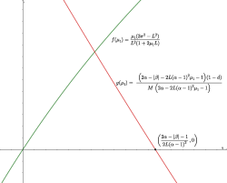
Figure 1. Maximum of $\lambda(\mu_{1})=\min\{f(\mu_{1}),g(\mu_{1})\}$.

4.2. Open problems

There are some points to be raised.

4.2.1. A time-varying delay feedback

If we consider $\alpha=0$, then the first main issue is how to prove the well-posedness of the problem. Note that, in this case, the semigroup theory cannot be applied. We believe that a variation of the approach introduced by Bona et al. in [5] can be adapted. However, this remains a promising research avenue, and the stabilization problem, in this case, needs to be investigated.

4.2.2. Variation of feedback-law

Considering two internal damping mechanisms and a linear combination of boundary damping and time-varying delay feedback, a similar result of Theorem 1.1 can be proved. Due to the restriction of the well-posedness problem, we can not remove the boundary damping. However, an open problem is to remove one internal damping mechanism and make $\beta=0$. We believe that the Calerman estimate shown in [1] can be used to investigate all these cases.

4.2.3. Optimal decay rate

Note that the second item of Subsection 4.1.2 gives the optimality of $\lambda$ for the stabilization problem related to the linear system associated with (1.7). In turn, it is still an open problem to obtain an optimal decay rate for both the linear and nonlinear problems without additional conditions for the parameters $\alpha$ and $\beta$.

References

• [1] J. A. Barcena-Petisco, S. Guerrero and A. F. Pazoto, Local null controllability of a model system for strong interaction between internal solitary waves, Communications in Contemporary Mathematics, 24, 1-30 (2022).
• [2] L. Baudouin, E. Crépeau and J. Valein, Two approaches for the stabilization of nonlinear KdV equation with boundary time-delay feedback, IEEE TAC 64:4, 1403–1414 (2019).
• [3] J. L. Bona, M. Chen, J.-C. Saut, Boussinesq equations and other systems for small-amplitude long waves in nonlinear dispersive media. I. Derivation and linear theory, J. Non. Sci. 12:4, 283–318 (2002).
• [4] J. L. Bona, M. Chen and J.-C. Saut, Boussinesq equations and other systems for small-amplitude long waves in nonlinear dispersive media. II. The nonlinear theory. Nonlinearity 17, 925–952 (2004).
• [5] J. L. Bona,S.-M. Sun and B.-Y. Zhang, A nonhomogeneous boundary-value problem for the Korteweg-de Vries Equation on a finite domain, Commun. PDEs, 8, 1391–1436 (2003).
• [6] J. V. Boussinesq, Théorie générale des mouvements qui sont propagés dans un canal rectangulaire horizontal, C. R. Acad. Sci. Paris 72, 755–759 (1871).
• [7] R. A. Capistrano–Filho, B. Chentouf, L. S. Sousa and V. H. Gonzalez Martinez, Two stability results for the Kawahara equation with a time-delayed boundary control, Z. Angew. Math. Phys. 74, 16 (2023).
• [8] R. A. Capistrano–Filho, E. Cerpa, and F. A. Gallego, Rapid exponential stabilization of a Boussinesq system of KdV–KdV Type, Communications in Contemporary Mathematics, 25:03, 2150111 (2023).
• [9] R. A. Capistrano–Filho and F. A. Gallego, Asymptotic behavior of Boussinesq system of KdV–KdV type, Journal of Differential Equations 265:6, 2341–2374 (2018).
• [10] R. A. Capistrano–Filho and A. Gomes, Global control aspects for long waves in nonlinear dispersive media, ESAIM:COCV, 29:7, 1-47 (2023).
• [11] R. A. Capistrano–Filho and V. H. Gonzalez Martinez, Stabilization results for delayed fifth-order KdV-type equation in a bounded domain, Mathematical Control and Related Fields, doi: 10.3934/mcrf.2023004.
• [12] R. A. Capistrano–Filho, V. H. Gonzalez Martinez and J.R. Muñoz, Stabilization of the Kawahara-Kadomtsev-Petviashvili equation with time-delayed feedback. [arXiv:2212.13552] (2022).
• [13] R. A. Capistrano–Filho, A. F. Pazoto and L. Rosier, Control of Boussinesq system of KdV-KdV type on a bounded interval, ESAIM: COCV, 25:58, 1–55 (2019).
• [14] B. Chentouf, Well-posedness and exponential stability results for a nonlinear Kuramoto-Sivashinsky equation with a boundary time-delay, Anal. Math. Phys., 11, 144 (2021).
• [15] B. Chentouf, Well-posedness and exponential stability of the Kawahara equation with time-delayed localized damping, Math. Methods Appl. Sci. 45, 10312–10330 (2022).
• [16] S. Micu, J. H. Ortega, L. Rosier and B.-Y. Zhang, Control and stabilization of a family of Boussinesq systems, Discrete Contin. Dyn. Syst., 24, 273–313 (2009).
• [17] S. Nicaise and C. Pignotti, Stability and instability results of the wave equation with a delay term in the boundary or internal feedbacks, SIAM J. Control Optim. 45:5, 1561–1585 (2006).
• [18] S. Nicaise, J. Valein, and E. Fridman, Stability of the heat and of the wave equations with boundary time-varying delays, Discrete Continuous Dynamical Systems-S.,2(3):559–581 (2009).
• [19] A. Pazy, Semigroups of Linear Operators and Applications to Partial Differential Equations, volume 44 of Applied Math. Sciences, Springer-Verlag, New York, 1983.
• [20] H. Parada, C. Timimoun, J. Valein. Stability results for the KdV equation with time-varying delay, Syst. Control Lett., 177, (2023), 105547.
• [21] A. F. Pazoto and L. Rosier, Stabilization of a Boussinesq system of KdV–KdV type, Syst. Control Lett. 57, 595–601 (2008).
• [22] T. Kato, Linear evolution equations of “hyperbolic” type. J. Fac. Sci. Univ. Tokyo Sect. I, 17, 241–258 (1970).
• [23] T. Kato, Quasi-linear equations of evolution, with applications to partial differential equations, In Spectral theory and differential equations, Springer, 25–70 (1975).
• [24] J. Valein, On the asymptotic stability of the Korteweg-de Vries equation with time-delayed internal feedback, Mathematical Control & Related Fields, 12:3, 667–694 (2022).