Radio Observations of Six Young Type Ia Supernovae

Abstract

Type Ia supernovae (SNe Ia) are important cosmological tools, probes of binary star evolution, and contributors to cosmic metal enrichment; yet, a definitive understanding of the binary star systems that produce them remains elusive. In this work we present early-time (first observation within 10 days post-explosion) radio observations of six nearby (within 40 Mpc) SNe Ia taken by the Jansky Very Large Array, which are used to constrain the presence of synchrotron emission from the interaction between ejecta and circumstellar material (CSM). The two motivations for these early-time observations are (1) to constrain the presence of low-density winds and (2) to provide an additional avenue of investigation for those SNe Ia observed to have early-time optical/UV excesses that may be due to CSM interaction. We detect no radio emission from any of our targets. Toward our first aim, these non-detections further increase the sample of SNe Ia that rule out winds from symbiotic binaries and strongly accreting white dwarfs. For the second aim, we present a radiation hydrodynamics simulation to explore radio emission from an SN Ia interacting with a compact shell of CSM, and find that relativistic electrons cannot survive to produce radio emission despite the rapid expansion of the shocked shell after shock breakout. The effects of model assumptions are discussed for both the wind and compact shell conclusions.

1 Introduction

Type Ia supernovae (SNe Ia) are the most homogeneous type of stellar explosion, and are therefore crucial cosmological tools (Branch, 1998; Riess et al., 2016; Abbott et al., 2019; Macaulay et al., 2019; Freedman et al., 2019). This homogeneity arises naturally as SNe Ia are the complete explosion of carbon-oxygen white dwarfs (CO WDs) of similar mass (Whelan & Iben, 1973; Bloom et al., 2012; Churazov et al., 2015). It is generally agreed that triggering an explosion requires the CO WD to interact with a binary companion star; however, the physical nature of this companion – and, thus, the evolution to explosion – is vigorously debated. Possible companions include red giant (RG), sub-giant (SG), [post-]asymptotic giant branch (AGB), main-sequence (MS), non-degenerate helium, He WD, or CO WD stars. The remaining mysteries of SN Ia progenitors are of general interest because SNe Ia impact a variety of topics in astrophysics, such as studies of cosmology, stellar evolution, next-generation gravitational wave signals, and galaxy evolution. Overviews of the SN Ia progenitor debate can be found in, e.g., Maoz et al. (2014) and Livio & Mazzali (2018).

Constraining SN Ia progenitors relies on indirect methods because, unlike some massive star supernovae, the expected progenitors are too dim to directly image in the vast majority of cases. One such method is the study of the circumstellar medium (CSM) surrounding the progenitor system. For example SG and RG companions are all expected to drive stellar winds that will produce an extended CSM (Seaquist & Taylor, 1990). MS/SG companions, as well as He WD companions, that are accreting onto the CO WD can produce CSM through non-conservative mass transfer (Huang & Yu, 1996). High accretion rates can also drive an optically thick wind (Hachisu et al., 1996). In any of these cases, we expect the wind to be hydrogen or helium rich, as the aforementioned accretion channels for SNe Ia involve these elements. In addition to these wind-like CSM profiles, more complex environments have been theoretically posited, such as a tidally ejected tail from the merger of two CO WDs (Raskin & Kasen, 2013), the ejected common envelope from the merger of two CO WDs or a CO WD and post-AGB star (Hamuy et al., 2003; Soker, 2013), or low-mass shells from a nova or recurrent novae (Moore & Bildsten, 2012). In these non-wind cases, the CSM may be confined rather than extended, may lack hydrogen or helium, and its distance from the progenitor system at time of explosion is unknown.

Constraining the circumstellar environment is primarily done by looking for signatures of the blast wave created by the collision of the SN Ia ejecta with the CSM. Shocks essentially redistribute the kinetic energy of the ejecta – donating some to ionizing the gas, heating the ions and electrons, amplifying magnetic fields, accelerating ions and electrons to relativistic speeds, and to radiation. The exact mechanism by which this is accomplished is still an active area of research, with particular interest in what share of the energy is given to each category and the downstream evolution of the components (e.g., Caprioli & Spitkovsky, 2014). Since shocks have the rare power to accelerate electrons to relativistic speeds and amplify magnetic fields, one of the hallmark signatures of SN-CSM interaction is radio emission from the synchrotron process. Although the interpretation of radio observations must then encounter the uncertainties in the shock physics related to both the magnetic fields and relativistic electrons, a key strength of this approach is that interaction with very low-density CSM is radio luminous although it would be invisible at most other wavelengths. X-ray emission is similarly produced in low-density interactions and has the additional benefit of not relying on the unknown physics of magnetic field amplification (Margutti et al., 2012, 2014). However, radio observations have the key benefit of being more sensitive and easier to mobilize – as they are ground-based – such that it is possible to attain a larger sample of constraining radio observations than it is with X-ray instruments. Furthermore, interpreting X-ray emission can be complicated without a spectrum to determine the relative contributions of thermal continuum, synchrotron continuum, inverse Compton upscattering of the supernova photosphere, and line emission (Chevalier & Fransson, 2006; Bochenek et al., 2018).

Given the benefits of radio observations to the SN Ia progenitor puzzle, there is a host of literature on the topic. Primarily, studies have focused on the existence of a wind-like CSM due to the theoretical strengths of the symbiotic (RG companion) progenitor channel in producing an explosion, which suggests that this channel should produce at least some SNe Ia (Iben & Tutukov, 1984; Branch et al., 1995). For example, a statistically significant set of radio observations near maximum light, assembled over decades, reveals that the symbiotic channel is likely a minor player in the overall SN Ia population (Chomiuk et al., 2016). The CSM in this case has a density profile $\rho_{\mathrm{csm}}=qr^{-2}$, with characteristic RG value $q\sim 5\times 10^{11}~{}\mathrm{g~{}cm^{-1}}$. In the cases of SN 2011fe and SN 2014J, deep radio limits probe even lower-density winds ($q\sim 10^{8}~{}\mathrm{g~{}cm^{-1}}$) and favor a double-degenerate merger scenario (Chomiuk et al., 2012; Pérez-Torres et al., 2014). Overall, the emerging picture for typical SN Ia progenitors at radio frequencies is that the symbiotic channel is disfavored, and the question now is how to whittle away at the remaining scenarios.

Most radio observations of SNe Ia have been obtained on timescales of weeks to a year after explosion (e.g. Chomiuk et al., 2016; Lundqvist et al., 2020), but here we argue two important reasons to search for CSM interaction at radio frequencies within a week of explosion.

The first reason is that interaction with low-density winds in other accretion scenarios, such as novae or weak winds during the stable burning phase of the white dwarf, will reach their peak radio luminosity at these times, so early radio observations allow these winds to be constrained.

The second reason is to reveal the nature of the early-time excess emission seen in some SNe Ia (e.g., Cao et al., 2015; Hosseinzadeh et al., 2017; Miller et al., 2018; Jiang et al., 2021; Deckers et al., 2022). There are many possible proposed origins for this emission, including interaction with CSM (Piro & Morozova, 2016; Jiang et al., 2021), the impact of the ejecta with the companion (Kasen, 2010), He-shell detonation (e.g. Polin et al., 2019), radioactive Ni⁵⁶ mixing in the ejecta (e.g. Piro & Morozova, 2016; Magee & Maguire, 2020; Sai et al., 2022), and the time evolution of the Dopper-shifted wavelength of prominent line absorption features (Ashall et al. (2022); but see also Hosseinzadeh et al. (2022)). Estimates of the CSM mass and extent needed to explain early-excess SNe Ia indicate dense, compact material. Hosseinzadeh et al. (2017) model the early excess of SN 2017cbv as the interaction of an SN Ia with a companion star but note that to obtain a similar signal with CSM interaction would require a CSM mass of $M_{\mathrm{csm}}\sim(0.01-0.1)~{}M_{\odot}$ extending to $R_{\mathrm{out}}\sim 4\times 10^{12}~{}\mathrm{cm}$, based on estimates given in Kasen (2010), to significantly decelerate the ejecta. We note that the binary separation for the best-fit model to the data of SN 2012cg (Marion et al., 2016) is similar to that found for SN 2017cbv, and would therefore require a similar CSM configuration. For the case of SN 2020hvf, the rapid evolution of the early excess emission is well fit by a CSM interaction model where the CSM has a mass $M_{\mathrm{csm}}=0.01~{}M_{\odot}$ extending to $R_{\mathrm{o}ut}=10^{13}~{}\mathrm{cm}$ (Jiang et al., 2021). For comparison, an RG wind would contain $\sim 3\times 10^{-9}~{}M_{\odot}$ of material within this radius. The CSM in the early-excess case is much more dense than a typical wind, yet radio emission is worth exploring because it is a “smoking gun” signature of interaction.

For these reasons, we have obtained deep observations of six SNe Ia within 10 days post-explosion as part of several VLA programs, which we present in this manuscript and analyze in the context of the low-density wind and compact shell CSM scenarios. In § 2 we present the radio upper limits derived from our observations. In § 3 we discuss our method for physically interpreting these limits; the vastly different density profiles between the low-density wind scenario (normal SNe Ia) and the compact shell scenario (early-excess SNe Ia) necessitates a separation in our modeling. We first looking at the low-density winds, for which we can use the Chevalier (1982a) self-similar hydrodynamic solution, and show that this method cannot be applied to the compact shell scenario, both because the shell is too dense and because it is truncated rather than extended (§ 3.1). We then describe how we use numerical radiation hydrodynamics to simulate the evolution of the shock in the compact CSM case in § 3.2. In § 3.3 we take a careful look at the relativistic electron populations in the shock region that are needed to create synchrotron emission, since we are concerned about whether these survive at all in the compact shell interaction, and discuss unknown physical parameters that affect radio analysis. § 3.4 describes the synchrotron light curve calculation for the self-similar solution. In § 4 we then present our analysis of the radio limits in the context of our models, showing how our sample significantly increases the number of SNe Ia that constrain low-density winds and taking a detailed look at the possibility of radio emission from early-excess SNe Ia. A summary of the work can be found in § 5.

2 Early-Time Observations of Type Ia Supernovae

Table 1: Summary of the young SNe Ia sample

Name	Locationa	Host galaxya	D (Mpc)b	Discovery Datea	Last Non-detectiona,e
SN 2019np	10:29:21.980 +29:30:38.30	NGC 3254	19.4	2019 Jan-09.66	2019 Jan-08.53
SN 2019einc	13:53:29.110 +40:16:31.33	NGC 5353	33	2019 May-01.47	2019 April-29.27
SN 2020rcq	11:57:14.680 +49:17:31.99	UGC 6930	11.1	2020 Aug-09.17	2020 Aug-07.17
SN 2020uxz	01:24:06.890 +12:55:17.26	NGC 514	35.5	2020 Oct-05.57	2020 Oct-05.40
SN 2021qvvd	12:28:02.920 +09:48:10.26	NGC 4442	14.7	2021 June-23.26	2021 June 21.37
SN 2021smj	12:26:46.560 +08:52:57.61	NGC 4411b	22.4	2021 July-08.27	2021 July-5.28

Note. — ^aObtained from Transient Name Server (TNS)

^bDistances measured from corresponding redshifts of the SN listed in TNS using the Cosmology Calculator (Wright, 2006),assuming $H_{0}=70$ $\mathrm{km/s/Mpc}$, $\Omega_{M}=0.3$ and $\Omega_{\Lambda}=0.7$.

^cMeasurements obtained from Pellegrino et al. (2020). Exhibits high-velocity features.

^d91bg-like, according to TNS

^eSince most SNe on TNS have photometry reported by multiple groups, we use the epoch of last non-detection reported by the discovery group on TNS, and if not available, the last non-detection by any of the other groups.

Table 2: Summary of radio observations of SNe Ia

Name	Project	Configa	Observation	Synthesized Beam	Ageb	F${}^{upper}_{6\mathrm{GHz}}$ (3$\sigma$)c	L${}^{upper}_{6\mathrm{GHz}}$ (3$\sigma$)d
	Code		Date	(arcsec$\times$arcsec)	(days)	($\mu$Jy)	($\times 10^{24}$ ergs/s/Hz)
SN 2019np	18B-162	C	2019 Jan-11.36	2.78 $\times$ 2.64	2.8	19.7	8.9
			2019 Jan-18.35	2.73 $\times$ 2.49	9.8	19.3	8.7
			2019 Jan-25.45	2.88 $\times$ 2.48	16.9	15.6	7.0
SN 2019ein	19A-010	B	2019 May-03.35	1.28$\times$1.27	3.9	17.9	23.4
			2019 May-11.04	2.20$\times$1.23	11.6	25.3	33.1
			2019 May-17.06	1.77$\times$1.99	17.6	23.5	31.0
SN 2020rcq	20B-355	B	2020 Aug-16.81	1.02 $\times$ 0.73	9.6	17.2	2.5
			2020 Aug-23.73	1.09$\times$0.74	16.6	17.0	2.5
			2020 Aug-25.8	0.94$\times$0.74	18.6	18.9	2.8
SN 2020uxz	20B-355	B	2020 Oct-06.28	0.87$\times$0.74	0.9	18.9	28.6
			2020 Oct-16.41	1.19$\times$0.87	11	18.1	27.4
			2020 Nov-05.28	0.90$\times$0.36	30.9	17.9	27.0
SN 2021qvv	21B-295	C	2021 June-24.99	3.18$\times$2.7	3.6	21.6	5.6
			2021 July-09.82	5.4$\times$2.89	18.5	28.0	7.3
			2021 July-16.99	3.07$\times$2.49	25.6	20.6	5.3
SN 2021smj	21B-295	C	2021 July-10.88	3.57$\times$3.08	5.6	18.1	10.9
			2021 July-15.99	3.17$\times$2.56	10.7	17.3	10.4

Note. — ^a VLA Configuration of observation.

^bSince last non-detection in Table 1.

^c3$\sigma$ upper limit to the 6 GHz flux density, described in Section 2.

^d3$\sigma$ upper limit to the 6 GHz spectral luminosity.

In this section, we describe our methodology for obtaining 6 GHz radio luminosity limits for our target SNe Ia. The targets and their limits are given in Tables 1 & 2.

We obtained VLA observations of young Type Ia SNe for the last few years within 40 Mpc (more distant SNe will not have deep enough constraints in radio). We used target-of-opportunity VLA programs to detect potential radio emission promptly after discovery as expected from main-sequence companions or close-in CSM shells. Once a SN was posted and spectroscopically classified as a Type Ia on the Transient Name Server (TNS), we triggered a VLA observation, along with typically 1–2 follow-up observations scheduled a week apart. Each observing block was 1 hr long in C-band (4–8 GHz), corresponding to an image RMS of roughly 4 $\mu$Jy/beam or a 3$\sigma$ luminosity limit of roughly $2.6\times 10^{25}$ ergs/s/Hz at 40 Mpc, enough to detect dense shells and winds predicted in SN Ia progenitor models (Chomiuk et al., 2012). Although the synchrotron emission from SNe will be brighter in L-band (1-2 GHz), we chose to observe in C-band due to its larger instantaneous bandwidth ($\sim$3.4 GHz, excluding RFI) and lower system temperature, giving increased sensitivity to faint sources for the same integration time. Moreover, C-band observations provide higher angular resolution images than L-band at any array configuration, which helps to distinguish emission from the SN location from other nearby confusing sources (e.g. bright galactic nuclei).

Our sample consists of six SNe newly observed with our VLA program between 2018-2021. With the exception of SN2019ein, whose radio observations have been published elsewhere (Pellegrino et al., 2020), we calibrated, imaged and recorded radio flux densities and upper limits of our targets in this paper.

Calibration was done with CASA pipeline versions 5.6–6.1. Aside from minor differences in implementation between versions, the pipeline applies online flags reported by the NRAO operator (e.g. antenna position changes) and performs iterative flagging and calibration of the raw visibility data. Calibration consists of delay, bandpass and absolute flux density scale calibration with one of VLA’s primary calibrator, and antenna-based complex gain calibration using a secondary calibrator close to the target location and observed in between target observations. Flagging is done with the automated rflag algorithm in between calibration steps to remove corrupted measurements. Each pipeline calibrated dataset is manually inspected and further flagged if RFI remains, and then passed on to imaging.

Imaging was performed using the tclean task. The imaging region extended to a primary beam level of 5$\%$ to ensure all outlying sources were deconvolved in order to obtain maximum sensitivity at the image center where the SN target is located. The cell size was chosen to sample the full width at half maximum of the effective point-spread-function (PSF) with 4 pixels. For all images, we used gridder=standard, which resamples the visibility data onto a regular grid using a prolate spheroidal function. Gridding options that include widefield, direction-dependent corrections exist in CASA, but are computationally expensive, and likely unnecessary since our object of interest is at the phase center. For deconvolution, we use multi-term multi-frequency synthesis with nterms=2 to account for the frequency-dependent structure of the sky. Briggs weighting with robust=0 was applied to the data in order to balance point source sensitivity with sidelobe contamination from bright sources. With these settings, we cleaned our images for a maximum of 10⁴ iterations, or once the image RMS is less than three times the peak residual in the image (nsigma=3). In cases where the RMS of the final image is limited by dynamic range due to bright sources, we carried out phase-only self-calibration to further improve the image.

No SN was detected in any of our radio images. We provide the results of our observations in Table 2. The 6 GHz 3$\sigma$ upper limit on the flux density for each SN is defined as the 6 GHz flux density at the pixel location of the SN, plus the 3$\sigma$ RMS noise calculated in a circular region around the SN. In the case where the flux density at the pixel location is negative, we only use the 3$\sigma$ RMS noise. The radii of the regions ranged from 6-14^′′, as they were adjusted to be large enough to contain sufficient pixels for a robust RMS calculation, but small enough to represent the local RMS and exclude any visible adjacent sources or artifacts. The 6 GHz 3$\sigma$ luminosity is then given by $\left(1.2\times 10^{21}\mathrm{ergs\ s^{-1}\ Hz^{-1}}\right)S_{\mu jy}D_{Mpc}^{2}$ as per Eq. 3 in Chomiuk & Wilcots (2009), where $S_{\mu jy}$ is the 3$\sigma$ flux upper limit in $\mu$Jy, and $D_{Mpc}$ is the distance to the SN in Mpc, given in Table 1.

One object in our sample, SN 2019np, is observed to have a modest early excess in the bolometric light curve, but this excess is well explained by ⁵⁶Ni mixing in the ejecta (Sai et al., 2022).

3 Ejecta-CSM Interaction Models

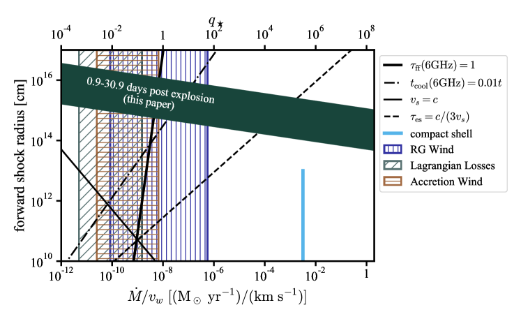
In this section, we describe the hydrodynamic and radio synchrotron light curve models used in this paper to analyze the early-time radio observations. § 3.1 describes the analytic hydrodynamic solution we employ for constraining the presence of low-density winds, and § 3.2 describes our radiation hydrodynamics simulation for approaching the compact shell scenario. We review the model for the calculation of the electron acceleration and synchrotron light curves that result from the interaction in § 3.3 & 3.4. Figure 1 provides a visual synopsis of this section, showing the shock radii probed by our observations, the CSM configurations of interest, and the various limiting factors for our analysis. In § 4, we will use the methodology presented here to physically interpret our radio limits.

Figure 1: Quantities of interest for our analysis, assuming the forward shock radius evolves according to the self-similar solution for interaction with a wind. The shock radii probed by our observations are shown by the dark green band, hatched regions show wind CSM configurations we investigate, and the thick blue line describes our compact shell simulation. The assumptions of the hydrodynamic model are valid for $R_{f}$ above the $v_{s}=c$ (thin solid) and $\tau_{\mathrm{es}}=c/(3v_{s})$ (dashed) lines. The $\tau_{\mathrm{ff}}$ (thick solid) line shows where an infinite wind becomes optically thin to external free-free absorption – right of this line, 6 GHz emission is absorbed. The $t_{\mathrm{cool}}=0.01t$ (dot-dashed) line shows the relativistic electron cooling boundary – right of this line, the emitting volume is reduced.

3.1 Wind Interaction Hydrodynamics

For the interaction with steady winds, we employ the self-similar model of Chevalier (1982a). For interaction with a wind-like CSM, this model has performed well in fitting the radio data of core-collapse SNe (e.g., Weiler et al., 1986; Soderberg et al., 2005).

3.1.1 Ejecta Density Profile for Steady Wind Interaction

For wind interaction, we will approximate the SN Ia ejecta as a broken power-law (Chevalier & Fransson, 1994), which provides a reasonable approximation to the structure found in hydrodynamical models of SNe. As in Kasen (2010), we use $\rho\propto r^{-1}$ to describe the inner ejecta mass-density profile. We note that the detailed structure of the inner ejecta is only relevant in this work in setting the fraction of the total mass that is in the outer ejecta. We assume the ejecta are in homologous expansion such that $v=r/t$, with $v$ being the ejecta speed and $t$ time. The transition point between the inner and outer ejecta occurs at speed

$$v_{t}=(1.014\times 10^{4}~{}\mathrm{km~{}s^{-1}})~{}(E_{51}/M_{\mathrm{c}})^{1/2},$$ (1)

where $M_{\mathrm{c}}=M_{\mathrm{ej}}/(1.44~{}M_{\odot})$ is ejecta mass in units of the Chandrasekhar mass and $E_{51}=E/(10^{51}~{}\mathrm{erg})$ is the explosion energy. We use $M_{c}=1$ and $E_{51}=1$. The outer ejecta density profile is given by

$$\rho_{\mathrm{ej}}(r)=\frac{0.124M_{\mathrm{ej}}}{(v_{t}t)^{3}}\left(\frac{r}{v_{t}t}\right)^{-10},$$ (2)

which can be written as

$$\rho_{\mathrm{ej}} = \rho_{\mathrm{0,ej}}t^{7}r^{-10},$$ (3)

$$\rho_{\mathrm{0,ej}} \equiv (3.6\times 10^{9}~{}\mathrm{g~{}cm^{-3}})^{10}M_{c}^{-5/2}E_{51}^{7/2}~{}.$$ (4)

The above equations describe the density and velocity profile for the SN Ia ejecta we assume when using the self-similar model for the wind interaction case.

3.1.2 Density Profile of Steady Winds

A steady wind can be described by the density profile $\rho=qr^{-2}$. For consistency with Chevalier & Fransson (2006) and Chomiuk et al. (2016), we will adopt the normalization $q_{*}=q/(5\times 10^{11}~{}\mathrm{g~{}cm^{-1}})$, such that $q_{*}=1$ corresponds to $\dot{M}/v_{w}=10^{-8}~{}\mathrm{(M_{\odot}~{}yr^{-1})/(km~{}s^{-1})}$ – though we note that this variable is called “$A_{*}$” in those works. Thus,

$$\rho_{\mathrm{csm}}=(5\times 10^{-19}~{}\mathrm{g~{}cm^{-3}})q_{\star}\left(\frac{r}{10^{15}~{}\mathrm{cm}}\right)^{-2}$$ (5)

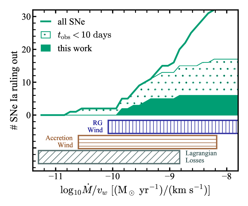
Although the self-similar model constrains $q$ without reference to the wind origin, throughout this work we will reference several physically motivated winds. First, there is the canonical symbiotic system in the single-degenerate scenario, with a CO WD accreting a RG wind. For this, we assume wind velocities span $v_{w}\sim(9-60)~{}\mathrm{km~{}s^{-1}}$ and mass-loss rates span $\dot{M}\sim(5\times 10^{-9}-5\times 10^{-6})~{}\mathrm{M_{\odot}~{}yr^{-1}}$ (Seaquist & Taylor, 1990). Second, we consider the properties of an optically thick wind from high accretion rates (Hachisu et al., 1996), for which we use a velocity span of $v_{w}\sim(300-4,000)~{}\mathrm{km~{}s^{-1}}$ and consider mass-loss rates $\dot{M}\sim(10^{-7}-2\times 10^{-6})~{}\mathrm{M_{\odot}~{}yr^{-1}}$. These winds could be in play in either hydrogen or helium accretion scenarios (Hachisu et al., 1999), but this mass-loss scenario may not be in effect at the time of explosion as it requires a high accretion rate. Finally, we show the hypothetical case of non-conservative mass transfer via losses from the outer Lagrangian point in a Roche Lobe overflow scenario (Huang & Yu, 1996). Here, we assume the accretion rate is appropriate for stable burning (e.g., Shen & Bildsten, 2007) and the mass-loss rate is a modest 1% of the accretion rate, such that $v_{w}\sim(20-600)~{}\mathrm{km~{}s^{-1}}$ and $\dot{M}\sim(10^{-9}-3\times 10^{-8})~{}\mathrm{M_{\odot}~{}yr^{-1}}$. These winds are shown in Figure 1 as the “RG wind,” “Accretion Wind,” and “Lagrangian losses” regions, respectively.

3.1.3 Steady Wind Shock Hydrodynamics

We will leverage the asymptotic self-similar solution of Chevalier (1982a) for the hydrodynamics of the shock evolution. Per this model, the contact discontinuity radius (the boundary between the ejecta and CSM) evolves as

$$R_{c}=\left(\frac{A\rho_{\mathrm{0,ej}}}{q}\right)^{1/(n-s)}t^{(n-3)/(n-s)}~{},$$ (6)

where $\rho_{\mathrm{ej}}=g^{n}t^{n-3}r^{-n}$, $\rho_{\mathrm{csm}}=qr^{-s}$, $t$ is time, and $A$ is a numerical constant that depends on $s$ and $n$. From our ejecta and CSM density profiles, we identify $g^{n}=\rho_{\mathrm{0,ej}}$, $n=10$, and $s=2$, such that $A=0.067$, $R_{f}/R_{c}=1.239$, $R_{r}/R_{c}=0.984$, and thus,

$$R_{f,15}=4.22~{}M_{c}^{-5/16}E_{51}^{7/16}q_{\star}^{-1/8}t_{10}^{7/8}~{},$$ (7)

where $R_{f,15}=R_{f}/(10^{15}~{}\mathrm{cm})$.

Since our work involves very early-time observations and we consider interaction with dense CSM, we will here revisit two underlying assumptions of the model that can affect the shock hydrodynamics.

Assumption 1: Non-relativistic Shock

As can be seen in Equation 7, the shock is decelerating over time, and the speed of the shock becomes infinite at $t=0$. We must ensure that our early-time observations are not taken at a time when this model would imply a relativistic shock, since the model is non-relativistic. With the equation for $R_{c}$, time can be written

$$t_{10} = 0.193~{}M_{c}^{5/14}E_{51}^{-1/2}R_{f,15}^{8/7}q_{*}^{1/7},$$ (8)

where $t_{10}=t/(10~{}\mathrm{days})$. The forward shock speed is $v_{s}=[(n-3)/(n-s)]R_{f}t^{-1}$, so

$$v_{s,9} = 5.25(M_{c}^{5/2}E_{51}^{-7/2}q_{*}R_{f,15})^{-1/7}$$ (9)

$$= 4.28(M_{c}^{5/2}E_{51}^{-7/2}q_{\star}t_{10})^{-1/8}~{},$$ (10)

where $v_{s,9}=v_{s}/(10^{9}~{}\mathrm{cm~{}s^{-1}})$. Then, the constraint that $v_{s}$ is less than the speed of light, $c$, can be written as the constraint that the forward shock radius is

$$R_{f,15}\geq(5.06\times 10^{-6})~{}M_{c}^{-5/2}E_{51}^{7/2}q_{\star}^{-1}~{},$$ (11)

where $R_{f,15}=R_{f}/(10^{15}~{}\mathrm{cm})$. This constraint is shown in Figure 1 and is not a concern for our analysis.

As we are discussing shock speed, we note that the ram pressure of the shock is

$$\frac{\rho_{\mathrm{csm}}v_{s}^{2}}{\mathrm{erg~{}cm^{-3}}} = 13.79M_{c}^{-5/7}E_{51}q_{*}^{5/7}R_{f,15}^{-16/7}$$ (12)

$$= 0.51q_{*}t_{10}^{-2}~{},$$ (13)

which will be used to determine post-shock energy densities.

Assumption 2: Equation of State

The model we are using assumes a gamma-law equation of state with $\gamma_{\mathrm{ad}}=5/3$, but the high densities of some of the CSM configurations of interest may be radiaton pressure dominated ($\gamma_{\mathrm{ad}}=4/3$), which would violate this assumption. We can estimate the boundary as in Chevalier & Fransson (1994), arguing that photons are not trapped by the gas so long as the electron scattering optical depth obeys

$$\tau_{\mathrm{es}}<c/(3v_{s})~{}.$$ (14)

Using

$$\tau_{\mathrm{es}}=\kappa_{\mathrm{es}}(4\rho_{\mathrm{csm}})(1-R_{r}/R_{f})R_{f},$$ (15)

where the electron scattering opacity is $\kappa_{\mathrm{es}}=0.4~{}\mathrm{cm^{2}~{}g^{-1}}$, we arrive at the condition that photons can escape the shock region when

$$R_{f} > \left(\frac{\dot{M}}{v_{w}}\right)^{\frac{n-4}{n-2}}(4\pi A\rho_{\mathrm{0,ej}})^{\frac{1}{n-2}}$$ (16)

$$\times \left(\frac{R_{f}}{R_{c}}\right)\left(1-\frac{R_{r}}{R_{f}}\right)^{\frac{n-3}{n-2}}\left(\frac{(n-3)(3\kappa_{\mathrm{es}})}{(n-2)(\pi c)}\right)^{\frac{n-3}{n-2}}.$$ (17)

For the ejecta and CSM used in this work, this condition is

$$R_{f}>(2.81\times 10^{11}~{}\mathrm{cm})~{}q_{\star}^{3/4}~{}.$$ (18)

This constraint is shown in Figure 1, where we see that radiation hydrodynamics calculations are required for the highest densities. As mentioned in § 1, compact shells must have $q_{\star}\gtrsim 10^{5}$ to explain early-excess SNe Ia and are clearly radiation pressure dominated, necessitating numerical radiation hydrodynamic simulations to capture their shock evolution.

3.2 Compact Shell Interaction Radiation Hydrodynamics

As shown in the last section, the CSM shells expected to produce optical excess from interaction are in a regime where shocks are radiation dominated. Therefore, to model the interaction of SNe Ia with compact shells of CSM, we use the SuperNova Explosion Code (SNEC), a one-dimensional Lagrangian radiation hydrodynamics code (Morozova et al., 2015) to extend the set of compact CSM interaction models presented in Piro & Morozova (2016). We refer the reader to these works for further detail, but we summarize key points of the modeling below.

There are several reasons to expect that we would not detect radio emission during the interaction itself. First, because the CSM is truncated at a very small radius ($\sim 10^{13}~{}\mathrm{cm}$) so a radio observation would have to be obtained within about an hour post-explosion to observe at this phase. Second, the CSM is so dense that radio emission will be easily absorbed by the pre-shock CSM (see § 3.4 for a calculation). However, in the case of adiabatic shocks with truncated CSM, Harris et al. (2016) showed that there is a long tail to the radio light curve after the shock has crossed the CSM. Numerical simulations are required to capture the evolution of the shocked CSM as it rarefies to assess whether such a tail could be observed in the compact shell interaction case.

3.2.1 Ejecta Density Profile for Compact Shell Interaction

The WD explodes as part of the SNEC simulation, so the ejecta density profile in this case is generated within the simulation. The WD density profile is that of a $1.25~{}M_{\odot}$ WD evolved with the Modules for Experiments in Stellar Astrophysics (MESA) code (Paxton et al., 2011). Its composition is 49% ¹²C, 49% ¹⁶O, and 2% ²⁰Ne by mass. Since SNEC lacks a nuclear reaction network, the composition does not change post-explosion, except that ⁵⁶Ni is added to the domain. As in Piro & Morozova (2016), we input $0.5~{}M_{\odot}$ of ⁵⁶Ni (the mass fractions of other elements are adjusted to account for this). For the extent of the ⁵⁶Ni distribution, we use a boxcar width of $0.125~{}M_{\odot}$, which matches the $V$-band rise of SN 2011fe best of the Ni-56 distributions explored in Piro & Morozova (2016). More distributed nickel causes a shallower light curve rise, as seen in SN 2019np (Sai et al., 2022).

3.2.2 Compact Shell Density Profiles

Motivated by several WD merger models (Pakmor et al., 2012; Schwab et al., 2012; Shen et al., 2012), the compact shell interaction models produced by Piro & Morozova (2016) have $M_{\mathrm{csm}}=0.1$ and $R_{\mathrm{out}}=(10^{9}-10^{12})~{}\mathrm{cm}$, and a density profile

$$\rho_{\mathrm{shell}}=q_{\mathrm{shell}}r^{-3}~{},$$ (19)

where $q_{\mathrm{shell}}$ can be found via $M_{\mathrm{csm}}=4\pi q_{\mathrm{shell}}\ln(R_{\mathrm{out}}/R_{\mathrm{WD}})$, with $R_{\mathrm{WD}}$ the white dwarf outer radius. As it is supposed to have originated from the merger of two WDs, we use the same composition for the CSM as for the WD zones (49% ¹²C, 49% ¹⁶O, 2% ²⁰Ne). In this work, we present a model with $M_{\mathrm{csm}}=0.01~{}M_{\odot}$ and $R_{\mathrm{out}}=10^{13}~{}\mathrm{cm}$, which describes the CSM of the early-excess SN 2020hvf (Jiang et al., 2021). Our simulation differs from that of Jiang et al. (2021), however, because we assume normal SN Ia ejecta properties and model the first day post-explosion with increased time sampling (since our focus is the evolution of the shock). This model is illustrated in Figure 1, using $\dot{M}/v_{w}=M_{\mathrm{csm}}/R_{\mathrm{out}}$.

3.2.3 Radiation Hydrodynamics with SNEC

In the compact shell CSM case, the high densities imply that the shock is radiation pressure dominated (Equation 18). At the same time, these compact shells are of finite extent, so there will be a shock breakout (the shocked gas becomes optically thin) near the time that the shock front reaches the edge of the CSM, after which point the system becomes gas pressure supported. Due to this complex behavior and the necessity of following the evolution of the shocked gas after breakout, we employ the SNEC radiation hydrodynamics code to explore this scenario. As in Piro & Morozova (2016), our simulations use piston-driven explosions to unbind the WD. The domain is 400 zones covering the entire WD and CSM, with increased mass resolution at the inner and outermost zones. The output includes the evolution of hydrodynamic variables in each zone, which we can then use in calculations of interest. Furthermore, SNEC output provides the evolution of the shock speed and radius which we utilize to identify the immediate postshock zones.

3.3 Electron Distribution

In any interaction scenario, radio emission through the synchrotron process depends on relativistic electrons. Synchrotron emission arises from electrons accelerated to relativistic speeds through repeated interactions with the amplified and turbulent magnetic field in the shocked gas (see, e.g., Marcowith et al., 2020, for a review). Then, for Lorentz factors between $\gamma_{\min}$ and $\gamma_{\max}$, the electron density is described by a power-law distribution

$$N_{e,\mathrm{nt}}(\gamma)d\gamma=C_{\gamma}\gamma^{-p}d\gamma,$$ (20)

where $n_{e,\mathrm{nt}}=\int N_{e,\mathrm{nt}}d\gamma$ is the number density of electrons in the power-law distribution. Therefore, to describe the relativistic electrons that will create synchrotron emission, we must determine $C_{\gamma}$, $\gamma_{\min}$, $\gamma_{\max}$, and $p$. In this work, we follow the method of Chevalier & Fransson (2006) for accomplishing this, as we detail below.

The value of $p$ is expected to be $2<p<3$. Chevalier (1998) takes $p=3$ as a reference value based on observations of SNe Ibc. In other contexts, the index may differ slightly; for example, observations of supernova remnants (SNRs) have found $p=2.2-2.5$ (Green, 2019). Diesing & Caprioli (2021) suggest that the steeper power-law index in radio SNe may be explained by their faster shocks and higher magnetic field energy densities. In this work, we will use $p=3$ as our fiducial value because we expect the shock speeds to be more similar to SNe Ibc than to SNRs.

We assume $\gamma_{\max}=\infty$ in our calculations. Since the energy density distribution is a steep power-law, this assumption does not significantly affect our analysis.

To determine $C_{\gamma}$ and $\gamma_{\min}$, we adopt the common formalism of assuming that the energy density in the power-law electron distribution, $u_{e}$, is a time-independent fraction of the shock energy density

$$u_{e}=\epsilon_{e}\rho_{\mathrm{csm}}v_{s}^{2},$$ (21)

where $\rho_{\mathrm{csm}}$ is the pre-shock CSM mass density. Clearly, $\epsilon_{e}<1$, but its value is not entirely certain. Studies of gamma-ray afterglows, for example, find $\epsilon_{e}\sim 0.1$ (Panaitescu & Kumar, 2002; Yost et al., 2003; Chevalier et al., 2004; Marongiu et al., 2022). Simulations of particle acceleration in shocks also find that about $10\%$ of the postshock energy is in relativistic ions (Caprioli & Spitkovsky, 2014), so, if electrons and ions equilibrate, then $\epsilon_{e}\sim 0.1$; however, in low-density winds it is unlikely that they do equilibrate, which would suggest $\epsilon_{e}\ll 0.1$. A recent study of supernova remnants finds a wide range of $\epsilon_{e}\sim 10^{-4}-0.08$ (Reynolds et al., 2021). We take $\epsilon_{e}=0.1$ as our fiducial value.

Using the $\epsilon_{e}$ formalism we then have

$$n_{e,\mathrm{nt}}=\int_{\gamma_{\min}}^{\infty}C_{\gamma}\gamma^{-p}d\gamma,$$ (22)

$$\epsilon_{e}\rho_{\mathrm{csm}}v_{s}^{2}=m_{e}c^{2}\int_{\gamma_{\min}}^{\infty}C_{\gamma}\gamma^{-p+1}d\gamma$$ (23)

thus,

$$C_{\gamma}=(p-1)n_{e,\mathrm{nt}}\gamma_{\min}^{p-1}$$ (24)

$$\gamma_{\min}=\frac{p-2}{p-1}\frac{\epsilon_{e}\rho_{\mathrm{csm}}v_{s}^{2}}{m_{e}c^{2}n_{e,\mathrm{nt}}}~{}.$$ (25)

If a fraction $f_{\mathrm{nt}}$ of the total electrons in the shocked region are in the power-law component, then $n_{e,\mathrm{nt}}=\eta f_{\mathrm{nt}}\rho_{\mathrm{csm}}/(\mu_{e}m_{p})$, where $\mu_{e}=\rho/(n_{e}m_{p})$ and $\eta$ is the mass compression ratio. Thus,

$$\gamma_{\min} = 2.04\frac{p-2}{p-1}\left(\frac{\mu_{e}\epsilon_{e}}{\eta f_{\mathrm{nt}}}\right)v_{s,9}^{2}~{},$$ (26)

which can be evaluated as a function of shock radius or time since explosion via Equations 9 & 10. We assume $f_{\mathrm{nt}}=1$ to begin with, but in the case that this results in $\gamma_{\min}<1$, we decrease $f_{\mathrm{nt}}$ such that $\gamma_{\min}=1$. Thus, as noted in Chevalier & Fransson (2006), we are accounting for the fact that a result of $\gamma_{\min}<1$ indicates a substantial population of thermal electrons.

In the limit that $\gamma_{\min}=1$,

$$C_{\gamma}=(2.99\times 10^{5}~{}\mathrm{cm^{-3}})(p-1)\frac{\eta f_{\mathrm{nt}}}{\mu_{e}}q_{\star}R_{f,15}^{-2}~{},$$ (27)

but for $\gamma_{\min}>1$ and $p=3$,

$$C_{\gamma}=(4.75\times 10^{8}\mathrm{cm^{-3}})\frac{\mu_{e}\epsilon_{e}^{2}}{\eta f_{\mathrm{nt}}}M_{c}^{-10/7}E_{51}^{2}q_{*}^{3/7}R_{f,15}^{-18/7}~{}.$$ (28)

3.3.1 Cooling of Relativistic Electrons

Synchrotron emission will be diminished if relativistic electrons in the shocked ejecta cool. A relativistic electron of energy $\sim\gamma m_{e}c^{2}$ will cool by the synchrotron process in a time

$$t_{\mathrm{cool}}\sim\frac{\gamma m_{e}c^{2}}{\frac{4}{3}\sigma_{T}cu_{B}\gamma^{2}}$$ (29)

where $u_{B}=\epsilon_{B}\rho_{\mathrm{csm}}v_{s}^{2}$ can be calculated from Equation 13.

The formalism of assuming the magnetic field energy density $u_{B}=B^{2}/8\pi$ is a constant fraction $\epsilon_{B}$ of the internal energy density is in common use for astrophysical shocks; yet, there is significant debate surrounding the value of $\epsilon_{B}$. Analyses of GRB afterglows find a wide range of values, $\epsilon_{B}=7.4\times 10^{-4}-0.2$ (e.g., Chevalier et al., 2004; Panaitescu & Kumar, 2002; Yost et al., 2003). Studies of core-collapse supernovae interacting with the progenitor wind also find a wide range – for example, $\epsilon_{B}\sim 10^{-3}q_{\star}^{-1}$ derived for the Type Ic SN 2002ap (Björnsson & Fransson, 2004), $\epsilon_{B}\sim 3\times 10^{-4}$ for the Type IIb SN 2011dh (Horesh et al., 2013), or $\epsilon_{B}=0.24(0.003)$ for the Type II SN 1987A (SN 1979C) (Chevalier, 1998). Taking a theoretical approach, Duffell & Kasen (2017) posit that magnetic fields should be amplified by the turbulent cascade of the Rayleigh-Taylor instability that occurs naturally in astrophysical shocks, and derive a lower bound of $\epsilon_{B}=3\times 10^{-3}$ from this mechanism. In this work, we take $\epsilon_{B}=0.1$ to be our fiducial (or “default”) value, because this is typical value assumed in SN Ia literature; but when we perform our analysis we consider a range $\epsilon_{B}=3\times 10^{-3}-0.3$, i.e., ranging from the turbulence limit to essentially the maximum possible value from equipartition.

After assuming a value of $\epsilon_{B}$, we then have

$$\frac{t_{\mathrm{cool}}}{t}\sim 695\gamma^{-1}\left(\frac{\epsilon_{B}}{0.1}\right)^{-1}q_{\star}^{-1}t_{10}~{}.$$ (30)

Alternatively, we can use the cyclotron frequency, which for the wind interaction models is

$$\nu_{\mathrm{cyc}}=\sqrt{\frac{2}{\pi}}\frac{q_{e}}{m_{e}c}\sqrt{u_{B}}=(3.18~{}\mathrm{MHz})t_{10}^{-1}\left(\frac{\epsilon_{B}}{0.1}q_{\star}\right)^{1/2}~{},$$ (31)

to substitute

$$\gamma=\sqrt{\nu/\nu_{\mathrm{cyc}}}=43.45\sqrt{\nu_{6}t_{10}}\left(q_{\star}\frac{\epsilon_{B}}{0.1}\right)^{1/4},$$ (32)

where $\nu_{6}=\nu/(6~{}\mathrm{GHz})$, and have

$$\frac{t_{\mathrm{cool}}}{t}\sim 16\left(\frac{t_{10}}{\nu_{6}}\right)^{1/2}\left(q_{\star}\frac{\epsilon_{B}}{0.1}\right)^{-3/4}$$ (33)

In Figure 1 we show the limit of what may be called rapid cooling, where $t_{\mathrm{cool}}/t=1\%$.

This equation is useful for anticipating that the compact shell CSM will suffer from very rapid cooling of the relativistic electron population, and relativistic electrons would only be present immediately behind the shock front. Already, we expected that detecting radio emission during interaction would be impossible because interaction ends within hours post-explosion and pre-shock CSM would absorb the radio emission – the only hope was catching a radio “tail” from the expanding post-shock shell. Given the rapid cooling time for relativistic electrons, we now see that a radio detection also hinges on the post-interaction expansion being rapid enough to slow down relativistic electron cooling. This is our motivation for performing a SNEC simulation with the same setup as Piro & Morozova (2016), but with finer time resolution of the output hydrodynamic grid focused on the earliest phases of the SN evolution that allows an exploration of how the gas evolves during and immediately after interaction with the compact CSM shell.

We can calculate the cooling time just behind the shock front in the SNEC simulation via Equation 29. We focus on the immediate post-shock region because electrons that cool immediately are not expected to be re-accelerated downstream, so the immediate post-shock region contains the electrons of interest. The hydrodynamic quantities just behind the shock are obtained as follows. While $R_{f}\leq R_{\mathrm{out}}$, SNEC tracks the shock properties (zone index, radius, speed) over time with finer time resolution than the output snapshots of the entire domain, and provides the shock solution as output. We use a cubic interpolation (via scipy.interpolate.interp1d) of the shock zone index over time to calculate the zone index of the shock at the snapshot times (rounding down), and use the cell-centered values of hydrodynamic variables from the preceding cell to represent conditions just behind the shock. We calculate the hydrodynamic time using the radius and speed at the center of the cell just behind the shock; though we note that $t_{\mathrm{hydro}}\sim t$. For the cooling time calculation, we have the specific internal energy and the mass density ($\rho$) in the cell, whose product is the internal energy density, $u_{\mathrm{int}}$. While the shock is in the CSM, $u_{\mathrm{int}}=u_{e}/\epsilon_{e}=u_{B}/\epsilon_{B}$. Since the cooling time depends on $\epsilon_{B}$, we explore both $\epsilon_{B}=0.003$ and $0.1$. If relativistic electrons do not cool rapidly in the immediate post-shock region, then these $\epsilon_{B}$ values also represent the possible change in $\epsilon_{B}$ downstream from the shock (Crumley et al., 2019). For times after $R_{f}=R_{\mathrm{out}}$, we use the properties of the second-to-last zone of the domain to calculate the cooling time of the outermost CSM as it rarefies. After the shock has swept over the CSM, we assume the number of (isotropic) magnetic field lines is conserved in the expanding gas such that $B\propto r^{-2}$, i.e., $u_{B}\propto r^{-4}$.

3.4 Synchrotron Light Curve

Our method for generating synchrotron radio light curves is as in Chomiuk et al. (2016), which is a restatement of the equations from Chevalier (1998). Since we consider higher wind densities than in Chomiuk et al. (2016), we furthermore include the free-free absorption equations from Chevalier (1982b). We note that a similar procedure could be used to approximate a light curve from the SNEC compact shell simulation, but is not performed in this work as we find that relativistic electrons do not survive ($C_{\gamma}=0$), as we will show in §4.2.

The flux density assuming synchrotron self-absorption (SSA) only and $p=3$ is

$$F_{\nu}=6.67\times 10^{-30}R_{f}^{2}D_{L}^{-2}B^{-1/2}\nu^{5/2}\left[1-e^{-\left(\nu/\nu_{1}\right)^{7/2}}\right]~{},$$ (34)

where $D_{L}$ is the distance to the target, $\nu$ is frequency, $B$ is the magnetic field strength, and all quantities are in cgs units such that the final units of $F_{\nu}$ are $\mathrm{erg~{}s^{-1}~{}cm^{-2}~{}Hz^{-2}}$. The quantity $\nu_{1}$ is the frequency at which the SSA optical depth is unity, and is given by

$$\nu_{1}=(47.6~{}\mathrm{MHz})R_{f}^{2/7}f^{2/7}C_{\gamma}^{2/7}B^{5/7}~{},$$ (35)

where $f$ is the filling factor of the emitting region, defined via $V_{\mathrm{em}}=f(4\pi R_{f}^{3}/3)$. Then, for $n=10$ and $s=2$, we use $f=1-(R_{r}/R_{f})^{3}=0.5$ (Chevalier, 1982a).

Since the CSM densities considered in this work span a wide range and the observations cover very early times, we will consider the effects of free-free absorption by the unshocked CSM in addition to the synchrotron self-absorption from the shocked CSM. We use Equation 22 of Chevalier (1982b), to compute the free-free optical depth in the case of an infinite-extent wind as

$$\tau_{\mathrm{ff}}=4.35~{}q_{\star}^{2}R_{f,15}^{-3}\left(\frac{\nu}{6~{}\mathrm{GHz}}\right)^{-2}$$ (36)

where we have replaced the maximum material velocity with $R_{r}/t$. We account for external absorption by multiplying the flux from Equation 34 by $\exp(-\tau_{\mathrm{ff}})$. Due to the early times of our observations, free-free absorption is dominant even for low mass-loss rates.

4 Results

In this section, we use the calculations described in § 3 to analyze our early-time radio dataset and draw conclusions about the progenitor systems for these SNe Ia.

4.1 Wind-Like CSM

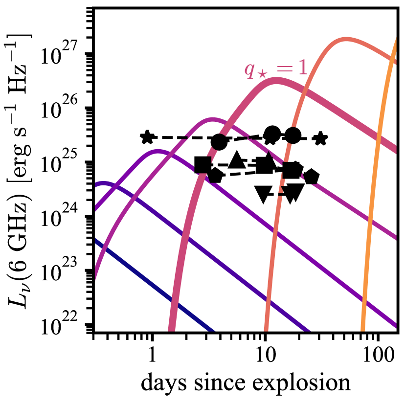
Figure 2 shows the synchrotron light curves that result from interaction with a wind with density $10^{-4}\leq q_{\star}\leq 10^{2}$ compared to the limits obtained for our six targets. We see that winds with $q_{\star}<10^{-2}$ peak within a day post-explosion and therefore escape detection even from the earliest observations. At higher densities than this, $10^{-2}<q_{\star}<1$, we see a power-law rise characteristic of the dominance of synchrotron self-absorption. In the $q_{\star}=0.1,1$ cases, we see that this power-law rise is preceded by an exponential rise, and the two highest density cases have exponential rises; this is the signature of diminishing free-free absorption. From this figure it is easy to see that our early-time observations will have the most constraining power for $10^{-2}<q_{\star}<10$ winds, which includes most of the CSM wind scenarios we are investigating as shown in Figure 1.

Figure 2: Wind interaction 6 GHz synchrotron light curves, assuming fiducial parameters, in decade increments of $q_{\star}$ from $10^{-4}$ (blue) to $10^{2}$ (yellow-orange) – i.e., $\dot{M}/v_{w}=10^{-12}-10^{-6}~{}\mathrm{(M_{\odot}~{}yr^{-1})/(km~{}s^{-1})}$. Markers connected by dashed lines show our radio observations of SN 2019np (squares), SN 2019ein (circles), SN 2020rcq (down-triangles), SN 2020uxz (stars), SN 2021qvv (pentagons), and SN 2021smj (up-triangles).

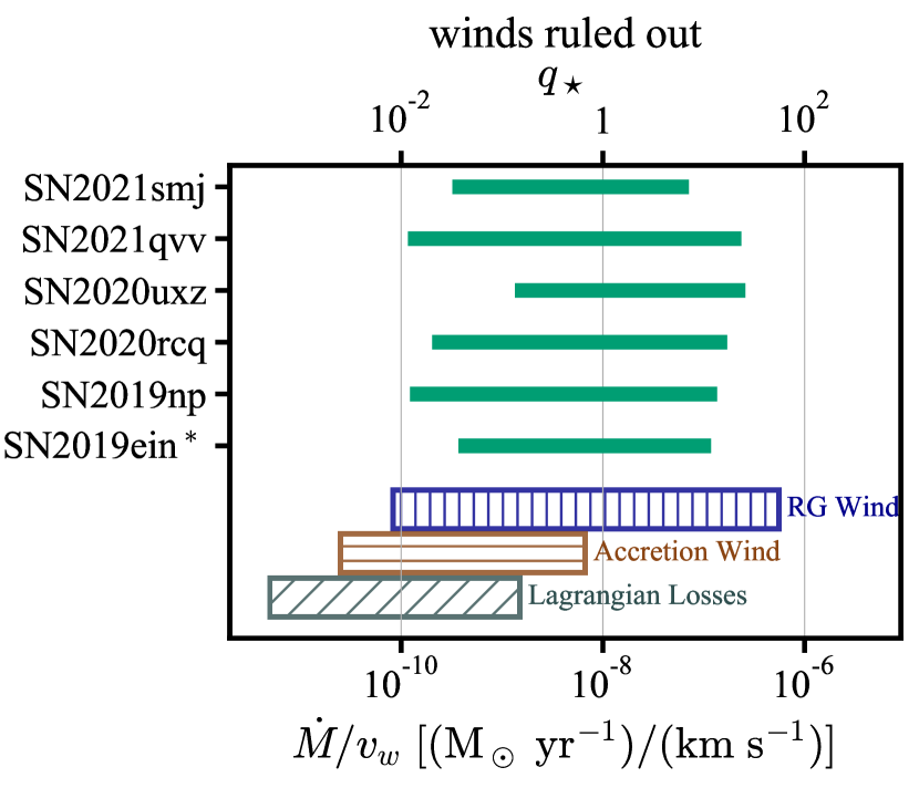
Using a grid of light curves varying $q_{\star}$, we are able to determine which winds our radio limits could detect. The span of wind densities thus ruled out is shown in Figure 3. The low-density edge to these limits comes from the early-time and low-luminosity peaks of low-$q_{\star}$ light curves. The high-density edge is due to the late-time peak of high-$q_{\star}$ light curves that results from free-free absorption.

We see that for most SNe, we are able to rule out winds down to densities $\dot{M}/v_{w}\sim 10^{-9}-10^{-10}~{}\mathrm{(M_{\odot}~{}yr^{-1})/(km~{}s^{-1})}$. This represents a ruling out of the lowest density symbiotic winds, and it also rules out a significant span of the possible winds associated with high accretion rates.

Figure 3: Solid green bars show the span of winds ruled out by radio observations, assuming fiducial shock parameters – lower and higher density winds are allowed. Hatched regions show expectations for wind densities from the physical mechanisms discussed in the text.

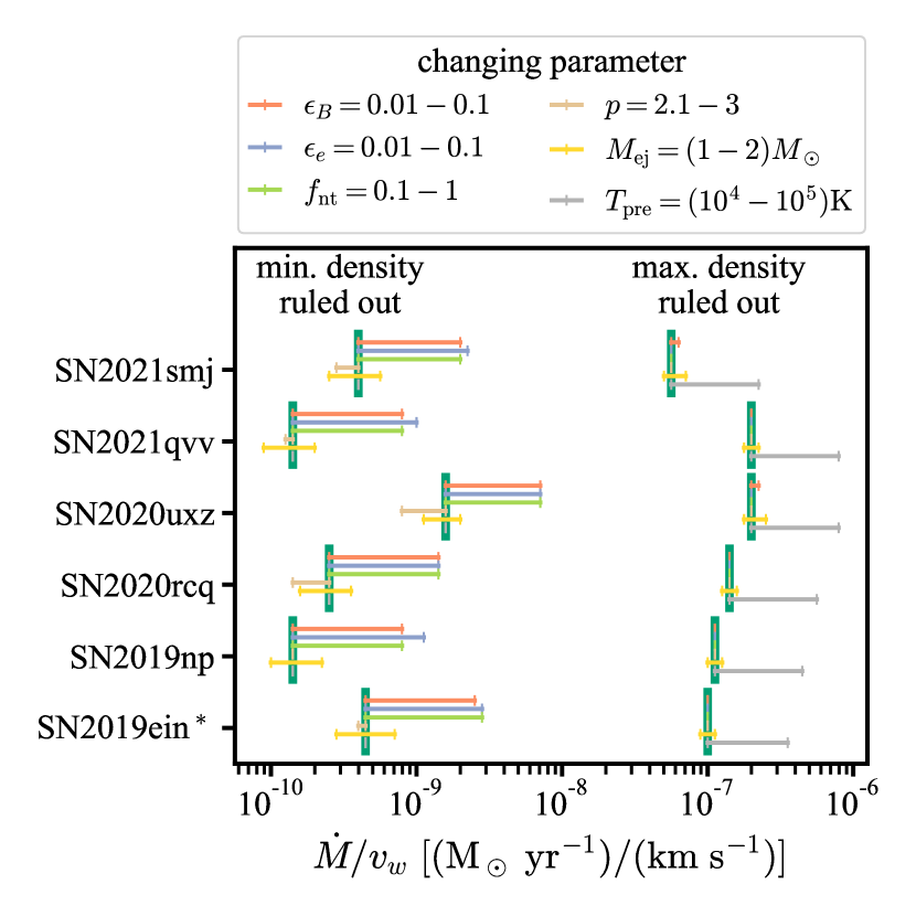
However, as discussed in § 3, these constraints are subject to underlying uncertainties. Our default values for various model parameters (e.g., $\epsilon_{B}$) were chosen to reflect values that are commonly used in the literature of SNe interacting with winds. In Figure 4 we show how changing each parameter affects the constraint for each of our targets. A decade (“1 dex”) decrease in $\epsilon_{B}$, $\epsilon_{e}$, or $f_{\mathrm{nt}}$ results in a $\sim 0.8$ dex increase on the minimum wind density we can rule out, weakening the constraining power of the observations. On the other end, we see that a 1 dex increase in the absorbing (pre-shock) CSM temperature, $T_{\mathrm{pre}}$, increases the window of CSM ruled out by $\sim 0.5$ dex. Smaller effects are seen when changing the power-law slope of the non-thermal electrons ($p$) or the ejecta mass, since these parameters do not suffer orders of magnitude uncertainty in their values. We see that if $p=2.1$, our observations can rule out slightly lower density winds in some cases. For ejecta mass, we consider decreasing from $1.38~{}M_{\odot}$ to $1~{}M_{\odot}$ (sub-Chandrasekhar explosion, ) as well as increasing to $2~{}M_{\odot}$ (super-Chandrasekhar explosion), and we see that this has a small impact on the lowest density wind that we can constrain.

Furthermore, we investigated the effect of the assumed distance on our wind density limits, by re-analyzing the radio data with redshift-independent distances from the NASA/IPAC Extragalactic Database for SNe 2019np (Willick et al., 1997; Theureau et al., 2007; Sorce et al., 2014), 2020uxz (Tully et al., 2009, 2013, 2016; Springob et al., 2009), and 2021qvv (Jordán et al., 2005, 2007; Villegas et al., 2010) and the error range on the distance to SN 2019ein given in ¡ Pellegrino et al. (2020). For SNe 2019ein and 2021qvv, the distance differences are $<0.1~{}\mathrm{dex}$, whereas the distance varies more for SN 2019np and SN 2020uxz ($\lesssim 0.3~{}\mathrm{dex}$ and $\lesssim 0.15~{}\mathrm{dex}$, respectively). The resulting variation in the minimum density constrained is of a similar magnitude. Therefore, we conclude that distance uncertainty is subdominant to the uncertainties from underlying physics.

For the purposes of ruling out low density winds around SNe Ia, it is clear that the uncertainties in $\epsilon_{B}$, $\epsilon_{e}$, and $f_{\mathrm{nt}}$ are key issues. Considering that the true values could be even lower than what we chose for our illustration, and that their effects compound, it is easy to see a pessimistic combination that renders the radio observations totally unconstraining. As sensitive radio data are already in hand from this and other studies, we therefore emphasize the great importance of research, especially theoretical work, on magnetic field amplification and electron acceleration in SN shocks.

Figure 4: The effect of model parameter assumptions on our results for the wind model. Vertical green bars indicate the minimum and maximum wind density ruled out under our “fiducial” assumptions (see Figure 3). Horizontal error bars on these show the effect of changing the magnetic field energy density ($\epsilon_{B}$, red), nonrelativistic electron energy density ($\epsilon_{e}$, blue), fraction of electrons in the power-law population ($f_{\mathrm{nt}}$, green), power-law index of the relativistic electrons ($p$, brown), supernova ejecta mass ($M_{\mathrm{ej}}$, yellow), and temperature of the preshock CSM ($T_{\mathrm{pre}}$, grey). See text for description of the effect of distance uncertainty.

4.1.1 Higher-Density Winds Disfavored by Optical Data

Looking at the $g$- and $r$-band optical light curves from the Zwicky Transient Facility via the ALeRCE ZTF Explorer and the optical spectra on the Transient Name Server, we see no obvious indication of interaction with high-density material for our six targets, which can show up in several ways. Considering extended winds, we can use this to complement the radio limits on wind density on the high-$q_{\star}$ side. From Ofek et al. (2013), the fact that CSM would affect the rise time limits the mass loss rate to $<2.7\times 10^{-4}~{}\mathrm{(M_{\odot}~{}yr^{-1})/(km~{}s^{-1})}$. Narrow H$\alpha$ line formation from recombination is created at the level of $\sim 5\times 10^{39}~{}\mathrm{erg~{}s^{-1}}$ for $\dot{M}/v_{w}=10^{-5}~{}\mathrm{(M_{\odot}~{}yr^{-1})/(km~{}s^{-1})}$, which is approximately where free-free absorption cuts off the utility of the early-time radio limits. Densities higher than this would have a more dramatic effect – Silverman et al. (2013) estimate that SNe Ia-CSM have $\dot{M}/v_{w}=10^{-3}~{}\mathrm{(M_{\odot}~{}yr^{-1})/(km~{}s^{-1})}$, and in those cases there is a very strong continuum in the optical spectra in addition to the narrow and broad H$\alpha$ emission features. There is no obvious indication of any of these features in the optical data, disfavoring the possibility that there is CSM more dense than the range we are able to rule out with our radio observations. However, a more in-depth analysis of the optical data would be necessary for a definitive conclusion – for example, only after constructing a bolometric light curve do Sai et al. (2022) see a low-level (5%) excess in one of our targets, SN 2019np. In the case of SN 2019np, Sai et al. (2022) present spectra at very early times that show no evidence of CSM interaction emission, and their analysis indicates that this small excess is caused by an extended ⁵⁶Ni distribution in the ejecta.

4.1.2 Prior Limits on Wind Scenarios

Chomiuk et al. (2016) and Lundqvist et al. (2020) present the collected radio observations of SNe Ia from the literature (see references therein), and Hosseinzadeh et al. (2022) provides an additional case with SN 2021aefx. SN 2021aefx is an early-excess SN Ia, but the radio observations at $t\gtrsim 4~{}\mathrm{days}$ post-explosion probe an extended medium rather than possible compact CSM so we interpret these observations in a wind-like CSM context, as do Hosseinzadeh et al. (2022) – see also § 4.2. We apply the same methodology to these collected datasets as to our new observations to discuss the impact of our six new SNe Ia to our overall understanding of SN Ia progenitors. Here we confine ourselves to the normal, 91T-like (“shallow Silicon”), and 91bg-like (“cool”) SNe Ia from Chomiuk et al. (2016).

Figure 5 shows the result of this analysis as a histogram of how many SNe Ia are known with radio data that can constrain winds of different densities, with a focus on the lowest densities. We indicate how many of the SNe Ia at each density come from our sample, the literature sample of SNe Ia with observations within 10 days post-explosion, and the full literature sample (including SNe Ia first observed later than 10 days post-explosion) for an analysis with our fiducial parameter set. For the full sample, we also indicate how the histogram may shift with different choices of parameters, as in Figure 3. Note that the two events at the very lowest densities are SN 2011fe and SN 2014J (Chomiuk et al., 2012; Pérez-Torres et al., 2014).

We show by this plot that the six SNe Ia presented in this manuscript represent a significant increase in the number of SNe Ia with constraints at these low wind densities. Again, this is because interaction with low-density winds creates a radio light curve that peaks at early times (see Figure 2). The relative impact of our observations increases as one looks to lower density constraints – the sample nearly doubles events that can constrain the accretion wind and Lagrangian losses scenarios. The predominance of SNe Ia with early-time observations at the lowest density end of this histogram highlights the necessity of rapid follow-up observations, particularly if it turns out that the microphysics of the shock acceleration and magnetic field amplification is unfavorable (i.e., the weakest limits are correct).

Figure 5: A cumulative histogram of how many SNe Ia can rule out low-density winds, comparing this paper (green filled) to published SNe Ia with radio observations within 10 days (green hatched) and the full sample of all published SN Ia radio observations (green solid line). Our observations represent a significant increase to the number of SNe Ia that can rule out winds with $q_{\star}<0.1$.

4.2 Compact CSM Shells

Recall from § 3.3.1 that our hope for radio emission in the case of compact shell interaction is that after the shock has swept over the CSM, the last, small parcel of gas may be accelerated so rapidly that its cooling time rapidly increases and relativistic electrons can survive. We now assess this possibility with our SNEC simulation.

Using the method described in §3.3.1, we calculate cooling time for $\gamma$ corresponding to 6 GHz; however, we find that while the shock is in the CSM, the energy density is so high that $B\gtrsim 10^{3}~{}\mathrm{G}$ and $\nu_{\mathrm{cyc}}\gtrsim 10~{}\mathrm{GHz}$ ($\nu_{\mathrm{cyc}}\sim 3B~{}\mathrm{MHz}$). Physically, this means that even without cooling and with $\epsilon_{B}=0.003$, synchrotron emission would not extend down to 6 GHz until the energy density drops after shock breakout. In our calculation of the cooling time, we use $\gamma=1$ when $\nu_{\mathrm{cyc}}>6~{}\mathrm{GHz}$.

Figure 6 shows the cooling efficiency of relativistic electrons over time immediately behind the shock front in the SNEC simulation. We indicate the time that the shock front overtakes the outer edge of the CSM ($R_{f}=R_{\mathrm{out}}$), and reiterate that we do not expect 6 GHz emission prior to this point due to high $\nu_{\mathrm{cyc}}$. Prior to this point, we see that cooling is extremely efficient, although it is trending to longer cooling times. After the shock crosses the CSM, the cooling time does, indeed, increase very rapidly. However, it remains very short compared to the hydrodynamic time. Cooling times are longer for the lower $\epsilon_{B}$, because the power radiated by synchrotron emission is lower and – once the shock has crossed the CSM – $\gamma$ is also lower. Yet even in the lower $\epsilon_{B}$ case, the situation looks grim for relativistic electron survival.

Figure 6: The cooling time of relativistic electrons that produce 6 GHz emission compared to the hydrodynamic timescale (i.e., the efficiency of relativistic electron cooling) as a function of time, assuming $\epsilon_{B}=0.1$ (solid) and $\epsilon_{B}=0.003$ (dashed). $R_{f}=R_{\mathrm{out}}$ marks the time the shock crosses the compact CSM shell. We see that cooling of the relativistic electrons is likely too efficient for relativistic electrons to survive despite the rapid expansion of the CSM after the interaction.

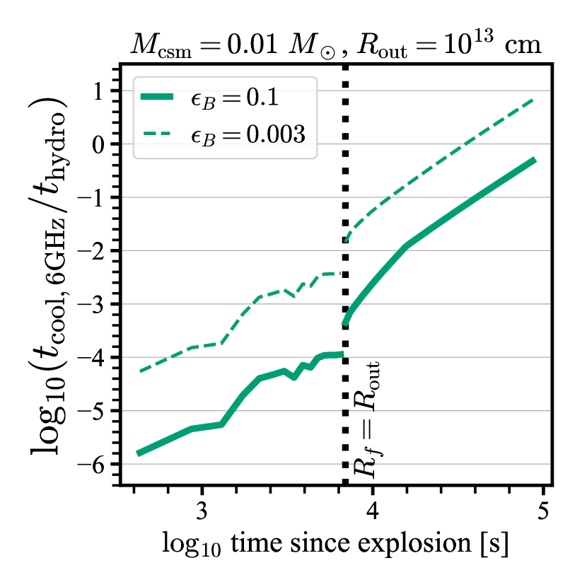
For a variety of reasons, we determine that interaction with compact shells is unlikely to produce detectable radio emission from the synchrotron process. Prior to the shock crossing the CSM, free-free absorption will stifle radio emission and cooling will severely limit the volume of relativistic electrons; furthermore, we have seen that the magnetic field strength may be so high that synchrotron emission is pushed to frequencies above the radio range. Once the shock crosses the CSM, our hope was that the rapid rarification of the outermost CSM, and thus increase of cooling time, might preserve a small fraction of relativistic electrons. However, it seems from our estimates that the cooling time does not increase fast enough to preserve the relativistic population, though the issue with the magnetic field strength is resolved such that there could be synchrotron emission at radio frequencies.

It may be worth determining in future work whether the X-rays generated from cooling relativistic electrons can at any point escape the envelope, producing a complementary X-ray/gamma-ray flash to the optical/UV excess, analogous to the shock breakout from core-collapse SNe (Nakar & Sari, 2010), which could potentially leverage the rapid follow-up capabilities of a space telescope like the Neil Gehrels Swift Observatory. A thermal X-ray signal is not expected from our models because the shock-heated gas, equilibrating with the radiation field, reaches only $kT\sim 0.01~{}\mathrm{keV}$. We mention this to contrast with the case of the calcium-strong transient SN 2019ehk – Jacobson-Galán et al. (2020) interpret the Swift X-ray detection of SN 2019ehk in the context of interaction with a compact shell, but attribute the X-ray emission to thermal emission from $kT>10~{}\mathrm{keV}$ gas. The emission from cooling high-energy electrons would be non-thermal and of much shorter duration.

Finally, we note that the radio prospects may not be not entirely hopeless, despite our simulation result. In the first place, we have not performed a detailed particle-in-cell simulation that tracks the evolution of the ion and electron populations as they interact with each other and the magnetic field. Such a simulation would need to also include the effects of radiative cooling and photon trapping in this dense environment, and therefore represents a significant research project outside the scope of the current work. However, even if such a calculation confirmed our own, there are some remaining potential avenues for radio emission in the compact shell scenario: where the CSM is aspherical, perhaps the ejecta interact with significantly lower-density CSM in some fraction of the volume, or, if there is a low-density wind outside the compact shell, radio emission could arise from the interaction with this wind. Indeed, for the case of SN 2021aefx, the analyses of both Hosseinzadeh et al. (2022) and this work are focused on constraining the presence of an extended medium outside a possible compact shell. Further work predicting the environment out to $r\sim 10^{16}~{}\mathrm{cm}$ and assessing how initial interaction with a dense shell would change the density and velocity profile of the fast ejecta as it propagates into an extended medium are needed to assess these possibilities.

5 Summary

In this paper, we have presented Jansky VLA 6 GHz observations within 10 days post-explosion for six SNe Ia with the goal of constraining Type Ia supernova progenitors via their circumstellar environments.

The nature of the mass-donor companion that ignites CO WDs as SNe Ia remains a mystery, despite decades of effort. Whether mass donation happens via accretion or merger, whether explosion occurs at the center or surface, whether the companion is degenerate, are all matters of debate – and each possibility may be at play to create a tapestry of progenitor scenarios whose relative contributions are to be accounted.

Characterizing the circumstellar environments of SNe Ia can help to shed light on these questions because different progenitor scenarios create different environments in the millennia leading up to explosion. In this paper, we were particularly interested in low-density winds from accretion scenarios that would leave no optical signature and the compact shells of WD merger scenarios that may create observed early-time optical excesses in SN Ia light curves. In the first case, radio observations are one of the only ways to see the CSM; in the second case, a radio signal would be a clear tie to non-thermal electron populations characteristic of shocks to clarify the origin of the emission.

Our observations can constrain the lowest density winds from red giant companions, optically thick accretion winds, and the loss of material from the outer Lagrangian point of the disk (§ 3.1, 4.1). To analyze the observations in this context, we employ the self-similar model of Chevalier (1982a), which works well for extended winds (Figures 1 & 2). With standard (fiducial) assumptions about synchrotron emission, the observations rule out winds down to $(10^{-9}-10^{-10})~{}\mathrm{M_{\odot}~{}yr^{-1}/(km~{}s^{-1})}$, depending on the target, which represents the lowest density red giant winds and a large portion of possible accretion winds (Figure 3). In our analysis we have accounted for uncertainties in the microphysics of magnetic field amplification and electron energy distribution that affect the low-density limit (Figure 4). Densities above $\sim 10^{-7}~{}\mathrm{M_{\odot}~{}yr^{-1}/(km~{}s^{-1})}$ are not ruled out by the radio observations of these targets, but are disfavored by the lack of optical signatures of interaction. These six events represent a substantial increase in the number of SNe Ia with radio observations with such low density limits (Figure 5).

Toward the aim of understanding the origin of early-time excess in the optical/UV light curves of some SNe Ia, we have assessed the possibility of radio observations detecting shock emission from the interaction of SN Ia ejecta with a dense CSM truncated at $R_{\mathrm{out}}=10^{13}~{}\mathrm{cm}$ (§ 3.2, 4.2). CSM masses between $(0.01-0.1)~{}M_{\odot}$ have been suggested for creating the optical/UV excesses, and through analytic calculations we have shown that such masses require radiation hydrodynamics simulations to calculate the evolution of the shock wave and that radio emission will be severely affected by the cooling of relativistic electrons in the dense gas (Figure 1, § 3). To assess the possibility that the rapid rarefication of the CSM after the shock has swept over the CSM could dramatically increase the cooling time of electrons and allow some to survive and produce radio emission, we have performed radiation hydrodynamic calculations with SNEC. Our model of a $0.01~{}M_{\odot}$ shell extending to $10^{13}~{}\mathrm{cm}$ is an expansion of the model suite presented in Piro & Morozova (2016) to a larger radius and lower CSM mass. This model has the same CSM as in the simulation by Jiang et al. (2021) to reproduce the early excess of SN 2020hvf, but we assume typical SN Ia explosion parameters whereas their simulation had higher-mass ejecta than normal. We find that the relativistic electron cooling time remains very short even through the rarefaction phase, and we therefore do not expect the compact shell interaction scenario to produce radio emission at any phase. There may, perhaps, be an X-ray flare from the cooling relativistic electrons at the very end of interaction. If the WD merger or accretion from a WD scenarios produce a more extended and less dense circumstellar environment, it may be possible for radio emission to be produced from interaction with this more extended medium.

Overall, we see that our deep, early-time observations serve to probe the existence of low-density winds around SNe Ia, even accounting for uncertainties in the underlying physics of magnetic field amplification. With these observations we significantly increase the sample of observations that can constrain not only red giant winds, but the lower density accretion winds from high accretion rates in Roche lobe overflow. Detailed tracking of the shock evolution through a high density, compact CSM reveals that relativistic electrons cannot survive to produce synchrotron emission. This is unfortunate, because such emission would unambiguously indicate the presence of a shock in SNe Ia with short-duration optical/UV excess to determine the physical origin of this emission.

References

- Abbott et al. (2019) Abbott, T. M. C., Allam, S., Andersen, P., et al. 2019, ApJ, 872, L30
- Ashall et al. (2022) Ashall, C., Lu, J., Shappee, B. J., et al. 2022, arXiv e-prints, arXiv:2205.00606
- Astropy Collaboration et al. (2013) Astropy Collaboration, Robitaille, T. P., Tollerud, E. J., et al. 2013, A&A, 558, A33
- Björnsson & Fransson (2004) Björnsson, C.-I., & Fransson, C. 2004, ApJ, 605, 823
- Bloom et al. (2012) Bloom, J. S., Kasen, D., Shen, K. J., et al. 2012, ApJ, 744, L17
- Bochenek et al. (2018) Bochenek, C. D., Dwarkadas, V. V., Silverman, J. M., et al. 2018, MNRAS, 473, 336
- Branch (1998) Branch, D. 1998, ARA&A, 36, 17
- Branch et al. (1995) Branch, D., Livio, M., Yungelson, L. R., Boffi, F. R., & Baron, E. 1995, PASP, 107, 1019
- Cao et al. (2015) Cao, Y., Kulkarni, S. R., Howell, D. A., et al. 2015, Nature, 521, 328, doi: 10.1038/nature14440
- Caprioli & Spitkovsky (2014) Caprioli, D., & Spitkovsky, A. 2014, ApJ, 783, 91, doi: 10.1088/0004-637X/783/2/91
- Chevalier (1982a) Chevalier, R. A. 1982a, ApJ, 258, 790, doi: 10.1086/160126
- Chevalier (1982b) —. 1982b, ApJ, 259, 302
- Chevalier (1998) —. 1998, ApJ, 499, 810, doi: 10.1086/305676
- Chevalier & Fransson (1994) Chevalier, R. A., & Fransson, C. 1994, ApJ, 420, 268, doi: 10.1086/173557
- Chevalier & Fransson (2006) —. 2006, ApJ, 651, 381, doi: 10.1086/507606
- Chevalier et al. (2004) Chevalier, R. A., Li, Z.-Y., & Fransson, C. 2004, ApJ, 606, 369, doi: 10.1086/382867
- Chomiuk & Wilcots (2009) Chomiuk, L., & Wilcots, E. M. 2009, ApJ, 703, 370, doi: 10.1088/0004-637X/703/1/370
- Chomiuk et al. (2012) Chomiuk, L., Soderberg, A. M., Moe, M., et al. 2012, ApJ, 750, 164, doi: 10.1088/0004-637X/750/2/164
- Chomiuk et al. (2016) Chomiuk, L., Soderberg, A. M., Chevalier, R. A., et al. 2016, ApJ, 821, 119, doi: 10.3847/0004-637X/821/2/119
- Churazov et al. (2015) Churazov, E., Sunyaev, R., Isern, J., et al. 2015, ApJ, 812, 62
- Crumley et al. (2019) Crumley, P., Caprioli, D., Markoff, S., & Spitkovsky, A. 2019, MNRAS, 485, 5105, doi: 10.1093/mnras/stz232
- Deckers et al. (2022) Deckers, M., Maguire, K., Magee, M. R., et al. 2022, arXiv e-prints, arXiv:2202.12914
- Diesing & Caprioli (2021) Diesing, R., & Caprioli, D. 2021, ApJ, 922, 1
- Duffell & Kasen (2017) Duffell, P. C., & Kasen, D. 2017, ApJ, 842, 18
- Freedman et al. (2019) Freedman, W. L., Madore, B. F., Hatt, D., et al. 2019, ApJ, 882, 34
- Green (2019) Green, D. A. 2019, Journal of Astrophysics and Astronomy, 40, 36, doi: 10.1007/s12036-019-9601-6
- Hachisu et al. (1996) Hachisu, I., Kato, M., & Nomoto, K. 1996, ApJ, 470, L97
- Hachisu et al. (1999) Hachisu, I., Kato, M., Nomoto, K., & Umeda, H. 1999, ApJ, 519, 314
- Hamuy et al. (2003) Hamuy, M., Phillips, M. M., Suntzeff, N. B., et al. 2003, Nature, 424, 651, doi: 10.1038/nature01854
- Harris et al. (2016) Harris, C. E., Nugent, P. E., & Kasen, D. N. 2016, ApJ, 823, 100, doi: 10.3847/0004-637X/823/2/100
- Horesh et al. (2013) Horesh, A., Stockdale, C., Fox, D. B., et al. 2013, MNRAS, 436, 1258
- Hosseinzadeh et al. (2017) Hosseinzadeh, G., Sand, D. J., Valenti, S., et al. 2017, ApJ, 845, L11, doi: 10.3847/2041-8213/aa8402
- Hosseinzadeh et al. (2022) Hosseinzadeh, G., Sand, D. J., Lundqvist, P., et al. 2022, arXiv e-prints, arXiv:2205.02236
- Huang & Yu (1996) Huang, R.-q., & Yu, K. N. 1996, Chinese Astron. Astrophys., 20, 175
- Hunter (2007) Hunter, J. D. 2007, Computing in Science & Engineering, 9, 90
- Iben & Tutukov (1984) Iben, I., J., & Tutukov, A. V. 1984, ApJS, 54, 335
- Jacobson-Galán et al. (2020) Jacobson-Galán, W. V., Margutti, R., Kilpatrick, C. D., et al. 2020, ApJ, 898, 166
- Jiang et al. (2021) Jiang, J.-a., Maeda, K., Kawabata, M., et al. 2021, ApJ, 923, L8
- Jones et al. (2001) Jones, E., Oliphant, T., Peterson, P., et al. 2001, SciPy: Open source scientific tools for Python
- Jordán et al. (2005) Jordán, A., Côté, P., Blakeslee, J. P., et al. 2005, ApJ, 634, 1002, doi: 10.1086/497092
- Jordán et al. (2007) Jordán, A., McLaughlin, D. E., Côté, P., et al. 2007, ApJS, 171, 101, doi: 10.1086/516840
- Kasen (2010) Kasen, D. 2010, ApJ, 708, 1025, doi: 10.1088/0004-637X/708/2/1025
- Li et al. (2011) Li, W., Bloom, J. S., Podsiadlowski, P., et al. 2011, Nature, 480, 348
- Livio & Mazzali (2018) Livio, M., & Mazzali, P. 2018, Phys. Rep., 736, 1
- Lundqvist et al. (2020) Lundqvist, P., Kundu, E., Pérez-Torres, M. A., et al. 2020, ApJ, 890, 159
- Macaulay et al. (2019) Macaulay, E., Nichol, R. C., Bacon, D., et al. 2019, MNRAS, 486, 2184
- Magee & Maguire (2020) Magee, M. R., & Maguire, K. 2020, A&A, 642, A189, doi: 10.1051/0004-6361/202037870
- Maoz et al. (2014) Maoz, D., Mannucci, F., & Nelemans, G. 2014, ARA&A, 52, 107
- Marcowith et al. (2020) Marcowith, A., Ferrand, G., Grech, M., et al. 2020, Living Reviews in Computational Astrophysics, 6, 1, doi: 10.1007/s41115-020-0007-6
- Margutti et al. (2014) Margutti, R., Parrent, J., Kamble, A., et al. 2014, ApJ, 790, 52
- Margutti et al. (2012) Margutti, R., Soderberg, A. M., Chomiuk, L., et al. 2012, ApJ, 751, 134
- Marion et al. (2016) Marion, G. H., Brown, P. J., Vinkó, J., et al. 2016, ApJ, 820, 92, doi: 10.3847/0004-637X/820/2/92
- Marongiu et al. (2022) Marongiu, M., Guidorzi, C., Stratta, G., et al. 2022, A&A, 658, A11
- McCully et al. (2014) McCully, C., Jha, S. W., Foley, R. J., et al. 2014, Nature, 512, 54
- Miller et al. (2018) Miller, A. A., Cao, Y., Piro, A. L., et al. 2018, ApJ, 852, 100, doi: 10.3847/1538-4357/aaa01f
- Moore & Bildsten (2012) Moore, K., & Bildsten, L. 2012, ApJ, 761, 182, doi: 10.1088/0004-637X/761/2/182
- Morozova et al. (2015) Morozova, V., Piro, A. L., Renzo, M., et al. 2015, ApJ, 814, 63
- Nakar & Sari (2010) Nakar, E., & Sari, R. 2010, ApJ, 725, 904
- Ofek et al. (2013) Ofek, E. O., Lin, L., Kouveliotou, C., et al. 2013, ApJ, 768, 47
- Oliphant (2006) Oliphant, T. 2006, A guide to NumPy (USA: Trelgol Publishing)
- Pakmor et al. (2012) Pakmor, R., Kromer, M., Taubenberger, S., et al. 2012, ApJ, 747, L10, doi: 10.1088/2041-8205/747/1/L10
- Panaitescu & Kumar (2002) Panaitescu, A., & Kumar, P. 2002, ApJ, 571, 779
- Paxton et al. (2011) Paxton, B., Bildsten, L., Dotter, A., et al. 2011, ApJS, 192, 3
- Pellegrino et al. (2020) Pellegrino, C., Howell, D. A., Sarbadhicary, S. K., et al. 2020, ApJ, 897, 159, doi: 10.3847/1538-4357/ab8e3f
- Pérez-Torres et al. (2014) Pérez-Torres, M. A., Lundqvist, P., Beswick, R. J., et al. 2014, ApJ, 792, 38
- Piro & Morozova (2016) Piro, A. L., & Morozova, V. S. 2016, ApJ, 826, 96
- Polin et al. (2019) Polin, A., Nugent, P., & Kasen, D. 2019, ApJ, 873, 84, doi: 10.3847/1538-4357/aafb6a
- Raskin & Kasen (2013) Raskin, C., & Kasen, D. 2013, ApJ, 772, 1, doi: 10.1088/0004-637X/772/1/1
- Reynolds et al. (2021) Reynolds, S. P., Williams, B. J., Borkowski, K. J., & Long, K. S. 2021, ApJ, 917, 55, doi: 10.3847/1538-4357/ac0ced
- Riess et al. (2016) Riess, A. G., Macri, L. M., Hoffmann, S. L., et al. 2016, ApJ, 826, 56
- Sai et al. (2022) Sai, H., Wang, X., Elias-Rosa, N., et al. 2022, arXiv e-prints, arXiv:2205.15596
- Schwab et al. (2012) Schwab, J., Shen, K. J., Quataert, E., Dan, M., & Rosswog, S. 2012, MNRAS, 427, 190
- Seaquist & Taylor (1990) Seaquist, E. R., & Taylor, A. R. 1990, ApJ, 349, 313, doi: 10.1086/168315
- Shen & Bildsten (2007) Shen, K. J., & Bildsten, L. 2007, ApJ, 660, 1444
- Shen et al. (2012) Shen, K. J., Bildsten, L., Kasen, D., & Quataert, E. 2012, ApJ, 748, 35
- Silverman et al. (2013) Silverman, J. M., Nugent, P. E., Gal-Yam, A., et al. 2013, ApJS, 207, 3
- Soderberg et al. (2005) Soderberg, A. M., Kulkarni, S. R., Berger, E., et al. 2005, ApJ, 621, 908
- Soker (2013) Soker, N. 2013, in IAU Symposium, Vol. 281, Binary Paths to Type Ia Supernovae Explosions, ed. R. Di Stefano, M. Orio, & M. Moe, 72–75, doi: 10.1017/S174392131201472X
- Sorce et al. (2014) Sorce, J. G., Tully, R. B., Courtois, H. M., et al. 2014, MNRAS, 444, 527, doi: 10.1093/mnras/stu1450
- Springob et al. (2009) Springob, C. M., Masters, K. L., Haynes, M. P., Giovanelli, R., & Marinoni, C. 2009, ApJS, 182, 474, doi: 10.1088/0067-0049/182/1/474
- Theureau et al. (2007) Theureau, G., Hanski, M. O., Coudreau, N., Hallet, N., & Martin, J. M. 2007, A&A, 465, 71, doi: 10.1051/0004-6361:20066187
- Tully et al. (2016) Tully, R. B., Courtois, H. M., & Sorce, J. G. 2016, AJ, 152, 50, doi: 10.3847/0004-6256/152/2/50
- Tully et al. (2009) Tully, R. B., Rizzi, L., Shaya, E. J., et al. 2009, AJ, 138, 323, doi: 10.1088/0004-6256/138/2/323
- Tully et al. (2013) Tully, R. B., Courtois, H. M., Dolphin, A. E., et al. 2013, AJ, 146, 86, doi: 10.1088/0004-6256/146/4/86
- Villegas et al. (2010) Villegas, D., Jordán, A., Peng, E. W., et al. 2010, ApJ, 717, 603, doi: 10.1088/0004-637X/717/2/603
- Weiler et al. (1986) Weiler, K. W., Sramek, R. A., Panagia, N., van der Hulst, J. M., & Salvati, M. 1986, ApJ, 301, 790
- Whelan & Iben (1973) Whelan, J., & Iben, Icko, J. 1973, ApJ, 186, 1007
- Willick et al. (1997) Willick, J. A., Courteau, S., Faber, S. M., et al. 1997, ApJS, 109, 333, doi: 10.1086/312983
- Wright (2006) Wright, E. L. 2006, PASP, 118, 1711, doi: 10.1086/510102
- Yost et al. (2003) Yost, S. A., Harrison, F. A., Sari, R., & Frail, D. A. 2003, ApJ, 597, 459, doi: 10.1086/378288