Steady-state quantum chaos in open quantum systems

Abstract

We introduce the notion of steady-state quantum chaos as a general phenomenon in open quantum many-body systems. Classifying an isolated or open quantum system as integrable or chaotic relies in general on the properties of the equations governing its time evolution. This however may fail in predicting the actual nature of the quantum dynamics, that can be either regular or chaotic depending on the initial state. Chaos and integrability in the steady state of an open quantum system are instead uniquely determined by the spectral structure of the time evolution generator. To characterize steady-state quantum chaos we introduce a spectral analysis based on the spectral statistics of quantum trajectories (SSQT). We test the generality and reliability of the SSQT criterion on several dissipative systems, further showing that an open system with chaotic structure can evolve towards either a chaotic or integrable steady state. We study steady-state chaos in the driven-dissipative Bose-Hubbard model, a paradigmatic example of out-of-equilibrium bosonic system without particle number conservation. This system is widely employed as a building block in state-of-the-art noisy intermediate-scale quantum devices, with applications in quantum computation and sensing. Finally, our analysis shows the existence of an emergent dissipative quantum chaos, where the classical and semi-classical limits display an integrable behaviour. This emergent dissipative quantum chaos arises from the quantum and classical fluctuations associated with the dissipation mechanism. Our work establishes a fundamental understanding of the integrable and chaotic dynamics of open quantum systems and paves the way for the investigation of dissipative quantum chaos and its consequences on quantum technologies.

I Introduction

The study of chaos and integrability in open quantum many-body systems is central in many research areas ranging from high-energy physics to condensed matter, quantum optics, and quantum technologies. In an open quantum system, the degrees of freedom of the system are coupled to those of the surrounding environment, resulting in effective system dynamics that departs significantly from the paradigm of unitary quantum mechanics [1, 2]. The properties of open quantum systems have long been used for the preparation and stabilization of quantum states, with both fundamental [3, 4, 5, 6] and technological [7, 8, 9, 10, 11] purposes. Progress in this field includes the theoretical and experimental study of dissipative phase transitions [12, 13, 14, 15, 16, 17, 18, 19, 20, 21, 22], the development of protocols for error correction and suppression [23, 24, 25, 26, 27, 28, 29], the stabilization and control of entangled, topological and localized phases [30, 31, 32, 33, 34, 35], the characterization of dissipative quantum chaos (DQC) [36, 37, 38, 39, 40, 41, 42, 43, 44, 45, 46, 47, 48, 49, 50, 51, 52, 53].

Most of complex many-body quantum systems are expected to be chaotic. Quantum chaos, both in isolated and open systems, is usually characterized by comparing the spectral properties of the time evolution generator to the universal predictions of random matrix theory, within a framework known as the quantum chaos conjecture [54, 55]. To date, general criteria for probing DQC have been developed [40], and symmetry-based systematic classifications of DQC have been elaborated [39, 47, 51, 50].

A classification of integrability or chaos based uniquely on spectral properties, however, is likely to fail in predicting the actual nature of the quantum dynamics. For instance, in isolated systems, the dynamics can be either regular or chaotic depending on the initial state. The same difficulty persists when considering open quantum systems described by, e.g., a Lindblad master equation [56, 1]. In this case, ever since the pioneering work of Grobe, Haake, and Sommers [57], DQC has been treated as an inherently transient feature manifesting before the system reaches its steady state, i.e., a density matrix that is asymptotically stationary [1].

In this work we show that it is possible to provide an operational definition of quantum chaos in the steady state of an open quantum system. This definition lifts the arbitrariness discussed above and establishes a general understanding of the chaotic and integrable properties of Lindbladian dynamics. Under quite reasonable assumptions, the dynamics of an open system irreversibly evolves towards a unique steady state . Differently from Hamiltonian dynamics, or any kind of transient dynamics, in the steady state the information about the initial condition is lost. The properties of any unique steady-state, therefore, depend only on the structure of the master equation. Even so, defining the chaotic or integrable nature of a state that does not evolve in time seems contradictory. Attempts at such a characterization have been proposed, based on the analysis of the entanglement Hamiltonian or the out-of-time-order correlators [41, 42, 49, 44]. We will show that these approaches, and more in general spectral criteria, can provide ambiguous answers, and a rigorous characterization of integrability and chaos in the steady state of an open quantum system remains a major theoretical challenge.

Our work overcomes these ambiguities and fills the gap by defining steady-state quantum chaos through a combination of dynamical and steady-state properties. This is our first result. As we will show, the notion of steady-state chaos is justified by considering the stationary density matrix as the average over a statistical ensemble of single dynamical realizations (stochastic quantum trajectories) [59, 60, 61, 62]. Specifically, we introduce the spectral statistics of quantum trajectories (SSQT) as a criterion able to identify chaotic or integrable dynamics in the steady state of an open quantum system, based on the universal predictions of random matrix theory and on the stochastic dynamics of single quantum trajectories. This approach leads to a rigorous and model-independent definition of steady-state quantum chaos as a general phenomenon in open quantum systems. Interestingly, we find that driven-dissipative systems with chaotic spectral structure, can evolve towards either regular of chaotic steady states. When applied to the transient dynamics, the SSQT criterion includes the transient DQC described, for example, in Refs. [36, 40, 47, 51]. In this case, the choice of the initial state matters in defining quantum dynamics as integrable or chaotic.

The second result of this work is the investigation of steady-state and transient quantum chaos in driven-dissipative Bose-Hubbard systems. Driven-dissipative systems of coupled nonlinear bosonic oscillators are the focus of intense investigations, as they provide a realistic model for several quantum technology platforms [63, 64, 65], such as superconducting circuits [66, 67], semiconductor artificial structures [68, 69], optomechanical resonators [70], and trapped ions [71, 72]. These systems have been theoretically and experimentally designed to perform quantum computing tasks [73, 8, 74, 9, 75, 11, 76, 10, 22] and function as sensing devices [77, 21]. It is therefore of paramount importance to understand and characterize quantum chaos and integrability in the steady state of bosonic systems, looking for effects that may be detrimental to the coherent manipulation and storage of quantum information.

In particular, our analysis shows that DQC can emerge in cases with an integrable classical and semi-classical (i.e., taking into account short-range quantum correlations) limit. In these cases, quantum chaos originates from both quantum and classical fluctuations induced by the environment. While a correspondence between classical and quantum chaos is expected [57], our study suggests the existence of an emergent DQC phase whose classical counterpart is integrable.

The paper is organized as follows. In Sec. II we lay out the motivation of this work and present an overview of the main results. In Sec. III we formalize the SSQT criterion. In Sec. IV we present a numerical investigation of DQC in the driven-dissipative Bose-Hubbard dimer. In Sec. V we draw the conclusions and discuss the outlook of the work. A technical overview of the methods is presented in Appendix A. A comparison between the SSQT and other criteria is analyzed on several Liouvillian models in Appendix B. A study of the driven Bose-Hubbard model is realized in Appendix C.

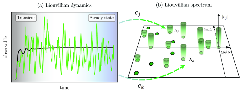
Figure 1: Sketch of steady-state quantum chaos and of the SSQT criterion. (a) Liouvillian dynamics is divided into a transient dynamics where both the density matrix $\hat{\rho}(t)$ and the stochastic quantum trajectory $\ket{\psi(t)}$ time evolve, and a steady-state dynamics, where $\hat{\rho}(t)$ no longer evolves while $\ket{\psi(t)}$ does. A chaotic or integrable steady-state dynamics relies on the behavior of single quantum trajectories. (b) The statistical analysis on the $2D$ Liovillian spectrum identifies an open quantum system as integrable or chaotic. To classify steady-state dynamics as integrable or chaotic, the spectral weights $c_{j}(t)$ defined in Eq. (12) determine the relevance of Liouvillian eigenvalues, and are illustratively represented on the vertical axis. Only some of the Liouvillian eigenvalues have a sizeable weight $|c_{j}|$ and are relevant in determining the steady-state dynamics. On this selected set of Liouvillian eigenvalues, universal predictions of non-Hermitian random matrix theory distinguish regular and chaotic steady-state motion.

II Motivation and overview of the results

II.1 The quantum chaos conjecture

Before illustrating the original results, we review the basic concepts of quantum chaos.

The statistical distribution of the spacings between neighboring Hamiltonian eigenvalues is conjectured to be a universal signature of quantum chaos in closed – i.e., isolated – quantum systems, as first described in Ref. [78] and verified in many instances (see Refs. [54, 55] and references therein). In chaotic systems, energy levels are characterized by level repulsion, absent in integrable systems due to the presence of conserved quantities. In particular, Berry and Tabor conjectured that an Hermitian system characterized by an integrable dynamics in the classical limit, exhibits a spectrum whose spacings are distributed according to the Poissonian statistics typical of uncorrelated random variables [79]. Bohigas, Giannoni, and Schmit (BGS) further theorized that, in a quantum system whose classical limit exhibits chaotic behaviour, the energy level statistics follows the universal spacing distributions of random matrix theory [80, 81]. These properties depend solely on the invariance of the Hamiltonian under time-reversal symmetry [82]. This theoretical framework is known as quantum chaos conjecture. For systems with a well defined classical limit, it has been demonstrated using as argument an unstable periodic orbit pairing mechanism [83, 84, 85, 86, 87]. For systems without a meaningful classical limit (such chains of $1/2$ spins), a rigorous justification of the quantum chaos conjecture has been recently proposed [88].

The quantum chaos conjecture can be generalized to open Markovian systems governed by a (Gorini-Kossakowski-Sudarshan)-Lindblad master equation [56, 89]

$$\begin{split}\frac{\partial\hat{\rho}}{\partial t}&=-i[\hat{H},\hat{\rho}]+\sum_{\mu}\gamma_{\mu}\mathcal{D}[\hat{L}_{\mu}]\hat{\rho},\end{split}$$ (1)

where $\hat{\rho}$ is the reduced density matrix of the system, obtained by tracing out the degrees of freedom of the environment. The Hamiltonian $\hat{H}$ describes the unitary evolution of the system, while the Lindblad dissipator $\mathcal{D}[\hat{L}_{\mu}]$, defined as

$$\mathcal{D}[\hat{L}_{\mu}]\hat{\rho}=\hat{L}_{\mu}\hat{\rho}\hat{L}_{\mu}^{\dagger}-\frac{\hat{L}_{\mu}^{\dagger}\hat{L}_{\mu}\hat{\rho}+\hat{\rho}\hat{L}_{\mu}^{\dagger}\hat{L}_{\mu}}{2},$$ (2)

describes the non-unitary action of the jump operator $\hat{L}_{\mu}$ at a rate $\gamma_{\mu}$. Equation (1) can be recast in the compact form $\partial\hat{\rho}/\partial t=\mathcal{L}\hat{\rho}$ where $\mathcal{L}$ is the (generally non-Hermitian) Liouvillian superoperator.

In this framework, DQC can be characterized via the statistical distribution of the spacings of the complex eigenvalues $\{\lambda_{j}\}$ of the Liouvillian, as first discussed by Grobe, Haake, and Sommers (GHS) [57]. We focus on the distribution of nearest-neighbor eigenvalue spacings

$$p(s)=\sum_{j}\delta(s_{j}-s),$$ (3)

where $s_{j}=|\lambda_{j}-\lambda_{j}^{\rm NN}|$, with $\lambda_{j}^{\rm NN}$ the eigenvalue closest to $\lambda_{j}$ in the complex plane. In analogy to the Hamiltonian case (see Appendix A), $p(s)$ allows distinguishing between chaotic and integrable dynamics. Specifically, in integrable systems $s$ follows a 2D Poisson distribution

$$p_{2D}(s)=\frac{\pi}{2}se^{-\frac{\pi}{4}s^{2}},$$ (4)

while for chaotic systems the spacing follows the Ginibre distribution of Gaussian non-Hermitian random matrices ensembles

$$p_{\textrm{GinUE}}(s)=\left(\prod_{k=1}^{+\infty}\frac{\Gamma(1+k,s^{2})}{k!}\right)\sum_{j=1}^{+\infty}\frac{2s^{2j+1}e^{-s^{2}}}{\Gamma(1+j,s^{2})}.$$ (5)

Finally, the crossover from integrability to chaos in open quantum system is captured by a distribution intermediate between the two [36]. We remark that an unfolding procedure, in which the uncorrelated part is removed from $p(s)$ in Eq. (3), is required to evaluate the level statistics from the spectrum and for the proper characterization of chaos [90]. Throughout this work, we adopt the unfolding procedure detailed in Ref. [36] and reviewed in Appendix A.2. Furthermore, as noticed in Ref. [36], more reliable indicators of chaos and integrability can be obtained by considering the bulk statistics, i.e., the spacing statistics once the eigenvalues close to the real axis have been removed. Here, we will adopt this practice.

A recently introduced quantity that does not require the unfolding procedure, is the complex spacing ratio [40]

$$z_{j}=\frac{\lambda_{j}^{\rm NN}-\lambda_{j}}{\lambda_{j}^{\rm NNN}-\lambda_{j}}=r_{j}e^{i\theta_{j}},$$ (6)

where $\lambda_{j}^{\rm NNN}$ is the second-nearest neighbor to $\lambda_{j}$ in the complex plane. The average values $\langle r\rangle_{L}$ of $r_{j}$ and $\langle\cos(\theta)\rangle_{L}$ of $\cos(\theta_{j})$, can be used as indicators of chaos in the Liouvillian case. For a 2D Poisson distribution $\langle r\rangle_{L}=0.66$, and $-\langle\cos(\theta)\rangle_{L}=0$. For the Ginibre distribution $\langle r\rangle_{L}=0.74$, and $-\langle\cos(\theta)\rangle_{L}=0.24$.

We remark that the Liouvillian eigenvalue statistics describes dissipative chaos as a transient phenomenon and cannot provide a definition of chaos in the steady state, which is associated with a single null eigenvalue [1]. Along the transient, the nature of the dynamics generally depends on the initial state. In this case, the portion of the explored spectrum may be integrable or chaotic depending on the initial conditions. The same dependence on the initial state occurs in closed, Hamiltonian systems. Within the quantum chaos conjecture, therefore, chaos as a property of the quantum dynamics still depends on the choice of the initial conditions.

II.2 Steady-state and transient quantum chaos

An open quantum system converges towards its often unique steady state $\hat{\rho}_{\rm ss}$. Once it has been reached, any memory of the initial condition is lost, and the steady-state properties are only determined by the structure of the Lindblad master equation (1). When studying random Liouvillian systems [42, 41, 49], insight into the chaotic properties of the steady state has been obtained through the study of the entanglement spectrum, that is, the spectrum of the effective Hamiltonian $\hat{H}_{\rm ss}=-\log(\hat{\rho}_{\rm ss})$. As shown in Appendix B, however, the structure of $\hat{\rho}_{\rm ss}$ alone does not provide enough information about chaos or integrability in the general case.

To define and probe chaotic or integrable motion in the steady state, we introduce a criterion that we dub the spectral statistics of quantum trajectories (SSQT). In the steady-state limit, the density matrix is stationary. The density operator is however the average over the statistical ensemble of stochastic quantum trajectories [1, 91, 92, 93], which represent single instances of the system’s dynamics subject to the continuous measurement of the environment [59, 60]. Even in the steady state, quantum trajectories are non-stationary. We argue that it is the dynamics of each individual trajectory that may be chaotic in the steady-state limit. SSQT consists of singling out the set of Liouvillian eigenvalues involved in the dynamics of many independent quantum trajectories (see Fig. 1). This set of eigenvalues determines, according to the quantum chaos conjecture, if the steady state of the system is integrable or chaotic and thus the SSQT criterion relies solely on the spectral structure of the Liouvillian superoperator. As the predictions are drawn from random matrix theory and are applied to the steady state, the SSQT criterion can identify the chaotic or integrable nature of the system independently of the initial condition.

The SSQT criterion can be applied not only to the steady state but also to any arbitrary initial state. In the latter case, however, chaos or integrability will be additionally determined by the initial conditions of the quantum trajectories. The SSQT therefore provides a natural distinction between what we identify as steady-state chaos and transient chaos. The SSQT criterion thus supersedes other spectral criteria and, upon an appropriate choice of initial state, its transient chaos definition recovers the spectral criterion established by the GHS conjecture [57].

We discuss the technical details of the SSQT in the next section. In the appendix B, instead, we provide solid evidence of the generality and reliability of this criterion. In particular, we demonstrate the necessity for its introduction by comparing it to other approaches and demonstrating that models whose Liouvillian spectrum is chaotic according to the spectral criteria can evolve towards either a chaotic or an integrable steady state.

II.3 Chaos in bosonic systems

An important feature of the SSQT criterion is that it allows to study of chaos in bosonic non-particle-number conserving systems. In this work, we investigate the emergence of steady-state and transient quantum chaos in a model which is of great interest both for quantum simulation [20, 94, 95] and quantum computation [73, 8, 9, 10, 11, 76, 21, 22], the driven-dissipative Bose-Hubbard model.

Let us briefly clarify the challenge in discussing chaos in these systems. More details on challenges related to the absence of $U(1)$ symmetry are discussed in appendix C. Quantum chaos in number-conserving (i.e., $U(1)$-symmetric) bosonic systems has been extensively studied both in the classical and quantum regime [96, 97, 98, 99, 100, 101, 102, 103, 104, 105, 106, 107]. So far, however, no theoretical characterization of quantum chaos, in the context of the quantum chaos conjecture, in a driven-dissipative system where the $U(1)$ symmetry is lifted has yet been provided. What makes the study of driven systems in the absence of $U(1)$-symmetry challenging, and sets these models apart from other driven or tilted cases, is that now a cutoff in the otherwise infinite-dimensional bosonic Hilbert space has to be provided. Failing to do that results in spectral statistics that are dominated by states with large particle numbers, which are asymptotically integrable thereby hiding possible chaotic dynamics. For isolated systems one can perform the level statistics on a given energy window, corresponding to, e.g., the energy provided by a quench. A similar choice would be arbitrary for the $2D$ Liouvillian spectrum, as concepts such as energy break down in a Liouvillian framework. Furthermore, from a mathematical point of view, it makes little sense to order the Liouvillian eigenvalues, as they are complex. The SSQT criterion, instead, automatically determines the relevant eigenvalues along the driven-dissipative dynamics that need to be analyzed.

The application of the SSQT to a driven-dissipative Bose-Hubbard model shows that steady-state chaos characterizes a large portion of parameter space, as we show through the numerical analysis of a one-photon driven-dissipative Bose-Hubbard dimer. Interestingly, the parameter region where we observe transient chaos is larger than the one characterized by steady-state chaos. The phase diagram becomes even richer when we explore the classical (or mean-field) and semi-classical (taking into account quantum correlations at lowest orders in $\hbar$) limits of the model. Here, two different types of steady-state DQC emerge. The first one, characterized by super-Poissonian fluctuations, partially captured by the mean-field analysis and completely by the semi-classical approach, obeys the GHS conjecture for the quantum-to-classical correspondence. The second one, displaying sub-Poissonian fluctuations, has neither a classical nor a semi-classical limit, thus transcending the GHS conjecture. This latter steady-state DQC constitutes therefore an emergent feature of driven-dissipative bosonic quantum systems.

III Spectral statistics of quantum trajectories

In this section, we define the theoretical framework for the characterization of steady-state and transient quantum chaos in open quantum systems.

The Lindblad master equation (1) with jump operators (2) can be recast in the form $\partial\hat{\rho}/\partial t=\mathcal{L}\hat{\rho}$ where the Liouvillian $\mathcal{L}$ is the non-Hermitian generator of dissipative dynamics. As $\hat{\rho}(t)=\exp(\mathcal{L}t)\hat{\rho}(0)$, the eigendecomposition of $\mathcal{L}$ fully characterizes the dynamics of the density matrix. The right eigenoperators $\hat{\eta}_{j}$ and left eigenoperators $\hat{\sigma}_{j}$ of $\mathcal{L}$ [1] are defined by

$$\mathcal{L}\hat{\eta}_{j}=\lambda_{j}\hat{\eta}_{j},\,\,\,\,\,\,\,\,\,\mathcal{L}^{\dagger}\hat{\sigma}_{j}=\lambda_{j}^{*}\hat{\sigma}_{j},$$ (7)

and satisfy the biorthonormality condition $\operatorname{Tr}\{\hat{\sigma}_{j}^{\dagger}\hat{\eta}_{l}\}=\delta_{jl}$. The most general density matrix $\hat{\rho}(t)$ can thus be decomposed as [108]

$$\hat{\rho}(t)=\sum_{j}c_{j}(t)\,\hat{\eta}_{j},$$ (8)

with spectral weights $c_{j}(t)=\operatorname{Tr}\{\hat{\sigma}_{j}^{\dagger}\hat{\rho}(t)\}$.

The steady state $\hat{\rho}_{\rm ss}$ is defined as the state which does not evolve under the action of the Liouvillian, $\mathcal{L}\hat{\rho}_{\rm ss}=0$. As such, $\hat{\rho}_{\rm ss}$ is the right eigenoperator of the Liouvillian associated with the eigenvalue $\lambda_{0}=0$. For the models we consider in this paper, the steady state is unique and $\hat{\rho}_{\rm ss}=\lim_{t\to\infty}\hat{\rho}(t)$.

The master equation (1) admits also a stochastic unraveling in terms of quantum trajectories $\ket{\psi(t)}$, combining the Hamiltonian dynamics with a continuous monitoring of the environment [59, 60]. For a counting trajectory , within each time step $dt$ a quantum jump occurs with probability $dp=\gamma\sum_{\mu}\bra{\psi(t)}\hat{L}_{\mu}^{\dagger}\hat{L}_{\mu}\ket{\psi(t)}dt$ and $\ket{\psi(t)}$ evolves into

$$\ket{\psi(t+dt)}\propto\hat{L}_{\mu}\ket{\psi(t)},$$ (9)

where the jump operator $\hat{L}_{\mu}$ is sampled from the probability distribution

$$p_{\mu}=\frac{\bra{\psi(t)}\hat{L}_{\mu}^{\dagger}\hat{L}_{\mu}\ket{\psi(t)}}{\sum_{\mu}\bra{\psi(t)}\hat{L}_{\mu}^{\dagger}\hat{L}_{\mu}\ket{\psi(t)}}.$$ (10)

With probability $1-dp$ no quantum jump occurs, and $\ket{\psi(t)}$ evolves into

$$\ket{\psi(t+dt)}\propto(\mathds{1}-idt\hat{H}_{\rm nh})\ket{\psi(t)},$$ (11)

where $\hat{H}_{\rm nh}=\hat{H}-i\sum_{\mu}\gamma_{\mu}\hat{L}_{\mu}^{\dagger}\hat{L}_{\mu}/2$ is the non-Hermitian Hamiltonian. After each time step, the state $\ket{\psi(t+dt)}$ is renormalized.

Consider a quantum system, characterized by quantum trajectories $\ket{\psi_{m}(t)}$, where $m$ labels each independent quantum trajectory evolving according to Eqs. (9) and (11). Using the spectral decomposition introduced in Eq. (8), one can define

$$\begin{split}\hat{\rho}_{m}(t)=&\outerproduct{\psi_{m}(t)}{\psi_{m}(t)}=\sum_{j}c_{m,j}(t)\,\,\hat{\eta}_{j}.\end{split}$$ (12)

This procedure allows associating to each eigenvalue $\lambda_{j}$ the relative spectral weight $c_{m,j}(t)$. We initialize the system in a given initial state $\ket{\psi_{m}(0)}=\ket{\psi_{0}}\,\forall m$. We then let the trajectories evolve for a time $t$ and compute their spectral decomposition according to Eq. (12). We then construct the set of $(\lambda_{j},\vec{c}_{j})_{m}$, corresponding to each trajectory. DQC is usually characterized through the statistical properties of $\{\lambda_{j}\}$ [57, 36, 40]. Here, we argue instead that DQC is encapsulated in both $\lambda_{j}$ and $\vec{c}_{j}$.

We name the above procedure spectral statistics of quantum trajectories (SSQT). The SSQT criterion is illustrated in Fig. 1. While the steady-state density matrix does not evolve in time (and thus expectation values are stationary), steady-state dynamics of single quantum trajectories displays integrable or chaotic behaviour [Fig. 1(a)]. To determine the presence of DQC from $(\lambda_{j},\vec{c}_{j})_{m}$, we propose to select the Liouvillian eigenvalues $\lambda_{j}$, for which the trajectory $\ket{\psi_{m}(t)}$ has a sizeable spectral component, i.e. $|c_{m,j}(t)|>c_{\rm min}$ [Fig. 1(b)]. The cutoff $c_{\rm min}$ selects the eigenvalues and eigenoperators that are physically relevant at time $t$. Only on these we perform the analysis of the statistical distribution of the Liouvillian eigenvalue distances. Results are finally averaged on a given number of independent quantum trajectories . We denote the number of the relevant eigenvalues at time $t$ with $N_{\lambda}(t)$.

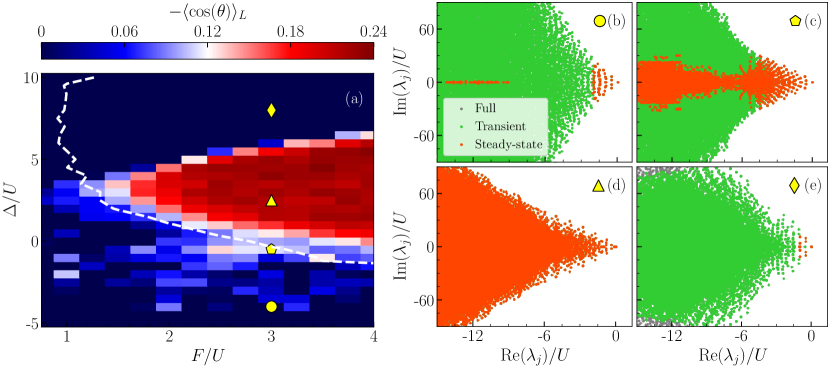
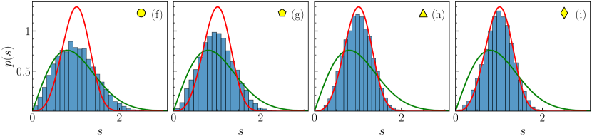
Figure 2: Steady-state and transient dissipative quantum chaos in the Bose-Hubbard dimer using the SSQT criterion described in Sec. III. (a) Phase diagram of the single number indicator $-\langle\cos(\theta)\rangle_{L}$ as a function of the detuning $\Delta/U$ and of the drive $F/U$. The colormap refers to steady-state chaos (results are obtained upon averaging over $100$ independent quantum trajectories), while the dashed white line bounds the region of transient chaos. (b-e) Liouvillian spectra for $F/U=3$, and increasing values of $\Delta$. The full spectrum is denoted by gray dots. The relevant eigenvalues for the transient (green dots) and the steady-state (red dots) cases are superimposed. All data have been obtained by numerically diagonalizing the Liouvillian, and selecting the relevant eigenvalues with $c_{\rm min}=10^{-5}$ (see Appendix A.3). The initial state is the coherent state $\ket{\psi_{m}(0)}=\ket{\alpha}\otimes\ket{\alpha}$ for $\alpha=3\sqrt{F/(\Delta-i\gamma)}$. When the number of selected eigenvalues is $N_{\lambda}<100$, a statistically significant analysis cannot be carried out, and we set $-\langle\cos(\theta)\rangle_{L}=0$. The values of the detuning are: (b) $\Delta/U=-4$, (c) $\Delta/U=-0.5$, (d) $\Delta/U=2.5$, (e) and $\Delta/U=8$. Other parameters are set to $J/U=2$ and $\gamma/U=1$. The cavity cutoff has been fixed to $N_{c}=13$. (f-i) Histograms of the spacing distribution $p(s)$ calculated over the relevant spectrum selected according to the SSQT criterion applied at $t=0$ over the same four points selected in panels (b-e). The green (red) curve is a guideline indicating an ideal 2D-Poisson (Ginibre) distribution.

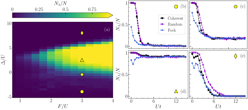
Figure 3: Analysis of the number of relevant eigenvalues $N_{\lambda}(t)$ obtained with the SSQT criterion in Sec. III for the Bose-Hubbard dimer. (a) $N_{\lambda}$ at the steady state as a function of the detuning $\Delta/U$ and of the drive $F/U$. The initial state is the coherent state chosen for Fig. 2(a). The phase diagram is obtained upon averaging over $100$ independent quantum trajectories. (b-e) As a function of time, $N_{\lambda}(t)$ for $F/U=3$, and increasing values of $\Delta$ as in Fig. 2(b-e) for three different types of initial states: the coherent states chosen for Fig. 2(b-e), Fock states $\ket{\psi_{m}(0)}=\ket{n}\otimes\ket{n}$ with $n$ randomly chosen between $[0,5]$ for each trajectory, and random vectors $\ket{\psi_{m}(0)}$ in the Hilbert space. While transient dynamics exhibits different values of $N_{\lambda}$, depending on the type of initial state $\ket{\psi_{m}(0)}$, the steady-state dynamics does not depend on this choice. Data are computed upon averaging over $30$ independent quantum trajectories.

The choice of the time $t$, at which the analysis is carried out, is key to the distinction between transient and steady-state quantum chaos. If $t$ is chosen within the early stages of the dynamics, our criterion characterizes transient chaos. In this case, the chaotic or integrable nature of the system will in general depend on the initial condition $\hat{\rho}(0)$. If instead $t$ is chosen so that $\hat{\rho}(t)\simeq\hat{\rho}_{\rm ss}$ then the analysis will single out the steady-state properties, defining a criterion for steady-state chaos.

The choice of $c_{\rm min}$ needs to be physically justified, and may be model-dependent (see, e.g., the discussion in Appendix A.3 for the models considered below), however, the predictions we draw from $(\lambda_{j},\vec{c}_{j})$ remain universal. Incidentally, this approach also solves the issue of selecting the relevant subspace of eigenvalues when studying infinite-dimensional bosonic systems, as discussed in Appendix C.

We remark that when the system is invariant under weak or strong symmetries [111, 112], the portion of the Hilbert space spanned by a quantum trajectory may depend on the specific unraveling [113, 114]. For models that are not invariant under any symmetry, such as the ones considered below, we expect (and numerically verify) that the specifics of the unraveling play a negligible role.

IV Steady-state and transient chaos in driven-dissipative bosonic systems

We study now the emergence and the features of steady-state and transient DQC in a one-dimensional boundary-driven and boundary-dissipative Bose-Hubbard dimer, made of two coupled driven-dissipative nonlinear resonators. In the frame rotating at the frequency of the driving (pump) field, the Hamiltonian of the system reads

$$\begin{split}\hat{H}&=\sum_{j=1}^{2}\left(-\Delta\hat{a}_{j}^{\dagger}\hat{a}_{j}+\frac{1}{2}U\hat{a}_{j}^{\dagger}\hat{a}_{j}^{\dagger}\hat{a}_{j}\hat{a}_{j}\right)\\ &-J\left(\hat{a}_{2}^{\dagger}\hat{a}_{1}+\hat{a}_{1}^{\dagger}\hat{a}_{2}\right)+F(\hat{a}_{1}^{\dagger}+\hat{a}_{1}),\end{split}$$ (13)

where $\hat{a}_{j}^{\dagger}$ and $\hat{a}_{j}$ are the bosonic creation and annihilation operators of the $j$-th cavity mode. Here, $\Delta=\omega_{p}-\omega_{c}$ is the pump-to-cavity detuning, $U$ is the strength of the Kerr nonlinearity, $J$ is the hopping strength, and $F$ is the driving field amplitude. Losses are assumed to act analogously on both cavities with photon loss being the dominant dissipation process. The dynamics of the system is described by the master equation

$$\frac{\partial\hat{\rho}}{\partial t}=-i[\hat{H},\hat{\rho}]+\gamma\sum_{j=1}^{2}\left(\hat{a}_{j}\hat{\rho}\hat{a}_{j}^{\dagger}-\frac{1}{2}\anticommutator{\hat{a}_{j}^{\dagger}\hat{a}_{j}}{\hat{\rho}}\right),$$ (14)

where $\gamma$ is the loss rate, and $\hat{H}$ is given by Eq. (13). As discussed above, the master equation (14) admits a stochastic unravelling in terms of quantum trajectories. As the model we consider is not invariant under any weak or strong Liouvillian symmetry [112, 111], we expect the results to be independent of the unraveling [113, 114]. Without loss of generality, throughout the paper, we employ a photon-counting unraveling because of its numerical efficiency.

As detailed in Appendix C, in the presence of a driving field, the $U(1)$ invariance of the bare model is lifted, particle number is no longer conserved, and states evolve in time to potentially cover the entirety of the Hilbert space. In Hubbard-like models, the local interaction term scales as $U\langle\hat{a}^{\dagger\,2}\hat{a}^{2}\rangle\sim Un^{2}$ with the remaining terms scaling at most linearly in the cavity occupation $n=\langle\hat{a}^{\dagger}\hat{a}\rangle$. It follows that the infinitely many large-occupancy eigenstates are decoupled, and behave as single anharmonic oscillators. Their spectral contribution dominates over that of all other states, resulting in an integrable level statistics, independently of the statistics of the spectrum at lower occupancy. The SSQT criterion provides a natural way to select the relevant portion of the spectrum, ensuring that the selected eigenvalues do not incur in this asymptotic decoupling issue.

IV.1 The driven-dissipative Bose-Hubbard dimer

In what follows we report numerical results on the application of the SSQT criterion to the Bose-Hubbard dimer. All calculations have been performed on the Quantum Optics Toolbox in Python (QuTiP) [115, 116].

Figure 2(a) shows the indicator $-\langle\cos(\theta)\rangle_{L}$, computed as a function of $\Delta/U$ and $F/U$, for the eigenvalues relevant to the steady-state . The result clearly identifies a steady-state chaotic phase emerging for sufficiently large values of $F$ and an appropriate choice of $\Delta$. The dashed line in Fig. 2(a) highlights the phase boundary between the integrable and chaotic regions, as obtained by applying the criterion for transient chaos at $t=0$. As initial state we choose the coherent state $\ket{\psi_{m}(0)}=\ket{\alpha}\otimes\ket{\alpha}$ for $\alpha=3\sqrt{F/(\Delta-i\gamma)}$. The choice is justified as in experimental settings an initial coherent state can be easily prepared. The phase boundary coincides with that of steady-state chaos in the region of negative detuning. For large positive values of $\Delta$ instead, the diagram shows a region where transient chaos occurs in spite of an integrable steady state. Liouvillian spectra with the relevant eigenvalues, for the points highlighted in Fig. 2(a), are displayed in Figs. 2(b-e). The spacing distributions (3) associated to each of these points, for the transient dynamics, are plotted in Figs. 2(f-i). We observe that while our criterion clearly classifies the latter steady-state dynamics [Fig. 2(e)] as completely regular (only a few eigenvalues are involved in the dynamics), a spectral analysis on many Liouvillian eigenvalues [Fig. 2(i)] does not allow to draw any conclusion on the nature of the steady state.

We now relax the requirement that we start from a coherent state and we consider three different types of initial states: coherent states, Fock states, and random vectors in the Hilbert space. The analysis of the number of relevant eigenvalues $N_{\lambda}(t)$ is shown in Fig. 3. In the steady state, we note a direct correspondence between the $\langle\cos(\theta)\rangle_{L}$ and $N_{\lambda}$ [c.f Figs. 2(a) and 3(a)]. In the transient dynamics, instead, we find that $\langle\cos(\theta)\rangle_{L}(t)\simeq\langle\cos(\theta)\rangle_{L}(0)\,N_{\lambda}(t)/N_{\lambda}(0)$. We plot $N_{\lambda}(t)$ in Fig. 3(b-e). As expected, transient dynamics depend on the type of initial states, while the steady-state dynamics does not depend on this choice. We remark that this feature is in stark contrast with the unitary dynamics of an isolated quantum system, where the selected eigenvalues depend solely on the initial state (once a cutoff value $c_{\rm min}$ has been set). Indeed the spectral weights $c_{j}(t)$ in Eq. (8) reduce to $|c_{j}(t)|=|\bra{\phi_{j}}\ket{\psi(t)}|=|e^{-iE_{j}t}\bra{\phi_{j}}\ket{\psi(0)}|=|\bra{\phi_{j}}\ket{\psi(0)}|$ where $E_{j},\ket{\phi_{j}}$ are the eigenvalues and eigenvectors of the Hamiltonian and $\ket{\psi(t)}$ solves the Schrödinger equation.

IV.2 Classical vs Liouvillian analysis

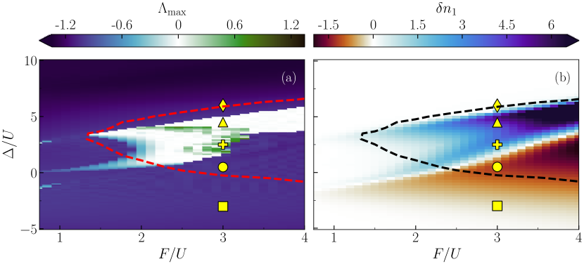
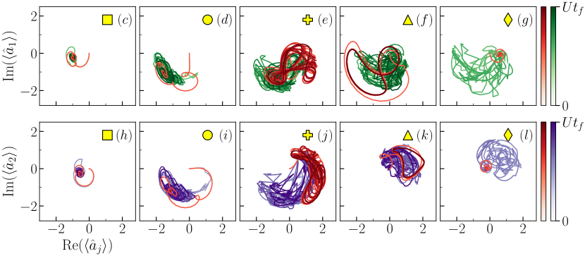
Figure 4: Classical vs full quantum analysis. (a) The largest Lyapunov exponent $\Lambda_{\rm max}$, calculated according to the method in Appendix A.4. The system displays a stripe of limit cycles $\Lambda_{\rm max}=0$, and within this region we find classical chaos $\Lambda_{\rm max}>0$. The dashed red line bounds the region of steady-state quantum chaos. (b) Deviation from Poissonian distribution $\delta n_{1}$, defined in Eq. (16), for the first cavity. The region with super-Poissonian light ($\delta n_{1}>0$) coincides with the classical region hosting limit cycles and strange attractors. The steady-state quantum chaotic region (dashed line) extends over both the super-Poissonian and sub-Poissonian regions. (c-g) Single classical (in red) and quantum trajectory (in green) with $Ut_{f}=30$ for the first cavity, (h-l) the same but for the second cavity (quantum trajectories are in purple). The five cases correspond to selected parameter values highlighted with different symbols in panel (a). (c) and (h) Both the classical and the quantum solutions approach a fixed point. (d) and (i) The classical case approaches a fixed point, while the quantum trajectory displays a chaotic attractor. (e) and (j) Both the classical and quantum trajectories show chaotic attractors. (f) and (k) The classical trajectory displays a limit cycle while the quantum trajectory shows a chaotic attractor. (g) and (l) the classical trajectory approaches a fixed point, while the quantum trajectory displays transient chaotic behaviour before approaching the fixed point. The values of detunings are: (c) and (h) $\Delta/U=-3$, (d) and (i) $\Delta/U=0.5$, (e) and (j) $\Delta/U=2.5$, (f) and (k) $\Delta/U=4.5$, (g) and (l) $\Delta/U=6$. $F/U$, $J/U$ and $\gamma/U$ set as in Fig. 2.

The study of the classical limit offers a unique viewpoint to understand the origin of dissipative quantum chaos. To study it, we employ the Gross-Pitaevskij mean-field approximation . For each resonator in the Bose-Hubbard chain, we assume that $\hat{\rho}=\bigotimes_{j}\hat{\rho}_{j}$ at all times, with $\hat{\rho}_{j}=\outerproduct{\alpha_{j}}{\alpha_{j}}$ and $\hat{a}_{j}\ket{\alpha_{j}}=\alpha_{j}\ket{\alpha_{j}}$ [119, 120, 121]. Doing so for the master equation (14) leads to

$$\frac{\partial}{\partial t}\alpha_{1} =\left(i\Delta-\frac{1}{2}\gamma\right)\alpha_{1}-iU|\alpha_{1}|^{2}\alpha_{1}+iJ\alpha_{2}-iF\,,$$ (15)

$$\frac{\partial}{\partial t}\alpha_{2} =\left(i\Delta-\frac{1}{2}\gamma\right)\alpha_{2}-iU|\alpha_{2}|^{2}\alpha_{2}+iJ\alpha_{1}\,.$$

Classical chaos for dynamical systems is mainly characterized through the Lyapunov exponents $\Lambda$ [122]. The system is chaotic if the largest Lyapunov exponent $\Lambda_{\rm max}$ is strictly positive. Lyapunov exponents can also distinguish bounded attractors hosting limit cycles from dense regions in phase space where classical chaos arises. We evaluate $\Lambda_{\rm max}$ as a function of $\Delta/U$ and $F/U$. Details on the numerical estimation of the largest Lyapunov exponent are reported in the Appendix A. The results are shown in Fig. 4 (a). We observe a large region characterized by a vanishing Lyapunov exponent, where the system dynamics follows a limit cycle. Within this region, a smaller chaotic region is present, where the dynamics are characterized by a strange attractor with a positive Lyapunov exponent. The behavior of selected classical phase-space trajectories is displayed in Fig. 4(c-l), showing fixed-point, limit-cycle, and chaotic behavior depending on the selected values of the model parameters. The comparison of the classical phase diagram with that for steady-state dissipative quantum chaos clearly shows that the quantum system displays chaos in a larger region of the parameter space than its classical limit. This finding supports existing evidence [44] that for driven-dissipative systems, the correspondence between quantum chaos and chaotic behavior in the classical limit [57] does not hold in general.

To gain more insight into the emergence of dissipative quantum chaos for parameters where the classical limit is not chaotic, we inspect the properties of single quantum trajectories and study the fluctuations in the photon number. We define the deviation from the Poissonian distribution

$$\delta n_{j} =\langle\hat{a}_{j}^{\dagger}\hat{a}_{j}^{\dagger}\hat{a}_{j}\hat{a}_{j}\rangle_{\rm ss}-\langle\hat{a}_{j}^{\dagger}\hat{a}_{j}\rangle_{\rm ss}^{2}$$ (16)

$$=(\Delta{n}_{j})^{2}-\langle\hat{n}_{j}\rangle_{\rm ss}$$

where $\langle\hat{O}\rangle_{\rm ss}\equiv\operatorname{Tr}\{\hat{\rho}_{\rm ss}\hat{O}\}$ and $(\Delta{n}_{j})^{2}=\langle\hat{n}_{j}^{2}\rangle_{\rm ss}-\langle\hat{n}_{j}\rangle_{\rm ss}^{2}$. The quantity in Eq. (16) is zero for Poissonian photon-number statistics, and takes positive (negative) values for a super (sub)-Poissonian distribution. The quantity $\delta n_{1}$ is plotted in Fig. 4(b). From the data, it clearly appears that the parameters for which steady-state chaos occurs define two distinct regions in parameter space, characterized by different photon-number statistics. In one region, the system displays super-Poissonian statistics, and comparison with Fig. 4(a) indicates that in the same region the classical limit displays either chaos or limit cycles. The other region is characterized by sub-Poissonian statistics, and the classical limit is correspondingly characterized by fixed points. While Poissonian or super-Poissonian light admits a classical description, sub-Poissonian light arises from genuine quantum mechanical effects [123].

In Figs. 4(c-l), we plot the expectation value of the field in each cavity along a single quantum trajectory, for several points in parameter space. The plots also display the same quantities computed in the classical limit for the same initial condition. Panels (c) and (h) correspond to a steady-state integrable system. In this case, both the classical and quantum trajectories approach fixed points, with the quantum trajectories displaying few quantum jumps along their dynamics. Panels (d) and (i) correspond to steady-state chaos with sub-Poissonian photon-number statistics. Here, the classical trajectory approaches a fixed point, but quantum jumps prevent the quantum trajectory from reaching the same fixed point. Hence, chaos here arises exclusively due to the fluctuations induced by the environment. Each quantum jump resets the quantum trajectory to a random state and prevents the system from reaching the classical fixed point, in a way that is reminiscent of the quantum Zeno effect [124]. The sub-Poissonian statistics is therefore explained, as the variations in the photon number along the dynamics are due to the quantum jumps, which are random events with a sub-Poissonian distribution. Panels (e) and (j) correspond to parameters for which both the classical and quantum systems are chaotic. Here, the classical trajectories display a chaotic attractor, and the quantum trajectories are similarly characterized by a chaotic attractor randomly perturbed by quantum jumps. Panels (f) and (k) correspond to parameters where the classical system displays a limit cycle, which clearly appears for the classical trajectories. Here, the quantum trajectories are characterized by a chaotic attractor, as the trajectory is randomly perturbed by quantum jumps. The super-Poissonian statistics in the two latter cases are inherited from the classical limit. Indeed, along the dynamics of both a chaotic attractor and a limit cycle, the field intensity randomly varies from small to large values along a continuous curve, thereby resulting in super-Poissonian statistics typical of fluctuating classical fields [125]. Dissipative quantum chaos in the two latter cases emerges as additional fluctuations induced by quantum jumps along the dynamics. The fluctuations do not alter the photon-number statistics but, in the case with classical limit cycles, result in fluctuation-induced chaotic dynamics. Finally, panels (g) and (l) display a case where transient chaos but integrable steady-state occur. Here again, the quantum trajectory is characterized by a chaotic behavior solely induced by fluctuations, while the classical trajectory regularly approaches a fixed point.

The overall analysis provides a clear explanation of the nature of steady-state dissipative quantum chaos. In a driven-dissipative system, steady-state chaos can be caused by environment-induced fluctuations which reset the quantum trajectories at random times, effectively preventing the system from following its classical path in phase-space. This picture explains why dissipative quantum chaos occurs on a significantly larger region of parameters than that characterized by classical chaos, where the classical limit only displays fixed points or limit cycles. It provides a justification of why, in driven-dissipative quantum systems, a correspondence similar to the BGS correspondence [81] in Hamiltonian quantum systems does not hold in general.

IV.3 Semi-classical analysis

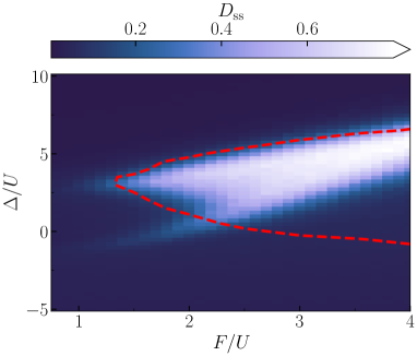
Figure 5: Semi-classical analysis. Semi-classical OTOC for the first cavity $D_{\rm ss}$ computed within the truncated Wigner approximation (TWA) averaging over $1000$ independent Wigner stochastic trajectories. The region displaying semi-classical chaos ($D_{\rm ss}\simeq 1$) matches the quantum region characterized by super-Poissonian fluctuations in Fig. 4(b) and extends only slightly beyond the classical region characterized by $\Lambda_{\textrm{max}}\geq 0$ in Fig. 4(a). The dashed line delimits the region of steady-state quantum chaos. The quantum chaotic region characterized by sub-Poissonian fluctuations is not captured by the quantum corrections provided by TWA. Physical parameters chosen as in Fig. 2(a).

To gain further insight into the nature of DQC, we now include quantum fluctuations in a perturbative way. The question we address is, whether the DQC observed in the full quantum description can be already captured perturbatively, or rather is an intrinsic quantum mechanical feature. Various approaches have been proposed to model quantum dynamics perturbatively in the quantum effects. Among them, cluster mean-field approaches [126, 127], quantum cumulant expansions [128, 129, 130] and the truncated Wigner approximation (TWA) [131, 132, 133] stand out. All these approaches are semi-classical, in the sense that they account for quantum effects only perturbatively. Here, we adopt the TWA, which has proven successful in the characterization of open and closed bosonic systems (see for example Refs. [134, 135, 136]). Within the Wigner formalism, the full Lindblad equation (14) is mapped onto a partial differential equation for the Wigner function. This mapping is exact, but the many-body interactions lead to terms of high order whose numerical treatment is highly challenging. The TWA consists in discarding these high-order terms and keeping only terms of second order. The approximation corresponds to accounting for quantum effects only to leading order in $\hbar$. Then, the equation for the Wigner function reduces to a Fokker-Plank equation which can be mapped onto the set of stochastic differential equations for the phase-space variables.

$$\frac{\partial}{\partial t}\alpha_{1} =\left(i\Delta-\frac{1}{2}\gamma\right)\alpha_{1}-iU(|\alpha_{1}|^{2}-1)\alpha_{1}$$ (17)

$$+iJ\alpha_{2}-iF+\xi(t)\sqrt{\gamma/2}\,,$$

$$\frac{\partial}{\partial t}\alpha_{2} =\left(i\Delta-\frac{1}{2}\gamma\right)\alpha_{2}-iU(|\alpha_{2}|^{2}-1)\alpha_{2}$$

$$+iJ\alpha_{1}+\xi(t)\sqrt{\gamma/2}\,.$$

Here, $\xi$ is a stochastic Wiener process such that $\langle\xi(t)\xi^{*}(t^{\prime})\rangle=\delta(t-t^{\prime})$.

To study quantum chaos within the TWA, we employ the semi-classical out-of-time-order correlator (OTOC) introduced in [137] for spin systems and successfully applied to many-body classical and semi-classical systems [138, 139, 140, 141, 142, 143]. In the present case, the semi-classical OTOC can be defined as

$$D(t)=1-\frac{\langle\alpha^{*}_{a}(x,t)\alpha_{b}(x,t)\rangle}{\langle\alpha^{*}_{a}(x,t)\alpha_{a}(x,t)\rangle},$$ (18)

where $\alpha_{a,b}$ are copies of the systems differing by $|\varepsilon|\ll 1$ in the initial condition. We denote with $\langle\cdot\rangle$ the proper statistical average. As detailed in [137], $D(t)$ measures how replicas of the system correlate in time. For an integrable system, the two replicas are expected to remain correlated over a long time, so that $D(t)=0$. For a fully chaotic system on the other hand, the two replicas will rapidly lose correlation, leading to $D(t)=1$. Here we consider two solutions $\alpha_{a}(t)$ and $\alpha_{b}(t)$ of Eqs. (17), obtained from the same noise realization, but such that $\alpha_{b}(0)=\alpha_{a}(0)+\varepsilon$, where we take $\varepsilon=0.01(1+i)/\sqrt{2}$. As we are interested in the steady-state limit, we let the system evolve for sufficiently long times, until observables become stationary. We then compute the $L^{2}$ distance (the specific choice of the metric is not relevant) between the solutions $\alpha$ and $\tilde{\alpha}$, defined as

$$\begin{split}d_{L^{2}}(\alpha,\tilde{\alpha})&=\sqrt{[\textrm{Re}(\tilde{\alpha})-\textrm{Re}(\alpha)]^{2}+[\textrm{Im}(\tilde{\alpha})-\textrm{Im}(\alpha)]^{2}}.\end{split}$$ (19)

When the Bose-Hubbard dimer is integrable, $d_{L^{2}}$ is equal to zero, while for chaotic dynamics, $d_{L^{2}}$ takes large positive values. We then define the steady-state semi-classical OTOC

$$D_{\rm ss}=1-\left\langle e^{-d_{L^{2}}(\alpha,\tilde{\alpha})}\right\rangle$$ (20)

where $\langle\cdot\rangle$ is the statistical average over many independent Wigner trajectories. $D_{\rm ss}$ is zero for integrable systems and one for fully chaotic systems.

Results are reported in Fig. 5 for the first cavity. The quantity $D_{\rm ss}$ is computed by averaging over $1000$ independent Wigner trajectories. The region characterized by $D_{\rm ss}\simeq 1$ matches the quantum chaotic region characterized by super-Poissonian fluctuations and extends slightly beyond the classical region exhibiting $\Lambda_{\rm max}\geq 0$. However, similarly to the mean-field analysis, also the semi-classical approach fails to predict chaos in the quantum chaotic region characterized by sub-Poissonian fluctuations.

This finding provides final evidence to the fact that this kind of steady-state quantum chaos is an emergent feature of driven-dissipative bosonic systems, lacking any classical or semi-classical counterparts. It demonstrates the unique nature of DQC, and highlights its fundamental difference from quantum chaos in Hamiltonian systems.

V Conclusions and outlook

We develop a general understanding of chaos and integrability in the dynamics of open quantum systems. In the long-time limit, we show that steady-state quantum chaos or integrability are uniquely encapsulated in the spectral structure of the Liouvillian superoperator. This is in stark contrast with the traditional approach to quantum chaos [54, 55, 36, 40], where the system’s dynamics can be predicted only in a statistical sense, while single examples of dynamics can be either integrable or chaotic depending on the initial condition.

To characterize steady-state dynamics, we introduce a model-independent criterion, the spectral statistics of quantum trajectories (SSQT). We demonstrate that SSQT correctly identifies chaos in several dissipative systems, where other criteria provide ambiguous results. As it relies only on the global structure of the Lindblad master equation, we expect the SSQT to be widely used in future studies for probing the dynamics of open quantum systems.

We apply this theoretical framework to the driven-dissipative Bose-Hubbard model, showing a rich phase diagram where integrability, steady-state and transient chaos coexist. This is the first verification of the quantum chaos conjecture in a non-$U(1)$ symmetric bosonic system. Driven-dissipative bosonic systems are extensively used for applications in quantum technologies [73, 8, 9, 10, 11, 76, 21, 22]. Our work paves the way for the investigation of chaos in realistic quantum computing and sensing devices, where detrimental effects of both classical and quantum chaotic dynamics have been very recently predicted [144, 145, 146]. Understanding the effects of dissipative quantum chaos on the performances of quantum information platforms can be a decisive step toward the realization of fault-tolerant quantum computers.

Driven-dissipative bosonic systems designed for quantum computation [22] and sensing [21] often display weak or strong Liouvillian symmetries. An interesting open question concerns the study of dissipative quantum chaos in systems invariant under Liouvillian symmetries, as in this case the results are expected to depend significantly on the specific unraveling of the master equation [113].

The comparison between quantum, semi-classical and mean-field classical limit suggests that different kinds of steady-state chaos can exist. We identify a kind of steady-state quantum chaos that persists in both the classical (where all quantum correlations are neglected) and semi-classical (considering short-range quantum correlations) limits, thus obeying the GHS conjecture [57]. We also characterize an emergent steady-state quantum chaos without any classical or semi-classical limit. The study of individual quantum trajectories and of the boson-number fluctuations in bosonic systems indicates that dissipative quantum chaos may emerge in an otherwise classically integrable system as a result of quantum fluctuations, which cause random deviations from regular phase-space trajectories, effectively turning them into chaotic attractors. Further study is warranted to systematically understand which conditions can lead to the departure from the GHS conjecture in open quantum systems.

Appendix A Details on methods

A.1 Hamiltonian unfolding

The spectrum of a given Hamiltonian must be unfolded in order to characterize the integrable or chaotic statistics. The unfolding procedure allows distinguishing the fluctuations, which are universal, from the averaged spectral density, which is system-specific. For real eigenvalues, the unfolding can be achieved as explained in Ref. [147] by introducing the spectral function and its cumulative function

$$S(E)=\sum_{i=1}^{N}\delta(E-E_{n}),\,\,\,\,\,\eta(E)=\sum_{i=1}^{N}\Theta(E-E_{n}).$$ (21)

The cumulative function decomposes into a smooth part and a fluctuating part

$$\eta(E)=\eta_{av}(E)+\eta_{fl}(E).$$ (22)

The smooth part can be fitted with a polynomial $\tilde{\eta}_{av}(E)$ and the spectrum $\{E_{1},...,E_{N}\}$ is mapped onto the unfolded spectrum $\{\xi_{1},..,\xi_{N}\}=\{\tilde{\eta}_{av}(E_{1}),...,\tilde{\eta}_{av}(E_{N})\}$.

A.2 Liouvillian unfolding

For open systems the eigenvalues $\lambda_{j}$ are complex-valued. Unfolding is similarly achieved by separating the universal fluctuations from the averaged system-specific density

$$\rho(\lambda)=\sum_{j=1}^{N}\delta^{(2)}(\lambda-\lambda_{j})=\rho_{av}(\lambda)+\rho_{fl}(\lambda).$$ (23)

The method proposed by [36] consists in approximating the sum of delta functions with the smooth sum of Gaussians

$$\tilde{\rho}_{av}(\lambda)\simeq\frac{1}{2\pi\sigma^{2}N}\sum_{j=1}^{N}\exp\left(-\frac{1}{2\sigma^{2}}|\lambda-\lambda_{j}|^{2}\right).$$ (24)

Then the $j$-th spacing $s_{j}=|\lambda_{j}-\lambda_{j}^{\rm NN}|$ is mapped onto $s_{j}^{\prime}=s_{j}\sqrt{\tilde{\rho}_{av}(\lambda_{j})}/\bar{s}$, where $\bar{s}$ is chosen such that $\sum_{j=1}^{N}s_{j}^{\prime}/N=1$, and the statistical distribution of $s_{j}^{\prime}$ is evaluated.

The parameter $\sigma$ should be chosen so to make the unfolding procedure effective. It was found [36] that setting $\sigma=4.5\times\sum_{j=1}^{N}s_{j}/N$ achieves such an optimal unfolding.

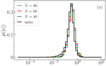
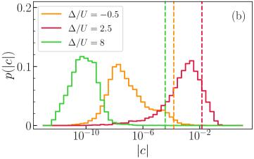
Figure 6: Distribution $p(|c|)$ obtained by binning the weights $\{|c_{m,j}|\,\forall m,j\}$ as described in the text. (a) $p(|c|)$ for the random chaotic Liouvillian described in Sec. B.1 , and different sizes of the Hilbert space. In black, we also superimpose the distribution for the spin model in Sec. B.2 in the deeply chaotic configuration $F/J=1$. (b) $p(|c|)$ for the Bose-Hubbard model described in Sec. IV and different detunings, having fixed $F/U=3$, $J/U=2$ and $\gamma/U=1$.

A.3 Choice of $c_{\rm min}$

Consider a set of quantum trajectories and the corresponding $(\lambda_{j},\vec{c}_{j})$ as defined in Sec. III. The distribution of the weights $p(|c|)$ is obtained by binning the set $\{|c_{m,j}|\,\forall\,m,j\}$, where $j$ labels the eigenvalue and $m$ each quantum trajectory. As we show in Fig. 6, for all the chaotic models considered in the article, the distribution is very regular, and shows a clear peak $\bar{C}$. The average weight is defined as $C=\int d|c|\,|c|\,p(|c|)$, and the deviation as $\sigma=\int d|c|\,(|c|-C)^{2}\,p(|c|)$. Throughout the paper we set $c_{\rm min}=C-k\sigma$ with integer $k$. Indeed, if $C\simeq\bar{C}$, many eigenoperators enter in the spectral decomposition of each quantum trajectory. The present choice correctly captures most of these components, neglecting the few outliers. If, on the other hand, $C\gg\bar{C}$, each quantum trajectory has a nonvanishing projection only on a few key eigenoperators. The present choice of $c_{\rm min}$ correctly neglects all irrelevant components. We remark that choosing the appropriate $c_{\rm min}$ may be model-dependent, but the predictions we draw from the SSQT remain universal.

In our analysis we set $k=3$. For this value of $k$ we notice that $c_{\rm min}\approx 10^{-5}$ for the driven-dissipative Bose-Hubbard dimer, and $c_{\rm min}\approx 10^{-3}$ for the models studied in the appendix. Using those “universal” cutoffs, we see no appreciable difference in the level statistics obtained by the SSQT criterion and thus, for the sake of simplicity, we fixed them throughout the main text and the appendix respectively.

A.4 Classical analysis

The numerical estimation of the largest Lyapunov exponent $\Lambda_{\rm max}$ provides the cleanest signature of chaos in classical dynamical systems described by a system of ordinary differential equations (ODE). Here we adopt the orbit separation method described in [148].

We consider two trajectories $\vec{y}_{1}(t)$ and $\vec{y}_{2}(t)$ with initial conditions $\vec{y}_{1}(0)=\vec{y}_{0}$ and $\vec{y}_{2}(0)=\vec{y}_{0}+\vec{\varepsilon}$ and with discretized time $[0,\Delta t,...,n\Delta t]$. We assume an uniform perturbation $\vec{\varepsilon}=[\varepsilon,...,\varepsilon]$. While the first trajectory $\vec{y}_{1}$ evolves according the the given ODE system and the initial condition, the second trajectory (the perturbed trajectory) $\vec{y}_{2}$ is re-adjusted at each time step to be always at a distance $\varepsilon$ from $\vec{y}_{1}$. In particular, at the $k$-th time step we measure the distance $d_{k}=|\vec{y}_{1}-\vec{y}_{2}|$. Then the perturbed orbit is re-initialized according to

$$\vec{y}_{2}=\vec{y}_{1}+\frac{\varepsilon}{d_{k}}(\vec{y}_{1}-\vec{y}_{2}).$$ (25)

After a transient dynamics, the logarithm of the relative separation $\ell_{j}=\log(|d_{j}/\varepsilon|)$ starts to be stored. After $n$ iterations the numerical largest Lyapunov exponent is computed as

$$\Lambda_{\rm max}=\frac{1}{\Delta t}\sum_{j=1}^{n}\frac{\ell_{j}}{n}.$$ (26)

Appendix B Comparison of criteria for steady-state chaos

B.1 Statistics of Liouvillian eigenvalues

We show here that, starting from a Liouvillian $\mathcal{L}$ with chaotic spectral signatures, a second Liouvillian $\mathcal{L}^{\prime}$ with the same bulk spectral statistics, and a pure steady state $\hat{\rho}_{\rm ss}=\outerproduct{\Psi}{\Psi}$ can always be constructed. As for any quantum trajectory $\ket{\psi_{m}(t)}$ associated with $\mathcal{L}^{\prime}$ there exists $t_{m}$ such that $\ket{\psi_{m}(t\geq t_{m})}=\ket{\Psi}$, steady-state chaos can never occur in $\mathcal{L}^{\prime}$.

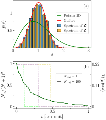
Figure 7: Limitations of the full level statistics approach in determining steady-state chaos. (a) Raw spectral statistics for the Liouvillian $\mathcal{L}$ and $\mathcal{L}^{\prime}$ defined in the main text. The green (red) curve is a guideline indicating an ideal 2D-Poisson (Ginibre) distribution. (b) As a function of time, the number of relevant eigenvalues $N_{\lambda}(t)$. Initially, $N_{\lambda}\simeq(N+1)^{2}$ for any quantum trajectory (dashed lines), i.e., all the Liouvillian eigenvalues are relevant. At random times, a quantum jump leads the system towards the stationary state $\ket{N}$ so that $N_{\lambda}=1$. This behaviour is captured by the average dynamics (solid line), and exactly matched by the indicator $\langle\cos(\theta)\rangle_{L}$ [we set $\langle\cos(\theta)\rangle_{L}=0$ when $N_{\lambda}=1$]. Parameters: $\beta=2$, $r=2$, $N=80$, and $g=$100\text{\,}\rm{arb.unit}$$ (defined with respect to the variance of the Gaussian ensemble from which the Hamiltonian is drawn), and $\forall m$ $\ket{\psi_{m}(0)}$ is chosen randomly within the Hilbert space.

As a general example, we consider random Liouvillians. Random Liouvillians are the generators of a class of completely-positive and trace-preserving maps, whose spectra match the universal predictions of non-Hermitian random matrix theory [37, 149, 42, 41, 49]. The procedure we adopt is the following:

• We construct a random Liouvillian $\mathcal{L}$ on a Hilbert space spanned by the orthornormal basis $\{\ket{0},\ket{1},\dots\ket{N-1}\}$. Following the procedure in Ref. [42], we define a basis for the operators in the Hilbert space $\{\hat{G}_{i}\}$ with $i=0,\ldots,N^{2}-1$ such that $\operatorname{Tr}[\hat{G}_{i}^{\dagger}\hat{G}_{j}]=\delta_{ij}$, with $\hat{G}_{0}=\hat{\mathbb{1}}/\sqrt{N}$. We construct $r$ jump operators as $\hat{L}_{\mu}=g\sum_{j=1}^{N^{2}-1}\hat{G}_{j}w_{j,\mu}$, with $\hat{L}_{\mu}$ traceless and $w$ a matrix sampled from a Ginibre ensemble. We then draw one instance of the Hamiltonian $\hat{H}$ from a Gaussian unitary ensemble, and define $\mathcal{L}$ according to Eq. (1).

• We determine the steady state $\hat{\rho}_{\rm ss}$ of this random Liouvillian and diagonalize it as $\hat{\rho}_{\rm ss}=\sum_{j}p_{j}\outerproduct{\Psi_{j}}{\Psi_{j}}$.

• We extend the Hilbert space to include a new state $\ket{N}$.

• We embed $\mathcal{L}$ into the larger Hilbert space, and construct the new Liouvillian $\mathcal{L}^{\prime}=\mathcal{L}+\mathcal{D}[\outerproduct{N}{\Psi_{0}}]$, where $\ket{\Psi_{0}}$ is the most probable eigenstate of $\hat{\rho}_{\rm ss}$. The new steady state is $\hat{\rho}_{\rm ss}^{\prime}=\outerproduct{N}{N}$ by construction.

The Liouvillian $\mathcal{L}^{\prime}$ defines a completely-positive and trace-preserving map. In Figure 7(a) we display its bulk statistics alongside that of $\mathcal{L}$. Both $\mathcal{L}$ and $\mathcal{L}^{\prime}$ follow a Ginibre distribution with only the former allowing for steady-state chaos. While the spectral statistics is unable to capture the steady-state properties of $\mathcal{L}^{\prime}$, we show in Fig. 7(b) that the SSQT criterion manages to correctly describe its transient chaotic dynamics giving way to an integrable steady state. We also signal the efficiency of the method in capturing these features using a limited number of quantum trajectories.

Notice that this procedure is general, can be extended to non-random Liouvillians, and that the Hilbert space extension can include more than one state. From a physical perspective, this mathematical construction is a particular instance of dissipative quantum state engineering [7], where the dynamics of an open quantum system is confined within a small portion of the Hilbert space.

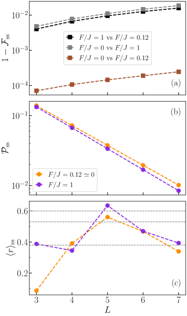
Figure 8: Limitations of a steady-state density matrix analysis in a coherently-driven open spin chain. (a) Fidelity $\mathcal{F}(\rho,\sigma)=\left(\operatorname{Tr}\sqrt{\sqrt{\rho}\sigma\sqrt{\rho}}\right)^{2}$ between the steady states of the three configurations $F/J=0$, $F/J=0.12$, and $F/J=1$ for increasing system size $L$. (b) As a function of $L$, the purity $\mathcal{P}_{\rm ss}=\Tr{\hat{\rho}_{\rm ss}^{2}}$ for the three configurations (the cases $F/J=0$ and $F/J=0.12$ overlap within this graphical resolution). (c) As a function of $L$, the quantifier $\langle r\rangle_{\rm ss}$. Parameters: $\gamma/J=1$, $\gamma_{1}^{+}/J=1$, $\gamma_{1}^{-}/J=0.8$, $\gamma_{L}^{+}/J=0.5$, $\gamma_{L}^{-}/J=1.2$.

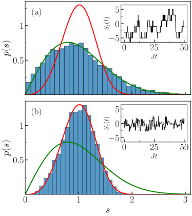
Figure 9: Relevant spectral statistics obtained applying the SSQT criterion on the coherently-driven open spin chain. (a) $F/J=0.12$. (b) $F/J=1$. The insets show the total spin $S_{z}=\sum_{j}\langle\hat{\sigma}_{j}^{z}\rangle$ along single quantum trajectories. The green (red) curve is a guideline indicating an ideal 2D-Poisson (Ginibre) distribution. Parameters: same as in Fig. 8 and $L=7$.

B.2 Entanglement spectrum and analysis of the steady state

We argue here that the structure of the steady-state density matrix $\hat{\rho}_{\rm ss}$ does not provide enough information about steady-state dynamics.

A possible diagnostic of regularity and chaos in the steady state, applied instead of the spectral statistics of the Liouvillian, has been discussed in Refs. [42, 41, 49] for the study of random Liouvillians and random Kraus maps. One formally defines the effective Hamiltonian

$$\hat{H}_{\rm ss}=-\log\left(\hat{\rho}_{\rm ss}\right),$$ (27)

and studies the statistical distribution of its eigenvalue spacing. In particular, an indicator is the Hamiltonian ratio $\langle r\rangle_{\rm ss}$ of $\hat{H}_{\rm ss}$ [c.f. Eq. (40)]. It ranges from $\langle r\rangle_{\rm ss}=0.38$, the ratio of a 1D Poisson distribution corresponding to an integrable Hamiltonian system, to $\langle r\rangle_{\rm ss}=0.60$, the ratio of a Gaussian Unitary Ensemble distribution characterizing a chaotic Hamiltonian system.

The model we consider is a 1D chain of $L$ two-level systems, whose Hamiltonian reads

$$\hat{H}=J\sum_{j=1}^{L-1}\left(\hat{\sigma}_{j}^{x}\hat{\sigma}_{j+1}^{x}+\hat{\sigma}_{j}^{y}\hat{\sigma}_{j+1}^{y}+\Delta\hat{\sigma}_{j}^{z}\hat{\sigma}_{j+1}^{z}\right)+F\sum_{j=1}^{L}\hat{\sigma}_{j}^{x}$$ (28)

where $\hat{\sigma}_{j}^{x,\,y,\,z}$ are the Pauli matrices. The presence of a drive $F$ generalizes the model introduced in Refs. [36, 40]. The system is subject to bulk dephasing of all spins and amplitude damping and gain at the boundaries. The Liouvillian reads

$$\begin{split}\mathcal{L}\hat{\rho}=&-i[\hat{H},\hat{\rho}]+\sum_{j}\gamma\mathcal{D}[\hat{\sigma}_{j}^{z}]\hat{\rho}\\ &\quad+\left(\gamma_{1}^{+}\mathcal{D}[\hat{\sigma}_{1}^{+}]+\gamma_{1}^{-}\mathcal{D}[\hat{\sigma}_{1}^{-}]\right)\hat{\rho}\\ &\quad+\left(\gamma_{L}^{+}\mathcal{D}[\hat{\sigma}_{L}^{+}]+\gamma_{L}^{-}\mathcal{D}[\hat{\sigma}_{L}^{-}]\right)\hat{\rho}\end{split}$$ (29)

We investigate the model at different intensities of the drive amplitude: $F/J=0$ (no drive), $F/J=0.12$ (weak drive), $F/J=1$ (strong drive). As shown in Fig. 8(a), the steady state changes only marginally in the three regimes. Furthermore, as displayed in Fig. 8(b), the steady state becomes only slightly more mixed upon increasing the drive amplitude. As such we conclude that methods based on the steady state alone should not observe significant differences between the three cases. This is indeed confirmed in Fig. 8(c), where the parameter $\langle r\rangle_{\rm ss}$ is displayed as a function of the system size [c.f. Eq. (27) and the discussion below].

From Fig. 8(c) we also deduce the unreliability of $\langle r\rangle_{\rm ss}$ as a model-independent predictor of DQC. In particular, for $F=0$ the model is known to be Bethe-ansatz integrable for all $L$ [36, 40] contrary to the predictions of $\langle r\rangle_{\rm ss}$ which varies with $L$ between integrability and chaos. The same dependence of $\langle r\rangle_{\rm ss}$ on $L$ also occurs for $F/J=0.12$ ($F/J=1$), whereas the spectral statistics criterion always predicts integrability (chaos).

We show in Fig. 9 that the SSQT criterion consistently characterizes all three configurations. In spite of the results in Fig. 8(b), for $F=0$ and $F/J=0.12$ the relevant level statistics is 2D Poissonian [c.f. Fig. 9(a)], while for $F/J=1$ it follows the Ginibre distribution [c.f. Fig. 9(b)]. Although only the case $L=7$ is shown, these predictions hold for all values of $L$. We also notice the profound difference between single quantum trajectories for $F/J=0.12$ and $F/J=1$, shown as insets to Fig. 9. This analysis demonstrates the effectiveness of our criterion in characterizing the dynamical properties of single trajectories, which ultimately determine the chaotic nature of the system.

B.3 Out-of-time-order correlators

Out-of-time order correlators (OTOCs) are a popular probe of chaotic dynamics in quantum systems [150, 151, 152]. Indeed, in the presence of chaotic behavior, OTOCs diverge and thus signal the presence of chaos [153]. Rapid exponential growth is associated with a quantum Lyapunov exponent, while the reached bound is often called the “bound on chaos” [150]. In non-chaotic systems, OTOCs usually display a linear or sub-linear initial growth.

Despite being a “necessary” condition for quantum chaos, OTOCs may be also diverging in non-chaotic settings. OTOCs measure scrambling in the system, i.e., the spread of local information in quantum systems. Although scrambling and chaos are often concomitant, recently the idea that scrambling implies chaos has been questioned [154, 155, 156, 157]. Examples of exponentially-growing OTOCs even in the absence of quantum chaos have been shown to be caused by features such as isolated saddle points [156]. As such, the presence of scrambling and exponentially diverging OTOCs thus does not equate to chaos.

OTOCs have been extended to open quantum systems [158]. Whether decoherence can lead to similar mechanisms for which OTOCs can grow exponentially in integrable systems remains unclear.

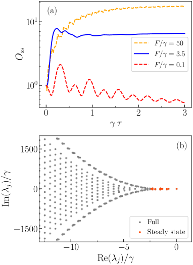
Figure 10: Ambiguity of out-of-time order correlators for the one-photon driven-dissipative Kerr resonator. (a) The OTOC defined in Eq. (30) calculated for the steady state $\hat{\rho}_{\rm ss}$ in the low photon regime ($F/\gamma=0.1$), close to the critical point ($F/\gamma=3.5$) and in the high photon regime ($F/\gamma=50$). While away from the critical point $O_{\rm ss}(\tau)$ correctly signals the integrability of the model, close to criticality, OTOC’s behavior becomes ambiguous. (b) For $F/\gamma=3.5$, the full Liouvillian spectrum is denoted by grey dots, and selected eigenvalues with the SSQT in the steady state are denoted by red dots. The SSQT analysis correctly predicts the model’s integrability. Other parameters are set to be $\Delta/\gamma=10$, $U/\gamma=10$.

Using the procedure detailed in, e.g., Ref. [1], we define

$$O_{t}(\tau)=-\langle[\hat{Q}(t+\tau),\hat{P}(t)]^{2}\rangle,$$ (30)

for $\hat{Q}(t)=[\hat{a}(t)+\hat{a}^{\dagger}(t)]/\sqrt{2}$ and $\hat{P}(t)=i[\hat{a}^{\dagger}(t)-\hat{a}(t)]/\sqrt{2}$, where $\hat{a}(t)$ is the annihilation operator in the Heisenberg picture. To evaluate the OTOCs, one can either use the master equation or quantum trajectories (with the prescription for evaluating correlation functions given in Ref. [91], see also [44]). We follow the first approach, adopting the procedure described in Ref. [1] for the computation of general correlations in open quantum systems. The OTOC can be written as:

$$O_{t}(\tau)=-(\langle\hat{Q}(t+\tau)\hat{P}(t)\hat{Q}(t+\tau)\hat{P}(t)\rangle$$ (31)

$$+\langle\hat{P}(t)\hat{Q}(t+\tau)\hat{P}(t)\hat{Q}(t+\tau)\rangle$$

$$-\langle\hat{Q}(t+\tau)\hat{P}(t)\hat{P}(t)\hat{Q}(t+\tau)\rangle$$

$$-\langle\hat{P}(t)\hat{Q}(t+\tau)\hat{Q}(t+\tau)\hat{P}(t)\rangle)$$

We start from a given initial density matrix $\hat{\rho}_{\rm in}$ and perform forward and “backward” time evolution solving the master equation with ${\hat{H}}$ and $-{\hat{H}}$ respectively (assuming the same jump operators for both time directions). We introduce the superoperators $\mathcal{F}_{O}\hat{\rho}=\hat{O}\hat{\rho}\hat{O}$, $\mathcal{F}_{O}^{R}\hat{\rho}=\hat{O}\hat{\rho}$, $\mathcal{F}_{O}^{L}\hat{\rho}=\hat{\rho}\hat{O}$, and the time evolution superoperator $V(t,0)\hat{\rho}$, with $V(t,0)\equiv\exp{(\mathcal{L}t)}$. Then, each term in the OTOC can be explicitly rewritten as

$$\langle\hat{Q}(t+\tau)\hat{P}(t)\hat{Q}(t+\tau)\hat{P}(t)\rangle=$$ (32)

$$\Tr{\mathcal{F}_{P}^{R}V(t,t+\tau)\mathcal{F}_{Q}V(t+\tau,t)\mathcal{F}_{P}^{R}V(t,0)\hat{\rho}_{\rm in}},$$

$$\langle\hat{P}(t)\hat{Q}(t+\tau)\hat{P}(t)\hat{Q}(t+\tau)\rangle=$$ (33)

$$\Tr{\mathcal{F}_{P}^{R}V(t,t+\tau)\mathcal{F}_{Q}V(t+\tau,t)\mathcal{F}_{P}^{L}V(t,0)\hat{\rho}_{\rm in}},$$

$$\hat{Q}(t+\tau)\hat{P}(t)\hat{P}(t)\hat{Q}(t+\tau)\rangle=$$ (34)

$$\Tr{\mathcal{F}_{P}V(t,t+\tau)\mathcal{F}_{Q}V(t+\tau,0)\hat{\rho}_{\rm in}},$$

$$\hat{P}(t)\hat{Q}(t+\tau)\hat{Q}(t+\tau)\hat{P}(t)\rangle=$$ (35)

$$\Tr{\mathcal{F}_{Q}V(t+\tau,t)\mathcal{F}_{P}V(t,0)\hat{\rho}_{\rm in}}.$$

The OTOC $O_{\rm ss}(\tau)\equiv\lim_{t\to\infty}O_{t}(\tau)$ is obtained by setting $\hat{\rho}_{\rm in}=\hat{\rho}_{ss}$.

Here we provide an example of two ambiguous behaviors of OTOCs in open systems. The first model we consider is the one-photon driven-dissipative Kerr resonator whose Hamiltonian reads

$$\hat{H}=-\Delta\hat{a}^{\dagger}\hat{a}+\frac{1}{2}U\hat{a}^{\dagger}\hat{a}^{\dagger}\hat{a}\hat{a}+F(\hat{a}^{\dagger}+\hat{a}),$$ (36)

with Lindblad equation

$$\frac{\partial\hat{\rho}}{\partial t}=-i[\hat{H},\hat{\rho}]+\gamma\left(\hat{a}\hat{\rho}\hat{a}^{\dagger}-\frac{1}{2}\anticommutator{\hat{a}^{\dagger}\hat{a}}{\hat{\rho}}\right).$$ (37)

The model is known to exhibit a first-order dissipative phase transition in the thermodynamic limit for a critical drive amplitude [19], and its steady state can be computed analytically [159, 160, 14]. The order parameter (in this case the photon number $n=\langle\hat{a}^{\dagger}\hat{a}\rangle$) abruptly jumps from zero to a finite value. Close to criticality, the system displays bistability, switching between two fixed points, which is non-chaotic [159, 14].

In Fig. 10(a) we numerically show the behavior of the steady-state OTOC (30). Away from criticality, the OTOC predicts the model’s integrability, while close to the critical point, in the presence of optical bistability, OTOC’s behavior becomes ambiguous. Fig. 10(b) shows the full Liouvillian spectrum diagonalized for a cutoff $N_{c}=30$, which is manifestly regular. Integrability is confirmed by the SSQT criterion, which shows how only a few eigenvalues are involved in steady-state dynamics.

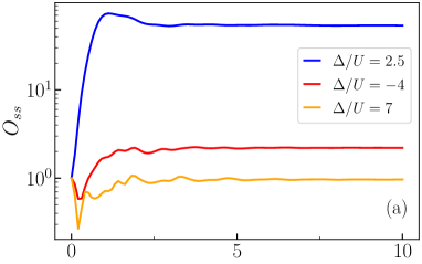
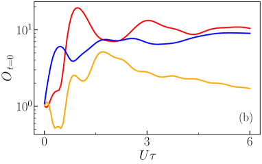
Figure 11: The OTOC defined in Eq. (30) calculated (a) at the steady state and (b) at $t=0$, for the driven-dissipative Bose-Hubbard model discussed in Sec. IV. The three selected configurations correspond to integrability ($\Delta/U=-4$), steady-state chaos ($\Delta/U=2.5$) and transient chaos ($\Delta/U=7$). The initial state in panel (b) is the coherent state $\ket{\psi(0)}=\ket{\alpha}\otimes\ket{\alpha}$ with $\alpha=2\sqrt{F/(\Delta-i\gamma)}$. The drive strength is $F/U=3$. Other parameters as in Fig. 2.

Finally, we demonstrate that OTOCs are also not predictive of transient chaos. Here, we consider the driven-dissipative Bose-Hubbard dimer discussed in Sec. IV Results are shown in Fig. 11. $O_{\rm ss}(\tau)$ rapidly increases only in the regions where the SSQT criterion predicts steady-state chaos [see Fig. 11(a)]. These findings support the results obtained in the main text. When we consider transient chaos, instead, we see that OTOCs are rather non-predictive [c.f. Fig. 11(b)]. For instance, a point characterized by both transient and steady-state DQC displays similar features with respect to one completely integrable. We thus conclude that OTOCs can be not capable of determining transient chaos in dissipative systems. We argue that the reason for this lack of correspondence is due to the exponential nature of the Liouvillian map, which may compensate for the diverging growth of the OTOC.

Appendix C Chaos in the Hamiltonian driven Bose-Hubbard model

Here, we characterize Hamiltonian quantum chaos in the boundary driven Bose-Hubbard model, whose Hamiltonian for an array of $N$ coupled nonlinear resonator reads

$$\begin{split}\hat{H}&=\sum_{j=1}^{N}\left(-\Delta\hat{a}_{j}^{\dagger}\hat{a}_{j}+\frac{1}{2}U\hat{a}_{j}^{\dagger}\hat{a}_{j}^{\dagger}\hat{a}_{j}\hat{a}_{j}\right)\\ &-J\sum_{j=1}^{N-1}\left(\hat{a}_{j+1}^{\dagger}\hat{a}_{j}+\hat{a}_{j}^{\dagger}\hat{a}_{j+1}\right)+F(\hat{a}_{1}^{\dagger}+\hat{a}_{1}),\end{split}$$ (38)

where $\hat{a}_{j}^{\dagger}$ and $\hat{a}_{j}$ are the bosonic creation and annihilation operators of the $j$-th cavity. The case $N=2$ thus corresponds to Eq. (13), and the limit where $\gamma=0$ in Eq. (14).

The goals of this analysis is to provide evidence for the importance of an energy cutoff in the analysis of the statistical distribution of eigenvalue spacings in non-$U(1)$ symmetric systems, and the inherent difficulty in setting this cutoff with physical criteria. We note, in passing, that the Hamiltonian problem with a driving term but no corresponding dissipation, is unphysical, as in typical experimental platforms if a channel is open for input, the same channel will also lead to a dissipation mechanism.

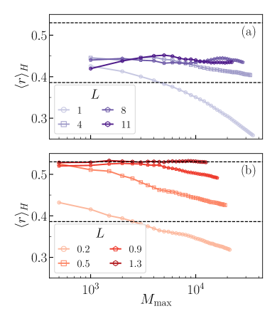
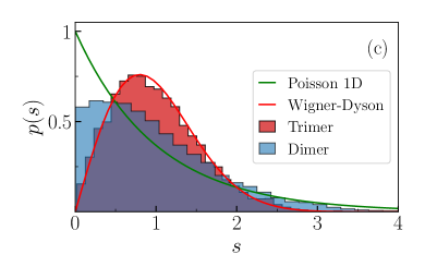
Figure 12: Chaos and integrability for the model Hamiltonian in Eq. (13). (a) For a dimer ($N=2$), the parameter $\langle r\rangle_{H}=\sum_{j=1}^{M_{\rm max}}r_{j}/M_{\rm max}$, for $r_{j}$ defined in (40), is plotted as a function of $M_{\rm max}$, for various values of the rescaling parameter $L$. (b) The same analysis as in (a), but for the case $N=3$. (c) The statistical distribution of energy-level distances for $N=2$ and $N=3$ and $L=11$ and $L=1.3$, respectively. Here $J/U=2$, $F/U=2.9$, $\Delta/U=2.5$.

As discussed above, to characterize quantum chaos in the Hamiltonian case we turn to the analysis of the spectral properties of the Hamiltonian [54, 55]. In particular, for the time-reversal invariant Hamiltonian in Eq. (13), the statistical distribution of nearest-neighbour energy spacings, defined as

$$p(s)=\sum_{j}\delta(\xi_{j+1}-\xi_{j}-s),$$ (39)

is Poissonian in the integrable case [79] and recovers a Wigner-Dyson distribution in the presence of chaos. Here, $\xi_{j}=\eta(E_{j})$, where $E_{j}$ are the eigenenergies, and $\eta$ is a polynomial function determined as in Ref. [147] and detailed in App. A.1. The link between universal spectral distributions of random-matrix ensembles and quantum chaos has been reviewed in Ref. [55]. The same features are also captured by the single number indicator $\langle r\rangle_{H}$ [161], which does not require any unfolding procedure. Let $s_{j}=E_{j+1}-E_{j}$ be the $j$-th spacing. Then,

$$r_{j}=\frac{\min(s_{j},s_{j-1})}{\max(s_{j},s_{j-1})}$$ (40)

and $\langle r\rangle_{H}$ is the average of $r_{j}$. One finds $\langle r\rangle_{H}=0.386$ for the 1D Poisson distribution and $\langle r\rangle_{H}=0.53$ for the Wigner-Dyson distribution. Values of $\langle r\rangle_{H}$ between these two limits are a signature of a hybrid regime between integrability and chaos, which has been interpreted as the coexistence of two statistically independent subsets in the eigenspectrum [162, 163, 164, 165]. Systems with a regularly spaced eigenspectrum are exceptions to this criterion, which clearly applies only when the eigenvalues are distributed following a (pseudo)-random distribution. In particular, the single harmonic oscillator, even if integrable, exhibits a spectrum with constant spacing, leading to $\langle r\rangle_{H}=1$. Similarly, when considering $N$ driven and coupled anharmonic oscillators, the total occupation number is not conserved and cannot be used to restrict the spectral analysis to a sector at constant occupation [99]. Then the eigenenergies at large occupation numbers are dominated by the nonlinear term, while the driving term becomes negligible leading to asymptotically decoupled anharmonic oscillators. It is then straightforward to show that $r_{j}\sim 1/j$, leading to $\langle r\rangle_{H}\to 0$ if the average is taken over the spectrum. As shown below, the numerical analysis of $\langle r\rangle_{H}$ shows this behaviour in the limit of large cutoff. The presence of a driving field therefore introduces an issue in the characterization of quantum chaos from the eigenvalue statistics.

To solve this issue, in the Hamiltonian model, we introduce the energy cutoff $M_{\rm max}$, and compute the level statistics over the set $\{E_{j},j\leq M_{\rm max}\}$ . This procedure is justified by the fact that, for an initial state with energy $E_{in}=\langle\psi_{in}|\hat{H}|\psi_{in}\rangle$, the eigendecomposition of $\ket{\psi_{in}}$ yields $\ket{\psi_{in}}=\sum_{j}c_{j}\ket{\psi_{j}}$, with $\sum_{j}|c_{j}|^{2}=1$ and $\hat{H}\ket{\psi_{j}}=E_{j}\ket{\psi_{j}}$. Therefore $E_{in}=\sum_{j}|c_{j}|^{2}E_{j}$ and, under reasonable physical assumptions, the initial state has finite energy and relevant components only on eigenstates within a finite energy window.

For the Hamiltonian case, where the computational Hilbert space scales with $N_{c}$, numerical diagonalization can be reasonably performed for $N=2,3$. In the Liouvillian case, where the computational space scales with $N_{c}^{2}$, this extensive analysis of the spectral properties becomes computationally intractable beyond $N=2$ and for large cutoffs. Thanks to this computational advantage in the Hamiltonian case, we can study the eigenvalue statistics in thermodynamic limit of the model. The thermodynamic limit is defined through the scale transformation

$$(\alpha_{1},...,\alpha_{N})\rightarrow\left(\alpha_{1}\sqrt{L},...,\alpha_{N}\sqrt{L}\right),$$ (41)

$$\,\,\,\,\,U\rightarrow\frac{U}{L},\,\,\,\,\,F\rightarrow F\sqrt{L},$$

where $L$ is a positive real number. The thermodynamic limit is achieved when $F\rightarrow+\infty$ keeping $UF^{2}$ constant [167].

The value of $\langle r\rangle_{H}$ for the two coupled modes is plotted in Fig. 12 (a) for several values of $L$. For $L=1$, the spectral indicator $\langle r\rangle_{H}$ approaches values below $0.386$ as $M_{\rm max}$ is increased, as expected from the argument given above. The same behaviour is expected even for larger values of $L$. This corresponds to smaller values of $U$, and the system should therefore display the asymptotic decoupling at larger $M_{\rm{max}}$. The value of $\langle r\rangle_{H}$ relevant for assessing quantum chaos should be rather taken in the limit of small $M_{\rm max}$, provided this cutoff is still large enough to give a statistically significant number of eigenvalues. For the case $N=2$, this limit seems to correspond to a value of $\langle r\rangle_{H}=0.45$, thus intermediate between the two limiting values. We cannot exclude that, for other parameter values, the system may display the fully chaotic level statistics. However, a full analysis of the Hamiltonian case is beyond the scope of this work. In Fig. 12(c) we show the distribution of level spacings for the unfolded spectrum compared to the 1D Poisson and the Wigner-Dyson distribution, again displaying an intermediate feature.

The value of $\langle r\rangle_{H}$ for $N=3$ is plotted in Fig. 12(b) for several values of $L$, with the same parameters as in Fig. 12(a). Again, for small values of $L$, the ratio decreases below $0.386$ as the cutoff is increased, as a result of the asymptotic decoupling anomaly. In this case of three coupled modes however, smaller values of the cutoff $M_{\rm max}$ clearly signal the universal signature of quantum chaos, with $\langle r\rangle_{H}$ approaching the value 0.53 associated with the Wigner-Dyson distribution. Correspondingly, the distribution of level spacings for the unfolded spectrum displayed in Fig. 12(c) also coincides with the fully chaotic Wigner-Dyson distribution.

References

- Breuer and Petruccione [2007] H.-P. Breuer and F. Petruccione, The Theory of Open Quantum Systems, 1st ed. (Oxford University PressOxford, 2007).
- Rivas and Huelga [2012] A. Rivas and S. F. Huelga, Open Quantum Systems: An Introduction, SpringerBriefs in Physics (Springer Berlin Heidelberg, Berlin, Heidelberg, 2012).
- Witthaut et al. [2008] D. Witthaut, F. Trimborn, and S. Wimberger, Dissipation induced coherence of a two-mode bose-einstein condensate, Physical Review Letters 101, 200402 (2008).
- Diehl et al. [2008] S. Diehl, A. Micheli, A. Kantian, B. Kraus, H. P. Büchler, and P. Zoller, Quantum states and phases in driven open quantum systems with cold atoms, Nature Physics 4, 878 (2008).
- Polkovnikov et al. [2011] A. Polkovnikov, K. Sengupta, A. Silva, and M. Vengalattore, Colloquium: Nonequilibrium dynamics of closed interacting quantum systems, Reviews of Modern Physics 83, 863 (2011).
- Eisert et al. [2015] J. Eisert, M. Friesdorf, and C. Gogolin, Quantum many-body systems out of equilibrium, Nature Physics 11, 124 (2015).
- Verstraete et al. [2009] F. Verstraete, M. M. Wolf, and J. I. Cirac, Quantum computation and quantum-state engineering driven by dissipation, Nature Physics 5, 633 (2009).
- Leghtas et al. [2015] Z. Leghtas, S. Touzard, I. M. Pop, A. Kou, B. Vlastakis, A. Petrenko, K. M. Sliwa, A. Narla, S. Shankar, M. J. Hatridge, M. Reagor, L. Frunzio, R. J. Schoelkopf, M. Mirrahimi, and M. H. Devoret, Confining the state of light to a quantum manifold by engineered two-photon loss, Science 347, 853 (2015).
- Touzard et al. [2018] S. Touzard, A. Grimm, Z. Leghtas, S. O. Mundhada, P. Reinhold, C. Axline, M. Reagor, K. Chou, J. Blumoff, K. M. Sliwa, S. Shankar, L. Frunzio, R. J. Schoelkopf, M. Mirrahimi, and M. H. Devoret, Coherent oscillations inside a quantum manifold stabilized by dissipation, Physical Review X 8, 021005 (2018).
- Chamberland et al. [2022] C. Chamberland, K. Noh, P. Arrangoiz-Arriola, E. T. Campbell, C. T. Hann, J. Iverson, H. Putterman, T. C. Bohdanowicz, S. T. Flammia, A. Keller, G. Refael, J. Preskill, L. Jiang, A. H. Safavi-Naeini, O. Painter, and F. G. Brandão, Building a fault-tolerant quantum computer using concatenated cat codes, PRX Quantum 3, 010329 (2022).
- Lescanne et al. [2020] R. Lescanne, M. Villiers, T. Peronnin, A. Sarlette, M. Delbecq, B. Huard, T. Kontos, M. Mirrahimi, and Z. Leghtas, Exponential suppression of bit-flips in a qubit encoded in an oscillator, Nature Physics 16, 509 (2020).
- Carusotto and Ciuti [2013] I. Carusotto and C. Ciuti, Quantum fluids of light, Reviews of Modern Physics 85, 299 (2013).
- Carmichael [2015] H. Carmichael, Breakdown of Photon Blockade: A Dissipative Quantum Phase Transition in Zero Dimensions, Physical Review X 5, 031028 (2015).
- Bartolo et al. [2016] N. Bartolo, F. Minganti, W. Casteels, and C. Ciuti, Exact steady state of a Kerr resonator with one- and two-photon driving and dissipation: Controllable Wigner-function multimodality and dissipative phase transitions, Physical Review A 94, 033841 (2016).
- Macieszczak et al. [2016] K. Macieszczak, M. Guţă, I. Lesanovsky, and J. P. Garrahan, Towards a Theory of Metastability in Open Quantum Dynamics, Physical Review Letters 116, 240404 (2016).
- Fink et al. [2017] J. Fink, A. Dombi, A. Vukics, A. Wallraff, and P. Domokos, Observation of the Photon-Blockade Breakdown Phase Transition, Physical Review X 7, 011012 (2017).
- Fitzpatrick et al. [2017] M. Fitzpatrick, N. M. Sundaresan, A. C. Li, J. Koch, and A. A. Houck, Observation of a Dissipative Phase Transition in a One-Dimensional Circuit QED Lattice, Physical Review X 7, 011016 (2017).
- Biondi et al. [2017] M. Biondi, G. Blatter, H. E. Türeci, and S. Schmidt, Nonequilibrium gas-liquid transition in the driven-dissipative photonic lattice, Physical Review A 96, 043809 (2017).
- Minganti et al. [2018] F. Minganti, A. Biella, N. Bartolo, and C. Ciuti, Spectral theory of liouvillians for dissipative phase transitions, Phys. Rev. A 98, 042118 (2018).
- Fink et al. [2018] T. Fink, A. Schade, S. Höfling, C. Schneider, and A. Imamoglu, Signatures of a dissipative phase transition in photon correlation measurements, Nature Physics 14, 365 (2018).
- Di Candia et al. [2023] R. Di Candia, F. Minganti, K. V. Petrovnin, G. S. Paraoanu, and S. Felicetti, Critical parametric quantum sensing, npj Quantum Information 9, 23 (2023).
- Gravina et al. [2023] L. Gravina, F. Minganti, and V. Savona, Critical schrödinger cat qubit, PRX Quantum 4, 020337 (2023).
- Grimsmo and Puri [2021] A. L. Grimsmo and S. Puri, Quantum Error Correction with the Gottesman-Kitaev-Preskill Code, PRX Quantum 2, 020101 (2021).
- Hillmann et al. [2022] T. Hillmann, F. Quijandría, A. L. Grimsmo, and G. Ferrini, Performance of Teleportation-Based Error-Correction Circuits for Bosonic Codes with Noisy Measurements, PRX Quantum 3, 020334 (2022).
- Lidar et al. [1998] D. A. Lidar, I. L. Chuang, and K. B. Whaley, Decoherence-free subspaces for quantum computation, Physical Review Letters 81, 2594 (1998).
- Knill et al. [2000] E. Knill, R. Laflamme, and L. Viola, Theory of quantum error correction for general noise, Physical Review Letters 84, 2525 (2000).
- Albert et al. [2016] V. V. Albert, B. Bradlyn, M. Fraas, and L. Jiang, Geometry and response of lindbladians, Physical Review X 6, 041031 (2016).
- Lidar [2014] D. A. Lidar, Review of decoherence-free subspaces, noiseless subsystems, and dynamical decoupling, in Advances in Chemical Physics, Advances in chemical physics (John Wiley & Sons, Inc., Hoboken, New Jersey, 2014) pp. 295–354.
- Kempe et al. [2001] J. Kempe, D. Bacon, D. A. Lidar, and K. B. Whaley, Theory of decoherence-free fault-tolerant universal quantum computation, Physical Review A 63, 042307 (2001).
- Gong et al. [2018] Z. Gong, Y. Ashida, K. Kawabata, K. Takasan, S. Higashikawa, and M. Ueda, Topological Phases of Non-Hermitian Systems, Physical Review X 8, 031079 (2018).
- Kawabata et al. [2019] K. Kawabata, K. Shiozaki, M. Ueda, and M. Sato, Symmetry and Topology in Non-Hermitian Physics, Physical Review X 9, 041015 (2019).
- Hamazaki et al. [2019] R. Hamazaki, K. Kawabata, and M. Ueda, Non-Hermitian Many-Body Localization, Physical Review Letters 123, 090603 (2019).
- Ippoliti et al. [2021] M. Ippoliti, M. J. Gullans, S. Gopalakrishnan, D. A. Huse, and V. Khemani, Entanglement Phase Transitions in Measurement-Only Dynamics, Physical Review X 11, 011030 (2021).
- Hamazaki et al. [2022] R. Hamazaki, M. Nakagawa, T. Haga, and M. Ueda, Lindbladian Many-Body Localization (2022), arXiv:2206.02984 [quant-ph] .
- Kawabata et al. [2023a] K. Kawabata, T. Numasawa, and S. Ryu, Entanglement Phase Transition Induced by the Non-Hermitian Skin Effect, Physical Review X 13, 021007 (2023a).
- Akemann et al. [2019] G. Akemann, M. Kieburg, A. Mielke, and T. Prosen, Universal Signature from Integrability to Chaos in Dissipative Open Quantum Systems, Physical Review Letters 123, 254101 (2019).
- Denisov et al. [2019] S. Denisov, T. Laptyeva, W. Tarnowski, D. Chruściński, and K. Życzkowski, Universal Spectra of Random Lindblad Operators, Physical Review Letters 123, 140403 (2019).
- Can et al. [2019] T. Can, V. Oganesyan, D. Orgad, and S. Gopalakrishnan, Spectral Gaps and Midgap States in Random Quantum Master Equations, Physical Review Letters 123, 234103 (2019).
- Hamazaki et al. [2020] R. Hamazaki, K. Kawabata, N. Kura, and M. Ueda, Universality classes of non-Hermitian random matrices, Physical Review Research 2, 023286 (2020).
- Sá et al. [2020a] L. Sá, P. Ribeiro, and T. Prosen, Complex Spacing Ratios: A Signature of Dissipative Quantum Chaos, Physical Review X 10, 021019 (2020a).
- Sá et al. [2020b] L. Sá, P. Ribeiro, T. Can, and T. Prosen, Spectral transitions and universal steady states in random Kraus maps and circuits, Physical Review B 102, 134310 (2020b).
- Sá et al. [2020c] L. Sá, P. Ribeiro, and T. Prosen, Spectral and steady-state properties of random liouvillians, Journal of Physics A: Mathematical and Theoretical 53, 305303 (2020c).
- Li et al. [2021] J. Li, T. Prosen, and A. Chan, Spectral Statistics of Non-Hermitian Matrices and Dissipative Quantum Chaos, Physical Review Letters 127, 170602 (2021).
- Dahan et al. [2022] D. Dahan, G. Arwas, and E. Grosfeld, Classical and quantum chaos in chirally-driven, dissipative Bose-Hubbard systems, npj Quantum Information 8, 14 (2022).
- Rubio-García et al. [2022] A. Rubio-García, R. Molina, and J. Dukelsky, From integrability to chaos in quantum Liouvillians, SciPost Physics Core 5, 026 (2022).
- Prasad et al. [2022] M. Prasad, H. K. Yadalam, C. Aron, and M. Kulkarni, Dissipative quantum dynamics, phase transitions, and non-Hermitian random matrices, Physical Review A 105, L050201 (2022).
- García-García et al. [2022] A. M. García-García, L. Sá, and J. J. Verbaarschot, Symmetry Classification and Universality in Non-Hermitian Many-Body Quantum Chaos by the Sachdev-Ye-Kitaev Model, Physical Review X 12, 021040 (2022).
- Kolovsky [2022] A. R. Kolovsky, Bistability and chaos-assisted tunneling in dissipative quantum systems, Physical Review E 106, 014209 (2022).
- Costa et al. [2023] J. Costa, P. Ribeiro, A. D. Luca, T. Prosen, and L. Sá, Spectral and steady-state properties of fermionic random quadratic Liouvillians, SciPost Physics 15, 145 (2023).
- Sá et al. [2023] L. Sá, P. Ribeiro, and T. Prosen, Symmetry Classification of Many-Body Lindbladians: Tenfold Way and Beyond, Physical Review X 13, 031019 (2023).
- Kawabata et al. [2023b] K. Kawabata, A. Kulkarni, J. Li, T. Numasawa, and S. Ryu, Symmetry of open quantum systems: Classification of dissipative quantum chaos, PRX Quantum 4, 030328 (2023b).
- Kawabata et al. [2023c] K. Kawabata, Z. Xiao, T. Ohtsuki, and R. Shindou, Singular-value statistics of non-hermitian random matrices and open quantum systems, PRX Quantum 4, 040312 (2023c).
- Matsoukas-Roubeas et al. [2023] A. S. Matsoukas-Roubeas, T. Prosen, and A. del Campo, Quantum Chaos and Coherence: Random Parametric Quantum Channels (2023), arXiv:2305.19326 [quant-ph] .
- Haake [2001] F. Haake, Quantum Signatures of Chaos, edited by H. Haken, Springer Series in Synergetics, Vol. 54 (Springer Berlin Heidelberg, Berlin, Heidelberg, 2001).
- D’Alessio et al. [2016] L. D’Alessio, Y. Kafri, A. Polkovnikov, and M. Rigol, From quantum chaos and eigenstate thermalization to statistical mechanics and thermodynamics, Advances in Physics 65, 239 (2016).
- Lindblad [1976] G. Lindblad, On the generators of quantum dynamical semigroups, Communications in Mathematical Physics 48, 119 (1976).
- Grobe et al. [1988] R. Grobe, F. Haake, and H.-J. Sommers, Quantum Distinction of Regular and Chaotic Dissipative Motion, Physical Review Letters 61, 1899 (1988).
- Note [1] If the Hilbert space is finite and the Liouvillian superoperator is time-independent, the existence of at least one steady state is guaranteed [2]. If the system is not invariant under any strong Liouvillian symmetry, the steady state is also unique [111]. In this work, we consider open quantum systems admitting a unique steady state.
- Wiseman and Milburn [2009] H. M. Wiseman and G. J. Milburn, Quantum Measurement and Control, 1st ed. (Cambridge University Press, 2009).
- Jacobs [2014] K. Jacobs, Quantum Measurement Theory and its Applications (Cambridge University Press, 2014).
- Daley [2014] A. J. Daley, Quantum trajectories and open many-body quantum systems, Advances in Physics 63, 77 (2014).
- Weimer et al. [2021] H. Weimer, A. Kshetrimayum, and R. Orús, Simulation methods for open quantum many-body systems, Reviews of Modern Physics 93, 015008 (2021).
- Georgescu et al. [2014] I. M. Georgescu, S. Ashhab, and F. Nori, Quantum simulation, Review of Modern Physics 86, 153 (2014).
- Hur et al. [2016] K. L. Hur, L. Henriet, A. Petrescu, K. Plekhanov, G. Roux, and M. Schiró, Many-body quantum electrodynamics networks: Non-equilibrium condensed matter physics with light, Comptes Rendus Physique 17, 808 (2016).
- Altman et al. [2021] E. Altman, K. R. Brown, G. Carleo, L. D. Carr, E. Demler, C. Chin, B. DeMarco, S. E. Economou, M. A. Eriksson, K.-M. C. Fu, M. Greiner, K. R. Hazzard, R. G. Hulet, A. J. Kollár, B. L. Lev, M. D. Lukin, R. Ma, X. Mi, S. Misra, C. Monroe, K. Murch, Z. Nazario, K.-K. Ni, A. C. Potter, P. Roushan, M. Saffman, M. Schleier-Smith, I. Siddiqi, R. Simmonds, M. Singh, I. Spielman, K. Temme, D. S. Weiss, J. Vučković, V. Vuletić, J. Ye, and M. Zwierlein, Quantum Simulators: Architectures and Opportunities, PRX Quantum 2, 017003 (2021).
- Krantz et al. [2019] P. Krantz, M. Kjaergaard, F. Yan, T. P. Orlando, S. Gustavsson, and W. D. Oliver, A quantum engineer’s guide to superconducting qubits, Applied Physics Reviews 6, 021318 (2019).
- Blais et al. [2021] A. Blais, A. L. Grimsmo, S. Girvin, and A. Wallraff, Circuit quantum electrodynamics, Reviews of Modern Physics 93, 025005 (2021).
- Burkard et al. [2020] G. Burkard, M. J. Gullans, X. Mi, and J. R. Petta, Superconductor–semiconductor hybrid-circuit quantum electrodynamics, Nature Reviews Physics 2, 129 (2020).
- García De Arquer et al. [2021] F. P. García De Arquer, D. V. Talapin, V. I. Klimov, Y. Arakawa, M. Bayer, and E. H. Sargent, Semiconductor quantum dots: Technological progress and future challenges, Science 373, eaaz8541 (2021).
- Aspelmeyer et al. [2014] M. Aspelmeyer, T. J. Kippenberg, and F. Marquardt, Cavity optomechanics, Reviews of Modern Physics 86, 1391 (2014).
- Müller et al. [2012] M. Müller, S. Diehl, G. Pupillo, and P. Zoller, Engineered Open Systems and Quantum Simulations with Atoms and Ions, in Advances In Atomic, Molecular, and Optical Physics, Vol. 61 (Elsevier, 2012) pp. 1–80.
- Bruzewicz et al. [2019] C. D. Bruzewicz, J. Chiaverini, R. McConnell, and J. M. Sage, Trapped-ion quantum computing: Progress and challenges, Applied Physics Reviews 6, 021314 (2019).
- Mirrahimi et al. [2014] M. Mirrahimi, Z. Leghtas, V. V. Albert, S. Touzard, R. J. Schoelkopf, L. Jiang, and M. H. Devoret, Dynamically protected cat-qubits: a new paradigm for universal quantum computation, New Journal of Physics 16, 045014 (2014).
- Puri et al. [2017] S. Puri, S. Boutin, and A. Blais, Engineering the quantum states of light in a Kerr-nonlinear resonator by two-photon driving, npj Quantum Information 3, 18 (2017).
- Puri et al. [2019] S. Puri, A. Grimm, P. Campagne-Ibarcq, A. Eickbusch, K. Noh, G. Roberts, L. Jiang, M. Mirrahimi, M. H. Devoret, and S. M. Girvin, Stabilized cat in a driven nonlinear cavity: A fault-tolerant error syndrome detector, Physical Review X 9, 041009 (2019).
- Gautier et al. [2022] R. Gautier, A. Sarlette, and M. Mirrahimi, Combined dissipative and hamiltonian confinement of cat qubits, PRX Quantum 3, 020339 (2022).
- Heugel et al. [2019] T. L. Heugel, M. Biondi, O. Zilberberg, and R. Chitra, Quantum transducer using a parametric driven-dissipative phase transition, Physical Review Letters 123, 173601 (2019).
- Rosenzweig and Porter [1960] N. Rosenzweig and C. E. Porter, ”Repulsion of Energy Levels” in Complex Atomic Spectra, Physical Review 120, 1698 (1960).
- Berry and Tabor [1977] M. V. Berry and M. Tabor, Level clustering in the regular spectrum, Proceedings of the Royal Society of London. A. Mathematical and Physical Sciences 356, 375 (1977).
- Casati et al. [1980] G. Casati, F. Valz-Gris, and I. Guarnieri, On the connection between quantization of nonintegrable systems and statistical theory of spectra, Lettere al Nuovo Cimento 28, 279 (1980).
- Bohigas et al. [1984] O. Bohigas, M. J. Giannoni, and C. Schmit, Characterization of Chaotic Quantum Spectra and Universality of Level Fluctuation Laws, Physical Review Letters 52, 1 (1984).
- Dyson [1962] F. J. Dyson, The Threefold Way. Algebraic Structure of Symmetry Groups and Ensembles in Quantum Mechanics, Journal of Mathematical Physics 3, 1199 (1962).
- Berry [1985] M. V. Berry, Semiclassical theory of spectral rigidity, Proceedings of the Royal Society of London. A. Mathematical and Physical Sciences 400, 229 (1985).
- Sieber and Richter [2001] M. Sieber and K. Richter, Correlations between periodic orbits and their role in spectral statistics, Physica Scripta 2001, 128 (2001).
- Sieber [2002] M. Sieber, Leading off-diagonal approximation for the spectral form factor for uniformly hyperbolic systems, J. Phys. A 35, L613 (2002).
- Müller et al. [2004] S. Müller, S. Heusler, P. Braun, F. Haake, and A. Altland, Semiclassical foundation of universality in quantum chaos, Physical Review Letters 93, 014103 (2004).
- Müller et al. [2005] S. Müller, S. Heusler, P. Braun, F. Haake, and A. Altland, Periodic-orbit theory of universality in quantum chaos, Physical Review E 72, 046207 (2005).
- Kos et al. [2018] P. Kos, M. Ljubotina, and T. c. v. Prosen, Many-body quantum chaos: Analytic connection to random matrix theory, Physical Review X 8, 021062 (2018).
- Gorini et al. [1976] V. Gorini, A. Kossakowski, and E. C. G. Sudarshan, Completely positive dynamical semigroups of -level systems, Journal of Mathematical Physics 17, 821 (1976).
- Markum et al. [1999] H. Markum, R. Pullirsch, and T. Wettig, Non-Hermitian Random Matrix Theory and Lattice QCD with Chemical Potential, Physical Review Letters 83, 484 (1999).
- Mølmer et al. [1993] K. Mølmer, Y. Castin, and J. Dalibard, Monte Carlo wave-function method in quantum optics, Journal of the Optical Society of America B 10, 524 (1993).
- Carmichael [1993] H. Carmichael, An Open Systems Approach to Quantum Optics: Lectures Presented at the Université Libre de Bruxelles October 28 to November 4, 1991, edited by H. Araki, E. Brézin, J. Ehlers, U. Frisch, K. Hepp, R. L. Jaffe, R. Kippenhahn, H. A. Weidenmüller, J. Wess, J. Zittartz, and W. Beiglböck, Lecture Notes in Physics Monographs, Vol. 18 (Springer Berlin Heidelberg, Berlin, Heidelberg, 1993).
- Gardiner and Zoller [2000] C. W. Gardiner and P. Zoller, Quantum Noise, 2nd ed., edited by H. Haken (Springer, 2000).
- Chen et al. [2023] Q.-M. Chen, M. Fischer, Y. Nojiri, M. Renger, E. Xie, M. Partanen, S. Pogorzalek, K. G. Fedorov, A. Marx, F. Deppe, and R. Gross, Quantum behavior of the Duffing oscillator at the dissipative phase transition, Nature Communications 14, 2896 (2023).
- Beaulieu et al. [2023] G. Beaulieu, F. Minganti, S. Frasca, V. Savona, S. Felicetti, R. D. Candia, and P. Scarlino, Observation of first- and second-order dissipative phase transitions in a two-photon driven kerr resonator (2023), arXiv:2310.13636 [quant-ph] .
- Buchleitner and Kolovsky [2003] A. Buchleitner and A. R. Kolovsky, Interaction-induced decoherence of atomic bloch oscillations, Physical Review Letters 91, 253002 (2003).
- Kolovsky and Buchleitner [2004] A. R. Kolovsky and A. Buchleitner, Quantum chaos in the Bose-Hubbard model, Europhysics Letters (EPL) 68, 632 (2004).
- Tomadin et al. [2007] A. Tomadin, R. Mannella, and S. Wimberger, Many-body interband tunneling as a witness of complex dynamics in the bose-hubbard model, Physical Review Letters 98, 130402 (2007).
- Kollath et al. [2010] C. Kollath, G. Roux, G. Biroli, and A. M. Läuchli, Statistical properties of the spectrum of the extended Bose–Hubbard model, Journal of Statistical Mechanics: Theory and Experiment 2010, P08011 (2010).
- Parra-Murillo et al. [2013] C. A. Parra-Murillo, J. Madroñero, and S. Wimberger, Two-band bose-hubbard model for many-body resonant tunneling in the wannier-stark system, Physical Review A 88, 032119 (2013).
- Fischer et al. [2016] D. Fischer, D. Hoffmann, and S. Wimberger, Spectral analysis of two-dimensional bose-hubbard models, Physical Review A 93, 043620 (2016).
- Dubertrand and Müller [2016] R. Dubertrand and S. Müller, Spectral statistics of chaotic many-body systems, New Journal of Physics 18, 033009 (2016).
- Rautenberg and Gärttner [2020] M. Rautenberg and M. Gärttner, Classical and quantum chaos in a three-mode bosonic system, Physical Review A 101, 053604 (2020).
- De La Cruz et al. [2020] J. De La Cruz, S. Lerma-Hernández, and J. G. Hirsch, Quantum chaos in a system with high degree of symmetries, Physical Review E 102, 032208 (2020).
- Pausch et al. [2021] L. Pausch, E. G. Carnio, A. Rodríguez, and A. Buchleitner, Chaos and ergodicity across the energy spectrum of interacting bosons, Physical Review Letters 126, 150601 (2021).
- Goto and Kanao [2021] H. Goto and T. Kanao, Chaos in coupled Kerr-nonlinear parametric oscillators, Physical Review Research 3, 043196 (2021).
- Pausch et al. [2022] L. Pausch, A. Buchleitner, E. G. Carnio, and A. Rodríguez, Optimal route to quantum chaos in the Bose–Hubbard model, J. Phys. A 55, 324002 (2022).
- Minganti et al. [2019] F. Minganti, A. Miranowicz, R. W. Chhajlany, and F. Nori, Quantum exceptional points of non-Hermitian Hamiltonians and Liouvillians: The effects of quantum jumps, Physical Review A 100, 062131 (2019).
- Note [2] Different unravelings, correspond to different types of measurements. Among the most common unravelings are the homodyne measurement [92], resulting in a Wiener process for the system’s state , and the photon-counting measurement [91, 59], giving rise to the celebrated quantum jumps.
- Note [3] Since quantum trajectories in the unique steady state of an open quantum system are ergodic [95], one can also let a single quantum trajectory evolve towards the steady state and then sample the sets in time rather than in number of trajectories.
- Albert and Jiang [2014] V. V. Albert and L. Jiang, Symmetries and conserved quantities in Lindblad master equations, Physical Review A 89, 022118 (2014).
- Buča and Prosen [2012] B. Buča and T. Prosen, A note on symmetry reductions of the Lindblad equation: transport in constrained open spin chains, New Journal of Physics 14, 073007 (2012).
- Bartolo et al. [2017] N. Bartolo, F. Minganti, J. Lolli, and C. Ciuti, Homodyne versus photon-counting quantum trajectories for dissipative Kerr resonators with two-photon driving, The European Physical Journal Special Topics 226, 2705 (2017).
- Sánchez Muñoz et al. [2019] C. Sánchez Muñoz, B. Buča, J. Tindall, A. González-Tudela, D. Jaksch, and D. Porras, Symmetries and conservation laws in quantum trajectories: Dissipative freezing, Phys. Rev. A 100, 042113 (2019).
- Johansson et al. [2012] J. Johansson, P. Nation, and F. Nori, Qutip: An open-source python framework for the dynamics of open quantum systems, Computer Physics Communications 183, 1760 (2012).
- Johansson et al. [2013] J. Johansson, P. Nation, and F. Nori, Qutip 2: A python framework for the dynamics of open quantum systems, Computer Physics Communications 184, 1234 (2013).
- Note [4] The choice of a cavity cutoff ensures the convergence of the spectral statistics as proposed in [40] and [46]. We however note that with the proposed cutoff for some of the points in the phase diagram (in particular with ), expectation values have not yet reached convergence. This however does not change the spectral distinction between chaos and integrability.
- Note [5] A rigorous derivation of the semiclassical limit of the Lindblad master equation indicates that the correct classical limit, i.e. should include second-order correlations between fields [168]. Here we will identify the classical limit as the the mean-field approximation, which assumes that second-order correlators factor into field products.
- Casteels and Ciuti [2017] W. Casteels and C. Ciuti, Quantum entanglement in the spatial-symmetry-breaking phase transition of a driven-dissipative bose-hubbard dimer, Phys. Rev. A 95, 013812 (2017).
- Debnath et al. [2017] K. Debnath, E. Mascarenhas, and V. Savona, Nonequilibrium photonic transport and phase transition in an array of optical cavities, New Journal of Physics 19, 115006 (2017).
- Giraldo et al. [2020] A. Giraldo, B. Krauskopf, N. G. R. Broderick, J. A. Levenson, and A. M. Yacomotti, The driven-dissipative Bose–Hubbard dimer: phase diagram and chaos, New Journal of Physics 22, 043009 (2020).
- Strogatz [2018] S. H. Strogatz, Nonlinear Dynamics and Chaos, 0th ed. (CRC Press, 2018).
- Davidovich [1996] L. Davidovich, Sub-poissonian processes in quantum optics, Review of Modern Physics 68, 127 (1996).
- Misra and Sudarshan [1977] B. Misra and E. C. G. Sudarshan, The Zeno’s paradox in quantum theory, Journal of Mathematical Physics 18, 756 (1977).
- Walls and Milburn [2008] D. Walls and G. J. Milburn, eds., Quantum Optics (Springer Berlin Heidelberg, Berlin, Heidelberg, 2008).
- Jin et al. [2016] J. Jin, A. Biella, O. Viyuela, L. Mazza, J. Keeling, R. Fazio, and D. Rossini, Cluster mean-field approach to the steady-state phase diagram of dissipative spin systems, Physical Review X 6, 031011 (2016).
- Huybrechts and Wouters [2019] D. Huybrechts and M. Wouters, Cluster methods for the description of a driven-dissipative spin model, Physical Review A 99, 043841 (2019).
- Kubo [1962] R. Kubo, Generalized Cumulant Expansion Method, Journal of the Physical Society of Japan 17, 1100 (1962).
- Plankensteiner et al. [2022] D. Plankensteiner, C. Hotter, and H. Ritsch, QuantumCumulants.jl: A Julia framework for generalized mean-field equations in open quantum systems, Quantum 6, 617 (2022).
- Verstraelen et al. [2023] W. Verstraelen, D. Huybrechts, T. Roscilde, and M. Wouters, Quantum and classical correlations in open quantum spin lattices via truncated-cumulant trajectories, PRX Quantum 4, 030304 (2023).
- Hillery et al. [1984] M. Hillery, R. O’Connell, M. Scully, and E. Wigner, Distribution functions in physics: Fundamentals, Physics Reports 106, 121 (1984).
- Carmichael [1999] H. J. Carmichael, Statistical Methods in Quantum Optics 1 (Springer Berlin Heidelberg, Berlin, Heidelberg, 1999).
- Polkovnikov [2010] A. Polkovnikov, Phase space representation of quantum dynamics, Annals of Physics 325, 1790 (2010).
- Kordas et al. [2013] G. Kordas, S. Wimberger, and D. Witthaut, Decay and fragmentation in an open bose-hubbard chain, Physical Review A 87, 043618 (2013).
- Vicentini et al. [2018] F. Vicentini, F. Minganti, R. Rota, G. Orso, and C. Ciuti, Critical slowing down in driven-dissipative bose-hubbard lattices, Physical Review A 97, 013853 (2018).
- Schlagheck et al. [2019] P. Schlagheck, D. Ullmo, J. D. Urbina, K. Richter, and S. Tomsovic, Enhancement of many-body quantum interference in chaotic bosonic systems: The role of symmetry and dynamics, Physical Review Letters 123, 215302 (2019).
- Das et al. [2018] A. Das, S. Chakrabarty, A. Dhar, A. Kundu, D. A. Huse, R. Moessner, S. S. Ray, and S. Bhattacharjee, Light-cone spreading of perturbations and the butterfly effect in a classical spin chain, Physical Review Letters 121, 024101 (2018).
- Bilitewski et al. [2018] T. Bilitewski, S. Bhattacharjee, and R. Moessner, Temperature dependence of the butterfly effect in a classical many-body system, Phys. Rev. Lett. 121, 250602 (2018).
- Schuckert and Knap [2019] A. Schuckert and M. Knap, Many-body chaos near a thermal phase transition, SciPost Phys. 7, 022 (2019).
- Bilitewski et al. [2021] T. Bilitewski, S. Bhattacharjee, and R. Moessner, Classical many-body chaos with and without quasiparticles, Physical Review B 103, 174302 (2021).
- Ruidas and Banerjee [2021] S. Ruidas and S. Banerjee, Many-body chaos and anomalous diffusion across thermal phase transitions in two dimensions, SciPost Phys. 11, 087 (2021).
- Deger et al. [2022] A. Deger, S. Roy, and A. Lazarides, Arresting classical many-body chaos by kinetic constraints, Phys. Rev. Lett. 129, 160601 (2022).
- Mondal et al. [2023] D. Mondal, K. Sengupta, and S. Sinha, Emergence of a quasi-ergodic steady state in a dissipative tavis-cummings array (2023), arXiv:2310.12779 [cond-mat.stat-mech] .
- Berke et al. [2022] C. Berke, E. Varvelis, S. Trebst, A. Altland, and D. P. DiVincenzo, Transmon platform for quantum computing challenged by chaotic fluctuations, Nature Communications 13, 2495 (2022).
- Cohen et al. [2023] J. Cohen, A. Petrescu, R. Shillito, and A. Blais, Reminiscence of classical chaos in driven transmons, PRX Quantum 4, 020312 (2023).
- Chávez-Carlos et al. [2023] J. Chávez-Carlos, R. G. Cortiñas, M. A. P. Reynoso, I. García-Mata, V. S. Batista, F. Pérez-Bernal, D. A. Wisniacki, and L. F. Santos, Driving superconducting qubits into chaos (2023), arXiv:2310.17698 [quant-ph] .
- Guhr et al. [1998] T. Guhr, A. Müller–Groeling, and H. A. Weidenmüller, Random-matrix theories in quantum physics: common concepts, Physics Reports 299, 189 (1998).
- Sprott [2003] J. C. Sprott, Chaos and time-series analysis (Oxford University Press, Oxford ; New York, 2003).
- Can [2019] T. Can, Random Lindblad dynamics, Journal of Physics A: Mathematical and Theoretical 52, 485302 (2019).
- Maldacena et al. [2016] J. Maldacena, S. H. Shenker, and D. Stanford, A bound on chaos, Journal of High Energy Physics 2016, 106 (2016).
- Hashimoto et al. [2017] K. Hashimoto, K. Murata, and R. Yoshii, Out-of-time-order correlators in quantum mechanics, Journal of High Energy Physics 2017, 138 (2017).
- García-Mata et al. [2022] I. García-Mata, R. A. Jalabert, and D. A. Wisniacki, Out-of-time-order correlators and quantum chaos (2022), arXiv:2209.07965 [quant-ph] .
- Rammensee et al. [2018] J. Rammensee, J. D. Urbina, and K. Richter, Many-body quantum interference and the saturation of out-of-time-order correlators, Physical Review Letters 121, 124101 (2018).
- Gopalakrishnan et al. [2018] S. Gopalakrishnan, D. A. Huse, V. Khemani, and R. Vasseur, Hydrodynamics of operator spreading and quasiparticle diffusion in interacting integrable systems, Physical Review B 98, 220303 (2018).
- Gopalakrishnan [2018] S. Gopalakrishnan, Operator growth and eigenstate entanglement in an interacting integrable floquet system, Physical Review B 98, 060302 (2018).
- Xu et al. [2020] T. Xu, T. Scaffidi, and X. Cao, Does scrambling equal chaos?, Physial Review Letters 124, 140602 (2020).
- Rozenbaum et al. [2020] E. B. Rozenbaum, L. A. Bunimovich, and V. Galitski, Early-time exponential instabilities in nonchaotic quantum systems, Physical Review Letters 125, 014101 (2020).
- Zanardi and Anand [2021] P. Zanardi and N. Anand, Information scrambling and chaos in open quantum systems, Physical Review A 103, 062214 (2021).
- Drummond and Walls [1980] P. D. Drummond and D. F. Walls, Quantum theory of optical bistability. I. Nonlinear polarisability model, Journal of Physics A: Mathematical and General 13, 725 (1980).
- Drummond and Walls [1981] P. D. Drummond and D. F. Walls, Quantum theory of optical bistability. II. Atomic fluorescence in a high- Q cavity, Physical Review A 23, 2563 (1981).
- Atas et al. [2013] Y. Y. Atas, E. Bogomolny, O. Giraud, and G. Roux, Distribution of the Ratio of Consecutive Level Spacings in Random Matrix Ensembles, Physical Review Letters 110, 084101 (2013).
- Brody [1973] T. A. Brody, A statistical measure for the repulsion of energy levels, Lettere Al Nuovo Cimento Series 2 7, 482 (1973).
- Prosen and Robnik [1993] T. Prosen and M. Robnik, Energy level statistics in the transition region between integrability and chaos, Journal of Physics A: Mathematical and General 26, 2371 (1993).
- Prosen and Robnik [1994] T. Prosen and M. Robnik, Semiclassical energy level statistics in the transition region between integrability and chaos: transition from Brody-like to Berry-Robnik behaviour, Journal of Physics A: Mathematical and General 27, 8059 (1994).
- Bogomolny et al. [1999] E. B. Bogomolny, U. Gerland, and C. Schmit, Models of intermediate spectral statistics, Physical Review E 59, R1315 (1999).
- Note [6] is an energy cutoff, and is distinct from the cutoff adopted for numerical diagonalization in Fock space. For each value of we varied to ensure convergence of all eigenvalues .
- Casteels et al. [2017] W. Casteels, R. Fazio, and C. Ciuti, Critical dynamical properties of a first-order dissipative phase transition, Physical Review A 95, 012128 (2017).
- Dubois et al. [2021] J. Dubois, U. Saalmann, and J. M. Rost, Semi-classical lindblad master equation for spin dynamics, Journal of Physics A: Mathematical and Theoretical 54, 235201 (2021).