Inhomogeneity-Induced Time-Reversal Symmetry Breaking in Cuprate Twist-Junctions

Abstract

The lowest order Josephson coupling, $J_{1}(\theta)\cos(\phi)$, between two d-wave superconductors with phase-difference $\phi$ across the junction vanishes when their relative orientation is rotated by $\theta=\pi/4$. However, in the presence of inhomogeneity, $J_{1}({\bm{r}})$ is non-zero locally, with a sign that fluctuates in space. We show that such a random $J_{1}$ generates a global second-harmonic Josephson coupling, $J_{2}\cos(2\phi)$, with a sign that favors $\phi=\pm\pi/2$, i.e., spontaneous breaking of time reversal symmetry. The magnitude of $J_{2}$ is substantially enhanced if the spatial correlations of $J_{1}(\bm{r})$ extend over large distances, such as would be expected in the presence of large amplitude twist-angle angle disorder or significant local electronic nematicity. We argue that this effect likely accounts for the recent observations in twisted Josephson junctions between high temperature superconductors.

Twisting and stacking two-dimensional quantum materials has proven to be an extremely powerful tool, both in creating new interesting materials [1, 2, 3] and in probing their properties [4, 5]. In particular, it has long been proposed that measuring the Josephson coupling between two $d$-wave superconductors as a function of the twist angle, $\theta$, between them can reveal the pairing symmetry. Early experiments in the cuprate high temperature superconductors [6] did not observe the predicted angle dependence of the Josephson coupling, in apparent contradiction to the known $d$-wave order parameter symmetry. In a notable set of recent experiments [7], a $|\cos(2\theta)|$ dependence was finally observed, possibly resolving this puzzle. However, still more recent experiments [8] have not reproduced this result. The source of these discrepancies remains an open question.

Here, we assume that there is an extrinsic explanation for this apparent non $d$-wave behavior, and focus on the experiments [7] that show the expected angle dependence. In particular, for $\theta=\pi/4$, the lowest-order Josephson coupling $J_{1}$ vanishes by symmetry. It was recently predicted [9] that the second-order Josephson coupling, $J_{2}$ (corresponding to an inter-plane coherent tunneling of two Cooper pairs) favors a spontaneously broken time reversal symmetry (TRS) state, where the phase difference between the two superconductors is $\pm\pi/2$. Indeed, the experiment in Ref. [7] found evidence that at $\theta=\pi/4$, there is a substantial second-order Josephson coupling, revealed by measuring additional half-integer Shapiro steps. The precise microscopic mechanism of this second-order coupling remains to be clarified. Also still to be explored experimentally is the theoretical proposal that this could serve as a platform to realize chiral topological superconductivity [10, 9, 11, 12, 13], although the gap of the resulting state may be very small [14].

However, as we will discuss, the extreme anisotropy of Bi₂Sr₂CaCu₂O_8+δ (Bi-2212) – the cuprate superconductor used in the twist-junction experiments – poses a significant quantitative difficulty with the intrinsic mechanism for generating $J_{2}$. Specifically, an estimate based on measured quantities in bulk crystals implies an intrinsic value of $J_{2}$ that is too small to explain the experiments.

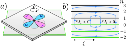
Figure 1: a) A Josephson junction made of two $d$–wave superconductors with a relative twist angle $\theta$. For $\theta=\pi/4$, the lowest-order Josephson coupling $J_{1}$ vanishes by symmetry. b) Cross section of the junction region. The layers of the two superconductors are labeled by $n$. The twist junction is between the $n=0$ and $n=1$ layers. The Josephson coupling between these layers is given by Eq. 1, and its spatial average vanishes at $\theta=\pi/4$. The Josephson coupling $\delta J_{1}(\bm{r})$ is correlated over a length $\xi$. The ground state breaks time reversal symmetry spontaneously, and is characterized by circulating persistent current loops, illustrated by blue arrows.

In this paper, we propose an alternative mechanism for the generation of $J_{2}$, a form of “order from disorder” driven by the effect of local spatial symmetry breaking. In Fig. 1a we schematically show a sample consisting of two $d$-wave superconductors rotated with respect to each other by an angle $\theta$. We consider the case where each superconductor contains $N$ layers, and we label them by the index $n$ which extends from $-N+1$ to $N$. We neglect the effect of inhomogeneity on all layers but those with $n=0,1$ (which are separated by the twist junction), and assume that the Josephson coupling per unit area between these layers has the form

$$J_{1}=\overline{J_{1}(\theta)}+\delta J_{1}({\bm{r}})$$ (1)

Here $\overline{J_{1}(\theta)}$ respects the $d$–wave symmetry so that it vanishes at $\theta=\pi/4$, while the random in sign quantity $\delta J_{1}$ is generated by a local, sample–specific point-group-symmetry breaking, such that $\overline{\delta J_{1}(\bm{r})}=0$. Here the overline denotes configuration averages over a random ensemble of $\delta J_{1}({\bf r})$.

The fluctuating component $\delta J_{1}(\bm{r})$ may arise from different physical sources. One possible source is spatial variations of the twist angle, $\delta\theta({\bm{r}})$, or any other form of disorder (including potential disorder) that breaks the local point group symmetries. A local admixture of an $s$–wave gap could also arise from “electron nematic domains.” We will comment on these possibilities further in the discussion section below.

We will characterise the fluctuations of $J_{1}$ by a correlation function

$$\overline{\delta J_{1}(\bm{r})\delta J_{1}(\bm{r}^{\prime})}=\overline{\delta J_{1}({\bm{r}})^{2}}\,f\left(\frac{|\bm{r}-\bm{r}^{\prime}|}{\xi}\right)$$ (2)

Here, $f(\bm{x})$ is a dimensionless function normalized such that $f(\bm{0})=1$ and $\int d^{2}xf(\bm{x})=1$, and $\xi$ is the correlation length of $\delta J_{1}(\bm{r})$.

The local inter-layer superconducting phase difference between the $n=0$ and $n=1$ layers, $\phi({\bm{r}})=\phi_{1}(\bm{r})-\phi_{0}(\bm{r})$, exhibits spatial fluctuations

$$\phi({\bm{r}})=\bar{\phi}+\delta\phi({\bm{r}})$$ (3)

which are correlated with the fluctuations of the critical current density $\delta J_{1}({\bm{r}})$. It is easy to show that at $\theta=\pi/4$ the ground state of the system corresponds to $\bar{\phi}=\pm\pi/2$. Indeed, for $\bar{\phi}=\pm\pi/2$, the system gains energy linearly in $\delta\phi$ by adjusting the phase difference across the junction to the sign of the local Josephson coupling $\delta J_{1}(\bm{r})$. The energy cost of the resulting in-plane currents is only quadratic in $\delta\phi$. This simple argument also implies the violation of the time-reversal symmetry, and existence of local circulating supercurrents and associated magnetic fields, illustrated in Fig. 1b. Time reversal symmetry is broken in an interval of twist angles near $\theta=\pi/4$.

Importantly, in the cuprates, the phase stiffness is strongly anisotropic, with the c-axis stiffness much smaller than the in-plane one. As a result, there is a characteristic length in the problem (treating, for simplicity, the case of $N=1$ – the case of $N\gg 1$ is discussed below)

$$\ell^{2}=\frac{\kappa}{(\overline{\delta J_{1}^{2}})^{1/2}},$$ (4)

where $\kappa$ is the in-plane phase stiffness. There are two regimes depending on $\xi/\ell$: In the case $\xi\gg\ell$ the system breaks into large domains with $\phi\approx 0$ or $\pi$, separated by by domain walls. Time reversal symmetry is broken in the vicinity of the domain walls where the phase twists from $0$ to $\pi$. In this case, the critical current through the junction is of the order of $(\overline{\delta J_{1}^{2}})^{1/2}$. Below we show that in the opposite limit, $\xi_{\text{sc}}\ll\xi\ll\ell$ (where $\xi_{\text{sc}}$ is the superconducting coherence length), the energy–phase relation has the form

$$E(\bar{\phi})=-\overline{J_{1}(\theta)}\cos(\bar{\phi})-J_{2}\cos(2\bar{\phi}),$$ (5)

where $J_{2}$ increases with $\xi$ (See Eqs. 13 below). For $\xi\sim\ell$, we obtain

$$|J_{2}|\sim|J_{2}^{\rm{max}}|\sim\sqrt{{\overline{\delta J_{1}^{2}}}}.$$ (6)

Thus, our mechanism is capable of producing a $J_{2}$ that is as large as the magnitude of the local (random) Josephson coupling, given that the correlation length of the local Josephson coupling is sufficiently large.

In the presence of an in-plane magnetic field $B_{\parallel}$, another length scale arises: $l_{B}=\Phi_{0}/(B_{\parallel}w)$, where $w$ is the smaller of the perpendicular penetration depth and the thickness of the device, and $\Phi_{0}$ is the superconducting flux quantum. As long as $l_{B}$ is larger than $\xi$, we expect the system to behave essentially as a Josephson junction with a spatially uniform $J_{1}$ and $J_{2}$. In particular, at $\theta=\pi/4$, the expected Fraunhofer pattern will reflect the doubled periodicity of the energy-phase relation. At higher fields (such that $l_{B}<\xi$) a more complicated interference pattern will directly reflect the inhomogeneity of the Josephson coupling [15].

Estimate of the intrinsic $J_{2}$.– As a first exercise, we estimate the intrinsic second-harmonic Josephson coupling $J_{2}$ generated by coherent tunneling of two Cooper pairs, neglecting the effects of inhomogeneity, and argue that the intrinsic $J_{2}$ is too small to account for the experiment of Ref. [7].

The measured values of the in-plane and out-of-plane penetration depths for optimally doped Bi-2212 are $\lambda_{\parallel}\sim 200$nm and $\lambda_{\perp}\sim 100\mu$m, respectively [16], corresponding to an anisotropic superfluid density, $\kappa_{\perp}/\kappa_{\parallel}=(\lambda_{\parallel}/\lambda_{\perp})^{2}\sim 4\times 10^{-6}$. This large anistropy reflects the extremely 2D electronic structure. To estimate the consequences of this for the expected ratio of $J_{2}/J_{1}$, we assume that the inter-layer tunneling is not momentum conserving (the “incoherent tunneling model” [17]), which reproduces the approximately $\cos(2\theta)$ dependence of $J_{1}$ observed in the experiments .

For $\theta\sim 0$, $J_{1}(0)$ (which has units of energy per unit area) is determined from an appropriate average of the inter-layer hopping, $t_{\perp}$, by an Ambagoakar-Baratoff-like relation

$$J_{1}(0)=g_{1}|t_{\perp}|^{2}\frac{\nu^{2}}{k_{F}^{2}}|\Delta|,$$ (7)

where $\nu$ is the density of states at the Fermi energy, $k_{F}$ is the Fermi wavevector, $|\Delta|$ is the size of the maximal gap, and $g_{1}$ is a dimensionless factor that depends, among other things, on the structure of the tunneling matrix elements in momentum space [18, 17]. Similar reasoning gives for the intrinsic second order coupling

$$J_{2}=g_{2}|t_{\perp}|^{4}\frac{\nu^{3}}{k_{F}^{4}},$$ (8)

where $g_{2}$ is another dimensionless factor, and presumably $J_{2}$ is approximately independent of $\theta$.

To relate these $J_{1}$ and $J_{2}$ to measured quantities, we assume that the coupling between planes in a bulk crystal is the same as for the twist junction with $\theta\sim 0$, so that we can identify $\kappa_{\perp}=J_{1}(0)d$, where $d$ is the inter-bilayer distance. (For further consistency checks regarding the estimate of $J_{1}$ and $J_{2}$, see Supplementary Information.) Moreover, the in-plane superfluid stiffness empirically satisfies $\kappa_{\parallel}=g_{\parallel}T_{c}/d$ where $g_{\parallel}$ is of order one. Therefore

$$\left(\frac{J_{2}}{J_{1}(0)}\right)=\left(\frac{g_{\parallel}g_{2}}{g_{1}^{2}}\right)\left(\frac{\xi_{\text{sc}}}{k_{F}d^{2}}\right)\left(\frac{T_{c}}{\left|\Delta\right|}\right)\left(\frac{\kappa_{\perp}}{\kappa_{\parallel}}\right).$$ (9)

Taking into account the fact that in optimally doped cuprates $T_{c}$ and $|\Delta|$ are of the same order of magnitude, and so are $1/k_{F}$, $d$, and $\xi_{\text{sc}}$, and ignoring the unknown numerical prefactors, we get that the intrinsic value of $J_{2}/J_{1}$ should be of the order of $10^{-6}-10^{-5}$. In contrast, the measured value of $J_{2}/J_{1}$ reported in Ref. [7] is $\sim 10^{-2}$. Thus, unless for some reason $g_{1}$ is anomalously small, or $g_{2}$ unexpectedly large, the intrinsic effect is too small to account for the cuprate experiment.

Inhomogeniety–induced $J_{2}$.– We use the following model to describe two layered superconductors coupled by a twisted Josephson junction:

$$\mathcal{H}=\sum_{n}\int d^{2}r\,\Big{[}\frac{\kappa}{2}\left(\nabla\phi_{n}\right)^{2}-\mathcal{J}^{(n)}\cos\left(\phi_{n}-\phi_{n-1}\right)\Big{]},$$ (10)

where $\phi_{n}(\bm{r})$ is the superconducting phase in layer $n$ at position $\bm{r}=(x,y)$, and $\kappa=\kappa_{\parallel}d$ is the phase stiffness in the plane. Each superconductor contains $N$ layers, and the sum over $n$ extends from $-N+1$ to $N$. For $n\neq 1$, the inter-plane coupling per unit area is $\mathcal{J}^{(n)}=J_{1}(0)$, related to the three-dimensional phase stiffness by $J_{1}(0)=\kappa_{\perp}/d\equiv J_{\perp}$. For $n=1$, the Josephson coupling is $\mathcal{J}^{(1)}=J_{1}(\bm{r})$, given by Eq. 1.

Note that we ignore magnetic screening throughout the analysis, neglecting the coupling of the superconducting phase to the electromagnetic field. This assumption is justified as long as the thickness of the system is much smaller than $\lambda_{\perp}$, and the lateral size is smaller than the Josephson penetration depth of the twist junction.

We analyze the system at $T=0$, minimizing the energy (10). A similar analysis was performed in 3D case in Ref. [19]; here, we generalize the analysis for the case of layered superconductors and a finite correlation length of the local Josephson coupling $\delta J_{1}(\bm{r})$.

For $\xi\ll\ell$ (where $\ell$ is defined in Eq. 4 for $N=1$ and in Eq. 14 below for $N\rightarrow\infty$), the superconducting phase is nearly uniform within each of the two superconductors. We therefore write the superconducting phase as $\phi_{n}(\bm{r})=s_{n}\bar{\phi}/2+\delta\phi_{n}(\bm{r})$, where $s_{n}=1$ for $n>0$ and $-1$ otherwise ($\bar{\phi}$ is the average phase difference), and expand the energy up to second order in $\delta\phi_{n}(\bm{r})$. Minimizing the resulting expression, we obtain the energy-phase relation of the junction per unit area given by Eq. 5 with the second-order Josephson coupling is given by

$$J_{2}=-\int\frac{d^{2}q}{(2\pi)^{2}}\frac{\left|\delta J_{1}(\bm{q})\right|^{2}}{\kappa q^{2}+J_{\perp}\frac{1-e^{-\eta_{\bm{q}}}+\alpha_{\bm{q}}\left(1-e^{\eta_{\bm{q}}}\right)}{1+\alpha_{\bm{q}}}}.$$ (11)

(See Supplementary Information for further details.) Here, $\delta J_{1}(\bm{q})$ is the Fourier transform of $\delta J_{1}(\bm{r})$, $\eta_{\bm{q}}=\cosh^{-1}[1+\kappa q^{2}/(2J_{\perp})]$, and

$$\alpha_{\bm{q}}=e^{-2\eta_{\bm{q}}\left(N-1\right)}\frac{J_{\perp}\left(e^{\eta_{\bm{q}}}-1\right)-\kappa q^{2}}{J_{\perp}\left(1-e^{-\eta_{\bm{q}}}\right)+\kappa q^{2}}.$$ (12)

Crucially, the sign of $J_{2}$ is negative. Therefore, at twist angle $\theta=\pi/4$ [such that $J_{1}(\theta)=0$], the ground state corresponds to $\phi=\pm\pi/2$. Time reversal symmetry is broken in a range of twist angles around $\pi/4$, such that $|J_{2}|>|J_{1}(\theta)|/4$. We provide explicit expressions for $J_{2}$ in two cases:

$$J_{2}\approx-\frac{\overline{\delta J_{1}^{2}}\xi^{2}}{2\pi\kappa}\begin{cases}\ln\left(1+\frac{1}{\xi}\sqrt{\frac{\kappa}{J_{1}(0)}}\right),&N\rightarrow\infty,\\ \ln\left(\frac{\kappa}{\left(\overline{\delta J^{2}}\right)^{1/2}\xi^{2}}\right),&N=1.\end{cases}$$ (13)

The expressions are valid if $\xi$ is sufficiently short: $\xi\ll\ell$, such that $\delta\phi_{n}(\bm{r})\ll\pi$. Beyond this regime ($\xi>\ell$), the perturbative calculation breaks down (see discussion around Eq. 4). The length scale $\ell$ can be identified as the value of $\xi$ where $J_{2}\sim(\overline{\delta J^{2}_{1}})^{1/2}$. Using Eq. 13, this gives Eq. 4 for $N=1$ (up to the logarithmic factor, which is of the order of unity in this case), whereas for $N\rightarrow\infty$ we find

$$\ell^{2}\sim\frac{\kappa J_{1}(0)}{\overline{\delta J_{1}^{2}}}.$$ (14)

For $N=1$, the derivation of Eq. 13 contains a subtlety - the integral in Eq. 11 is infrared divergent. This logarithmic divergence occurs also for any finite $N$, and signals a breakdown of the perturbative treatment in $\delta J_{1}$. A more accurate treatment (see Supplementary Information) reveals that the divergence is cut off by an emergent length scale, of the order of $\ell^{2}/\xi$, which leads to Eq. 13.

Importantly, comparing Eq. 13 to Eq. 9, we find that the inhomogeneity-induced $J_{2}$ differs from the intrinsic one by a factor of

$$\frac{J_{2}}{J^{\text{int}}_{2}}\sim\frac{\overline{\delta J_{1}^{2}}}{J_{1}^{2}(0)}\left(\frac{\xi}{\xi_{\text{sc}}}\right)^{2},$$ (15)

where we have dropped all factors of order one.

Discussion.– The vanishing of $J_{1}(\theta)$ as $\theta\to\pi/4$ and the existence of a higher order Josephson coupling, $J_{2}$ that is non-vanishing under the same conditions follow from the $d-$wave symmetry of the SC order. There are, generically, both intrinsic and extrinsic (disorder related) contributions to $J_{2}(\theta)$. However, given the extremely small c-axis superfluid density in the particular material of interest (Bi-2212), the observed [7] magnitude, $|J_{2}(\pi/4)/J_{1}(0)|\sim 10^{-2}$ is notably large. We have estimated that the intrinsic contribution is of order $|J_{2}^{\text{int}}(\pi/4)/J_{1}(0)|\sim 10^{-5}-10^{-6}$ (Eq. 9). What we have shown is that an extrinsic mechanism - one that derives from a fluctuating in space but random in sign first order coupling $J_{1}(\bm{r})$ - can produce an effect of the requisite magnitude but only under rather extreme circumstances, i.e. when $\overline{\delta J_{1}^{2}}/J_{1}^{2}(0)$ is sufficiently large and the correlation length, $\xi$, is relatively long. For instance, we can explain the observed value of $|J_{2}/J_{1}(0)|$ if we assume $\overline{\delta J_{1}^{2}}/J_{1}^{2}(0)=0.1$ and $\xi/\xi_{\text{sc}}\sim 10^{2}-10^{3}$.

The existence of a non-vanishing $\delta J_{1}(\bm{r})$ when globally $\theta=\pi/4$ requires a local breaking of mirror symmetries (where the mirror plane is perpendicular to the system). Twist-angle disorder leads to such symmetry breaking. However, to produce an effect of the requisite magnitude observed in Ref. [7], either the distribution of the twist angles should be a substantial fraction of $\pi/4$, or their correlation length should be larger than the sample size (about 10$\mu$m). Some source of substantial shear-strain disorder might also be relevant, but there would need to be some reason to believe that such strain would strongly perturb the local pairing symmetry.

We thus consider the most likely origin of the requisite disorder is to be pinned domains of an otherwise intrinsic electron-nematic order [20]. There exists strong - although not universally accepted - evidence of a tendency toward nematic order in the cuprates [21, 22, 23, 24, 25]. In particular, in Bi-2212, there is direct evidence from scanning tunnelling microscopy (STM) [24, 26, 27, 28, 29] of local nematic order which is seen strongly and primarily at energies of order of the gap maximum (i.e. at energies at which the density of states in the superconducting state exhibits a maximum). This implies that the local nematicity has a strong effect on the local superconducting order parameter. Moreover, the fact that signatures of nematic symmetry breaking remain strong when STM features are spatially averaged over the field of view suggests a correlation length larger than the field of view, i.e. $\xi_{\text{nem}}>100a$ (where $a$ is the lattice spacing). In addition, a recent STM study [28] on a related material (Bi-2201) also provides evidence of long-range nematic correlations.[30]

There are several testable consequences of various aspects of the above line of reasoning: 1) An extrinsic effect depends strongly on $\xi$ and $\overline{\delta J_{1}^{2}}$, which could well depend on details of sample preparation. This, in turn, might explain the already mentioned fact that the twist-angle dependence is not universally observed [8]. 2) The time reversal breaking phase should have spontaneous circulating currents, as shown in Fig. 1b. The expected order of magnitude of the in-plane magnetic moment is $m_{\parallel}\sim(2e/\hbar)\,(\overline{\delta J^{2}_{1}})^{1/2}\xi^{3}d$. Taking $\overline{(\delta J^{2}_{1}})^{1/2}\sim 0.3\,J_{1}(0)\sim 1.5\cdot 10^{-5}\rm{meV}/\rm{nm}^{2}$, $\xi=200\rm{nm}$ and $d=1.5\rm{nm}$, this gives $m_{\parallel}$ of the order of a few $\mu_{B}$. The associated magnetic fields should be observable near the edges of the system, and have a random sign. 3) From STM [26] and other [31] studies, it appears that the nematicity in Bi-2212 vanishes (or at least becomes much weaker) for hole doping concentration larger than a critical value, $p^{\star}\approx 0.19$. Thus, a correspondingly strong doping dependence of the magnitude of $J_{2}$ would be expected if electron-nematicity plays a role in the effect.[32]

From a symmetry point of view, the state of the system at $\theta=\pi/4$ is, as has been previously noted [9], a $d+id$ superconductor. In the absence of disorder (assuming that $J_{2}$ is generated by the intrinsic mechanism), this state should be fully gapped - although for numbers relevant to Bi-2212 this induced nodal gap $\Delta_{\text{ind}}$ would likely be immeasurably small. For the extrinsic case, there is an interesting question of principle whether this state is gapped or gapless. Potential disorder is expected to suppress the gap. The gap is further reduced by local Doppler shifts of the quasi-particle energies (Volovik effect [33]) due to the presence of equilibrium currents, $\delta E(\bm{r})=v_{F}j_{s}(\bm{r})/\kappa$. If this energy shift is larger than $\Delta_{\text{ind}}(\bm{r})$, the gap closes.

Finally, we note that the present considerations are not confined to the cuprates. In less anisotropic systems, there may be circumstances in which the intrinsic effect dominates, and in which the resulting state at $\theta=\pi/4$ is fully gapped, as suggested in Ref. [9]. It is also worth noting that very similar considerations apply to a junction between an unconventional superconductor (e.g. a d-wave superconductor) and a conventional s-wave superconductor, without need for twist angle engineering.

I Acknowledgments

We are grateful to J. C. Davis, P. Kim, M. Franz, and A. Pasupathy, J. Pixley, and J. M. Tranquada for useful discussions. We thank the hospitality of the Aspen Center for Physics and the Oxford Physics Department, where part of this work was done. SAK and AY were supported, in part, by NSF grant No. DMR-2000987 at Stanford and SAK was further supported by a Leverhulme Trust International Professorship grant numberLIP-202-014 at Oxford. The work BZS was funded by the Gordon and Betty Moore Foundation’s EPiQS Initiative through Grant GBMF8686. YV and EB were supported by the European Research Council (ERC) under the European Union’s Horizon 2020 research and innovation programme (grant agreement No 817799) and by the Israel-USA Binational Science Foundation (BSF).

Appendix A Further Quantitative Considerations

The most crucial parameter for quantitative estimates of $J_{1}$ and $J_{2}$ is the inter-bilayer tunneling matrix element, $t_{\perp}$. Estimates of this parameter from band structure calculations vary from a few meV [34] to as much as $20$meV [9]. Moreover, $t_{\perp}$ may have a significant angle dependence [14]. The largest of these estimates could give rise intrinsic values of $J_{2}/J_{1}$ that are compatible with the experiment of Ref. [7].

Considering the significant variation of the first principle estimates, and the fact that $t_{\perp}$ could exhibit a large many-body renormalization [35], we take a more empirical approach. Several measurable quantities are expected to be proportional to $t_{\perp}^{2}$: these include $\kappa_{\perp}$, the bulk c-axis critical current density $J_{c}$, the bulk c-axis conductivity, the critical current of the junction at $\theta=0$, and the inverse of the normal state junction resistance $R^{-1}_{N}$. As we enumerate below, these various quantities all give a roughly consistent estimate, $(t_{\perp}/t)^{2}\sim 10^{-5}$ (where $t$ is the in-plane hopping matrix element). Taking $t\approx 0.25$eV, this gives $t_{\perp}\sim 1$meV, and the estimates of $J_{2}/J_{1}(0)$ quoted in the main text.

As was noted in Ref. [7], the $\theta=0$ critical current density of the junction is similar to the bulk $c-$axis critical current density of optimally doped Bi-2212. This confirms that the coupling across the junction is of similar magnitude to the inter-bilayer bulk coupling. The c-axis phase stiffness inferred from the critical currents reported in Refs. [7, 36], $J_{c}\approx 1\rm{kA}/\rm{cm}^{2}$, given by

$$\kappa_{\perp}=\frac{\hbar J_{c}d}{2e}\approx 3.1\cdot 10^{-5}\rm{meV/nm},$$ (16)

is consistent within a factor of 2 with the estimate of $\kappa_{\perp}$ from the c-axis penetration depth, using $\lambda_{c}=100\mu$m [16],

$$\kappa_{\perp}=\frac{1}{\mu_{0}(2e/\hbar)^{2}}\,\frac{1}{\lambda_{c}^{2}}\approx 5.4\cdot 10^{-5}\rm{meV/nm}.$$ (17)

As noted in the text, these values point to a ratio $\kappa_{\perp}/\kappa_{\parallel}\approx 4\cdot 10^{-6}$. The resistivity anisotropy of optimally doped Bi-2212 at $T=T_{c}$ is $\rho_{ab}/\rho_{c}\approx 10^{-5}$ [37], and the anisotropy tends to increase with decreasing temperature.

A further consistency check is provided by the Ambegaokar-Baratoff relation [38]. In Ref. [7], the values of the normal state junction resistance $R_{N}$ and the critical current $I_{c}$ are reported for various samples with different twist angles. For those with $\theta$ near $0$, The product $I_{c}R_{N}$ is about $15$meV, which is smaller than (but of the order of) $\pi\Delta_{\rm{max}}/(2e)$, where $\Delta_{\rm{max}}\approx 40$meV is the maximal gap inferred from various spectroscopy experiments [39]. This indicates that near $\theta=0$, the critical current is not dramatically suppressed due to destructive interference (as may arise, e.g., in a dirty junction between $d$-wave superconductors). Near $\theta=\pi/4$, $I_{c}R_{N}$ is smaller by a factor of about $50$, similar to the suppression of $I_{c}$.

Appendix B Perturbation Theory

Here, we provide more details on the perturbative treatment of the Hamiltonian in Eq. 10. We use the following ansatz for $\phi_{n}(\bm{r})$:

$$\phi_{n}(\bm{r})=\begin{cases}\,\,\,\frac{\bar{\phi}}{2}+\varphi_{n}(\bm{r}),&n>0,\\ -\frac{\bar{\phi}}{2}-\varphi_{-n+1}(\bm{r}),&n\leq 0.\end{cases}$$ (18)

We insert Eq. 18 into Eq. 10, minimize with respect to $\varphi_{n}({\bm{r}})$ and linearize the resulting equations. This gives:

$$-\kappa\nabla^{2}\varphi_{n}+J_{\perp}\left(2\varphi_{n}-\varphi_{n+1}-\varphi_{n-1}\right)=0\,\,\,(1<n<N),$$ (19)

$$-\kappa\nabla^{2}\varphi_{1}+J_{\perp}\left(\varphi_{1}-\varphi_{2}\right)+J_{1}(\bm{r})\sin\bar{\phi}=0,$$ (20)

$$-\kappa\nabla^{2}\varphi_{N}+J_{\perp}\left(\varphi_{N}-\varphi_{N-1}\right)=0.$$ (21)

We insert a solution of the form

$$\varphi_{n}(\bm{r})=\sum_{\bm{q}}e^{i\bm{q}\cdot\bm{r}}\left(A_{\bm{q}}e^{\eta_{\bm{q}}\left(n-1\right)}+B_{\bm{q}}e^{-\eta_{\bm{q}}\left(n-1\right)}\right)\,\,\,(n>0),$$ (22)

and $\varphi_{-n}(\bm{r})=-\varphi_{n+1}(\bm{r})$.

From Eq. (19),

$$\kappa q^{2}+2J_{\perp}\left(1-\cosh\eta_{\bm{q}}\right)=0,$$ (23)

i.e.

$$\eta_{\bm{q}}=\cosh^{-1}\left(1+\frac{\kappa q^{2}}{2J_{\perp}}\right)=\ln\left[\left(1+\frac{\kappa q^{2}}{2J_{\perp}}\right)+\sqrt{\left(1+\frac{\kappa q^{2}}{2J_{\perp}}\right)^{2}-1}\right].$$ (24)

The two useful limits of this expression are

$$\eta_{\bm{q}}\rightarrow\sqrt{\frac{\kappa}{J_{\perp}}}q,\,\,\,q\ll\sqrt{\frac{J_{\perp}}{\kappa}},$$ (25)

$$\eta_{\bm{q}}\rightarrow\ln\left(\frac{\kappa q^{2}}{J_{\perp}}\right),\,\,\,q\gg\sqrt{\frac{J_{\perp}}{\kappa}}.$$ (26)

To solve for $A_{\bm{q}}$ and $B_{\bm{q}}$, we use Eq. (21), obtaining

$$A_{\bm{q}}=B_{\bm{q}}\alpha_{\bm{q}},$$ (27)

where

$$\alpha_{\bm{q}}=e^{-2\eta_{\bm{q}}\left(N-1\right)}\frac{J_{\perp}\left(e^{\eta_{\bm{q}}}-1\right)-\kappa q^{2}}{J_{\perp}\left(1-e^{-\eta_{\bm{q}}}\right)+\kappa q^{2}}.$$ (28)

Note that, in the limit $q\rightarrow 0$, $\alpha_{q}\rightarrow 1$, and that $\alpha_{\bm{q}}>0$ (this is shown using Eq. 24). For later use, we note also that (for $N>1$)

$$\alpha_{\bm{q}} =e^{-2\eta_{\bm{q}}\left(N-1\right)}\frac{J_{\perp}\left(e^{\eta_{\bm{q}}}-1\right)-\kappa q^{2}}{J_{\perp}\left(1-e^{-\eta_{\bm{q}}}\right)+\kappa q^{2}}\leq e^{-2\eta_{\bm{q}}\left(N-1\right)}\frac{J_{\perp}\left(e^{\eta_{\bm{q}}}-1\right)}{J_{\perp}\left(1-e^{-\eta_{\bm{q}}}\right)}$$

$$=e^{-2\eta_{\bm{q}}\left(N-1\right)}e^{\eta_{\bm{q}}}\leq e^{-\eta_{\bm{q}}}.$$ (29)

Using Eq. (20), we find

$$B_{\bm{q}}=-\frac{J_{1}(\bm{q})\sin\bar{\phi}}{\kappa q^{2}\left(1+\alpha_{\bm{q}}\right)+J_{\perp}\left(1-e^{-\eta_{\bm{q}}}+\alpha_{\bm{q}}\left(1-e^{\eta_{\bm{q}}}\right)\right)},$$ (30)

and hence

$$\varphi_{1}(\bm{r})=\frac{1}{A}\sum_{\bm{q}}e^{i\bm{q}\cdot\bm{r}}\frac{J_{1}(\bm{q})\sin\bar{\phi}\left(1+\alpha_{\bm{q}}\right)}{\kappa q^{2}\left(1+\alpha_{\bm{q}}\right)+J_{\perp}\left(1-e^{-\eta_{\bm{q}}}+\alpha_{\bm{q}}\left(1-e^{\eta_{\bm{q}}}\right)\right)}.$$ (31)

At $\theta=\pi/4$ (such that $\overline{J_{1}}=0$), the current-phase relation of the junction is given by:

$$I(\bar{\phi}) =\sum_{\bm{q}}2\cos(\bar{\phi})J_{1}(\bm{q})\varphi(-\bm{q})=-\sum_{\bm{q}}\frac{\left|J_{1}(\bm{q})\right|^{2}\left(1+\alpha_{\bm{q}}\right)\sin 2\bar{\phi}}{\kappa q^{2}\left(1+\alpha_{\bm{q}}\right)+J_{\perp}\left(1-e^{-\eta_{\bm{q}}}+\alpha_{\bm{q}}\left(1-e^{\eta_{\bm{q}}}\right)\right)}$$

$$=-\sum_{\bm{q}}\frac{\left|J_{1}(\bm{q})\right|^{2}}{\kappa q^{2}+J_{\perp}\frac{1-e^{-\eta_{\bm{q}}}+\alpha_{\bm{q}}\left(1-e^{\eta_{\bm{q}}}\right)}{1+\alpha_{\bm{q}}}}\sin 2\bar{\phi},$$ (32)

which gives Eq. 11 in the main text. Note that the denominator is non-negative:

$$\frac{1-e^{-\eta_{\bm{q}}}+\alpha_{\bm{q}}\left(1-e^{\eta_{\bm{q}}}\right)}{1+\alpha_{\bm{q}}}=\left(1-e^{-\eta_{\bm{q}}}\right)\frac{1-\alpha_{\bm{q}}e^{\eta_{\bm{q}}}}{1+\alpha_{\bm{q}}}\geq 0,$$ (33)

where we have used Eq. (29).

Appendix C Self-consistent treatment

We consider the Hamiltonian of Eq. 10 for the case $N=1$ (one layer in each side of the junction) and $\theta=\pi/4$ (i.e., $\overline{J_{1}}=0$). The Hamiltonian for the relative phase $\varphi(\bm{r})=\phi_{1}(\bm{r})-\phi_{0}(\bm{r})$ is written as:

$$H=\int d^{2}r\left[\frac{\kappa}{2}\left(\nabla\varphi\right)^{2}-\delta J_{1}(\bm{r})\cos[\varphi(\bm{r})])\right],$$ (34)

We now discuss the infra-red divergence encountered in the perturbative treatment, and how it can be cured by performing a self-consistent harmonic calculation. The latter analysis reveals an emergent length scale which appears in the logarithm in Eq. 13 for $N=1$. A similar divergence appears, and can be treated in a similar fashion, for any finite $N$.

The perturbative expression for the phase in the first layer is given by Eq. 31 with $J_{\perp}=0$ and $\alpha_{q}=0$. Then, we find that the variance of $\varphi_{1}(\bm{r})$ is

$$\overline{\varphi^{2}(\bm{r})}=\int\frac{d^{2}q}{(2\pi)^{2}}\frac{\overline{\delta J_{1}(\bm{q})\delta J_{1}(\bm{-q})}}{\left(\kappa q^{2}\right)^{2}}.$$ (35)

This is infrared divergent, signalling a breakdown of the perturbative treatment at long wavelengths. To deal with this divergence, we perform a self-consistent harmonic approximation. Writing $\varphi(\bm{r})=\pi/2-\varphi_{v}(\bm{r})$, we replace Eq. 34 with a variational Hamiltonian:

$$H_{var}=\int d^{2}r\left[\frac{\kappa}{2}\left(\nabla\varphi_{v}\right)^{2}+\frac{m^{2}}{2}\varphi_{v}^{2}-\delta J_{1}(\bm{r})\varphi_{v}(\bm{r})\right],$$ (36)

and minimize $H[\varphi_{v}(\bm{r})]$ with respect to $m$, with $\varphi_{v}(\bm{r})$ taken to be the minimizer of $H_{var}$:

$$\varphi_{v}(\bm{q})=\frac{\delta J_{1}(\bm{q})}{\kappa q^{2}+m^{2}}$$ (37)

In real space,

$$\varphi_{v}(\bm{r})=\int d^{2}r^{\prime}K(\bm{r}-\bm{r}^{\prime})\delta J_{1}(\bm{r}^{\prime}),\quad K(\bm{r})=\frac{1}{A}\sum_{\bm{q}}\frac{1}{\kappa q^{2}+m^{2}}e^{i\bm{q}\cdot\bm{r}}.$$ (38)

The variational energy is given by:

$$\overline{H[\varphi_{v}(\bm{r})]}=A\sum_{\bm{q}}\frac{\kappa q^{2}\,\overline{\delta J_{1}(\bm{q})\delta J_{1}(\bm{-q})}}{2\left(\kappa q^{2}+m^{2}\right)^{2}}-\int d^{2}r\,\overline{\delta J_{1}(\bm{r})\sin\varphi_{v}(\bm{r})},$$ (39)

where

$$\int d^{2}r\,\overline{\delta J_{1}(\bm{r})\sin\varphi_{v}(\bm{r})} =\frac{1}{2i}\int d^{2}r\,\overline{\delta J_{1}(\bm{r})e^{i\varphi_{v}(\bm{r})}}+c.c.$$

$$=\frac{1}{2i}\int d^{2}r\overline{\delta J_{1}(\bm{r})e^{i\int d^{2}r^{\prime}K(\bm{r}-\bm{r}^{\prime})\delta J_{1}(\bm{r}^{\prime})}}+c.c.$$

$$=\frac{1}{2i}\int d^{2}r\left(\frac{1}{i}\frac{\delta}{\delta\alpha(\bm{r})}\right)\overline{e^{i\int d^{2}r^{\prime}\left[K(\bm{r}-\bm{r}^{\prime})+\alpha(\bm{r}^{\prime}))\right]\delta J_{1}(\bm{r}^{\prime})}}\Big{|}_{\alpha=0}+c.c.$$

$$=\frac{1}{2i}\int d^{2}r\left(\frac{1}{i}\frac{\delta}{\delta\alpha(\bm{r})}\right)e^{-\frac{1}{2}\int d^{2}r^{\prime\prime}\int d^{2}r^{\prime}\left[K(\bm{r}-\bm{r}^{\prime})+\alpha(\bm{r}^{\prime})\right]\left[K(\bm{r}-\bm{r}^{\prime\prime})+\alpha(\bm{r}^{\prime\prime})\right]\overline{\delta J_{1}(\bm{r}^{\prime})\delta J_{1}(\bm{r}^{\prime\prime})}}|_{\alpha=0}+c.c.$$

$$=\sum_{\bm{q}}\frac{\overline{\delta J_{1}(\bm{q})\delta J_{1}(-\bm{q})}}{\kappa q^{2}+m^{2}}\exp\left[-\frac{1}{A}\sum_{\bm{q}}\frac{\overline{\delta J_{1}(\bm{q})\delta J_{1}(-\bm{q})}}{\left(\kappa q^{2}+m^{2}\right)^{2}}\right],$$ (40)

where we have taken the distribution of $J_{1}(\bm{r})$ to be Gaussian. We assume that $\xi\ll\sqrt{\kappa}/m$ (we will check the validity of this assumption below). Then, $\overline{\delta J_{1}(\bm{q})\delta J_{1}(-\bm{q})}$ can be replaced by $\overline{\delta J_{1}(\bm{q}=0)^{2}}=A\overline{\delta J_{1}(\bm{r})^{2}}\xi^{2}$, and the upper cutoff of the momentum integrals is given by $1/\xi$. Evaluating the integrals, we obtain the variational energy

$$E(m^{2})=\overline{H[\varphi_{v}]}=Am_{0}^{2}\left[\frac{1}{2}\left(\ln\frac{\kappa}{m^{2}\xi^{2}}-1\right)-\ln\frac{\kappa}{m^{2}\xi^{2}}e^{-\frac{m_{0}^{2}}{2m^{2}}}\right],$$ (41)

where we have defined

$$m_{0}^{2}=\frac{\overline{\delta J_{1}^{2}}\xi^{2}}{4\pi\kappa}=\frac{\kappa}{4\pi\ell^{2}}\frac{\xi^{2}}{\ell^{2}},\quad\ell^{2}=\frac{\kappa}{(\overline{\delta J_{1}^{2}})^{1/2}}$$ (42)

Where $\ell$ is the disorder length scale for $N=1$ as discussed in Eq. 4. Minimizing the energy:

$$\frac{\partial}{\partial m^{2}}E(m^{2})=A\frac{m_{0}^{2}}{2m^{2}}\left[-\frac{1}{2}+\left(1-\frac{m_{0}^{2}}{2m^{2}}\ln\frac{\kappa}{m^{2}\xi^{2}}\right)e^{-\frac{m_{0}^{2}}{2m^{2}}}\right]=0,$$ (43)

We assume that $\frac{m_{0}^{2}}{2m^{2}}\ll 1$, to be checked self-consistently. Then, the exponent $e^{-\frac{m_{0}^{2}}{2m^{2}}}\approx 1$ to leading order in $\frac{m_{0}^{2}}{2m^{2}}$, and we obtain

$$\frac{m_{0}^{2}}{2m^{2}}\ln\frac{\kappa}{m^{2}\xi^{2}}\approx\frac{1}{2}.$$ (44)

The solution, to leading order in logs, is

$$m^{2}\approx m_{0}^{2}\ln\frac{\kappa}{m_{0}^{2}\xi^{2}}=\frac{\overline{\delta J_{1}^{2}}\xi^{2}}{4\pi\kappa}\ln\frac{4\pi\kappa^{2}}{\overline{\delta J_{1}^{2}}\xi^{4}}=\frac{\kappa}{4\pi\ell^{2}}\frac{\xi^{2}}{\ell^{2}}\ln\frac{4\pi\ell^{4}}{\xi^{4}}$$ (45)

Our calculation is valid if $\xi\ll\ell$. Under this condition, the assumption

$$\frac{m_{0}^{2}}{2m^{2}}=\frac{1}{2}\left(\ln\frac{4\pi\ell^{4}}{\xi^{4}}\right)^{-1}\ll 1$$ (46)

used above is justified. Furthermore, substituting $m$ into the minimizer $\varphi_{v}$, we find that

$$\overline{\varphi_{v}(\bm{r})^{2}}\propto\frac{m_{0}^{2}}{m^{2}}\ll 1$$ (47)

Where $\propto$ denotes a possible constant of order 1. As mentioned in the main text, in the opposite limit ($\xi\gg\ell$), the system breaks into domains where $\varphi$ is close to either $0$ or $\pi$; this regime is not captured in the self-consistent harmonic treatment.

In summary, we find that in the two-dimensional case and for sufficiently small $\xi$, the fluctuations of the phase difference across the junction are correlated over the emergent length scale $\sqrt{\kappa}/m\gg\ell\gg\xi$, where $\sqrt{\kappa}/m$ is given by Eq. 45 and rewritten as follows.

$$\frac{\sqrt{\kappa}}{m}=\frac{4\pi\ell^{2}}{\xi}\left(\ln\frac{4\pi\ell^{4}}{\xi^{4}}\right)^{-1/2}$$ (48)

If $\xi$ exceeds $\sqrt{\kappa}/m\gg\ell$, the system breaks into domains where the phase is locked to either $0$ or $\pi$.

Appendix D Numerics

We can test the analysis outlined in Appendices B and C by minimizing the energy numerically for a large system for different values of $\delta J$. To this end, we use a lattice version of problem, with a Hamiltonian

$$H_{latt}=-\kappa\sum_{n=0,1,\langle ij\rangle}\cos(\phi_{i,n}-\phi_{j,n})-\sum_{i}\delta J_{i}\cos(\phi_{i,1}-\phi_{i,0}).$$ (49)

Here, $\phi_{i,n}$ is the superconducting phase of lattice site $i$ and layer $n=0,1$, $\langle ij\rangle$ denotes a pair of nearest-neighbor sites $i$ and $j$, and $\delta J_{i}$ is the inter-plane coupling, taken for simplicity to be uniformly distributed in the range $[-\delta J,\delta J]$. Physically, the lattice spacing corresponds to the length scale $\xi$, over which $J_{1}(\bm{r})$ is correlated.

As expected, the ground state is found to break time reversal symmetry, with the average phase difference $\phi_{i,1}-\phi_{i,0}$ close to either $-\pi/2$ or $\pi/2$. Which of the two states is selected is determined by the initial conditions of the minimization. Choosing the state with $\overline{\phi_{i,1}-\phi_{i,0}}\approx\pi/2$, We define $\varphi_{i}=\phi_{i,1}-\phi_{i,0}-\pi/2$, and examine the correlation function

$$C(\bm{q})=\overline{\varphi_{\bm{q}}\varphi_{-\bm{q}}},$$ (50)

where $\varphi(\bm{q})=\sum_{j}e^{-i\bm{q}\cdot\bm{r_{j}}}\varphi_{j}$. The data is fit to the form

$$C(q,m)=\frac{C_{0}}{\left(q^{2}+m^{2}\right)^{2}},$$ (51)

anticipated from the self-consistent harmonic approximation.

The calculated $C(q)$ (solid lines) and the fits (dashed lines) are shown in the left panel of Fig. 2 for different values of $\delta J/\kappa$. The system size is $800\times 800$, and the $C(q)$ was averaged over 8 disorder realization. We have checked that there are no significant finite size effects, even for the smallest value of $\delta J$. We find that $C_{0}\propto\delta J^{2}$. The right hand panel shows the fitting parameter $m$ as a function of $\delta J$. the solid line is a fit to Eq. (45), of the form:

$$m(\delta J)=m_{1}\delta J\sqrt{\ln\frac{m_{2}}{\delta J}},$$ (52)

where $m_{1}$ and $m_{2}$ are fitting parameters.

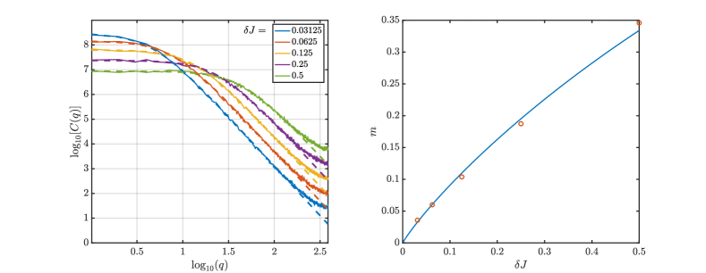
Figure 2: Numerical results. Left: log-log plot of the correlation function $C(q,\delta J)=\overline{\varphi_{q}\varphi_{-q}}$. The dashed lines are fits to Eq. 51. Note that at large $q$, $C(q)\sim q^{-4}$, whereas at small $q$, $C(q)\rightarrow const.$ We use units such that $\kappa=1$. Right: the inverse correlation length $m$ from the fits, as a function of $\delta J$. The solid line is a fit to Eq. 52.

References

- Cao et al. [2018a] Y. Cao, V. Fatemi, A. Demir, S. Fang, S. L. Tomarken, J. Y. Luo, J. D. Sanchez-Yamagishi, K. Watanabe, T. Taniguchi, E. Kaxiras, et al., Correlated insulator behaviour at half-filling in magic-angle graphene superlattices, Nature 556, 80 (2018a).
- Cao et al. [2018b] Y. Cao, V. Fatemi, S. Fang, K. Watanabe, T. Taniguchi, E. Kaxiras, and P. Jarillo-Herrero, Unconventional superconductivity in magic-angle graphene superlattices, Nature 556, 43 (2018b).
- Yankowitz et al. [2019] M. Yankowitz, S. Chen, H. Polshyn, Y. Zhang, K. Watanabe, T. Taniguchi, D. Graf, A. F. Young, and C. R. Dean, Tuning superconductivity in twisted bilayer graphene, Science 363, 1059 (2019).
- Polshyn et al. [2019] H. Polshyn, M. Yankowitz, S. Chen, Y. Zhang, K. Watanabe, T. Taniguchi, C. R. Dean, and A. F. Young, Large linear-in-temperature resistivity in twisted bilayer graphene, Nature Physics 15, 1011 (2019).
- Inbar et al. [2023] A. Inbar, J. Birkbeck, J. Xiao, T. Taniguchi, K. Watanabe, B. Yan, Y. Oreg, A. Stern, E. Berg, and S. Ilani, The quantum twisting microscope, Nature 614, 682 (2023).
- Li et al. [1999] Q. Li, Y. Tsay, M. Suenaga, R. Klemm, G. Gu, and N. Koshizuka, Bi2Sr2CaCu2O8+δ bicrystal c-axis twist Josephson junctions: a new phase-sensitive test of order parameter symmetry, Physical review letters 83, 4160 (1999).
- Zhao et al. [2021] S. Y. F. Zhao, N. Poccia, X. Cui, P. A. Volkov, H. Yoo, R. Engelke, Y. Ronen, R. Zhong, G. Gu, S. Plugge, T. Tummuru, M. Franz, J. H. Pixley, and P. Kim, Emergent interfacial superconductivity between twisted cuprate superconductors (2021), arXiv:2108.13455 [cond-mat.supr-con] .
- Zhu et al. [2023] Y. Zhu, H. Wang, Z. Wang, S. Hu, G. Gu, J. Zhu, D. Zhang, and Q.-K. Xue, Persistent Josephson tunneling between Bi2Sr2CaCu2O8+x flakes twisted by 45∘ across the superconducting dome, arXiv e-prints (2023), arXiv:2301.03838 [cond-mat.supr-con] .
- Can et al. [2021] O. Can, T. Tummuru, R. P. Day, I. Elfimov, A. Damascelli, and M. Franz, High-temperature topological superconductivity in twisted double-layer copper oxides, Nature Physics 17, 519 (2021).
- Volkov et al. [2020] P. A. Volkov, J. H. Wilson, K. Lucht, and J. H. Pixley, Magic angles and correlations in twisted nodal superconductors, arXiv e-prints , arXiv:2012.07860 (2020), arXiv:2012.07860 [cond-mat.supr-con] .
- Tummuru et al. [2022] T. Tummuru, S. Plugge, and M. Franz, Josephson effects in twisted cuprate bilayers, Physical Review B 105, 064501 (2022).
- Mercado et al. [2022] A. Mercado, S. Sahoo, and M. Franz, High-temperature majorana zero modes, Physical Review Letters 128, 137002 (2022).
- Margalit et al. [2022] G. Margalit, B. Yan, M. Franz, and Y. Oreg, Chiral majorana modes via proximity to a twisted cuprate bilayer, Phys. Rev. B 106, 205424 (2022).
- Song et al. [2022a] X.-Y. Song, Y.-H. Zhang, and A. Vishwanath, Doping a moiré mott insulator: A model study of twisted cuprates, Phys. Rev. B 105, L201102 (2022a).
- [15] A.C. Yuan, Y. Vituri, E. Berg, B. Spivak and S. Kivelson, to appear.
- Cooper et al. [1990] J. Cooper, L. Forro, and B. Keszeit, Direct evidence for a very large penetration depth in superconducting Bi2Sr2CaCu2O8 single crystals, Nature 343, 444 (1990).
- Klemm [2005] R. A. Klemm, The phase-sensitive c-axis twist experiments on Bi2Sr2CaCu2O and their implications, Philosophical Magazine 85, 801 (2005).
- Bille et al. [2001] A. Bille, R. A. Klemm, and K. Scharnberg, Models of c-axis twist josephson tunneling, Phys. Rev. B 64, 174507 (2001).
- Zyuzin and Spivak [2000] A. Zyuzin and B. Spivak, Theory of /2 superconducting Josephson junctions, Physical Review B 61, 5902 (2000).
- Kivelson et al. [1998] S. Kivelson, E. Fradkin, and V. Emery, Electronic liquid-crystal phases of a doped mott insulator, Nature 393, 550 (1998).
- Ando et al. [2002] Y. Ando, K. Segawa, S. Komiya, and A. N. Lavrov, Electrical resistivity anisotropy from self-organized one dimensionality in high-temperature superconductors, Phys. Rev. Lett. 88, 137005 (2002).
- Hinkov et al. [2008] V. Hinkov, D. Haug, B. Fauque, P. Bourges, Y. Sidis, A. Ivanov, C. Bernhard, C. T. Lin, and B. Keimer, Electronic liquid crystal state in the high-temperature superconductor YBa2Cu3O, Science 319, 597 (2008).
- Wu et al. [2017] J. Wu, A. T. Bollinger, X. He, and I. Bozovic, Spontaneous breaking of rotational symmetry in copper oxide superconductors, Nature 547, 432 (2017).
- Kivelson et al. [2003] S. Kivelson, I. Bindloss, E. Fradkin, V. Oganesyan, J. Tranquada, A. Kapitulnik, and C. Howald, How to detect fluctuating stripes in the high-temperature superconductors, Reviews of Modern Physics 75, 1201 (2003).
- Vojta [2009] M. Vojta, Lattice symmetry breaking in cuprate superconductors: stripes, nematics, and superconductivity, Advanced in Physics 58, 699 (2009).
- Lawler et al. [2010] M. J. Lawler, K. Fujita, J. Lee, A. R. Schmidt, Y. Kohsaka, C. K. Kim, H. Eisaki, S. Uchida, J. C. Davis, J. P. Sethna, and E.-A. Kim, Intra-unit-cell electronic nematicity of the high-t-c copper-oxide pseudogap states, Nature 466, 347 (2010).
- Mukhopadhyay et al. [2019] S. Mukhopadhyay, R. Sharma, C. K. Kim, S. D. Edkins, M. H. Hamidian, H. Eisaki, S. ichi Uchida, E.-A. Kim, M. J. Lawler, A. P. Mackenzie, J. C. S. Davis, and K. Fujita, Evidence for a vestigial nematic state in the cuprate pseudogap phase, Proceedings of the National Academy of Sciences 116, 13249 (2019), https://www.pnas.org/doi/pdf/10.1073/pnas.1821454116 .
- Song et al. [2022b] C.-L. Song, E. J. Main, F. Simmons, S. Liu, B. Phillabaum, K. A. Dahmen, E. W. Hudson, J. E. Hoffman, and E. W. Carlson, Critical nematic correlations throughout the doping range in bscco (2022b), arXiv:2111.05389 [cond-mat.supr-con] .
- Chen et al. [2022] W. Chen, W. Ren, N. Kennedy, M. Hamidian, S.-i. Uchida, H. Eisaki, P. D. Johnson, S. M. O’Mahony, and J. S. Davis, Identification of a nematic pair density wave state in Bi2Sr2CaCu2O8+x, Proceedings of the National Academy of Sciences 119, e2206481119 (2022).
- [30] In Ref. [28], a fractal structure of nematic domains was observed, with a scaling exponent suggestive of the 3D random-field Ising model at criticality. Since it is unreasonable to expect any particular sample to lie precisely at criticality, the natural interpretation of this result is that the correlation length is finite, but larger than the field of view.
- Gupta et al. [2021] N. K. Gupta, C. McMahon, R. Sutarto, T. Shi, R. Gong, H. I. Wei, K. M. Shen, F. He, Q. Ma, M. Dragomir, B. D. Gaulin, and D. G. Hawthorn, Vanishing nematic order beyond the pseudogap phase in overdoped cuprate superconductors, Proceedings of the National Academy of Sciences 118, e2106881118 (2021), https://www.pnas.org/doi/pdf/10.1073/pnas.2106881118 .
- [32] We thank J.C.Davis for this suggestion.
- Volovik [1993] G. Volovik, Superconductivity with lines of gap nodes: density of states in the vortex, Jetp Letters 58, 469 (1993).
- Markiewicz et al. [2005] R. S. Markiewicz, S. Sahrakorpi, M. Lindroos, H. Lin, and A. Bansil, One-band tight-binding model parametrization of the high- cuprates including the effect of dispersion, Phys. Rev. B 72, 054519 (2005).
- Kumar and Jayannavar [1992] N. Kumar and A. M. Jayannavar, Temperature dependence of the c-axis resistivity of high- layered oxides, Phys. Rev. B 45, 5001 (1992).
- Irie et al. [2000] A. Irie, S. Heim, S. Schromm, M. Mößle, T. Nachtrab, M. Gódo, R. Kleiner, P. Müller, and G. Oya, Critical currents of small intrinsic Josephson junction stacks in external magnetic fields, Phys. Rev. B 62, 6681 (2000).
- Schrieffer and Brooks [2007] J. R. Schrieffer and J. S. Brooks, Handbook of high-temperature superconductivity: theory and experiment (Springer, 2007).
- Ambegaokar and Baratoff [1963] V. Ambegaokar and A. Baratoff, Tunneling between superconductors, Phys. Rev. Lett. 10, 486 (1963).
- Damascelli et al. [2003] A. Damascelli, Z. Hussain, and Z.-X. Shen, Angle-resolved photoemission studies of the cuprate superconductors, Rev. Mod. Phys. 75, 473 (2003).