May 2023

We point out that time’s arrow is generated by quantum mechanical evolution, whenever the systems have a very large number ${\cal N}$ of non-degenerate states and a Hamiltonian bounded from below. When ${\cal N}$ is finite, the arrow can be imperfect, since evolution can resurrect past states. In the limit ${\cal N}\rightarrow\infty$ the arrow is fixed by the “tooth of time”: the decay of excited states induced by spontaneous emission to the ground state, mediated by interactions and a large number of decay products which carry energy and information to infinity.

Time seems to have an arrow – a flow direction, which gives a meaning to the causal order of things. Yet in microphysics, many local microphysical laws are time-reversal invariant, implying that microscopic arrow of time is not necessary. This is often taken to imply that time’s arrow originates macroscopically, and perhaps from cosmology. An example would be the Second Law of Thermodynamics. The precise reason behind the Second Law is Boltzmann’s kinetic theory and interactions between many microscopic constituents. The Second Law states that the systems typically evolve toward most common states, and this evolution can be taken to define time’s arrow. Although this makes sense, it is a leap of faith to declare that the fundamental time’s arrow emerges together with the universe because of entropy considerations. If so, this could force a very lonely observer in some very cold and dark part of the universe to ‘know’ of the time’s arrow despite the lack of sharing experiences with the rest of the world. Given the notion of decoupling, this should seem disturbing to us. Hence here we will attempt to understand this phenomenon from a more local point of view. For a general sampling of ideas, suggestions, confusions and criticisms, see [1, 2, 3, 4, 5, 6, 7, 8] and references therein. Some complementary ideas are shown in e.g. [9, 10, 11].

In what follows we will try to understand how time appears in quantum mechanics, for the most part ignoring gravity and cosmology. In quantum mechanics we normally think of time as it enters in Schrödinger equation, parameterizing the infinitesimal translations generated by the Hamiltonian [12]. However there is no intrinsic time variable in standard quantum mechanics, as there is no time-operator, whose eigenvalue time can be. This follows from the fact that Hamiltonian is bounded from below [13] (see also [14]). Yet there is no doubt that the parameter $t$ in Schrödinger equation plays the role of time well. We will try to shed some light on why this is so. At the very end we will also comment on some possible implications for cosmology, albeit without much rigor.

We start with a quantum-mechanical system with only finitely many states which are completely degenerate in energy. Since the time evolution is controlled by the Schrödinger equation ($\hbar=1$),

$$i\partial_{t}|\psi\rangle=H|\psi\rangle\,,$$ (1)

and the states are completely degenerate,

$$H|\,{\rm any}\,\rangle=E|\,{\rm any}\,\rangle\,,$$ (2)

there is no notion of time in the system. Indeed, take any linear combination of states,

$$|\psi\rangle=\sum_{n}c_{n}|\psi_{n}\rangle\,,$$ (3)

and the time evolution is always the same for any such state,

$$|\psi(t)\rangle=e^{-iE(t-t_{0})}|\psi_{n}(t_{0})\rangle\,,$$ (4)

no matter what. But this actually means that time does not exist in such systems, because quantum mechanics is a theory of ray representations and the total overall phase is not an observable. In particular, the probability to find the system in any particular state $|\hat{\psi}\rangle$, and at any particular time $t$, is constant,

$$|\langle\hat{\psi}|\psi(t)\rangle|^{2}=|\langle\hat{\psi}|\psi(t_{0})\rangle|^{2}\,.$$ (5)

The same is true for any observable. There is no operational notion of time, nor of its arrow.

If we relax the condition of looking at exactly degenerate states, time emerges. For example, let us extend the degenerate system above with the inclusion of a single additional state $|\phi\rangle$, with energy ${\cal E}=E+\epsilon$. In this case if we take a general state

$$|\Psi\rangle=a|\phi\rangle+\sum_{n}a_{n}|\psi_{n}\rangle=a|\phi\rangle+|\psi\rangle\,,$$ (6)

time evolution is non-trivial when $a\neq 0$:

$$|\Psi(t)\rangle=e^{-i{\cal E}(t-t_{0})}a|\phi(t_{0})\rangle+e^{-iE(t-t_{0})}|\psi(t_{0})\rangle\,.$$ (7)

The observables now depend on $t-t_{0}$, as exemplified by probabilities. Although the projections of $|\Psi(t)\rangle$ onto the mutually orthogonal subspaces $|\psi\rangle$ and $|\phi\rangle$ are still constant, as are any other observables strictly localized to a subspace, there are cross terms. The state $|\Psi(t)\rangle$ spins through the Hilbert space and its projection onto some arbitrary state $|\hat{\Psi}\rangle$ which has support in both subspaces $|\psi\rangle$ and $|\phi\rangle$ is, using Eq. (7),

$$\langle\hat{\Psi}|\Psi(t)\rangle=b^{*}\langle\phi|\Psi(t)\rangle+\langle\hat{\psi}|\Psi(t)\rangle=ab^{*}e^{-i{\cal E}(t-t_{0})}+e^{-iE(t-t_{0})}\langle\hat{\psi}|\psi\rangle\,.$$ (8)

Thus the probability is

$$|\langle\hat{\Psi}|\Psi(t)\rangle|^{2}=|ab^{*}|^{2}+|\langle\hat{\psi}|\psi\rangle|^{2}+ab^{*}\langle\hat{\psi}|\psi\rangle^{*}e^{-i[{\cal E}-E](t-t_{0})}+a^{*}b\langle\hat{\psi}|\psi\rangle e^{i[{\cal E}-E](t-t_{0})}\langle\hat{\psi}|\psi\rangle\,.$$ (9)

Introducing the moduli $\rho=|ab^{*}|$ and $\sigma=|\langle\hat{\psi}|\psi\rangle|$ and the relative phase between the constant coefficients $\delta={\tt Arg}(ab^{*})-{\tt Arg}(\langle\hat{\psi}|\psi\rangle)$, and using ${\cal E}=E+\epsilon$, we can rewrite this equation as

$$|\langle\hat{\Psi}|\Psi(t)\rangle|^{2}=\rho^{2}+\sigma^{2}+2\rho\sigma\cos[\epsilon(t-t_{0})+\delta]\,.$$ (10)

The (non-normalized) probability now oscillates between $(\rho+\sigma)^{2}$ and $(\rho-\sigma)^{2}$, with the period $T=2\pi/\epsilon$. When $\epsilon\ll 1$, the period is very long, and the probability lingers around the extrema for a long time. This is like “beats” in classical mechanics: near the extrema the system remains in or out of phase for a long time when $\epsilon$ is small, and constructive or destructive interference can be very efficient. To make the analogy with “beats” exact we can introduce a third subsystem, nearly degenerate with the other two. This is because the overall phase cancels in a ray representation. In particular, if the individual contributions from different energy eigenfunctions are equally weighted, the system looks like a state which is periodically appearing or disappearing from reality.

A process like this can be used as a clock. Time has now emerged, although it does not have a definite arrow. We can reverse the order of events at will, and pick the arrow either way, going left or right. If the oscillations are slow, we can pick an arrow of time and follow the evolution of the system for a long time, but eventually we will encounter the return to the initial configuration, and decide that the time’s arrow is not “conserved”. An arbitrarily chosen state of the system, having contributions from only a finite number of energy levels, will in principle regularly scan between its constituents, analogously to the two-level example we have given here. If more states and energy levels are added to the mix, the time intervals for both the quantum collapse (reduction of the oscillation amplitude) and the quantum revival (the regrowth of the oscillation amplitude) can be controlled, squeezing and stretching the “wave packets”.

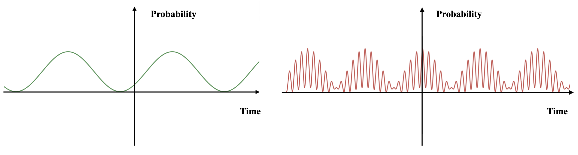
Figure 1: Quantum clocks with equally weighted eigenfunctions and two (left panel) or three (right panel) energy levels.

Let us now consider the case when the system has infinitely many different energy levels. If these are all exact eigenstates of the Hamiltonian, we can set up states which will cycle between different constituents regularly, as if the number of levels were finite. We are not interested in such cases, since they do not really add anything new to the discussion. Instead, to define what we are interested in, let us consider the example provided by Hydrogen atom, and its dynamics. In non-relativistic quantum mechanics, Hydrogen atom is described by the Hamiltonian

$$H=-\frac{1}{2m}\vec{\nabla}^{2}-\frac{\alpha}{|\vec{r}\,|}\,,$$ (11)

and has infinitely many discrete bound states, whose energies are

$$E_{n}=-\frac{R}{n^{2}}\,,~{}~{}~{}~{}~{}~{}n=1,2,3,\ldots$$ (12)

where $R=m\alpha^{2}/2$ is the Rydberg constant for Hydrogen atom, and $\alpha=e^{2}/4\pi\simeq 1/137$ the fine structure constant. Each level is $2n^{2}$ times degenerate, due to spin and the conserved Lenz vector, which enhances the manifest $O(3)$ symmetry to $O(4)$. At first glance, since $H$ in (11) is Hermitean, the energies $E_{n}$ are real, and so the eigenstates $|\psi_{n}\rangle$ are absolutely stable. If we took any individual energy eigenstate, it would never change by Hamiltonian-induced translation. Likewise, if we took a generic linear combination of them as an initial state, it would seem to cycle between different constituents without an end – the situation which we just declared a lack of interest in.

However, this is incorrect. The standard textbook description of Hydrogen in nonrelativistic limit is just an approximation. The full quantum state of Hydrogen must also specify the state of photons, not only the electron, since its charge is nonzero and the photon is massless. A generic state of the atom is given by a linear combination of direct product states $\propto|{\rm electron}\rangle\otimes|{\rm photon}\rangle$. The photon states are not the photon vacuum.

We can describe what happens by recalling that Coulomb potential in the Hydrogen Lagrangian comes from the timelike components in the covariant interaction

$$A_{\mu}\bar{\psi}\gamma^{\mu}\psi=A_{0}\psi^{\dagger}\psi+\ldots\,,$$ (13)

in nonrelativistic limit. The vector $A_{\mu}$ is the quantized photon field, and the Coulomb potential is its expectation value between in- and out-photon states. If in perturbation theory the photon state were an empty vacuum of $A_{\mu}$, this would be zero. Instead, the photon state in Hydrogen atom must be a coherent state $|{\cal C}\rangle\propto\sum_{n}c_{n}|n~{}{\rm photons}\rangle$ [18, 19], such that $\langle{\cal C}|A_{0}|{\cal C}\rangle=-{\alpha}/{|\vec{r}\,|}$. Once this is included, the full gauge invariant perturbation theory description of Hydrogen requires replacing $-i\vec{\nabla}\rightarrow-i\vec{\nabla}+e\vec{A}$, and the vector potential fluctuation can be taken to be in the Coulomb gauge, $\phi=0$, $\vec{\nabla}\cdot\vec{A}=0$. The operator $\propto\vec{A}\cdot\vec{\nabla}$ mediates the decay of excited states to the ground state, triggering spontaneous emission.

This phenomenon is purely quantum-mechanical. A variant of it has been found experimentally by L. Meitner [20] (in nuclear physics) and, independently, P. Auger [21] (in atomic physics). The precise theory of it is based on the article by Dirac which initiated the foundation of quantum field theory [22], which showed the decay rate, as confirmed shortly later in the papers [23, 24] by Weisskopf and Wigner. A nice summary can be found in [25, 26].

And yet the main result was correctly calculated by Albert Einstein, almost a decade prior, before the glimpses of quantum field theory, and before the experimental discoveries of Meitner and Auger. Einstein presciently anticipated the phenomenon of spontaneous emission [27] in 1917, in his rederivation of Planck’s black body spectrum of radiation. We summarize this remarkable work here, following delightful lectures by Tong [28].

Einstein started with a system of atoms immersed in a reservoir of photons, and assumed that the system is in thermal equilibrium. He allowed that atoms and photons interact, and that atoms can both absorb and emit photons, by having an electron change the level. He further observed that the absorption and emission are amplified in environments where the radiator is surrounded by photons, but also included a channel where an excited, higher energy, atom state can decay into a lower energy, ground, state, by releasing a photon even in the empty reservoir. In ter Haar’s translation of Einstein’s original article [27], Einstein stated

Accordingly, let it be possible for a molecule to make without external stimulation a transition from the state $Z_{m}$ to the state $Z_{n}$ while emitting the radiation of energy $\varepsilon_{m}-\varepsilon_{n}$ of frequency $\nu$.

Two lines below, Einstein introduced his famous $A$-coefficient, measuring the rate of this transition. The inclusion of this parameter opened up the possibility of spontaneous emission, with the calculation to provide the check if it is nonzero. The reverse process, of spontaneous excitation, was ignored from the outset, as it were. Ignoring it is fully justified: if there were no photons anywhere near an atom in the ground state, it could self-excite only by emitting a photon of $\omega<0$ – an obvious affront to physics to and fro (and a reminder that Hydrogen Hamiltonian is bounded from below).

As noted above, Einstein also added the stimulated emission and absorption processes, whereby the atoms emit and absorb into/from the environment photon population, which are proportional to the number of environment photons per unit volume $n_{\gamma}$, and occur between excited and ground states with energies $E_{e}-E_{g}=\omega$. The subscripts $e$ and $g$ refer to the excited and ground state. As noted above, we take all units to be natural, so $\hbar=k_{\tt B}=c=1$. Using the principle of detailed balance for reactions, with the probability for the emission and absorption of a single photon being $B_{eg}$ for an excitation (the transition $g\rightarrow e$) and $B_{ge}$ for a relaxation ($e\rightarrow g$),

$$\delta N_{e}=n_{\gamma}(\omega)\Bigl{(}B_{eg}N_{g}-B_{ge}N_{e}\Bigr{)}-A_{ge}N_{e}\,,~{}~{}~{}~{}~{}~{}\delta N_{g}=-n_{\gamma}(\omega)\Bigl{(}B_{eg}N_{g}-B_{ge}N_{e}\Bigr{)}+A_{ge}N_{e}\,.$$ (14)

For a system in equilibrium, $\delta N_{e}=\delta N_{g}=0$, and so

$$n_{\gamma}(\omega)=\frac{A_{ge}N_{e}}{B_{eg}N_{g}-B_{ge}N_{e}}=\frac{\frac{A_{ge}}{B_{ge}}}{\frac{B_{eg}}{B_{ge}}\frac{N_{g}}{N_{e}}-1}\,.$$ (15)

Further, in equilibrium the populations of modes with energy $E$ obey Maxwell-Boltzmann distribution, so that

$$\frac{N_{e}}{N_{g}}=\frac{g_{e}e^{-E_{e}/T}}{g_{g}e^{-E_{g}/T}}=\frac{g_{e}}{g_{g}}\,e^{-\omega/T}\,.$$ (16)

The numbers $g_{g}$ and $g_{e}$ are degeneracies (in energy) of the ground and excited states. Substituting this into (15), we reproduce Planck’s formula for photon distribution iff

$$B_{eg}\,g_{g}=B_{ge}\,g_{e}\,,~{}~{}~{}~{}~{}~{}~{}~{}~{}~{}~{}~{}A_{ge}=\frac{\omega^{3}}{\pi^{2}}B_{ge}\,.$$ (17)

Thus if we calculate e.g. $B_{ge}$ from first principles, all other parameters are determined. We could get a possible leading contribution to $B_{ge}$ by immersing a Hydrogen in a weak, spatially uniform, randomly oriented harmonic electric field, with a Planck’s distribution of frequencies and a random field orientation. This will excite the atom, inducing Rabi oscillations [28], with the probability

$$P_{e}=\frac{8\pi\alpha}{3}|\langle e|\vec{r}|g\rangle|^{2}\int d\omega\frac{n_{\gamma}(\omega)}{(\omega-\omega_{0})^{2}}\sin^{2}\bigl{(}\frac{(\omega-\omega_{0})t}{2})\bigr{)}\,,$$ (18)

where $E_{e}-E_{g}=\omega_{0}$ and $1/3$ arises from directional averaging. After evaluating the integral using contour techniques, the result gives the width $B_{ge}=dP_{e}/dt$,

$$B_{ge}=\frac{4\pi^{2}\alpha}{3}|\langle e|\vec{r}|g\rangle|^{2}\,.$$ (19)

Thus the spontaneous emission rate is

$$A_{ge}=\frac{4\alpha\omega^{3}}{3}|\langle e|\vec{r}|g\rangle|^{2}\,.$$ (20)

Note, that $|\langle e|\vec{r}|g\rangle|^{2}$ could vanish for some states $e$, by symmetry, leading to specific selection rules allowing or prohibiting some transitions. However this does not imply the stability of the state $e$; instead, other channels can occur, mediated by higher multipoles in the expansion, or via indirect processes $e\rightarrow e^{\prime}\rightarrow\ldots\rightarrow g$, whereby $e$ decays to the ground state in steps. The only stable state is the ground state.

Had the Hamiltonian not been bounded from below, the decay process to ever lower energy states would have continued indefinitely, and so the time reversal $t\rightarrow-\infty$ would have looked just like the original tower of transitions. However just having a lowest energy state is not sufficient to guarantee time’s arrow. A case in point is precisely the aforementioned Jaynes-Cummings model [15], which describes a two-state “atom” interacting with a quantized “photon field” of a single fixed frequency (and a discretely infinite spectrum above it), enclosed in a cavity. Even though the system has a spectrum bounded from below, it does not have a definite arrow of time. The Hamiltonian eigenfunctions of this system are not the atom “flavor” eigenfunctions, and so during evolution an atom ground state can spontaneously interact with the photon and become excited again, leading to the periodic process of quantum collapse and quantum revival [16]. Heuristically, one might think of this as being due to the previously emitted photons, which never leave the cavity, “bounce” off the walls, and every so often re-excite an atom in the ground state.

As the cavity walls are moved out the revival delay increases. Eventually, with the full removal of the wall, and restoration of the full continuum of free photons which can escape to infinity, there will be no revival. The Hydrogen ground state will then be a quantum attractor of evolution, and together with a huge number of decay channels taking energy to infinity, it will manifestly remove any semblance of universal $t\leftrightarrow-t$ symmetry – finally inducing a definite arrow of time.

Further, note that in the formula (20) all the reference to thermal equilibrium and the reservoir of photons has completely disappeared. The equation is completely microscopic and local, applying to a single isolated Hydrogen atom. Many authors in quantum field theory have stressed this repeatedly, based on the original papers calculating spontaneous emission rate in quantum field theory [22, 23, 24]. This is reflected in the textbooks and lectures, too [25, 26, 28]. While it is certainly true that (20) can be correctly calculated without ever invoking statistical notions, Einstein’s prescient argument [27] feels too elegant to be a mere accident. Since the consistent description of Hydrogen requires deploying coherent photon states [18, 19], it is tempting to imagine that the description of the evolution of the coherent state describing the photon sector in spontaneous emission could be the process of entanglement initiated by the emitted photon evacuating to infinity, in a way proposed in [30, 31] to describe the equilibration of a complex quantum system. Even for a single atom, the coherent state involves contributions from many photons, and so this possibility seems like an intriguing avenue to explore.

While we have focused above on Hydrogen, it should be clear that the conclusions apply equally well to other atoms and molecules. As long as they have Hamiltonians bounded from below and interact with photons (or other continua of mediators), the ground state will be the quantum attractor. So if we ignore gravity, we can imagine an ensemble of such clocks distributed around the universe at any particular time, as defined by any particular observer, and they will all locally pick the same arrow of time, as dictated by evolution. If on the other hand we include gravity, we can wonder if by making the distribution of clocks very dense somewhere we might get gravitational effects to tilt, and maybe even invert time’s arrow. That can indeed happen; perhaps the simplest example is Schwarzschild black hole,

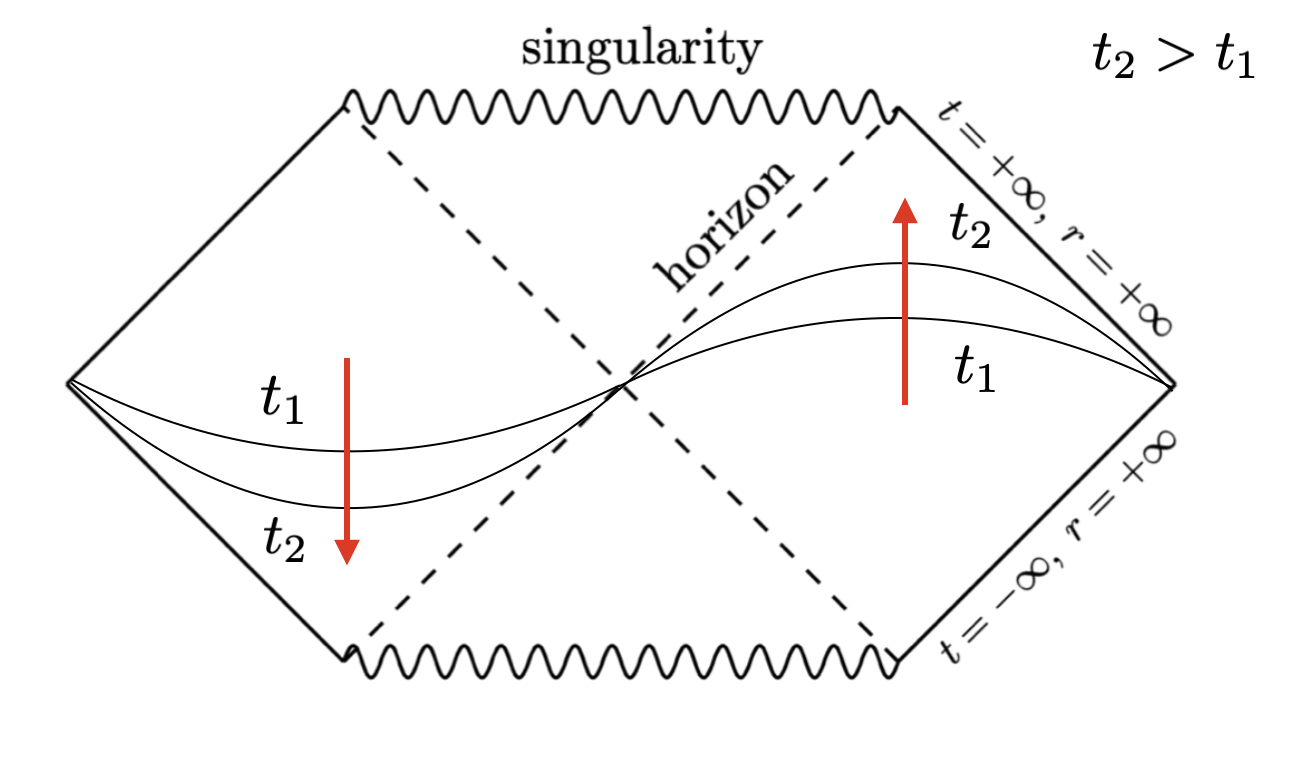
Figure 2: Schwarzschild time reversal, with the local time arrows shown in red.

where the gravitational effects flip the coordinate time direction from one asymptotic infinity to another. However the observers who are experiencing opposite time arrows are separated by event horizons, and so they cannot causally communicate the flip to each other, at least classically. Quantum mechanically, the answer is still behind the veils covering Hawking’s radiation [32]. This behavior seems universal under generic conditions, given Hawking’s chronology protection conjecture [33]. While gravity can flip time’s arrow along spacelike surfaces, classical observers cannot see that due to the causal barriers posed by horizons.

Time’s arrow in cosmology and its connection to inflation is another set of open questions [1, 2, 3, 4, 5, 6, 7, 8]. A big additional problem which adds to the confusion is that the analogue to the Hamiltonian with gravity included is the ADM Hamiltonian density which vanishes identically for all spacetimes: ${\cal H}_{ADM}=0$ [34]. Thus there is no obvious candidate for time, let alone its arrow. Nevertheless, in the subspace of de Sitter spaces, in theories where cosmological constant can be screened by fluxes of $4$-forms, there is a tendency of a de Sitter space of high curvature to decay to a de Sitter space of lower curvature [35, 36]. Under certain quite general conditions [37, 38, 39, 40], when the flux terms screening the cosmological constant are dominated by linear terms, the vanishing cosmological constant and the associated Minkowski space are the unique quantum attractor. This behavior is analogous to the ground state of Hydrogen. This feature might well be a factor in the emergence of time’s arrow in at least spacetimes which include de Sitter sections. In this case, the universe could start as a rare random fluctuation [41, 42] from flat space [8], which unlike the spontaneous excitement of an atom could occur because ${\cal H}_{ADM}=0$, so that there is no energy barrier, but then it evolves back toward Minkowski. This might correlate the smallness of the cosmological constant with cosmic time’s arrow. We think that these are interesting issues, and intend to return to them elsewhere. “Time Is on My Side” comes to mind.

Acknowledgments: We would like to thank A. Albrecht, G. D’Amico, and A. Westphal for useful discussions. NK is supported in part by the DOE Grant DE-SC0009999.

References

- [1] T. Gold, American Journal of Physics 30, 403-410 (1962).
- [2] R. Penrose, “Singularities and time-asymmetry,”, in General Relativity: An Einstein Centenary Survey, edited by S. Hawking and W. Israel, Cambridge University Press, Cambridge UK 1979.
- [3] P. C. W. Davies, Nature 301, 398-400 (1983).
- [4] D. N. Page, Nature 304, 39-41 (1983).
- [5] P. C. W. Davies, Nature 312, 524-527 (1984).
- [6] R. Penrose, Annals N. Y. Acad. Sci. 571, 249-264 (1989).
- [7] A. Albrecht, [arXiv:astro-ph/0210527 [astro-ph]].
- [8] S. M. Carroll and J. Chen, [arXiv:hep-th/0410270 [hep-th]].
- [9] V. I. Yukalov, Phys. Lett. A 308, 313-318 (2003) [arXiv:cond-mat/0303497 [cond-mat]].
- [10] J. F. Donoghue and G. Menezes, Prog. Part. Nucl. Phys. 115, 103812 (2020) [arXiv:2003.09047 [quant-ph]].
- [11] J. Fröhlich, [arXiv:2202.04619 [quant-ph]].
- [12] A. Messiah, Quantum Mechanics vols. I II, Dover, Mineola, NY 1999.
- [13] L. Susskind and J. Glogower, Physics Physique Fizika 1, no.1, 49-61 (1964).
- [14] P. Carruthers and M. M. Nieto, Rev. Mod. Phys. 40, 411-440 (1968).
- [15] E. T. Jaynes and F. W. Cummings, IEEE Proc. 51, 89-109 (1963).
- [16] J. H. Eberly, N. B. Narozhny and J. J. Sanchez-Mondragon, Phys. Rev. Lett. 44, 1323-1326 (1980).
- [17] L. Dyson, M. Kleban and L. Susskind, JHEP 10, 011 (2002) [arXiv:hep-th/0208013 [hep-th]].
- [18] R. J. Glauber, Phys. Rev. 131, 2766-2788 (1963).
- [19] J. R. Klauder, J. Phys. A 29, L293-L298 (1996) [arXiv:quant-ph/9511033 [quant-ph]].
- [20] L. Meitner, Z. Physik 9, 131-144 (1922).
- [21] P. Auger, C.R.A.S. 177, 169-171 (1923).
- [22] P. A. M. Dirac, Proc. Roy. Soc. Lond. A 114, 243 (1927).
- [23] V. Weisskopf and E. P. Wigner, Z. Phys. 63, 54-73 (1930).
- [24] V. Weisskopf and E. P. Wigner, Z. Phys. 65, 18-29 (1930).
- [25] M. Sargent III, M. O. Scully, W. E. Lamb, Laser Physics, Addison-Wesley Publishing Co., Reading, MA 1974.
- [26] C. C. Gerry, P. L. Knight, Introductory Quantum Optics, Cambridge University Press, Cambridge UK 2005.
- [27] A. Einstein, Phys. Z. 18, 121-128 (1917).
- [28] D. Tong, Lectures on Applications of Quantum Mechanics, Part II Cambridge Tripos.
- [29] N. Bohr, Phil. Mag. Ser. 6 26, 1-24 (1913).
- [30] P. Reimann, Phys. Rev. Lett. 101, 190403 (2008) [arXiv:0810.3092 [cond-mat.stat-mech]].
- [31] N. Linden, S. Popescu, A. J. Short and A. Winter, Phys. Rev. E 79, no.6, 061103 (2009) [arXiv:0812.2385 [quant-ph]].
- [32] S. W. Hawking, Nature 248, 30-31 (1974).
- [33] S. W. Hawking, Phys. Rev. D 46, 603-611 (1992).
- [34] R. L. Arnowitt, S. Deser and C. W. Misner, Gen. Rel. Grav. 40, 1997-2027 (2008) [arXiv:gr-qc/0405109 [gr-qc]].
- [35] J. D. Brown and C. Teitelboim, Phys. Lett. B 195, 177-182 (1987).
- [36] J. D. Brown and C. Teitelboim, Nucl. Phys. B 297, 787-836 (1988).
- [37] N. Kaloper, Phys. Rev. D 106, no.6, 065009 (2022) [arXiv:2202.06977 [hep-th]].
- [38] N. Kaloper, Phys. Rev. D 106, no.4, 044023 (2022) [arXiv:2202.08860 [hep-th]].
- [39] N. Kaloper and A. Westphal, Phys. Rev. D 106, no.10, L101701 (2022) [arXiv:2204.13124 [hep-th]].
- [40] N. Kaloper, [arXiv:2305.02349 [hep-th]].
- [41] E. P. Tryon, Nature 246, 396 (1973).
- [42] J. Garriga and A. Vilenkin, Phys. Rev. D 57, 2230-2244 (1998) [arXiv:astro-ph/9707292 [astro-ph]].