Revisiting Weak Energy Condition and wormholes in Brans-Dicke gravity

Abstract

It is known that the formation of a wormhole typically involves a violation of the Weak Energy Condition (WEC), but the reverse is not necessarily true. In the context of Brans-Dicke gravity, the generalized Campanelli-Lousto solution, which we shall unveil in this paper, demonstrates a WEC violation that coincides with the appearance of unbounded sheets of spacetime within the “interior” section. The emergence of a wormhole in the “exterior” section is thus only an indirect consequence of the WEC violation. Additionally, we use the generalized Campanelli-Lousto solution to construct a Kruskal-Szekeres diagram, which exhibits a “gulf” sandwiched between the four quadrants in the diagram, a novel feature in Brans-Dicke gravity. Overall, our findings shed new light onto a complex interplay between the WEC and wormholes in the Brans-Dicke theory.

I Introduction

Wormholes are hypothetical spacetime structures that may interact with ordinary matter and thus can be observed and even distinguished from black holes [1, 2, 3, 4, 5, 6, 7, 8, 9, 10, 11, 12, 13, 14, 15].

To maintain a wormhole, it is necessary to violate the Weak Energy Condition (WEC) [16, 17, 19, 20, 18]. In its geometric form, the WEC requires that

$$G_{\mu\nu}\,t^{\mu}t^{\nu}\geq 0$$ (1)

for every future-pointing timelike vector $t^{\mu}$. Specifically, for the vector $t^{\mu}=(1,0,0,0)$, the WEC yields $G_{00}\geq 0$, meaning positive energy density everywhere in any frame of reference. In general relativity (GR), exotic matter that is equivalent to a negative energy density is needed in order to violate the WEC. Nevertheless, in generalized or modified theories of GR, the WEC may be violated via the introduction of extra terms or corrections to the gravitation sector, which can play the role of exotic matter without truly being exotic matter.

An example of a theory that supports a wormhole is the Brans-Dicke (BD) action. In [21] Agnese and La Camera used the Campanelli-Lousto vacuum solution [22] to show that the BD theory produces a wormhole when the post-Newtonian parameter $\gamma>1$ and a naked singularity when $\gamma<1$. They also found that the combination $(1-\gamma)(1+2\gamma)/(1+\gamma)$ determines the sign of $G_{00}$. While the WEC is indeed violated when a wormhole is formed $(\gamma>1)$, the reverse is not necessarily true, as a violation can also occur when $-1<\gamma<-1/2$, in which case no wormhole is formed.

In this paper, we revisit the analysis of Agnese-La Camera and delve further into the WEC in the BD theory, aiming to answer the question of what happens to spacetime in the absence of a wormhole when the WEC is violated. Our findings for BD gravity may have broader implications for modified gravity theories at large [25, 24, 26, 27, 23, 28, 29].

The paper is structured as follows. Section II reviews and generalizes the existing Campanelli-Lousto (CL) solution so that it is also valid for the interior region. Section III analyzes the generalized CL solution, including the wormhole it produces. Section IV explores the violation of the WEC. Section V relates the special Buchdahl-inspired metric uncovered and examined in Refs.  [30, 33, 31, 32] with the generalized CL metric. Section VI constructs a Kruskal-Szekeres diagram for the latter metric. Appendix A gives a brief overview of the Brans solutions, while Appendix B validates the generalized CL solution via direct inspection.

II Extension of the Campanelli-Lousto solution

We shall consider the original Brans-Dicke (BD) action [34]

$$\int d^{4}x\sqrt{-g}\left[\phi\,\mathcal{R}-\frac{\omega}{\phi}g^{\mu\nu}\partial_{\mu}\phi\partial_{\nu}\phi\right]$$ (2)

Its field equations are given by

$$\mathcal{R}_{\mu\nu}-\frac{1}{2}g_{\mu\nu}\mathcal{R} =\frac{1}{\phi}\left(\nabla_{\mu}\nabla_{\nu}\phi-g_{\mu\nu}\square\,\phi\right)$$

$$\ \ \ +\frac{\omega}{\phi^{2}}\Bigl{(}\nabla_{\mu}\phi\nabla_{\nu}\phi-\frac{1}{2}g_{\mu\nu}(\nabla\phi)^{2}\Bigr{)}$$ (3)

$$(2\omega+3)\,\square\,\phi =0$$ (4)

and the Ricci scalar is

$$\mathcal{R}=\frac{\omega}{\phi^{2}}\,(\nabla\phi)^{2}$$ (5)

In his PhD thesis on the BD field equations, Brans discovered four solutions, which he reported in Ref.  [35]. These solutions are expressed in isotropic coordinates and named type I, II, III, and IV, respectively. Among these four solutions, the Brans type I solution has been the most explored one, with the other three solutions being “derivable” from it via duality or by taking a proper limit, as we shall discuss in Appendix A. In what follows, we adopt the notation in Agnese and La Camera [21], who were the first researchers to correctly expose the wormhole and naked singularity from the Campanelli-Lousto solution , which is in essence the Brans type I solution expressed in a different coordinate system [22, 36].

The Brans type I solution comprises of a metric

$$ds_{\text{Brans-I}}^{2} =-\left|\frac{1-\frac{r_{\text{s}}}{4\bar{r}}}{1+\frac{r_{\text{s}}}{4\bar{r}}}\right|^{2A}dt^{2}$$

$$+\left(1-\frac{r_{\text{s}}^{2}}{16\bar{r}^{2}}\right)^{2}\left|\frac{1-\frac{r_{\text{s}}}{4\bar{r}}}{1+\frac{r_{\text{s}}}{4\bar{r}}}\right|^{2B}\left(d\bar{r}^{2}+\bar{r}^{2}d\Omega^{2}\right)$$ (6)

and a scalar field

$$\phi_{\text{Brans-I}}=\phi_{0}\left|\frac{1-\frac{r_{\text{s}}}{4\bar{r}}}{1+\frac{r_{\text{s}}}{4\bar{r}}}\right|^{-(A+B)}$$ (7)

with $\bar{r}$ being the isotropic radial coordinate, and $d\Omega^{2}=d\theta^{2}+\sin^{2}\theta\,d\varphi^{2}$ the line element on the unit 2-sphere. In terms of $A$ and $B$, the Brans-Dicke coupling parameter is

$$\omega=-2\,\frac{A^{2}+AB+B^{2}-1}{(A+B)^{2}}$$ (8)

Since $\omega$ is a parameter of the action, the Brans type I solution effectively involves three parameters, $r_{\text{s}}$, $\phi_{0}$ and either $A$ or $B$ (related to each other via $\omega$). The Ricci scalar curvature

$$\mathcal{R}=-(A^{2}+AB+B^{2}-1)\frac{128\,r_{\text{s}}^{-2}}{\left(\frac{4\bar{r}}{r_{\text{s}}}-\frac{r_{\text{s}}}{4\bar{r}}\right)^{4}}\left|\frac{1-\frac{r_{\text{s}}}{4\bar{r}}}{1+\frac{r_{\text{s}}}{4\bar{r}}}\right|^{-2B}$$ (9)

Note that the point $\{A=1,\,B=-1\}$ is the Schwarzschild metric.

A slightly more illuminating expression can be obtained by “diagonalizing” $A$ and B, namely

$$A_{\pm}:=\frac{1}{2}(A\pm B)$$ (10)

In this notation, the metric is

$$ds_{\text{Brans-I}}^{2} =\left|\frac{1-\frac{r_{\text{s}}}{4\bar{r}}}{1+\frac{r_{\text{s}}}{4\bar{r}}}\right|^{2A_{+}}\times\Biggl{\{}-\left|\frac{1-\frac{r_{\text{s}}}{4\bar{r}}}{1+\frac{r_{\text{s}}}{4\bar{r}}}\right|^{2A_{-}}dt^{2}$$

$$+\left(1-\frac{r_{\text{s}}^{2}}{16\bar{r}^{2}}\right)^{2}\left|\frac{1-\frac{r_{\text{s}}}{4\bar{r}}}{1+\frac{r_{\text{s}}}{4\bar{r}}}\right|^{-2A_{-}}\left(d\bar{r}^{2}+\bar{r}^{2}d\Omega^{2}\right)\Biggr{\}}$$ (11)

and a scalar field is

$$\phi_{\text{Brans-I}}=\phi_{0}\left|\frac{1-\frac{r_{\text{s}}}{4\bar{r}}}{1+\frac{r_{\text{s}}}{4\bar{r}}}\right|^{-2A_{+}}$$ (12)

The conformal factor in the metric is a reciprocal of the scalar field. The proper part of the metric is non-Schwarzschild if $A_{-}\neq 1$. The Ricci scalar is

$$\mathcal{R}=\frac{256\,\omega A_{+}^{2}r_{\text{s}}^{-2}}{\left(\frac{4\bar{r}}{r_{\text{s}}}-\frac{r_{\text{s}}}{4\bar{r}}\right)^{4}}\left|\frac{1-\frac{r_{\text{s}}}{4\bar{r}}}{1+\frac{r_{\text{s}}}{4\bar{r}}}\right|^{-2A_{+}+2A_{-}}$$ (13)

The relation between parameters is simplified to

$$(2\omega+3)A_{+}^{2}+A_{-}^{2}=1$$ (14)

The generalized Campanelli-Lousto solution

From the Brans type I solution, one can obtain the Campanelli-Lousto solution [22]. To see this, let us make the following coordinate transformation

$$r=\bar{r}\left(1+\frac{r_{\text{s}}}{4\bar{r}}\right)^{2}\geqslant r_{\text{s}}$$ (15)

or, equivalently

$$\left(\frac{1-\frac{r_{\text{s}}}{4\bar{r}}}{1+\frac{r_{\text{s}}}{4\bar{r}}}\right)^{2}=1-\frac{r_{\text{s}}}{r}$$ (16)

For each value of $r>r_{\text{s}}$ there exist two distinct values $\bar{r}_{1}$ and $\bar{r}_{2}$ such that $\frac{4\bar{r}_{1}}{r_{\text{s}}}=\frac{r_{\text{s}}}{4\bar{r}_{2}}$, corresponding two symmetric exterior sheets of spacetime. In the radial coordinate $r$, the Brans type I solution becomes the metric [22]

$$ds^{2} =-\left(1-\frac{r_{\text{s}}}{r}\right)^{A}dt^{2}+\left(1-\frac{r_{\text{s}}}{r}\right)^{B}dr^{2}+\left(1-\frac{r_{\text{s}}}{r}\right)^{B+1}r^{2}d\Omega^{2}$$ (17)

and the scalar field

$$\phi(r) =\phi_{0}\left(1-\frac{r_{\text{s}}}{r}\right)^{-\frac{1}{2}(A+B)}$$ (18)

which together comprise the Campanelli-Lousto (CL) solution. It is important to note that the above expressions, as originally reported in [22], are only applicable for the “exterior”, viz. $r>r_{\text{s}}$. They are not valid if $A$ or $B$ takes on a non-integer value.

However, it is a straightforward exercise to verify by direct inspection that the following generalized CL metric

$$ds^{2} =-\left|1-\frac{r_{\text{s}}}{r}\right|^{A-1}\left(1-\frac{r_{\text{s}}}{r}\right)dt^{2}$$

$$\ \ \ +\left|1-\frac{r_{\text{s}}}{r}\right|^{B+1}\left[\frac{dr^{2}}{1-\frac{r_{\text{s}}}{r}}+r^{2}d\Omega^{2}\right]$$ (19)

and its associated scalar field

$$\phi(r) =\phi_{0}\left|1-\frac{r_{\text{s}}}{r}\right|^{-\frac{1}{2}(A+B)}$$ (20)

form a solution to the vacuo field equations (3)–(4) for all values of $r\in\mathbb{R}\backslash\{0,r_{\text{s}}\}$. The verification is carried out in Appendix B in details . Obviously, the generalized CL solution (19)–(20) reproduces the CL solution (17)–(18) for the “exterior”, $r>r_{\text{s}}$, but it is also applicable for the “interior” $0<r<r_{\text{s}}$ as well. It also recovers the Schwarzschild metric when $\{A=1,\,B=-1\}$.

In the generalized CL metric, $g_{tt}$ and $g_{rr}$ flip their sign across $r=r_{\text{s}}$ as desired, and the Ricci scalar is

$$\mathcal{R}=-(A^{2}+AB+B^{2}-1)\frac{r_{\text{s}}^{2}}{2r^{4}}\left|1-\frac{r_{\text{s}}}{r}\right|^{-B-2}\text{sgn}\left(1-\frac{r_{\text{s}}}{r}\right)$$ (21)

It should be noted that although along the line $A+B=0$, $\phi$ is a constant, the value of $\omega$ is infinite (except at the Schwarzschild point $\{A=1,\,B=-1\}$); this explains why the metric can deviate from the Schwarzschild metric.

In terms of $A_{\pm}:=\frac{1}{2}(A\pm B)$, the metric and the scalar field are

$$ds^{2} =\left|1-\frac{r_{\text{s}}}{r}\right|^{A_{+}}\biggl{\{}-\left|1-\frac{r_{\text{s}}}{r}\right|^{A_{-}-1}\left(1-\frac{r_{\text{s}}}{r}\right)dt^{2}$$

$$\ \ \ +\left|1-\frac{r_{\text{s}}}{r}\right|^{-A_{-}+1}\biggl{[}\frac{dr^{2}}{1-\frac{r_{\text{s}}}{r}}+r^{2}d\Omega^{2}\biggr{]}\biggr{\}},$$ (22)

and

$$\phi(r)=\phi_{0}\left|1-\frac{r_{\text{s}}}{r}\right|^{-A_{+}}.$$ (23)

The conformal factor of the metric is a reciprocal of the scalar field, whereas the proper part of the metric is specified by $A_{-}$ but not $A_{+}$.

III Properties of the generalized Campanelli-Lousto solution

III.1 Casting in the Morris-Thorne ansatz

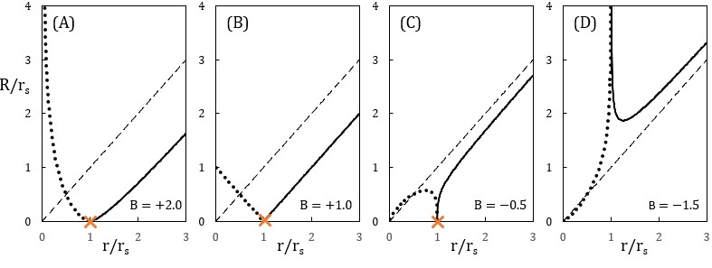
Figure 1: Behavior of the areal radius, $R/r_{\text{s}}$, for the generalized Campanelli-Lousto metric versus $r/r_{\text{s}}$. Panel D, representative of $B<-1$, yields a minimum for $R(r)$ and corresponds to a wormhole “throat”. Note that the horizon at $r=r_{\text{s}}$ is non-singular only if $\{B\leq-2\}$ or $\{B=-1$ and $A\in\{0,1\}\}$. Some of the plots have been extended to $r<r_{\text{s}}$ even when the horizon is singular, shown as crosses, with the extension shown in dotted segments. For benchmarking, the dashed lines $R=r$ are the Schwarzschild metric, $\{B=-1$ and $A=1\}$.

In this section, we shall bring metric (19) to the Morris-Thorne ansatz [17]

$$ds^{2}=-e^{2\Phi(R)}dt^{2}+\frac{dR^{2}}{1-\frac{b(R)}{R}}+R^{2}d\Omega^{2}$$ (24)

As a function of $r$, the areal radius is

$$R(r) =r\left|1-\frac{r_{\text{s}}}{r}\right|^{\frac{1}{2}(B+1)}$$ (25)

leading to

$$\frac{dR}{dr}=\text{sgn}\left(1-\frac{r_{\text{s}}}{r}\right)\left|1-\frac{r_{\text{s}}}{r}\right|^{\frac{B-1}{2}}\left[1+\frac{B-1}{2}\frac{r_{\text{s}}}{r}\right]$$ (26)

The redshift function $\Phi(R)$ is defined via

$$e^{2\Phi(R)}=\text{sgn}\left(1-\frac{r_{\text{s}}}{r}\right)\left|1-\frac{r_{\text{s}}}{r}\right|^{A}$$ (27)

and the shape function $b(R)$ via

$$1-\frac{b(R)}{R}=\frac{1}{1-\frac{r_{\text{s}}}{r}}\left[1+\frac{B-1}{2}\frac{r_{\text{s}}}{r}\right]^{2}$$ (28)

with $r$ being implicit function of $R$ via Eq. (25). The behavior of $R(r)$ is shown in Fig. 1. In the exterior, $R(r)$ exhibits a minimum for $B<-1$ (represented by Panel D in Fig. 1).

In addition, the asymptotic behaviors of the areal radius are

$$R\simeq\begin{cases}r&\text{as }r\rightarrow\infty\\ \left|r-r_{\text{s}}\right|^{\frac{1}{2}(1+B)}&\text{as }r\rightarrow r_{\text{s}}\\ r^{\frac{1}{2}(1-B)}&\text{as }r\rightarrow 0\end{cases}$$ (29)

We must note in advance that the graphs shown in Fig. 1 are only “half” of the story. There is a maximal analytic extension of the generalized CL metric via the Kruskal-Szekeres (KS) diagram, to be constructed in Section VI. The KS diagram “doubles” the coverage of the generalized CL solution, in addition to uncovering a “gulf” sandwiched between the four quadrants.

III.2 The four Morris-Thorne constraints

Let us restrict our consideration to the range $B<-1$, of which Panel (D) in Fig. 1 is a representative.

• The areal radius $R$ diverges at $r=r_{\text{s}}$ when $B<-1$.

• The equation $\frac{dR}{dr}=0$ in (26) has a single root

  $$r_{*}=\frac{1-B}{2}\,r_{\text{s}}>r_{\text{s}}\ \ \ \text{when }B<-1$$ (30)

  with $R$ attaining a miminum value

  $$R_{*} =\frac{r_{\text{s}}}{2}\sqrt{1-B^{2}}\left(\frac{1+B}{1-B}\right)^{\frac{B}{2}}$$ (31)

It is straightforward to verify that when $B<-1$ the four constraints for the metric to possess a wormhole are met [16, 17], as can be seen in Panel D of Fig. 1:

Constraint #1.—The redshift function $\Phi(R)$ (defined in (27)) be finite everywhere (hence no horizon).

Constraint #2.—Minimum value of the $R$-coordinate, i.e. at the throat of the wormhole, $R_{*}$ being the minimum value of $R$ per Eq. (31).

Constraint #3.—Finiteness of the proper radial distance, i.e. $b(R)/R\leq 1$ for $R\geq R_{*}$. The equality sign holds only at the throat, viz. $R=R_{*}$. Note that the condition $b(R)/R\leq 1$ assures that the metric component $g_{RR}$ does not change its sign for any $R\geq R_{*}$.

Constraint #4.—Asymptotic flatness condition, i.e. ${\displaystyle\lim_{R\rightarrow+\infty}\frac{b(R)}{R}=0}$.

III.3 Singularities

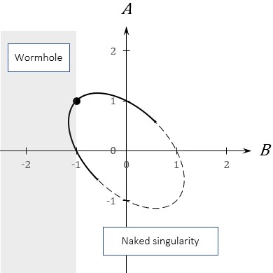
Figure 2: Parameter space of the generalized CL metric, Eq. (19). Black dot is Schwarzschild metric $\{A=1,B=-1\}$. The ellipse is the loci $A^{2}+AB+B^{2}=1$ along which the Ricci scalar $\mathcal{R}$ vanishes for all $r\in\mathbb{R}$. The vertical line $B=-1$ separates the formation of a wormhole (the shaded area) from the naked singularity (the white area). The solid curve segment on the ellipse corresponds to the asymptotically flat Buchdahl-inspired metric, discussed in Sec. V, with the two end points of the segment being ($1/\sqrt{3},\,1/\sqrt{3}$) and ($-1/\sqrt{3},\,-1/\sqrt{3}$).

The Ricci scalar:

It is given in Eq. (21). It is identically zero on the loci of an ellipse $A^{2}+AB+B^{2}=1$. See Fig. 2.

Kretschmann invariant:

For all $r\in\mathbb{R}$, the Kretschmann invariant is given by [37]

$$K :=\mathcal{R}_{\mu\nu\rho\sigma}\mathcal{R}^{\mu\nu\rho\sigma}$$ (32)

$$=4\left(\mathcal{R}_{\ \ 01}^{01}\right)^{2}+8\left(\mathcal{R}_{\ \ 02}^{02}\right)^{2}+8\left(\mathcal{R}_{\ \ 12}^{12}\right)^{2}+4\left(\mathcal{R}_{\ \ 23}^{23}\right)^{2}$$ (33)

$$=\left|1-\frac{r_{\text{s}}}{r}\right|^{-2(B+2)}\ \frac{r_{\text{s}}^{2}}{r^{6}}\,\biggl{(}6\mathfrak{A}-2\mathfrak{B}\,\frac{r_{\text{s}}}{r}+\frac{\mathfrak{C}}{4}\,\frac{r_{\text{s}}^{2}}{r^{2}}\biggr{)}$$ (34)

in which

$$\mathfrak{A} =A^{2}+B^{2}$$ (35)

$$\mathfrak{B} =A^{2}(A-2B+3)-B(B-1)(B-2)$$ (36)

$$\mathfrak{C} =(A+1)A^{2}(A-2B+3)$$

$$\ \ \ +(3A^{2}+B^{2}-2B+3)(B-1)^{2}$$ (37)

The curvature singularity at $r=r_{\text{s}}$ exists for $B>-2$ and $\{A,B\}\notin\{1,-1\}\cup\{0,-1\}$.

Case	Range for $B$	$r\rightarrow 0$	$r\rightarrow r_{\text{s}}$	$\begin{array}[]{c}\text{Wormhole or}\\ \text{naked singularity ?}\end{array}$	$\begin{array}[]{c}\text{Interior region}\\ \text{consists of ...}\end{array}$	$\begin{array}[]{c}\text{WEC}\\ \text{violation ?}\end{array}$
[I]	$B<-2$	$\begin{array}[]{c}R\text{ vanishes}\\ K\text{ diverges}\end{array}$	$\begin{array}[]{c}R\text{ diverges}\\ K\text{ vanishes}\end{array}$	Wormhole	2 unbounded sheets	Yes
[II]	$\ -2<B<-1\$	$\ \,\begin{array}[]{c}R\text{ vanishes}\\ K\text{ diverges}\end{array}\ \,$	$\ \,\begin{array}[]{c}R\text{ diverges}\\ K\text{ diverges}\end{array}\ \,$	Wormhole	2 unbounded sheets	Yes
[III]	$-1<B<1$	$\begin{array}[]{c}R\text{ vanishes}\\ K\text{ diverges}\end{array}$	$\begin{array}[]{c}R\text{ vanishes}\\ K\text{ diverges}\end{array}$	Naked singularity	4 bounded sheets	No
[IV]	$1<B<2$	$\begin{array}[]{c}R\text{ diverges}\\ K\text{ diverges}\end{array}$	$\begin{array}[]{c}R\text{ vanishes}\\ K\text{ diverges}\end{array}$	Naked singularity	2 unbounded sheets	Yes
[V]	$2<B$	$\begin{array}[]{c}R\text{ diverges}\\ K\text{ vanishes}\end{array}$	$\begin{array}[]{c}R\text{ vanishes}\\ K\text{ diverges}\end{array}$	Naked singularity	2 unbounded sheets	Yes

Table 1: Behavior of the areal radius $R$ and the Kretschmann scalar $K$ as $r$ approaches $0$ or $r_{\text{s}}$. A wormhole is formed when $R$ exhibits a minimum in the exterior region. The Weak Energy Condition (WEC) is violated if $G_{00}<0$, see Section IV.

The asymptotic behaviors of the Ricci scalar and the Kretschmann scalar, respectively, are

$$\mathcal{R}\simeq\begin{cases}\ \ \ r^{-4}&\text{as }r\rightarrow\infty\\ \left|r-r_{\text{s}}\right|^{-(B+2)}&\text{as }r\rightarrow r_{\text{s}}\\ r^{B-2}&\text{as }r\rightarrow 0\end{cases}$$ (38)

and

$$K\simeq\begin{cases}\ \ \ r^{-6}&\text{as }r\rightarrow\infty\\ \left|r-r_{\text{s}}\right|^{-2(B+2)}&\text{as }r\rightarrow r_{\text{s}}\\ r^{2(B-2)}&\text{as }r\rightarrow 0\end{cases}$$ (39)

While both quantities vanish at $r\rightarrow+\infty,$ they project singularities at $r\rightarrow 0$ or $r\rightarrow r_{\text{s}}$. In these limits, the Ricci scalar and the Kretschmann scalar show similar behaviors, that is $K\simeq\mathcal{R}^{2}$. We thus only focus on the Kretschmann invariant in the rest of the paper. There are five cases to consider:

• The Kretschmann scalar diverges at $r=0$ if $B<2$.

• The Kretschmann scalar diverges at $r=r_{\text{s}}$ if $B>-2$.

• The areal radius diverges at $r=0$ if $B>1$.

• The areal radius diverges at $r=r_{\text{s}}$ if $B<-1$, in which case, $R(r)$ also possesses a minimum in the exterior, hence forming a wormhole.

• The areal radius vanishes at $r=r_{\text{s}}$ if $B>-1$, in which case, $R(r)$ is a monotonically increasing function in the exterior. The singularity at $r=r_{\text{s }}$ is naked.

The results are summarized in Table 1 for five cases. Note that in the Table, $R$ is the areal radius, given in Eq. (25), not the Ricci scalar $\mathcal{R}$. As we stated earlier, the generalized CL metric has a maximal analytic extension which “doubles” the number of spacetime sheets. The Table also shows the Weak Energy Condition which will be discussed in Section IV.

IV Violation of the Weak Energy Condition

In its formal geometric form [23], the Weak Energy Condition requires that $G_{\mu\nu}t^{\mu}t^{\nu}\geq 0$ for every future-pointing timelike vector $t^{\mu}$. In particular, with $t^{\mu}=(1,0,0,0)$, the WEC leads to $G_{00}\geq 0$. That is to say, effectively, energy density is positive everywhere on the manifold. The WEC is violated if the energy density is negative in some region.

The generalized CL metric given in (19) has the $00-$component of the Einstein tensor

$$G_{00}=\frac{1-B^{2}}{4\,r^{4}}r_{\text{s}}^{2}\left|1-\frac{r_{\text{s}}}{r}\right|^{A-B-2}$$ (40)

Regardless of the value of $A$, $G_{00}<0$ when a “throat” is formed, viz. when $B<-1$; see Panel D in Fig. 1. The inequality $G_{00}<0$ is interpreted as a signature of negative energy density, resulted from the BD scalar field.

Effects of violation of the WEC.—The appearance of a wormhole is associated with a violation of the WEC. However, not all violations of the WEC lead to a wormhole. For example, when $B>1$, the WEC is violated ($G_{00}<0\ \ \forall r$ as shown in Eq. (40)), but a wormhole does not appear. This raises the question of what other effects a violation of the WEC can have.

Figure 1 offers an answer to this question. Panels A and D both violate the WEC, but only Panel D exhibits a wormhole, while Panel A does not. However, both panels have something in common: they both feature an unbounded sheet of spacetime in the interior region that could exist independently of the exterior region. In contrast, Panel C has a confined interior consisting of two finite-size “bubbles” glued together . Therefore, a violation of the WEC can alter the topology of spacetime, including that of the interior.

For the generalized CL metric, a violation of the WEC leads to a divergence in the cross-section area of the spacetime configuration. This observation might have a broader range of applicability in wormhole physics, beyond Brans-Dicke gravity.

The existence of a wormhole is not a direct consequence of a violation of the WEC, but rather a by-product of a divergence in the areal radius $R(r)$ at a finite value of $r$ (whether at $r=0$ or $r=r_{\text{s}}$). Thus, a violation of the WEC may or may not result in a wormhole, and only when the divergence of $R(r)$ occurs at $r_{\text{s}}$ does a wormhole form.

The interior sheet.—The Kretschmann invariant of the generalized Campanelli-Lousto metric (34) behaves as

$$K\propto\begin{cases}r^{2(B-2)}&\text{as }r\rightarrow 0\\ \left|r-r_{\text{s}}\right|^{-2(B+2)}&\text{as }r\rightarrow r_{\text{s}}\end{cases}$$ (41)

Thus $K$ diverges at $r=0$ if $B<2$, and diverges at $r=r_{\text{s}}$ if $B>-2$. Hence, for either $B<-2$ or $B>2$, the interior sheet straddles between a singularity and a singularity-free end point. Note: there is another symmetric copy of the interior region that is obtained in the Kruskal-Szekeres diagram (see Section VI) by changing $(T,X)$ into $(-T,-X)$.

V Mapping the asymptotically flat Buchdahl-inspired metric into the generalized Campanelli-Lousto metric

A particularly interesting case is the loci $A^{2}+AB+B^{2}=1$ in Fig. 2, where $\omega=0$ throughout except at ${A=+1,B=-1}$. This loci corresponds to a Brans-Dicke theory with $\omega=0$.

In this section, we aim to establish a connection between the generalized CL solution and a vacuum solution that is asymptotically flat at spatial infinity, discovered for pure $\mathcal{R}^{2}$ gravity [30]. In [31] we completed a program that was initiated by Buchdahl in [32], and discovered a class of vacuo solutions for pure $\mathcal{R}^{2}$gravity. The Buchdahl-inspired solutions are expressible in the form

$$ds^{2}=e^{k\int\frac{dr}{r\,q(r)}}\left\{p(r)\Bigl{[}-\frac{q(r)}{r}dt^{2}+\frac{r}{q(r)}dr^{2}\Bigr{]}+r^{2}d\Omega^{2}\right\}$$ (42)

in which the pair of functions $\{p(r),q(r)\}$ obey the “evolution” rules

$${\displaystyle\frac{dp}{dr}} ={\displaystyle\frac{3k^{2}}{4\,r}\frac{p}{q^{2}}};\ \ \ \frac{dq}{dr}={\displaystyle\Bigl{(}1-\Lambda\,r^{2}\Bigr{)}\,p}$$ (43)

and the Ricci scalar equals to

$$\mathcal{R}(r)\,=\,4\Lambda\,e^{-k\int\frac{dr}{r\,q(r)}}$$ (44)

These metrics possess non-constant scalar curvature and are specified by two higher-derivative parameters, $\Lambda$ and $k$. Remarkably, we further found that the evolution rules (43) is fully soluble for $\Lambda=0$. In [30] we solved the evolution rules and derived the following metric in closed analytical form

$$ds^{2} =\left|1-\frac{r_{\text{s}}}{r}\right|^{\tilde{k}}\times$$

$$\ \left\{-\left(1-\frac{r_{\text{s}}}{r}\right)dt^{2}+\frac{dr^{2}}{1-\frac{r_{\text{s}}}{r}}\frac{\rho^{4}(r)}{r^{4}}+\rho^{2}(r)d\Omega^{2}\right\}$$ (45)

with

$$\rho(r) =\zeta r_{\text{s}}\frac{\left|1-\frac{r_{\text{s}}}{r}\right|^{\frac{\zeta-1}{2}}}{1-\text{sgn}\left(1-\frac{r_{\text{s}}}{r}\right)\left|1-\frac{r_{\text{s}}}{r}\right|^{\zeta}}$$ (46)

$$\zeta :=\sqrt{1+3\tilde{k}^{2}}\ \ \ \text{and}\ \ \ \tilde{k}:=\frac{k}{r_{\text{s}}}$$ (47)

which we named the special Buchdahl-inspired metric to reflect its distinctiveness among the class of Buchdahl-inspired metrics. By virtue of $\Lambda=0$ and Eq. (44), the special metric has a vanishing Ricci scalar everywhere, viz. $\mathcal{R}\equiv 0$ $\forall r$, and is asymptotically flat.

To connect the special Buchdahl-inspired metric with the generalized CL metric, we introduce a new radial coordinate $r^{\prime}$ such that

$$1-\frac{\zeta r_{\text{s}}}{r^{\prime}}:=\text{sgn}\left(1-\frac{r_{\text{s}}}{r}\right)\left|1-\frac{r_{\text{s}}}{r}\right|^{\zeta}$$ (48)

The metric presented in (42)–(47) can be transformed into

$$ds^{2} =-\left|1-\frac{\zeta r_{\text{s}}}{r^{\prime}}\right|^{\frac{\tilde{k}+1}{\zeta}-1}\left(1-\frac{\zeta r_{\text{s}}}{r^{\prime}}\right)dt^{2}$$

$$\ \ \ +\left|1-\frac{\zeta r_{\text{s}}}{r^{\prime}}\right|^{\frac{\tilde{k}-1}{\zeta}+1}\left[\frac{dr^{\prime 2}}{1-\frac{\zeta r_{\text{s}}}{r^{\prime}}}+r^{\prime 2}d\Omega^{2}\right]$$ (49)

which is precisely with the generalized CL metric given by Eq. (19), with an “effective” Schwarzschild radius $\zeta\,r_{\text{s}}$, and the identification

$$A=\frac{\tilde{k}+1}{\zeta};\ \ \ B=\frac{\tilde{k}-1}{\zeta}$$ (50)

It is straightforward to check that the parameters defined in (50) obey the equality (given Eq. 47)

$$A^{2}+AB+B^{2}=1$$ (51)

Therefore, the special Buchdahl-inspired metric is identical with the generalized CL metric with $\omega=0$.However, it is important to note that the general Buchdahl-inspired metric presented in (42)–(44) is distinct from the generalized CL metric. The former is a vacuum solution to the pure $\mathcal{R}^{2}$ action, whereas the latter is a vacuum solution to the Brans-Dicke action. Although the pure $\mathcal{R}^{2}$ action is equivalent a scalar-tensor action, viz.

$$\int d^{4}x\sqrt{-g}\,\mathcal{R}^{2}\ \ \longrightarrow\ \ \int d^{4}x\sqrt{-g}\left[\phi\,\mathcal{R}-\frac{\phi^{2}}{2}\right]$$ (52)

this action is not identical to the Brans-Dicke action (2), even when $\omega=0$, due to the presence of the quadratic potential $\phi^{2}/2$.

The special Buchdahl-inspired metric simultaneously belongs to the general Buchdahl-inspired metric family when $\Lambda=0$ and to the generalized CL solution family when $\omega=0$, representing the intersection of the two families. As such, it is a vacuum solution to two theories at the same time:

• The $\omega=0$ Brans-Dicke theory, viz. $\int d^{4}x\sqrt{-g}\,\phi\,\mathcal{R}$. That is to say, coupled with $\phi=\phi_{0}\left|1-\frac{r_{\text{s}}}{r}\right|^{-\frac{A+B}{2}}$ (subject to the constraint $A^{2}+AB+B^{2}=1$), the special Buchdahl-inspired metric obeys the $\omega=0$ Brans-Dicke field equations, (3)–(4), in the limit of $\phi_{0}\rightarrow 0$

  $$\mathcal{R}_{\mu\nu}-\frac{1}{2}g_{\mu\nu}\mathcal{R} =\frac{1}{\phi}\left(\nabla_{\mu}\nabla_{\nu}\phi-g_{\mu\nu}\square\,\phi\right)$$ (53)

  $$\square\,\phi =0$$ (54)

• The pure $\mathcal{R}^{2}$ theory, which is equivalent to $\int d^{4}x\sqrt{-g}\,\left[\phi\,\mathcal{R}-\frac{1}{2}\phi^{2}\right]$. That is to say, the special Buchdahl-inspired metric satisfies the following field equations, in the limit of $\phi\rightarrow 0$

  $$\mathcal{R}_{\mu\nu}-\frac{1}{2}g_{\mu\nu}\mathcal{R} =\frac{1}{\phi}\left(\nabla_{\mu}\nabla_{\nu}\phi-g_{\mu\nu}\square\,\phi\right)-\frac{1}{4}g_{\mu\nu}\phi$$ (55)

  $$\phi =\mathcal{R}$$ (56)

With $A$ and $B$ identified as in (50), the special Buchdahl-inspired metric is represented by a solid curve segment in Fig.  1, which corresponds to a portion of the ellipse defined by $A^{2}+AB+B^{2}=1$.

VI Constructing Kruskal-Szekeres diagram for the generalized Campanelli-Lousto metric

In our previous work [30], we constructed the Kruskal-Szekeres diagram for the special Buchdahl-inspired vacuum solution in pure $\mathcal{R}^{2}$ gravity. As demonstrated in the preceding section, this solution has an intimate relationship with the generalized CL metric. Therefore, we can adapt the construction method from Ref.  [30] to create a Kruskal-Szekeres diagram for the generalized CL metric, with suitable adjustments. Figure 3 shows the resulting diagram, which we present in this section.

VI.1 The Kruskal-Szekeres coordinates

The tortoise coordinate $r^{*}(r)$ for the generalized CL metric is defined to satisfy

$$dr^{*}=\frac{\text{sgn}\left(1-\frac{r_{\text{s}}}{r}\right)}{\left|1-\frac{r_{\text{s}}}{r}\right|^{A_{-}}}\,dr$$ (57)

The tortoise coordinate (modulo an additive constant) involves a Gaussian hypergeometric function:

$$r^{*} =\frac{r_{\text{s}}}{1-A_{-}}\,\left|1-\frac{r_{\text{s}}}{r}\right|^{1-A_{-}}\,_{2}F_{1}\left(2,1-A_{-};2-A_{-};1-\frac{r_{\text{s}}}{r}\right)$$ (58)

Furthermore, by integrating Eq. (57), the difference (if $A_{-}\in(-1,1)$)

$$r^{*}|_{r=0}-r^{*}|_{r=r_{\text{s}}} =\int_{0}^{r_{\text{s}}}\frac{dr}{\left(\frac{r_{\text{s}}}{r}-1\right)^{A_{-}}}=\frac{\pi A_{-}r_{\text{s}}}{\sin\pi A_{-}}$$ (59)

We shall choose the additive constant such that the tortoise coordinate vanishes at $r=0$.

The advanced and retarded Eddington-Finkelstein coordinates are defined as [38, 39]

$$v :=t+r^{*}$$ (60)

$$u :=t-r^{*}$$ (61)

which, together with (57), give

$$du\,dv=dt^{2}-dr^{*2}=dt^{2}-\frac{dr^{2}}{\left|1-\frac{r_{\text{s}}}{r}\right|^{2A_{-}}}$$ (62)

Metric (22) then becomes

$$ds^{2} =\left|1-\frac{r_{\text{s}}}{r}\right|^{A_{+}}\biggl{\{}-\text{sgn}\left(1-\frac{r_{\text{s}}}{r}\right)\left|1-\frac{r_{\text{s}}}{r}\right|^{A_{-}}du\,dv$$

$$+r^{2}\left|1-\frac{r_{\text{s}}}{r}\right|^{-A_{-}+1}d\Omega^{2}\biggr{\}}$$ (63)

For the Kruskal-Szekeres (KS) coordinates [40, 41], we shall consider the exterior and interior regions separately.

The exterior:

For $r>r_{\text{s}}$, let us define

$$X :=\frac{1}{2}\left(e^{\frac{v}{2r_{\text{s}}}}+e^{-\frac{u}{2r_{\text{s}}}}\right)$$ (64)

$$T :=\frac{1}{2}\left(e^{\frac{v}{2r_{\text{s}}}}-e^{-\frac{u}{2r_{\text{s}}}}\right)$$ (65)

then

$$X =e^{\frac{r^{*}}{2r_{\text{s}}}}\cosh\frac{t}{2r_{\text{s}}}$$ (66)

$$T =e^{\frac{r^{*}}{2r_{\text{s}}}}\sinh\frac{t}{2r_{\text{s}}}$$ (67)

giving

$$T^{2}-X^{2} =-e^{\frac{r^{*}}{r_{\text{s}}}}$$ (68)

$$\frac{T}{X} =\tanh\frac{t}{2r_{\text{s}}}$$ (69)

and

$$dX =\frac{e^{\frac{r^{*}}{2r_{\text{s}}}}}{2r_{\text{s}}}\left[\cosh\frac{t}{2r_{\text{s}}}\frac{dr}{\left|1-\frac{r_{\text{s}}}{r}\right|^{A_{-}}}+\sinh\frac{t}{2r_{\text{s}}}dt\right]$$ (70)

$$dT =\frac{e^{\frac{r^{*}}{2r_{\text{s}}}}}{2r_{\text{s}}}\left[\sinh\frac{t}{2r_{\text{s}}}\frac{dr}{\left|1-\frac{r_{\text{s}}}{r}\right|^{A_{-}}}+\cosh\frac{t}{2r_{\text{s}}}dt\right]$$ (71)

hence

$$dT^{2}-dX^{2}=\frac{e^{\frac{r^{*}}{r_{\text{s}}}}}{4r_{\text{s}}^{2}}\left[dt^{2}-\frac{dr^{2}}{\left|1-\frac{r_{\text{s}}}{r}\right|^{2A_{-}}}\right]=\frac{e^{\frac{r^{*}}{r_{\text{s}}}}}{4r_{\text{s}}^{2}}\,du\,dv$$ (72)

Metric (63) becomes

$$ds^{2} =\left|1-\frac{r_{\text{s}}}{r}\right|^{A_{+}}\times\biggl{\{}-4r_{\text{s}}^{2}e^{-\frac{r^{*}}{r_{\text{s}}}}\left|1-\frac{r_{\text{s}}}{r}\right|^{A_{-}}\left(dT^{2}-dX^{2}\right)$$

$$+r^{2}\left|1-\frac{r_{\text{s}}}{r}\right|^{-A_{-}+1}d\Omega^{2}\biggr{\}}$$ (73)

The interior:

For $r<r_{\text{s}}$, let us define

$$X :=\frac{1}{2}\left(e^{\frac{v}{2r_{\text{s}}}}-e^{-\frac{u}{2r_{\text{s}}}}\right)$$ (74)

$$T :=\frac{1}{2}\left(e^{\frac{v}{2r_{\text{s}}}}+e^{-\frac{u}{2r_{\text{s}}}}\right)$$ (75)

then

$$X =e^{\frac{r^{*}}{2r_{\text{s}}}}\sinh\frac{t}{2r_{\text{s}}}$$ (76)

$$T =e^{\frac{r^{*}}{2r_{\text{s}}}}\cosh\frac{t}{2r_{\text{s}}}$$ (77)

giving

$$T^{2}-X^{2} =+e^{\frac{r^{*}}{r_{\text{s}}}}$$ (78)

$$\frac{T}{X} =\left(\tanh\frac{t}{2r_{\text{s}}}\right)^{-1}$$ (79)

and

$$dX =\frac{e^{\frac{r^{*}}{2r_{\text{s}}}}}{2r_{\text{s}}}\left[-\sinh\frac{t}{2r_{\text{s}}}\frac{dr}{\left|1-\frac{r_{\text{s}}}{r}\right|^{A_{-}}}+\cosh\frac{t}{2r_{\text{s}}}dt\right]$$ (80)

$$dT =\frac{e^{\frac{r^{*}}{2r_{\text{s}}}}}{2r_{\text{s}}}\left[-\cosh\frac{t}{2r_{\text{s}}}\frac{dr}{\left|1-\frac{r_{\text{s}}}{r}\right|^{A_{-}}}+\sinh\frac{t}{2r_{\text{s}}}dt\right]$$ (81)

hence

$$dT^{2}-dX^{2}=-\frac{e^{\frac{r^{*}}{r_{\text{s}}}}}{4r_{\text{s}}^{2}}\left[dt^{2}-\frac{dr^{2}}{\left|1-\frac{r_{\text{s}}}{r}\right|^{2A_{-}}}\right]=-\frac{e^{\frac{r^{*}}{r_{\text{s}}}}}{4r_{\text{s}}^{2}}\,du\,dv$$ (82)

Metric (63) becomes

$$ds^{2} =\left|1-\frac{r_{\text{s}}}{r}\right|^{A_{+}}\times\biggl{\{}-4r_{\text{s}}^{2}e^{-\frac{r^{*}}{r_{\text{s}}}}\left|1-\frac{r_{\text{s}}}{r}\right|^{A_{-}}\left(dT^{2}-dX^{2}\right)$$

$$+r^{2}\left|1-\frac{r_{\text{s}}}{r}\right|^{-A_{-}+1}d\Omega^{2}\biggr{\}}$$ (83)

In combination:

The generalized CL metric in the Kruskal-Szekeres (KS) coordinates is thus

$$ds^{2} =\left|1-\frac{r_{\text{s}}}{r}\right|^{A_{+}}\times\biggl{\{}-4r_{\text{s}}^{2}e^{-\frac{r^{*}}{r_{\text{s}}}}\left|1-\frac{r_{\text{s}}}{r}\right|^{A_{-}}\left(dT^{2}-dX^{2}\right)$$

$$+r^{2}\left|1-\frac{r_{\text{s}}}{r}\right|^{-A_{-}+1}d\Omega^{2}\biggr{\}}$$ (84)

and

$$T^{2}-X^{2} =-\text{sgn$\left(1-\frac{r_{\text{s}}}{r}\right)$}e^{\frac{r^{*}}{r_{\text{s}}}}$$ (85)

$$\frac{T}{X} =\left(\tanh\frac{t}{2r_{\text{s}}}\right)^{\text{sgn$\left(1-\frac{r_{\text{s}}}{r}\right)$}}$$ (86)

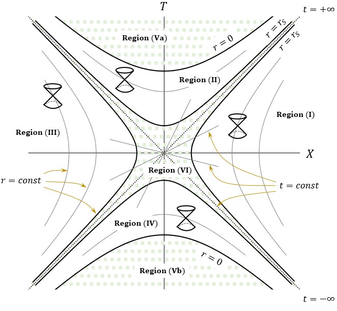
Figure 3: Kruskal-Szekeres diagram for the generalized CL metric when $A_{-}\neq 1$. The “gulf” shown as Region (VI) generally involves curvature singularity on the interior-exterior boundary.

VI.2 Key aspects of the Kruskal-Szekeres diagram of the generalized Campanelli-Lousto metric

Along the radial direction, viz. $d\theta=d\phi=0$, metric (84) is

$$ds^{2}=-4r_{\text{s}}^{2}e^{-\frac{r^{*}}{r_{\text{s}}}}\left|1-\frac{r_{\text{s}}}{r}\right|^{A_{+}+A_{-}}\left(dT^{2}-dX^{2}\right)$$ (87)

The Kruskal-Szekeres (KS) plane for metric (87) (to be called the CL–KS diagram hereafter) is illustrated in Fig. 3, which exhibits several significant characteristics, including:

• Similar to the KS diagram of the Schwarzschild metric, the CL–KS diagram is conformally Minkowski. The null geodesics are $dX=\pm dT$. Therefore, light cones align along the $45^{\circ}$ lines in the CL–KS plane.

• The CL–KS diagram essentially preserves the causal structure of the standard KS diagram, albeit with some quantitative modifications. A constant–$r$ contour corresponds to a hyperbola, while a constant–$t$ contour corresponds to a straight line running through the origin of the $(T,X)$ plane. The coordinate origin $r=0$ amounts to $T^{2}-X^{2}=1$, since $r^{*}(r=0)=0$.

• The interior-exterior boundary $r=r_{\text{s}}$ is represented by two distinct hyperbolae, one for the interior and the other for the exterior, per

  $$T^{2}-X^{2}=\begin{cases}-e^{-\frac{\pi A_{-}}{\sin\pi A_{-}}}&\text{for exterior}\\ +e^{-\frac{\pi A_{-}}{\sin\pi A_{-}}}&\text{for interior}\end{cases}$$ (88)

  It is worth noting that each hyperbola has two separate branches on its own. For $A_{-}=1$, the hyperbolae (88) degenerate into two straight lines, $T=\pm X$, as is expected for Schwarzschild black holes. In this limit, Region (VI) disappears.

• Region (I) refers to the exterior, extending up to the right branch of the hyperbola $T^{2}-X^{2}=-e^{-\frac{\pi A_{-}}{\sin\pi A_{-}}}$. Region (II) refers to the interior, extending up to the upper branch of the hyperbola $T^{2}-X^{2}=+e^{-\frac{\pi A_{-}}{\sin\pi A_{-}}}$.

• Regions (III) and (IV) are mirror images of Regions (I) and (II), upon flipping the sign of the KS coordinates, viz. $(T,X)\leftrightarrow(-T,-X)$. Regions (Va) and (Vb) are unphysical, viz. $r<0$.

• Region (VI) generally contains the curvature singularity (encoded in the Kretschmann invariant per Eq. (34)) on the interior-exterior boundary, $r=r_{\text{s}}$. The region sandwiches between the four hyperbola branches given by (88) and disappears when $A_{-}=1$.

Further discussions about the causal structure of the $\zeta-$KS diagram (for the special Buchdahl-inspired metric) have been made in Ref.  [30], and we shall not reiterate them here. These discussions are equally applicable for the present case, e.g. the CL–KS diagram, with Region (VI) being a new feature compared with the KS diagram of the Schwarzschild metric.

In summary, the CL–KS diagram represents the maximal analytic extension of the generalized CL metric. The emergence of the “gulf” in the CL–KS diagram indicates fundamental changes in the topology of spacetime around a mass source when the metric parameters deviate from their Schwarzschild value, that is when $(A_{+},A_{-})\neq(0,1)$.

VII Conclusions

Our paper took a crucial step forward by generalizing the Campanelli-Lousto (CL) solution presented in Ref.  [22], which was only valid for the exterior region. Our new generalized CL solution holds for all values of the radial coordinate $r\in R$, making it applicable to both the interior and exterior regions. Equipped with this generalization, we were able to revisit and expand upon the analysis previously produced by Agnese and La Camera [21], gaining new insights.

The generalized CL metric depends on four parameters: the Schwarzschild radius $r_{\text{s}}$, the asymptotic value of the scalar field at spatial infinity $\phi_{0}$, and the exponents $A$ and $B$ of the metric components $g_{tt}$ and $g_{rr}$, respectively. The values of $A$ and $B$ are related by the Brans-Dicke parameter $\omega$. By examining the metric on a two-dimensional plane $(A,B)$, we found that for $B$ in the range $(-\infty,-1)$, the metric supports a Morris-Thorne wormhole, while for $B$ in the range $(-1,+\infty)$, a naked singularity results. The value of $A$ has no effect on this behavior.

We further discovered that violating the Weak Energy Condition (WEC) does not necessarily lead to the formation of a wormhole. However, it does result in a divergence of the areal radius in the interior region, occurring at either $r=0$ or $r=r_{\text{s}}$. This means that WEC violation causes a change in the topology of spacetime, including in the interior region. A wormhole is formed only if the divergence takes place at $r=r_{\text{s}}$. Therefore, a wormhole is only an indirect consequence of WEC violation and a by-product of this topology change.

Finally, we established a connection between the special Buchdahl-inspired metric, that is known to be asymptotically flat for pure $\mathcal{R}^{2}$ gravity [30], and the generalized CL metric. This connection guided us to construct the maximal analytic extension of the generalized CL metric. Figure 3 depicts the Kruskal-Szekeres diagram for this metric, with Region (VI) that sandwiches between the four quadrants representing a new feature for Brans-Dicke gravity.

Overall, our findings indicate a complex interplay between the WEC violation and wormhole formation in Brans-Dicke gravity. The novel features observed in our study provide new insights into the behavior of gravity in this theory, and may have implications for modified theories of gravitation at large.

—————–$\infty$—————–

Appendix A    ON BRANS SOLUTIONS OF TYPE II, III AND IV

Although the relations among the four types of the Brans solutions have been covered in [42, 43, 44, 45], we shall reveal one more relation which has been obscure.

The Brans type IV solution can be obtained from the Brans type I solution by sending $A$ and $B$ to infinity and $r_{\text{s}}$ to zero while keeping the products $A\,r_{\text{s}}$ and $B\,r_{\text{s}}$ fixed. This can be seen as follows. When $r_{\text{s}}\rightarrow 0$, the terms $1\pm\frac{r_{\text{s}}}{4\bar{r}}$ are approximately $e^{\pm\frac{r_{\text{s}}}{4\bar{r}}}$; thus the Brans type I metric (6) and scalar field (7) respectively become

$$ds^{2} \approx-e^{-\frac{Ar_{\text{s}}}{\bar{r}}}dt^{2}+e^{-\frac{Br_{\text{s}}}{\bar{r}}}\left(d\bar{r}^{2}+\bar{r}^{2}d\Omega^{2}\right)$$ (89)

$$\phi \approx\phi_{0}\,e^{\frac{(A+B)r_{\text{s}}}{2\bar{r}}}$$ (90)

Denote $B=-(C+1)\,A$ and $r^{\prime}_{\text{s}}=A\,r_{\text{s}}$. These expressions yield

$$ds_{\text{Brans-IV}}^{2} =-e^{-\frac{r^{\prime}_{\text{s}}}{\bar{r}}}dt^{2}+e^{\frac{(C+1)r^{\prime}_{\text{s}}}{\bar{r}}}\left(d\bar{r}^{2}+\bar{r}^{2}d\Omega^{2}\right)$$ (91)

$$\phi_{\text{Brans-IV}} =\phi_{0}\,e^{-\frac{Cr^{\prime}_{\text{s}}}{2\bar{r}}}$$ (92)

which form the Brans type IV solution. For a given value of $\omega\in\mathbb{R}$, the relation in (8) reads

$$A^{2}-(C+1)A^{2}+(C+1)^{2}A^{2}-1=-\frac{\omega}{2}C^{2}A^{2}$$ (93)

With $A$ being sent to infinity, this relation yields

$$(\omega+2)C^{2}+2C+2=0$$ (94)

hence

$$C_{\pm}=\frac{-1\pm\sqrt{-(2\omega+3)}}{\omega+2}$$ (95)

The Brans type III solution is trivially the “mirror” image of Type IV by a reflection, $\frac{\bar{r}}{r^{\prime}_{\text{s}}}\leftrightarrows\frac{r^{\prime}_{\text{s}}}{\bar{r}}$ . That is

$$ds_{\text{Brans-III}}^{2} =-e^{-\frac{\bar{r}}{r^{\prime}_{\text{s}}}}dt^{2}+\frac{r_{\text{s}}^{4}}{\bar{r}^{4}}e^{\frac{(C+1)\bar{r}}{r_{{}^{\prime}\text{s}}}}\left(d\bar{r}^{2}+\bar{r}^{2}d\Omega^{2}\right)$$ (96)

$$\phi_{\text{Brans-III}} =\phi_{0}\,e^{-\frac{C\bar{r}}{2r_{s}}}$$ (97)

As was noticed in [42], the Brans type II solution is a curious case. It is a “continuation into the complex plane” by making a formal replacement in the Brans type I solution (6)–(7), per

$$r_{\text{s}}\rightarrow i\,r_{\text{s}};\ \ \ A\rightarrow i\,A;\ \ \ B\rightarrow i\,B$$ (98)

That is

$$ds_{\text{Brans-II}}^{2} =-e^{4A\arctan\frac{r_{\text{s}}}{4\bar{r}}}dt^{2}$$

$$+\left(1+\frac{r_{\text{s}}^{2}}{16\bar{r}^{2}}\right)^{2}e^{4B\arctan\frac{r_{\text{s}}}{4\bar{r}}}\left(d\bar{r}^{2}+\bar{r}^{2}d\Omega^{2}\right)$$ (99)

$$\phi_{\text{Brans-II}} =\phi_{0}\,e^{-2(A+B)\arctan\frac{r_{\text{s}}}{4\bar{r}}}$$ (100)

The relation in (8) becomes

$$\omega_{\text{Brans-II}}=-2\,\frac{A^{2}+AB+B^{2}+1}{(A+B)^{2}}\in\mathbb{R^{-}}$$ (101)

Appendix B    DIRECT VERIFICATION OF THE GENERALIZED CAMPANELLI-LOUSTO SOLUTION

In this Appendix, we shall directly check that the generalized CL metric and scalar field, given in Eqs. (19) and (20), constitute a vacuo solution to the Brans-Dicke (BD) field equations. (In addition, this exercise can also be carried out with the aid of any standard symbolic-software package, such as Mathematica or Maxima Online.)

The BD field equations in vacuo can be cast as (for $\omega\neq-3/2$)

$$G_{\mu\nu} =\frac{1}{\phi}\nabla_{\mu}\nabla_{\nu}\phi-\frac{1}{\phi}\square\,\phi+\frac{\omega}{\phi^{2}}X_{\mu\nu}$$ (102)

$$\square\,\phi =0$$ (103)

with

$$G_{\mu\nu} :=\mathcal{R}_{\text{$\mu\nu$}}-\frac{1}{2}g_{\mu\nu}\mathcal{R}$$ (104)

$$X_{\mu\nu} :=\nabla_{\mu}\phi\nabla_{\nu}\phi-\frac{1}{2}g_{\mu\nu}\nabla_{\lambda}\phi\nabla^{\lambda}\phi$$ (105)

With Eqs. (19) and (20), the Einstein tensor $G_{\mu\nu}:=\mathcal{R}_{\mu\nu}-\frac{1}{2}g_{\mu\nu}\mathcal{R}$ is

$$G_{00} =\frac{1-B^{2}}{4r^{4}}r_{\text{s}}^{2}\left|1-\frac{r_{\text{s}}}{r}\right|^{A-B-2}$$ (106)

$$G_{11} =\frac{r_{\text{s}}}{4r^{4}}\frac{(B^{2}+2AB-2(A+B)+1)r_{\text{s}}+4(A+B)r}{\left(1-\frac{r_{\text{s}}}{r}\right)^{2}}$$ (107)

$$G_{22} =\frac{r_{\text{s}}}{4r^{2}}\frac{(A^{2}+A+B-1)r_{\text{s}}-2(A+B)r}{1-\frac{r_{\text{s}}}{r}}$$ (108)

$$G_{33} =G_{22}\,\sin^{2}\theta$$ (109)

The d’Alembertian acting on a scalar field is

$$\square\phi =\frac{1}{\sqrt{-g}}\partial_{\mu}(\sqrt{-g}g^{\mu\nu}\partial_{\nu}\phi)$$ (110)

Next, we have

$$\sqrt{-g} =\left|1-\frac{r_{\text{s}}}{r}\right|^{\frac{A}{2}+\frac{3B}{2}+1}r^{2}\sin\theta$$ (111)

$$\sqrt{-g}g^{11} =\left|1-\frac{r_{\text{s}}}{r}\right|^{\frac{A}{2}+\frac{B}{2}}\left(1-\frac{r_{\text{s}}}{r}\right)r^{2}\sin\theta$$ (112)

$$\sqrt{-g}\,\square\,\phi =\partial_{r}\left(\sqrt{-g}g^{11}\partial_{r}\phi\right)$$ (113)

$$=\sin\theta\,\partial_{r}\biggl{(}\left|1-\frac{r_{\text{s}}}{r}\right|^{\frac{A}{2}+\frac{B}{2}}\left(1-\frac{r_{\text{s}}}{r}\right)r^{2}\times$$

$$\ \ \ \ \ \ \ \ \ \ \ \ \ \ \ \ \ \ \partial_{r}\biggl{(}\phi_{0}\left|1-\frac{r_{\text{s}}}{r}\right|^{-\frac{A+B}{2}}\biggr{)}\biggr{)}$$ (114)

$$=-\frac{A+B}{2}\sin\theta\,\phi_{0}\times$$

$$\partial_{r}\left(\left|1-\frac{r_{\text{s}}}{r}\right|^{-1}\left(1-\frac{r_{\text{s}}}{r}\right)\text{sgn}\left(1-\frac{r_{\text{s}}}{r}\right)\right)$$ (115)

$$=0\text{\ \ \ \ \ }\forall r$$ (116)

in which we have used $\partial_{x}\left|x\right|=\text{sgn}(x)$. For a scalar field:

$$\nabla_{\mu}\nabla_{\nu}\phi =\partial_{\mu}\partial_{\nu}\phi-\Gamma_{\mu\nu}^{\lambda}\partial_{\lambda}\phi$$ (117)

we then have

$$\nabla_{0}\nabla_{0}\phi =-\Gamma_{00}^{1}\phi^{\prime}$$ (118)

$$=\frac{\phi_{0}r_{\text{s}}^{2}}{4r^{4}}\left|1-\frac{r_{\text{s}}}{r}\right|^{\frac{A}{2}-\frac{3B}{2}-2}A(A+B)$$ (119)

$$\nabla_{1}\nabla_{1}\phi =\phi^{\prime\prime}-\Gamma_{11}^{1}\phi^{\prime}$$ (120)

$$=\frac{\phi_{0}r_{\text{s}}}{4r^{4}}\left|1-\frac{r_{\text{s}}}{r}\right|^{-\frac{A}{2}-\frac{B}{2}-2}\times$$ (121)

$$\left[(2B^{2}+3AB-2(A+B)+A^{2})r_{\text{s}}+4(A+B)r\right]$$ (122)

$$\nabla_{2}\nabla_{2}\phi =-\Gamma_{22}^{1}\phi^{\prime}$$ (123)

$$=-\frac{\phi_{0}r_{\text{s}}}{4r^{2}}\left|1-\frac{r_{\text{s}}}{r}\right|^{-\frac{A}{2}-\frac{B}{2}}\left(1-\frac{r_{\text{s}}}{r}\right)^{-1}\times$$ (124)

$$\left[(B^{2}+AB-(A+B))r_{\text{s}}+2(A+B)r\right]$$ (125)

$$\nabla_{3}\nabla_{3}\phi =\nabla_{2}\nabla_{2}\phi\,\sin^{2}\theta$$ (126)

and

$$X_{00} =-\frac{1}{2}g_{00}\left(g^{11}(\phi^{\prime})^{2}\right)$$ (127)

$$=\phi_{0}^{2}r_{\text{s}}^{2}\frac{(A+B)^{2}}{8r^{4}}\left|1-\frac{r_{\text{s}}}{r}\right|^{-2B-2}$$ (128)

$$X_{11} =(\phi^{\prime})^{2}-\frac{1}{2}g_{11}\left(g^{11}(\phi^{\prime})^{2}\right)$$ (129)

$$=\phi_{0}^{2}r_{\text{s}}^{2}\frac{(A+B)^{2}}{8r^{4}}\left|1-\frac{r_{\text{s}}}{r}\right|^{-A-B-2}$$ (130)

$$X_{22} =-\frac{1}{2}g_{22}\left(g^{11}(\phi^{\prime})^{2}\right)$$ (131)

$$=-\phi_{0}^{2}r_{\text{s}}^{2}\frac{(A+B)^{2}}{8r^{2}\left(1-\frac{r_{\text{s}}}{r}\right)}\left|1-\frac{r_{\text{s}}}{r}\right|^{-A-B}$$ (132)

$$X_{33} =X_{22}\,\sin^{2}\theta$$ (133)

From this stage, it is straightforward to verify, components by components, that the generalized CL metric and scalar field in Eqs. (19) and (20) satisfy the Brans-Dicke field equations, viz. Eq. (102) and $\square\,\phi=0$, for all $r\neq r_{\text{s}}$.

References

- [1] T. Damour and S. N. Solodukhin, Wormholes as black hole foils, Phys. Rev. D 76, 024016 (2007), arXiv:0704.2667 [gr-qc]
- [2] C. Bambi, Can the supermassive objects at the centers of galaxies be traversable wormholes? The first test of strong gravity for mm/sub-mm very long baseline interferometry facilities, Phys. Rev. D 87, 107501 (2013), arXiv:1304.5691 [gr-qc]
- [3] M. Azreg-Aïnou, Confined-exotic-matter wormholes with no gluing effects - Imaging supermassive wormholes and black holes, JCAP 07, 037 (2015), arXiv:1412.8282 [gr-qc]
- [4] V. Dzhunushaliev, V. Folomeev, B. Kleihaus, and J. Kunz, Can mixed star-plus-wormhole systems mimic black holes?, JCAP 08, 030 (2016), arXiv:1601.04124 [gr-qc]
- [5] V. Cardoso, E. Franzin, and P. Pani, Is the Gravitational-Wave Ringdown a Probe of the Event Horizon?, Phys. Rev. Lett. 116, 171101 (2016), arXiv:1602.07309 [gr-qc]
- [6] R. A. Konoplya and A. Zhidenko, Wormholes versus black holes: quasinormal ringing at early and late times, JCAP 12, 043 (2016), arXiv:1606.00517 [gr-qc]
- [7] K. K. Nandi, R. N. Izmailov, A. A. Yanbekov, and A. A. Shayakhmetov, Ring-down gravitational waves and lensing observables: How far can a wormhole mimic those of a black hole?, Phys. Rev. D 95, 104011 (2017), arXiv:1611.03479 [gr-qc]
- [8] P. Bueno, P. A. Cano, F. Goelen, T. Hertog, and B. Vercnocke, Echoes of Kerr-like wormholes, Phys. Rev. D 97, 024040 (2018), arXiv:1711.00391 [gr-qc]
- [9] J. G. Cramer, R. L. Forward, M. S. Morris, M. Visser, G. Benford, and G. A. Landis, Natural wormholes as gravitational lenses, Phys. Rev. D 51, 3117 (1995), arXiv:astro-ph/9409051
- [10] P. G. Nedkova, V. K. Tinchev, and S. S. Yazadjiev, Shadow of a rotating traversable wormhole, Phys. Rev. D 88, 124019 (2013), arXiv:1307.7647 [gr-qc]
- [11] T. Harko, Z. Kovacs, and F. S. N. Lobo, Thin accretion disks in stationary axisymmetric wormhole spacetimes, Phys. Rev. D 79, 064001 (2009), arXiv:0901.3926 [gr-qc]
- [12] E. Deligianni, J. Kunz, P. Nedkova, S. Yazadjiev, and R. Zheleva, Quasiperiodic oscillations around rotating traversable wormholes, Phys. Rev. D 104, 024048 (2021), arXiv:2103.13504 [gr-qc]
- [13] V. De Falco, M. De Laurentis, and S. Capozziello, Epicyclic frequencies in static and spherically symmetric wormhole geometries, Phys. Rev. D 104, 024053 (2021), arXiv:2106.12564 [gr-qc]
- [14] K. Jusufi, A. Övgün, A. Banerjee, and İ. Sakallı, Gravitational lensing by wormholes supported by electromagnetic, scalar, and quantum effects, Eur. Phys. J. Plus 134, 428 (2019), arXiv:1802.07680 [gr-qc]
- [15] İ. Sakallı and A. Övgün, Gravitinos tunneling from traversable Lorentzian wormholes, Astrophys Space Sci 359, 32 (2015), arXiv:1506.00599 [gr-qc]
- [16] M. S. Morris and K. S. Thorne, Wormholes in spacetime and their for interstellar travel: A tool for teaching general relativity, Am. J. Phys. 56, 5 (1988)
- [17] M. S. Morris, K. S. Thorne, and U. Yurtsever, Wormholes, Time Machines, and the Weak Energy Condition, Phys. Rev. Lett. 61, 1446 (1988)
- [18] M. Visser, Traversable wormholes from surgically modified Schwarzschild spacetimes, Nucl. Phys. B 328, 203 (1989), arXiv:0809.0927 [gr-qc]
- [19] S. Kar, Evolving wormholes and the weak energy condition, Phys. Rev. D 49, 862 (1994)
- [20] R. Shaikh and S. Kar, Wormholes, the weak energy condition, and scalar-tensor gravity, Phys. Rev. D 94, 024011 (2016), arXiv:1604.02857 [gr-qc]
- [21] A. G. Agnese and M. La Camera, Wormholes in the Brans-Dicke theory of gravitation, Phys. Rev. D 51, 2011 (1995)
- [22] M. Campanelli and C. Lousto, Are Black Holes in Brans-Dicke Theory precisely the same as in General Relativity?, Int. J. Mod. Phys. D 2, 451 (1993), arXiv:gr-qc/9301013
- [23] E-A. Kontou and K. Sanders, Energy conditions in general relativity and quantum field theory, Class. Quant. Grav. 37, 193001 (2020), arXiv:2003.01815 [gr-qc]
- [24] K. K. Nandi and A. Islam, Brans wormholes, Phys. Rev. D 55, 2497 (1997) 2497, arXiv:0906.0436 [gr-qc]
- [25] A. G. Agnese and M. La Camera, Schwarzschild metrics, quasi-universes and wormholes, in Sidharth, B.G., Altaisky, M.V. (eds) Frontiers of Fundamental Physics 4. Springer, Boston, MA, doi.org/10.1007/978-1-4615-1339-1_18, arXiv:astro-ph/0110373
- [26] J. L. Blázquez-Salcedo, C. Knoll, and E. Radu, Traversable wormholes in Einstein-Dirac-Maxwell theory, Phys. Rev. Lett. 126, 101102 (2021), arXiv:2010.07317 [gr-qc]
- [27] K. Jusufi, S. Kumar, M. Azreg-Aïnou, M. Jamil, Q. Wu, and C. Bambi, Constraining wormhole geometries using the orbit of S2 star and the Event Horizon Telescope, Eur. Phys. J. C 82, 633 (2022), arXiv:2106.08070 [gr-qc]
- [28] F. Duplessis and D. A. Easson, Exotica ex nihilo: Traversable wormholes non-singular black holes from the vacuum of quadratic gravity, Phys. Rev. D 92, 043516 (2015), arXiv:1506.00988 [gr-qc]
- [29] J. B. Dent, D. A. Easson, T. W. Kephart, and S. C. White, Stability Aspects of Wormholes in Gravity, Int. J. Mod. Phys. D 26, 1750117 (2017), arXiv:1608.00589 [gr-qc]
- [30] H. K. Nguyen, Beyond Schwarzschild-de Sitter spacetimes: II. An exact non-Schwarzschild metric in pure gravity and new anomalous properties of spacetimes, Phys. Rev. D 107, 104008 (2023), arXiv:2211.03542 [gr-qc]
- [31] H. K. Nguyen, Beyond Schwarzschild-de Sitter spacetimes: I. A new exhaustive class of metrics inspired by Buchdahl for pure gravity in a compact form, Phys. Rev. D 106, 104004 (2022), arXiv:2211.01769 [gr-qc]
- [32] H. A. Buchdahl, On the Gravitational Field Equations Arising from the Square of the Gaussian Curvature, Nuovo Cimento 23, 141 (1962), link.springer.com/article/10.1007/BF02733549
- [33] H. K. Nguyen and M. Azreg-Aïnou, Traversable Morris-Thorne-Buchdahl wormholes in quadratic gravity, arXiv:2305.04321 [gr-qc]
- [34] C. H. Brans and R. Dicke, Mach’s Principle and a Relativistic Theory of Gravitation, Phys. Rev. 124, 925 (1961)
- [35] C. H. Brans, Mach’s Principle and a relativistic theory of gravitation II, Phys. Rev. 125, 2194 (1962)
- [36] L. Vanzo, S. Zerbini, and V. Faraoni, Campanelli-Lousto and veiled spacetimes, Phys. Rev. D 86, 084031 (2012), arXiv:1208.2513 [gr-qc]
- [37] K. A. Bronnikov, C. P. Constantinidis, R. L. Evangelista, and J. C. Fabris, Cold black holes in scalar-tensor theories, arXiv:gr-qc/9710092
- [38] A. S. Eddington, A Comparison of Whitehead’s and Einstein’s Formulï¿œ, Nature (London) 113, 192 (1924).
- [39] D. Finkelstein, Past-Future Asymmetry of the Gravitational Field of a Point Particle, Phys. Rev. 110, 965 (1958)
- [40] M. D. Kruskal, Maximal Extension of Schwarzschild Metric, Phys. Rev. 119, 1743 (1960)
- [41] P. Szekeres, On the Singularities of a Riemannian Manifold, Publicationes Mathematicae Debrecen 7, 285 (1960)
- [42] K. Sarkar and A. Bhadra, Strong field gravitational lensing in the Brans-Dicke theory, Class. Quant. Grav. 23 (2006) 6101, arXiv:gr-qc/0602087 [gr-qc]
- [43] V. Faraoni, F. Hammad, and S. D. Belknap-Keet, Revisiting the Brans solutions of scalar-tensor gravity, Phys. Rev. D 94, 104019 (2016), arXiv:1609.02783 [gr-qc]
- [44] V. Faraoni, F. Hammad, A. M. Cardini, and T. Gobeil, Revisiting the analogue of the Jebsen-Birkhoff theorem in Brans-Dicke gravity, Phys. Rev. D 97, 084033 (2018), arXiv:1801.00804 [gr-qc]
- [45] K. A. Bronnikov, Scalar-tensor theory and scalar charge, Acta Phys. Polon. B 4, 251 (1973)