Proper Interpretation of Heaps’ and Zipf’s Laws

Abstract

We checked that the distribution of words in text should uniform, which gives Heaps’ law as natural result, that is, the number of types of words can be expressed as a power law of the number of tokens within text. We developed a “superposition” model, which leads to an asymptotic power-law distribution of the number of occurrences (or frequency) of words, that is, Zipf’s law. The model is well consistent with observations.

keywords:

Zipf’s law; Heaps’ law; arithmetic growth; power-law distribution

Zipf’s law of words frequency in text is a most typical example of the power-law distribution. Zipf’s law has been reported in various phenomena including economic, astrophysical and so on and its mechanisms have been developed diversely. Most authors believed and tried to explain those phenomena by a unique mechanism. However, I would claim that different phenomena occur from different causes so that Zipf’s law in language process is based on an arithmetic growth of words while other phenomena can be caused by a geometric growth. It has been pursued to develop a mechanism proper to language process and stable, though neither omnipotent nor with delicate manipulation.

1 Introduction

The distribution of words in language process such as text or speech is a problem difficult to study only in statistical way. Despite table experiment is possible or even we can trace one by one word in text, its mechanism is being under the discussion. The distribution of words seems to have no a centrality, but a skewness. This distribution is attributed to a power-law distribution called Zipf’s law.

The power-law distribution has already been studied for more than a century. Estoup (1916) and Zipf (1932) found that the distribution in word frequency in novel is a power-law one, i.e. the number of types of words is reciprocal to their number of occurrences. Many phenomena in economics and astrophysics and so on have been found to follow the power-law distribution (e.g. see Newman, 2005). Most of them had been attributed to Zipf’s law, despite Zipf’s law is originally related to the word distribution.

Several generative models have been proposed to explain the power-law distribution including Zipf’s law for word frequency. One of the most famous models is the “preferential attachment” process (Yule, 1924; Simon, 1955; Barabasi & Albert, 1999). Originally, this model had been developed for the distribution of size of biological genera or species. However, such systems give a geometric growth while the number of words in text increases arithmetically. Furthermore, the original “preferential attachment” model assumed the rate of new words as constant along text (e.g. see Li, 2016), which is inconsistent with the observation as to text, in particular Heaps’ law (Heaps, 1978) that says that the rate of new words decreases along text. Though the model can be modified so that this rate varies along text, the rule of manipulation to choose words in the process is not verified in practice.

A competitive model might be “principle of least effort” or an optimization model. This model was originally by Estoup (1916) and Zipf (1936, 1949) and developed by Mandelbrot (1953) and recent workers (e.g. see Ferrer i Cancho & Solé, 2003). However, the model seems less intuitive and casts a suspicion to people. In fact, it is similar to the principle of least action in physics, which, however, has a unique solution while text, though of the same content, can vary from person to person, from language to language or even from time to time by a single person. Additionally speaking, Zipf’s law is detected in all the languages including even those that have not articles or prepositions as in English (Yu et al., 2018). Zipf’s law has been reported to appear in children’s utterance or schizophrenic speech (Zipf, 1942; Piotrovskii, Pashkovskii & Piotrovskii, 2012; Alexander, Johnson & Weiss, 1998), for which I am afraid if they try to optimize their speaking. Williams et al. (2015) showed Zipf’s law for clauses, phrases, words and even for graphemes and letters.

Another important model is “Monkey’s typing randomly” or “intermittent silence” that was proposed by Miller (1957) and studied recently (e.g. see Li, 1992). In this model, a sequence of randomly selected character turns out to be a word, if it is separated by blank spaces inserted randomly as well. It has been shown that the word of randomly generated characters has a power-law distribution similar to Zipf’s law. The model seems to be based only on a blind statistical consideration without sophisticated manipulation. However, the power-law distribution is originated from a morphological trend that “short words” are more frequent but less abundant than “long words”. That trend is in turn originated only from the way of making word from characters in the model but cannot be reproduced in real text.

A graphical analysis also has been studied, which, however, seems more complex but less effective (e.g. see Natale, 2018). Other manipulative or artificial processes such as SSR process (Corominas-Murtra, 2015) or Pólya’s urn model (Pólya, 1930) were studied, but it is not confident if those processes could represent the language process properly. The distribution might be broken if an item of those manipulations would be changed. According to the previous works, Zipf’s law seems so pertinacious or sticky that arbitrary text or speech include the law.

As aforementioned, the power-law distribution has also been found in economic phenomena such as income taxes (Pareto, 1896), the population in city (Auerbach, 1913; Zipf, 1949) or firm size distribution (Axtell, 2001). Based on Gibrat’s model (Gibrat, 1931), Gabaix (1999) gave an explanation of Zipf’s law for population in city. Chol-jun (2022) developed a model called “geometrically growing system” that can explain the power-law distribution appeared in broad fields such as demography, epidemiology or econometrics. However, those models seem to have no relevance to glottometrics. In fact, the increase of the word occurrences along text seems arithmetic but not geometric.

To summarize, all the aforementioned models seem to be improper to language process.

2 Phenomenological Analysis of Language Process

In order to make a proper interpretation of Heaps’ or Zipf’s laws, we need to analyze real language process such as text or speech. We have analyzed texts and could pick some properties.

The number of frequent words, including grammatical words such as “the” or “could” and keywords of content, increases linearly along with the length of text. Of course, we cannot verify this rule for very rare words or hapax legomena because they appear only one or two times in text. Meanwhile, the words of a given number of occurrences are distributed uniformly throughout text, which suggests a uniform distribution of words.

Some words appear relatively intensively in some places of text, i.e. intermittently. Typically, keywords of a paragraph or a chapter appear intensively in relevant paragraphs or chapters. Some grammatical words depending on context such as “have” or “could” also show such a “local grouping”. This makes the global analysis of the word distribution more difficult.

Zipf’s law appears not only in long text or corpora, but also in short text which includes a few paragraphs or even in list composed of incomplete sentences such as titles. This lets us consider Zipf’s law as a pertinacious or internal property of language process. However, “internal” should not imply “axiomatic.” There is no “absolute” frequency of the words except a few grammatical words such as “the.” In other words, the frequency of a word is varying from text to text, probably depending on the content or context.

Among the parts of sentences, the frequency lowers from the subject to the object, then to the adverbial, and at last to the predicate, neglecting the attributive as independent part. In fact, the hero of a novel has most frequency and the story is woven with various actions of him. A clear point of Zipf’s or Mandelbrot’s optimization model is a trend to maximize the information in language process. During inspection, we can be sure that almost words in text never repeat except a few words. But those a few words show Zipf’s law, where even non-iterative words are involved so that extending power-law distribution to the number of occurrences 1 or 2. The verbs or the adjectives as the predicative have the main responsibility of such a maximization of information.

Zipf’s law between the frequency or the number of occurrences (hereafter, the occurrences in short) and its rank leads to another power-law distribution for the probability of the occurrences. When drawing the histogram of the occurrences (e.g. see Fig. 4), a power-law distribution is obvious, in particular for rare words, while the distribution is discreet for high occurrences.

A correlation between the content of sentences affects the slope of Zipf’s law or Heaps exponent. As we took experiment with lists of titles, if the titles are of the same field, which implies a greater correlation between them, then Heaps’ exponent and the slope in histogram for the occurrences, in particular for rare words, lower. If the titles are of less correlative themes, Heaps exponent tends to unity, i.e. there appears almost only new words along text, and the slope in the histogram increases, seeming, however, to keep the approximate power law itself for rare words.

Among the aforementioned statistical and lexicological properties, we try to identify only one property: the word appearance follows a uniform distribution. This property is obvious for frequent words such as “the”, but difficult to check for rare words or hapax legomena, as aforementioned. If a word appears with the uniform distribution, its number of occurrences follows Poisson distribution. In fact, the uniform and Poisson distributions are both sides of the same coin: if the word appears in uniform distribution, its first position in text or the span $x$ between its replicas should follow a distribution derived from Poisson distribution (e.g. see Feller, 1971): $p(x)=\lambda\exp(-\lambda x)$. Here $\lambda$ stands for the probability of occurrence of the word and is defined as $\lambda=\frac{k}{X}$, where $k$ stands for the occurrences of the word and $X$ for the length of text or the number of tokens (hereafter, shortly the tokens). We can estimate the mean of $x$ as $\bar{x}=\int_{0}^{\infty}x\lambda\exp(-\lambda x)dx=\frac{1}{\lambda}$. Therefore, we could expect an inverse relation between the occurrences $k$ and the mean first position $\bar{x}$ of the words of the same $k$, i.e. that of all the words appeared $k$ times in text, if the words are supposed to appear uniformly:

$$\bar{x}=\frac{X}{k}.$$ (1)

.

Figure 1 shows that the above inverse relation holds all over the occurrences approximately. Therefore, we can apply the assumption of the uniform distribution not only to frequent words but also to the rarest words that appear only one time in the corpus. As a resource text throughout this paper, author’s debut paper Chol-jun (2019) is analyzed, which might be in broken English so that could be a kind of challenge to Zipf’s law found in normal or proper English libraries.

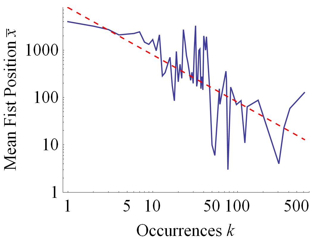
Figure 1: The relation of the number of occurrences of word $k$ vs. the mean first positions $\bar{x}$ for the words of the same $k$. The red dashed line implies $\bar{x}=\frac{X}{k}$, which has the slope of $-1$. This relation seems coincident with data throughout all the occurrences.

3 Derivation of Heaps’ law

Most authors derived Heaps’ law from Zipf’s law (e.g. see Bernhardsson, Baek & Minnhagen, 2011; Boytsov, 2017; van Leijenhorst, 2005; Lü, Zhang & Zhou, 2016), adopting Zipf’s law as an axiomatic property of language process without proof. However, as Zipf’s law seems more subtle and less intuitive than Heaps’ law, a reverse derivation seems more desirable. Deriving Heaps’ law, the previous workers take the mean span of words as a first position of them, but such an assumption is clearly improper. The first position is no more than an instance of the span, but cannot represent the mean span.

We can intuitively expect that the rate of new words should be lowering along text because the number of already appeared words is growing and they all continue to appear in later part of text. Assuming that the word appearance follows a uniform distribution, let’s formulate this process. Let $x$ stand for the position of word within text, $X$ for the whole length or the number of tokens (hereafter, simply the tokens) of the text, $y$ for the number of types (hereafter, simply the types) of words appeared from the start of text to $x$ and $Y$ for the whole types of words within the text. A function $x(y)$ represents Heaps’ law itself or, as aforementioned, the first position $x$ of a word as a function of the number of types $y$ for the word. Figure 2 shows Heaps’ law with best-fit parameters for Chol-jun (2019) as resource. Despite local undulation, the overall trend justifies Heaps’ law $y=Kx^{\beta}$ with $K=2.97$ and $\beta=0.81$.

If the length of text increases by $dx$, this increment is composed of $dy$ new words and replicas of already appeared words. We can represent the mean span $\bar{x}(y)$ of a word of type $y$ as the first position of the word $x(y)$ divided by a random variable $\omega(y)$: $\bar{x}(y)=\frac{x(y)}{\omega(y)}$. The occurrences of the word $y$ within $dx$ is expected as $\frac{dx}{\bar{x}(y)}$. We can integrate such occurrences of words not from $y=1$, i.e. the start of text, but from $y=y_{i}$ to given $y$, where $y_{i}$ is a position whence Heaps’ law seems to hold. In fact, the law does not hold from the start of text.

To summarize, we can establish the following equation:

$$\frac{dy}{dx} =1-\sum_{y=y_{i}}^{y}\frac{1}{\bar{x}(y)}$$ (2)

$$\approx 1-\int_{y_{i}}^{y}\frac{dy}{\bar{x}(y)}=1-\int_{y_{i}}^{y}\frac{\omega(y)dy}{x(y)}=1-\bar{\omega}(y)\int_{y_{i}}^{y}\frac{dy}{x(y)}$$ (3)

$$=1-\bar{\omega}\int_{y_{i}}^{y}\frac{dy}{x(y)},$$ (4)

where in the fourth equation $\omega(y)$ is extracted outside of integral into a variable $\bar{\omega}(y)$ that also should be a function of $y$. In Eq. (4) we approximate $\bar{\omega}(y)$ simply by a constant $\bar{\omega}$. The fact that $\bar{\omega}(y)$ varies slowly along with $y$ will be shown by experiment later (see below Eq. 9). Eq. (4) is a simple kind of integro-differential equation.

It can be easily shown that the Heaps’ law $y=Kx^{\beta}$ is a solution of eq. (4) (see Appendix A), if relating the macroscopic quantities $K,\,\beta$ and the microscopic ones $y_{i},\,\bar{\omega}$ as follows:

$$\bar{\omega} =1-\beta,$$ (5)

$$\beta =1-\bar{\omega},$$ (6)

$$y_{i} =\left(K\beta^{\beta}\right)^{\frac{1}{1-\beta}},$$ (7)

$$K =\frac{y_{i}^{\bar{\omega}}}{(1-\bar{\omega})^{(1-\bar{\omega})}},.$$ (8)

Here are given two expressions for $\bar{\omega}$: one is macroscopic (Eq. 5), while another is microscopic, derived from Eq. (1) and  (2):

$$\bar{\omega}(y)=\frac{\sum_{y=y_{i}}^{y}\frac{1}{\bar{x}(y)}}{\sum_{y=y_{i}}^{y}\frac{1}{x(y)}}=\frac{\sum_{y=y_{i}}^{y}\frac{k(y)}{X}}{\sum_{y=y_{i}}^{y}\frac{1}{x(y)}}$$ (9)

Substituting $y_{i}$ from Eq. (7), we can compare both expressions, which is shown in Fig. 2. The $\bar{\omega}$ (Eq. 5) is evaluated piecewisely from $\beta$ best-fitted to Heaps diagram. In other words, we divided Heaps diagram into segments and inferred $\beta$ in every segment. Figure 2 shows that both expressions are consistent. We can find that $\bar{\omega}$ increases slowly along text. This corroborates two facts: the assumption of constancy of $\bar{\omega}$ and a decrement of Heaps exponent $\beta$, approaching to the end of text. The constancy can be explained by that great $y$s contribute negligibly in Eq. 2. The decrement of $\beta$ is reported by previous authors. Bernhardsson, Baek & Minnhagen (2011) announced that $\beta$ tends from $1$ for $y=1$ to $0$ as $y\rightarrow\infty$. The decrement of $\beta$ can be interpreted by that the ratio $\frac{x(y)}{\bar{x}(y)}$ could increase slowly with $y$, which in turn can be supposed by aforementioned “local grouping” or “intermittency”. For example, considering that a new hero appears at the end of a novel, he might appear relatively often in the last context, which means low ${\bar{x}(y)}$ despite the late advent, which means high first position $x(y)$.

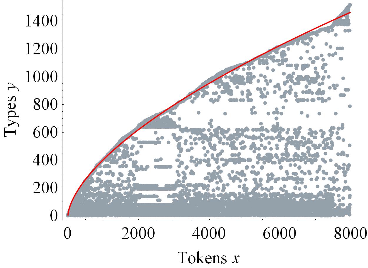
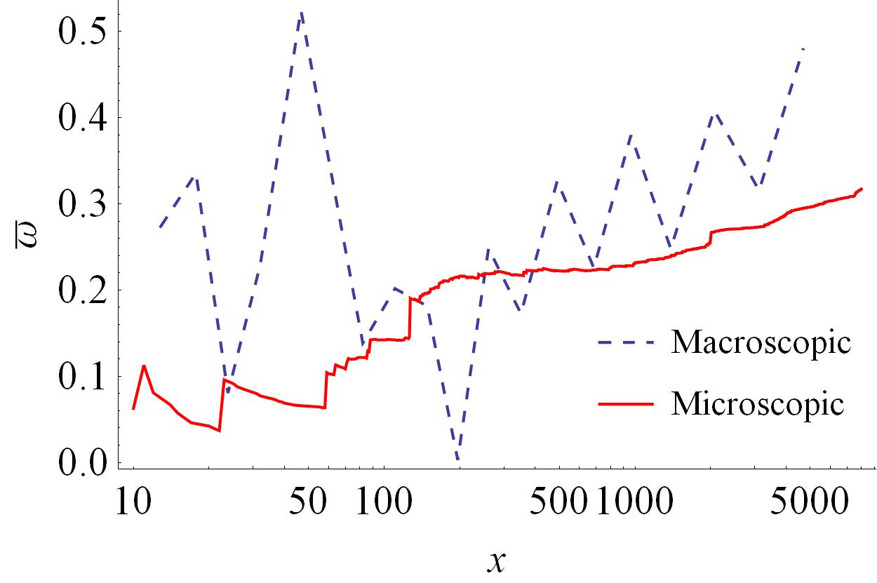
Figure 2: (a) Heaps diagram. The abscissa $x$ stands for the position in text while the ordinate $y$ for the number of type of word. The dots imply what type of word appears in what position in text. The red curve shows Heaps’ law with the best-fit parameters. The resource text is Chol-jun (2019). Though in the first part (Introduction) and the last part (References) the slope jumps due to many new words, Heaps’ law approximates overall trend of word increase well. (b) Variation of $\bar{\omega}$ vs. $x$. $\bar{\omega}$ is evaluated in both ways: macroscopic (Eq. 5) and microscopic (Eq. 9), where the macroscopic value is evaluated respectively in segments separating the whole text length equally in log-scale. The position $x$ is evaluated by Heaps’ law $y=Kx^{\beta}$. The both evaluations are excellently consistent.

It should be noted that in the model with Eq. (2) a best-fitted $y_{i}$ is obtained approximately $10\sim 15$. Heaps exponent $\beta$ is almost unity before $y=y_{i}$. This value of $y_{i}$ is almost equal to the mean span of “the” in common English text. The assumption of uniform distribution can be applied after appearance of first “the” for English text, whence Heaps’ law can be considered to hold as well. In addition, a typical value of $K$ is $2\sim 7$ and that of $\beta$ is $0.6\sim 0.8$.

4 Derivation of Zipf’s law

Here we focus on the probability density function (PDF) of the occurrences $p(k)$. Then the rank of the occurrences $r(k)$ as a function of occurrences $k$ can be defined as

$$r(k)=Y\int_{k}^{\infty}p(k)dk,$$ (10)

where $Y$ is the whole types of words in text. Then Zipf’s law implies $k(r)\sim r^{-\alpha}$.

Zipf’s law can lead to another power-law relation $p(k)\sim k^{-A}$ for $p(k)$, for which it can easily be shown that $\alpha$ and $A$ are related as

$$A=\frac{1}{\alpha}+1.$$ (11)

.

Zipf’s law also announced that $\alpha\approx 1$ in common English text. But many authors (e.g. see Bernhardsson, Baek & Minnhagen, 2011; Boytsov, 2017; van Leijenhorst, 2005; Lü, Zhang & Zhou, 2016) derived that Zipf’s exponent $\alpha$ has a relation with Heaps exponent $\beta$ as

$$\alpha=\frac{1}{\beta}.$$ (12)

However, experiments mentioned in Sec. 2 showed that for rare words, i.e. for low $k$s, $A$ increases with $\beta$ rapidly, even sometimes crossing over $2$, which is at odds with Eqs. (11) and (12) where always $\beta<1$.

The difference of $\alpha$ or $A$ between for rare words and frequent words can be shown in a simple algebraic model, where the first position of word $x(y)$ takes a part of the mean span $\bar{x}(y)$ (see Appendix B). In this model $\alpha$ and $A$ can be approximated as follows:

$$\alpha_{\text{alg}}=\left\{\begin{aligned} \frac{(X-Y+1)-\beta}{(X-Y+1)\beta}\approx\frac{1}{\beta},&\quad y\rightarrow 1\,\text{ or }\,k\rightarrow\infty\\ \frac{1}{\beta}-\frac{Y}{X},&\quad y\rightarrow Y\,\text{ or }\,k\rightarrow 1\end{aligned}\right.$$ (13)

$$A_{\text{alg}}=1+\frac{1}{\alpha_{\text{alg}}}=\left\{\begin{aligned} 1+\frac{(X-Y+1)\beta}{(X-Y+1)-\beta}\approx 1+\beta,\quad&y\rightarrow 1\,\text{ or }\,k\rightarrow\infty\\ 1+\frac{1}{\frac{1}{\beta}-\frac{Y}{X}},\quad&y\rightarrow Y\,\text{ or }\,k\rightarrow 1\end{aligned}\right..$$ (14)

In those expressions we can notify the difference of the exponents for frequent ($k\rightarrow\infty$) and rare ($k\rightarrow 1$) words. However, in this approach, $\bar{x}(y)$ is replaced with $x(y)$ and the rank $r$ is approximated by the type number $y$, which are implausible in practice.

In fact, we can derive several asymptotic power-law distributions, simulating the language process. For example, the occurrences can be expressed as the ratio between a scope of word, which means the range of the word from its first position to last position, and the mean span of word: $k(y)=\frac{l(y)}{\bar{x}(y)},$ where $k,l,\text{ and }\bar{x}$ stand for the occurrences, scope and mean span of word of type $y$, respectively. Similarly to the approach in Chol-jun (2022), we can assume that the distributions of the scope $l$ and the mean span $\bar{x}$ as normal distributions $N(\mu_{2},\sigma_{2})$ and $N(\mu_{1},\sigma_{1})$ respectively. Then, it is easy to derive the PDF of $k$.

$$p_{\text{n2n}}(k)=\frac{\sigma_{1}\sigma_{2}\exp{\left(-\frac{\mu_{1}^{2}}{2\sigma_{1}^{2}}-\frac{\mu_{2}^{2}}{2\sigma_{2}^{2}}\right)}}{\pi\left(\sigma_{1}^{2}k^{2}+\sigma_{2}^{2}\right)}+\frac{\exp{\left(-\frac{(\mu_{2}-\mu_{1}k)^{2}}{2\left(\sigma_{1}^{2}k^{2}+\sigma_{2}^{2}\right)}\right)}\left(\mu_{1}\sigma_{2}^{2}+\mu_{2}\sigma_{1}^{2}k\right)}{\sqrt{2\pi}\left(\sigma_{1}^{2}k^{2}+\sigma_{2}^{2}\right)^{\frac{3}{2}}}\text{erf}\left(\frac{\mu_{1}\sigma_{2}^{2}+\mu_{2}\sigma_{1}^{2}k}{\sqrt{2}\sigma_{1}^{2}\sigma_{2}^{2}\sqrt{\frac{1}{\sigma_{1}^{2}}+\frac{k^{2}}{\sigma_{2}^{2}}}}\right)$$ (15)

This distribution of the occurrences is an asymptotic power-law one even with exponent $-2$. This seems to explain why Zipf’s exponent is almost unity in common texts. However, this approach does not explain the dependency of Zipf’s exponent on Heaps exponent. And the real distributions of the scope and the mean span of words are deviated from the normal. Some distributions assumed for the scope and the mean span also can give the asymptotic power-law distribution of $p(k)$, though the slope can be different from -2. The practical distributions for the scope and the mean span are similar to the exponential ones probably due to the uniformity of word appearance (see Sec. 2). However, because of the exponent greater than -1 (lower than unity in absolute value) for those exponential distributions, the analytic treatment is impossible. It is another disadvantage that the scope or the mean span can be evaluated only for words appeared more than 2 times.

Now we propose a “superposition” model. Though we did not describe in Sec. 2, the length of sentences or clauses has a centralized distribution. We call the elementary unit of text a “leaf,” which could be a sentence or clause. We suppose that all the leaves have the same size, i.e. the mean size, and that all the words in a leaf are non-iterative within the leaf. The main idea is that, though a leaf is flat, a heap of leaves is not flat. The area of a leaf implies the number of words in the sentence or clause and the superposition of leaves implies the repetition of words between sentences and clauses. If a superposition between leaves occurs, the whole area of the ground covered by leaves, which means the whole types of words in text, does not increase linearly along with the number of leaves or the total area of respective leaves, which means the whole tokens in text.

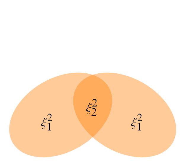
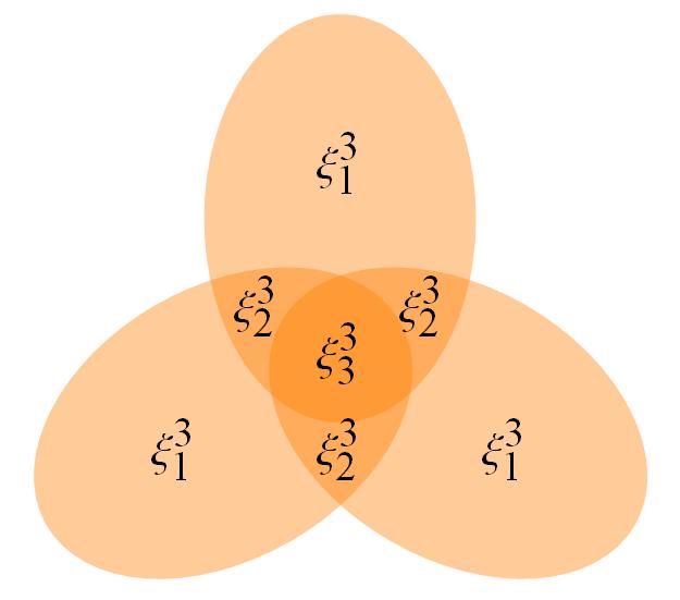
Figure 3: The superposition of leaves. $\xi^{n}_{k}$ stands for the size of a part overlaid $k$ times by $n$ leaves. Such a part has $\binom{n}{k}$ replicas.

The area of every leaf is denoted by $d$, which will be canceled out later so that it is not important. Let $n$ express the number of leaves, i.e. $n=\frac{X}{d}$. Then Heaps’ law $y=Kx^{\beta}$ can be transformed into $y=dn^{\beta}$ via $K=d^{(1-\beta)}$. If $n$ leaves are overlapped, a $k$-fold overlaid part or its area can be denoted by $\xi^{n}_{k}$. Figure 3 shows that such a part has altogether $\binom{n}{k}$ replicas. Therefore, all the types (or the number) of $k$-times appeared words is equal to $Y_{k}=\binom{n}{k}\xi^{n}_{k}$, where $Y=\sum_{k=1}^{n}Y_{k}=\sum_{k=1}^{n}\binom{n}{k}\xi^{n}_{k}$ is the total area covered by leaves or the whole types of words in text. In Fig. 3 it can easily be known that

$$\xi^{n-1}_{k-1}=\xi^{n}_{k-1}+\xi^{n}_{k},$$ (16)

which is a key formula to relate the different occurrences. As we know, the types of words, i.e. Heaps’ law, affect the occurrences distribution or Zipf’s law. Adopting Heaps’ law, we obtain $\xi^{n}_{1}=d\left(n^{\beta}-(n-1)^{\beta}\right)$ from Fig. 3. According to the above recursive relation,

$$\xi^{n}_{k}=\xi^{n-1}_{k-1}-\xi^{n}_{k-1}=d\sum_{j=0}^{k-1}(-1)^{j+k-1}\binom{k-1}{j}\left((n-j)^{\beta}-(n-j-1)^{\beta}\right).$$ (17)

It should be noted that $Y_{k}\rightarrow\infty$ for $n\rightarrow\infty$. The quantity of interest is not $Y_{k}$s, but the ratio $\frac{Y_{k}}{Y_{1}}$,i.e. the probability of the occurrences, which we evaluate now. From the above equations, we obtain

$$\frac{Y_{k}}{Y_{1}}=\frac{\binom{n}{k}\sum_{j=0}^{k-1}(-1)^{j+k-1}\binom{k-1}{j}\left((n-j)^{\beta}-(n-j-1)^{\beta}\right)}{n\left(n^{\beta}-(n-1)^{\beta}\right)},$$ (18)

which can be factorized for convenience as follows:

$$\frac{Y_{k}}{Y_{1}}=\frac{\binom{n}{k}}{n^{k}}\frac{n^{k-1}\sum_{j=0}^{k-1}(-1)^{j+k-1}\binom{k-1}{j}\left((n-j)^{\beta}-(n-j-1)^{\beta}\right)}{\left(n^{\beta}-(n-1)^{\beta}\right)},$$ (19)

Let’s consider the limit for $n\rightarrow\infty$, which can be true for almost texts. Then, the first term tends as

$$\lim_{n\rightarrow\infty}\frac{1}{n^{k}}\binom{n}{k}=\frac{1}{k!}.$$ (20)

Changing $n$ into a new variable $t=\frac{1}{n}$, the limit $n\rightarrow\infty$ can be replaced with $t\rightarrow 0$. Then we expand the ratio $\frac{(1-jt)^{\beta}-(1-(j+1)t)^{\beta}}{\left(1-(1-t)^{\beta}\right)}$ into Taylor series with respect to $t$. Taking into account that $\sum_{j=0}^{k-1}(-1)^{j+k-1}\binom{k-1}{j}j^{\eta}=0$ if $\eta<k-1$, the second term in Eq. (19) can be calculated as

$$\frac{\sum_{j=0}^{k-1}(-1)^{j+k-1}\binom{k-1}{j}\left((1-jt)^{\beta}-(1-(j+1)t)^{\beta}\right)}{t^{k-1}\left(1-(1-t)^{\beta}\right)}=\prod_{j=1}^{k-1}(j-\beta).$$ (21)

For example of $\beta=\frac{1}{2}$, the above formula gives $(-1)^{k-1}\frac{(2k-3)!!}{2^{k-1}}$. Eventually, we obtain the ratio as

$$\frac{Y_{k}}{Y_{1}}=\frac{\prod_{j=1}^{k-1}(j-\beta)}{k!},$$ (22)

which is the probability of discrete occurrences $k$.

Considering $\sum_{k=1}^{\infty}\frac{Y_{k}}{Y_{1}}=\frac{1}{\beta}$ and $\prod_{j=1}^{k-1}(j-\beta)=\frac{\Gamma(k-\beta)}{\Gamma(1-\beta)}$, we can obtain the probability or PDF of the occurrences in a continuous version of Eq. (22):

$$p_{\text{YS}}(k)=\frac{\beta\Gamma(k-\beta)}{\Gamma(k+1)\Gamma(1-\beta)},$$ (23)

which I will call YongSun distribution. Evaluate the asymptotic log-log slope of YongSun function:

$$A_{\text{YS}}=-\frac{d(\log p_{\text{YS}}(k))}{d(\log k)}=\left\{\begin{aligned} &1+\beta,\quad&k\rightarrow\infty\\ &1-\gamma-\left.\frac{\Gamma^{\prime}(z)}{\Gamma(z)}\right|_{z=1-\beta},\quad&k\rightarrow 1\end{aligned}\right.,$$ (24)

where $\gamma\approx 0.577216$ is the constant called Euler’s gamma. From Eq. (11) Zipf’s exponent can be evaluated:

$$\alpha_{\text{YS}}=-\frac{d(\log k(r))}{d(\log r)}=\left\{\begin{aligned} &\frac{1}{\beta},\quad&k\rightarrow\infty\\ &\frac{1}{-\gamma-\left.\frac{\Gamma^{\prime}(z)}{\Gamma(z)}\right|_{z=1-\beta}},\quad&k\rightarrow 1\end{aligned}\right..$$ (25)

As we can see, the exponents $\alpha$ and $A$ for frequent ($k\rightarrow\infty$) words are coincident with previous results. Note that $\left.\frac{\Gamma^{\prime}(z)}{\Gamma(z)}\right|_{z=1-\beta}$ is negative so that $\alpha_{\text{YS}}$ for $k\rightarrow 1$ is positive. The latter decreases monotonically with $\beta$ so that, when $\beta$ lowers in later part of text or Heaps diagram, Zipf’s exponent $\alpha$ for $k\rightarrow 1$ increases.

In this model, we suppose that the area of all the leaves are equal and their superposition are also equal. Hence, the uniformity of word appearance found in Sec. 2 keeps.

Figure 4 shows that the “superposition of leaves” model fits well data both in Zipf’s and $p(k)$ diagrams. For the normalization, we evaluate the rank in Fig. 4 not by Eq. (10) but by

$$r(k)=Y\int_{k}^{k_{\text{max}}}p_{\text{YS}}(k)dk+1$$ (26)

because this definition can give $r\rightarrow 1$ for $k\rightarrow k_{\text{max}}$ and $r\rightarrow Y$ for $k\rightarrow 1$, where $k_{\text{max}}$ is the maximum occurrences among the words appeared in the text. We can find that Zipf’s diagram in Fig. 4 consists of 3 segments with different slopes, which is coincident with previous works (Yu et al., 2018; Natale, 2018). However, they showed that Zipf’s exponent (in absolute value) increases for rare words of rank greater than $\sim 10^{4}$. This can be explained by that the previous workers studied the corpora or very long texts while in this paper merely a short text is considered so that Heaps’ exponent can be constant. In fact, most novels contain $10^{4}$ or $10^{6}$ words . We can think that those words are common for most novels. Therefore, in a corpus, which can be considered to be consisted of the novels, the rare words of rank greater than $10^{4}$ are contained less, which implies that Heaps exponent $\beta$ lowers for $y>10^{4}$ and, from Eq. (25), Zipf’s exponent $\alpha$ in the corpus could increase for rank greater than $\sim 10^{4}$.

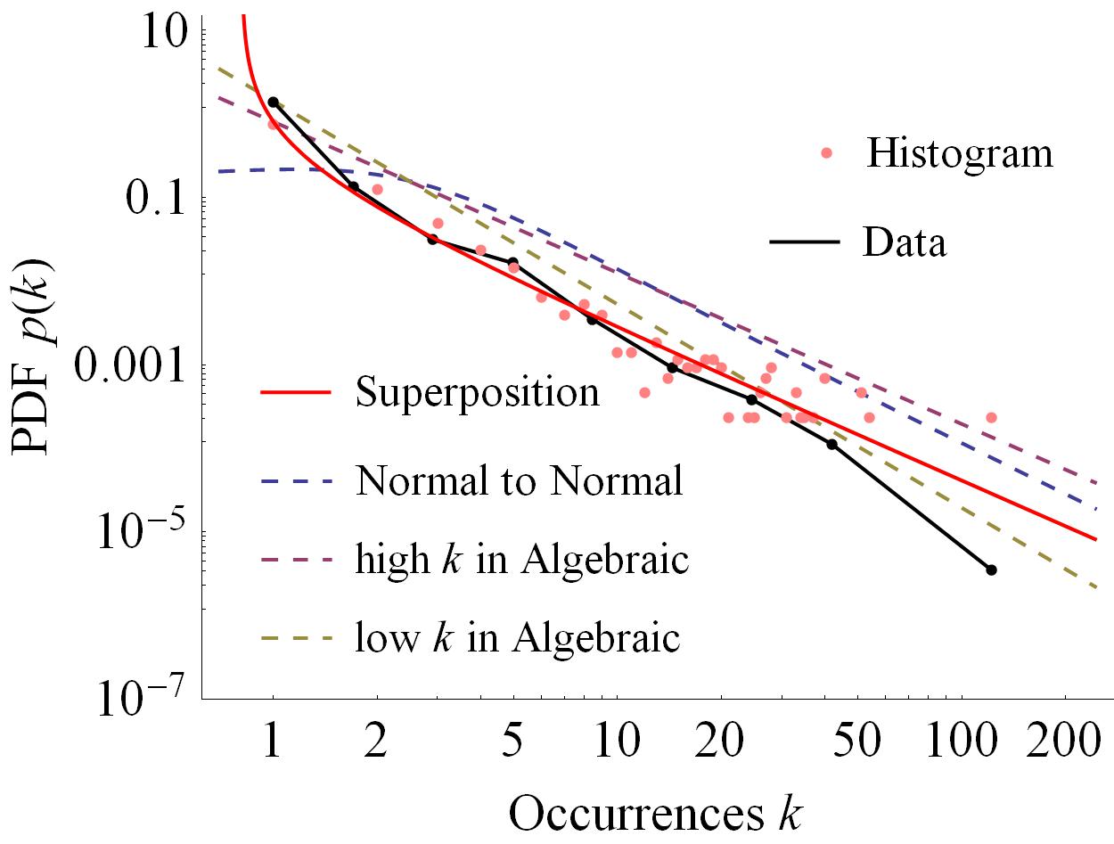
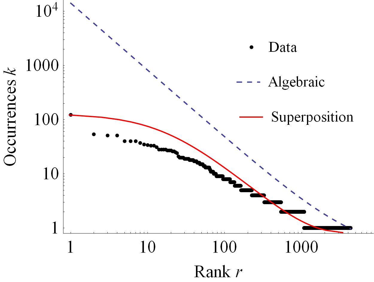
Figure 4: The comparison between data and models. The data is extracted with 2-gram model from the article Chol-jun (2019) in order to show the differences between rare and frequent words more obviously. (a) The PDF of the occurrences $k$ is evaluated by the data, the “ratio of normal to normal” (Eq. 15), algebraic and “superposition” models (Eq. 23). For the algebraic model, only the slopes evaluated in high and low occurrences limits (Eq. 14) are shown. The pink dots are drawn from the histogram of the occurrences, divided by the whole types of words $Y$. (b) Zipf’s diagram, i.e. the diagram of the occurrences $k$ vs. its rank $r(k)$. This diagram is evaluated by data, algebraic (Eq. 13) and “superposition” models. Both diagrams show that the “superposition” model fits well data.

5 Conclusion

As we have seen, words in text seem to occur with uniform distribution so that Heaps’ law can be obtained naturally. We proposed a “superposition” model and derived a YongSun distribution of the occurrences of words, which is a kind of asymptotic power-law distribution. We showed that this model and the distribution can represent Zipf’s law for word frequency in text and its several aspects excellently.

Incidentally speaking, the power-law distribution can appear in asymptotic form with several processes, for example, geometric or arithmetic growth. The word occurrences in text correspond to the latter.

The “superposition of leaves” model implies a new law of large numbers where a topological superposition of a large number of uniform distributions can lead to a power-law distribution. This can explain why Zipf’s law appears so sticky in language process.

Conflict of interest

The author has no conflicts to disclose.

Data availability

Data used in this paper are available at the website addresses indicated or by corresponding with the author.

SI Appendix to “Proper Interpretation of Heaps’ and Zipf’s Laws”

Appendix A Solution of Eq. (4)

To solve Eq. (4), we substitute $y=Kx^{\beta}$ into the equation. Taking into account that

$$x =\left(\frac{y}{K}\right)^{1/\beta},$$ (A.1)

$$\frac{dy}{dx} =K\beta x^{(\beta-1)},$$ (A.2)

we can rewrite Eq. (4) as follows:

$$K\beta x^{(\beta-1)} =1-\bar{\omega}\int_{y_{i}}^{y}\frac{dy}{x(y)}=1-\bar{\omega}\int_{y_{i}}^{y}\left(\frac{K}{y}\right)^{1/\beta}dy=1-\left.\frac{\bar{\omega}K^{1/\beta}y^{(1-\frac{1}{\beta})}}{1-\frac{1}{\beta}}\right|^{y}_{y_{i}}$$

$$=1-\frac{\bar{\omega}K^{1/\beta}y^{(1-\frac{1}{\beta})}}{1-\frac{1}{\beta}}+\frac{\bar{\omega}K^{1/\beta}y_{i}^{(1-\frac{1}{\beta})}}{1-\frac{1}{\beta}}=1-\frac{\bar{\omega}Kx^{(\beta-1)}}{1-\frac{1}{\beta}}+\frac{\bar{\omega}K^{1/\beta}y_{i}^{(1-\frac{1}{\beta})}}{1-\frac{1}{\beta}}.$$ (A.3)

Equating $x$ terms and constants respectively on both sides, simple relations between the parameters are obtained:

$$\beta=1-\bar{\omega},$$ (A.4)

$$\bar{\omega}=1-\beta,$$ (A.5)

$$\bar{\omega}K^{1/\beta}y_{i}^{(1-\frac{1}{\beta})}=\frac{1}{\beta}-1\Longrightarrow K=\left(\frac{\left(\frac{1}{\beta}-1\right)y_{i}^{(\frac{1}{\beta}-1)}}{\bar{\omega}}\right)^{\beta}=\left(\frac{\left(\frac{1}{\beta}-1\right)y_{i}^{(\frac{1}{\beta}-1)}}{1-\beta}\right)^{\beta}=\left(\frac{1}{\beta}\right)^{\beta}y_{i}^{(1-\beta)}=\frac{y_{i}^{\bar{\omega}}}{\beta^{\beta}},$$ (A.6)

$$y_{i}=\left(K\beta^{\beta}\right)^{\frac{1}{\bar{\omega}}}=\left(K\beta^{\beta}\right)^{\frac{1}{1-\beta}}=K^{\frac{1}{1-\beta}}\beta^{\frac{\beta}{1-\beta}}.$$ (A.7)

Those relations ensure that Heaps’ law $y=Kx^{\beta}$ is a solution of Eq. (4).

Appendix B An algebraic model for Zipf’s law

Let’s take the first position of a word $x(y)$ as its mean span $\bar{x}(y)$ where $y$ stands for the type number of the word. The word can appear again only in “spare” places where no new word appears. Therefore, we can approximate the occurrences $k$ of the word as

$$k(y)=\frac{1}{x(y)}\int_{x(y)}^{X}\left(1-\frac{dy}{dx}\right)\,dx+1,$$ (B.1)

where $X$ and $Y$ stand for the whole number of tokens and types in the text, respectively, and $+1$ implies the first appearance of the word at $x(y)$. Deriving further, we can obtain that

$$k(y)=\frac{X-x-Y+y}{x}+1=\frac{X-Y}{x}+\frac{y}{x}.$$ (B.2)

Substituting Heaps’ law $y=Kx^{\beta}$ into $x$, we can rewrite as

$$k(y)=\frac{X-Y}{\left(\frac{y}{K}\right)^{1/\beta}}+\frac{y}{\left(\frac{y}{K}\right)^{1/\beta}}.$$ (B.3)

We can evaluate asymptotic log-log slope $\frac{d(\log k(y))}{d(\log y)}$:

$$\frac{d(\log k(y))}{d(\log y)}=\left\{\begin{aligned} \frac{-(X-Y+1)+\beta}{(X-Y+1)\beta}\approx-\frac{1}{\beta},&\quad y\rightarrow 1\,\text{ or }\,k\rightarrow\infty\\ \frac{Y}{X}-\frac{1}{\beta},&\quad y\rightarrow Y\,\text{ or }\,k\rightarrow 1\end{aligned}\right.$$ (B.4)

With the aforementioned approximation of $\bar{x}(y)$ by $x(y)$, the above log-log slope can give an approximation of Zipf’s exponent $\alpha$. From the above formula and Eq. (11), we can evaluate $A$ approximately:

$$A_{\text{alg}}=\left\{\begin{aligned} 1+\frac{(X-Y+1)\beta}{(X-Y+1)-\beta}\approx 1+\beta,\quad&y\rightarrow 1\,\text{ or }\,k\rightarrow\infty\\ 1+\frac{1}{\frac{1}{\beta}-\frac{Y}{X}},\quad&y\rightarrow Y\,\text{ or }\,k\rightarrow 1\end{aligned}\right..$$ (B.5)

If $Y\rightarrow X$, $A=\frac{1}{1-\beta}$ for $k\rightarrow 1$ so that $A$ increases very rapidly even beyond 2 when $\beta\rightarrow 1$, as we saw in Sec. 2.

References

- Alexander, Johnson & Weiss (1998) Alexander, L., Johnson, R., Weiss, J., Exploring Zipf’s law. Teaching Mathematics Applications, 17(4):155-158 (1998)
- Auerbach (1913) Auerbach, F. “Das Gesetz der Bevolkerungskonzentration,” Petermanns Geographische Mitteilungen LIX, 73-76 (1913)
- Axtell (2001) Axtell, R., Zipf Distribution of U.S. Firm Sizes, Science, 293, 1818-1820 (2001)
- Barabasi & Albert (1999) Barabasi, A., Albert, R., Emergence of scaling in random networks, Science, 286, 509-512 (1999)
- Bernhardsson, Baek & Minnhagen (2011) Bernhardsson, S., Baek, S. K., Minnhagen, P., A paradoxical property of the monkey book, Journal of Statistical Mechanics: Theory and Experiment, 7, P07013 (2011) doi:10.1088/1742-5468/2011/07/P07013
- Boytsov (2017) Boytsov, L., A Simple Derivation of the Heap’s Law from the Generalized Zipf’s Law, arXiv:1711.03066v1 [cs.IR] (2017)
- Chol-jun (2019) Chol-jun, K., Solar activity cycle of 200 yr from mediaeval Korean records and reconstructions of cosmogenic radionuclides, Monthly Notices of the Royal Astronomical Society, 492, 384-393 (2020), doi:10.1093/mnras/stz3452
- Chol-jun (2022) Chol-jun, K., The power-law distribution in the geometrically growing system: Statistic of the COVID-19 pandemic, Chaos, 32, 013111 (2022), doi: 10.1063/5.0068220
- Corominas-Murtra (2015) Corominas-Murtra, B., Hanel, R., Thurner, S., Understanding scaling through history-dependent processes with collapsing sample space, PNAS, 5348-5353 (2015)
- Estoup (1916) Estoup, J. B., Gammes Stenographiques, Paris: Institut Stenographique de France (1916)
- Feller (1971) Feller, W., An Introduction to Probability Theory and its Applications, vol. 1, 2nd ed., Wiley (1971)
- Ferrer i Cancho & Solé (2003) Ferrer i Cancho R., Solé R.V., Least effort and the origins of scaling in human language, PNAS, 100, 3, 788-791 (2003)
- Gabaix (1999) Gabaix, X., Zipf’s Law For Cities: An Explanation, The Quarterly Journal of Economics, 114 (3), 739-767 (1999)
- Gibrat (1931) Gibrat, R., Les inégalités économiques, Libraire du Recueil Siray, Paris (1931)
- Heaps (1978) Heaps, H.S., Information Retrieval: Computational and Theoretical Aspects, Orlando, Academic Press (1978)
- Li (1992) Li, W., Random texts exhibit Zipf’s-law-like word frequency distribution, IEEE Transactions on Information Theory, 38, 6, 1842-1845 (1992)
- Li (2016) Li, M., Lecture 8: Growing Network Models (2016) https://www.stat.cmu.edu/~cshalizi/networks/16-1/1
- Lü, Zhang & Zhou (2016) Lü, L., Zhang, Z.-K., Zhou, T., Zipf’s Law Leads to Heaps’ Law: Analyzing Their Relation in Finite-Size Systems, Plos One, 5, 12, e14139 (2010)
- Mandelbrot (1953) Mandelbrot, B., An informational theory of the statistical structure of languages, Woburn, MA: Butterworth (1953)
- Miller (1957) Miller, G. A., Some effects of intermittance silence, American Journal of Psychology, 70, 311-314 (1957)
- Natale (2018) Di Natale, A., Stochastic models and graph theory for Zipf’s law, PhD Thesis, University of Bologna (2018)
- Newman (2005) Newman, M. E. J., Power-laws, Pareto distributions and Zipf’s law, Contemporary Physics, 46, 323-351, http://arxiv.org/abs/cond-mat/0412004v3 (2005)
- Pareto (1896) Pareto, V., Cours d’economie politique. Geneva, Switzerland, Droz (1896)
- Pólya (1930) Pólya, G., Sur quelques points de la theórie des probabilités. Annales de l’I.H.P., 1, 117-161 (1930)
- Piotrovskii, Pashkovskii & Piotrovskii (2012) Piotrovskii, R. G., Pashkovskii, V. E., Piotrovskii, V. R., Psychiatric linguistics and automatic text processing. Nauchno-Tekhnicheskaya Informatsiya, Seriya 2, 28(11):21-25 (1994)
- Simon (1955) Simon, H. A., On a class of skewed distribution functions, Biometrika, 42(3/4), 425-440, DOI:10.2307/2333389 (1955)
- van Leijenhorst (2005) van Leijenhorst, D. C., van der Weide, Th. P., A formal derivation of Heaps’ Law, Information Sciences 170, 263-272 (2005)
- Williams et al. (2015) Williams, J. R., Lessard, P. R., Desu, S., Clark, E. M., Bagrow, J. P., Danforth, C. M., Dodds, P. S., Zipf’s law holds for phrases, not words, Scientific Reports, 5, 12209, 1-7 (2015)
- Yu et al. (2018) Yu, S., Xu, C., Liu, H., Zipf’s law in 50 languages: its structural pattern, linguistic interpretation, and cognitive motivation (2018) http://arxivexport-lb.library.cornell.edu/abs/1807.01855
- Yule (1924) Yule, G., A mathematical theory of evolution based on the conclusions of Dr. J. C. Willis, F.R.S. Philosophical Transactions of the Royal Society, London, 213, 21-87 (1924)
- Zipf (1932) Zipf, G. K., Selective studies and the principle of relative frequency in language. Cambridge, MA: Harvard University Press (1932)
- Zipf (1936) Zipf G. K. , The psycho-biology of language. An introduction to dynamic philology, London, Routledge, (1936)
- Zipf (1942) Zipf, G. K., Children’s speech. Science, 96:344-345 (1942)
- Zipf (1949) Zipf, G. K., Human behavior and the priciple of least effort. Cambridge, MA: Addison-Wesley (1949)