Machine learning-assisted close-set X-ray diffraction phase identification of transition metals

Abstract

Machine learning has been applied to the problem of X-ray diffraction phase prediction with promising results. In this paper, we describe a method for using machine learning to predict crystal structure phases from X-ray diffraction data of transition metals and their oxides. We evaluate the performance of our method and compare the variety of its settings. Our results demonstrate that the proposed machine learning framework achieves competitive performance. This demonstrates the potential for machine learning to significantly impact the field of X-ray diffraction and crystal structure determination. Open-source implementation: https://github.com/maxnygma/NeuralXRD.

1 Introduction

The determination of crystal structure phases from X-ray diffraction data is an important task in materials science, with applications ranging from drug design (Datta & Grant, 2004) to the study of complex materials for hydrogen absorption (Akiba et al., 2006). It’s crucial to address the task of unnecessary phases of elements which can occur in the process of X-ray diffraction. Notably, oxides can occur in the process of synthesis. Traditionally, this problem has been approached through the use of techniques such as direct methods (Duax et al., 1972) and density functional theory (van de Streek & Neumann, 2014). However, these methods can be computationally difficult to operate with (Burke, 2012) and may not always yield accurate results (Burke, 2012). In recent years, there has been a growing interest in using machine learning methods to tackle this problem.

Machine learning algorithms have the ability to learn patterns and relationships in data, making them well-suited for the analysis of large and complex datasets. They have been applied to a wide range of problems in materials science, including the prediction of material properties (Chibani & Coudert, 2020) and the analysis of imaging data (Wei et al., 2019). In the context of X-ray diffraction, machine learning has been used to analyze crystal structure and to classify diffraction patterns (Suzuki et al., 2020).

2 Related work

There has been a significant amount of research in the field of using machine learning for X-ray diffraction (XRD) phase identification. Previous studies (Park et al., 2022; Oviedo et al., 2018; Greasley & Hosein, 2022) have applied various machine learning techniques, such as support vector machines (SVMs), artificial neural networks (ANNs), and k-nearest neighbors (k-NN), to analyze XRD patterns and identify different phases in materials. These methods have been applied to a wide range of materials, including minerals (Greasley & Hosein, 2022) and ceramics (Kaufmann et al., 2020). However, many of these studies have not focused on transition metal oxides which take an important part in many applications of material science, and there is still a need for more robust and accurate methods for XRD phase identification of these elements.

3 Method

Below, the method for transition metals phases identification based on machine learning and X-ray diffraction patterns is introduced. Firstly, we formulate the general setup of the approach. Then the proposed method is explained as a machine learning problem with regard to implementation details.

3.1 Synthetic pattern generation

Initially, the method needs a set of X-ray diffraction patterns $X=\{x_{1},\ldots,x_{i}^{N}\}$ where $N$ is the number of materials. There are 15 materials in the presented setup consisting of transtion metals and variations of their oxides. All of the samples are obtained from he Crystallography Open Database (Gražulis et al., 2009) in the format of cif files. Full list of materials is shown in Table 1. XRD simulations from molecular structures were obtained using Mercury software (Macrae et al., 2020).

Basic materials	Oxides
$Ti$, $V$, $Zn$, $Ni$, $Mn$, $Fe$, $Cr$, $Co$	$Al_{2}O_{3}$, $BaO_{2}$, $CaO$, $Cu_{2}O$, $Li_{2}O$, $MgO$, $NaO_{3}$

Table 1: Elements presented in the collected set.

Patterns iteratively combined with each other 5 rounds to create a set of synthetic data samples $S$. Single-material instances are removed from $S$. Random shift by $-1\leq 2\theta\leq 1$ and intensity scaling with multiplier factor $t$, $0.5\leq t\leq 1.5$ is applied preserving order of phases.

Synthetic samples are used to conduct experiments on a more generalized sets of materials as the real-world diffraction patterns may be different in terms of $2\theta$ precision. After combining samples each pattern in $X$ is normalized in the range from 0 to 1.

3.2 Peak matching

To identify elements presented in a sample of multi-phase diffraction patterns we propose the following peak matching algorithm. Complete overview of the approach can be seen in Figure 1.

1. Single sample $s_{i}\in S$ and reference sample $x_{i}\in X$ are selected.

2. Sets of peak locations $L_{x},L_{s}$ are computed for $x_{i}$ and $s_{i}$ by estimating local maxima $m_{i}$ and $m_{s}$ for every sample.

3. Local minimas between each pair of peaks are calculated, then $x_{i}$ and $s_{i}$ are split on lists $P_{x}=\{p_{1},\ldots,p_{i}\},i=|L_{x}|$ and $P_{s}=\{p_{1},\ldots,p_{j}\},j=|L_{s}|$ of parts respectively.

4. Values of $P_{x}$ and $P_{s}$ are clipped below the threshold of 0.1.

5. Areas of $P_{x}$ and $P_{s}$ are calculated using composite trapezoidal rule. For $p_{i}\in P_{x}$ the area is obtained from

   $\displaystyle\int_{a}^{b}p_{i}dx\approx\frac{1}{2}\sum_{j=1}^{n}(x_{j}-x_{j-1})[f(x_{j-1})+f(x_{j})]$.

   Identical operation is applied for $p_{j}\in P_{s}$. Areas additionally rounded to the 4th figure after the floating point, for other approximation options see Section 4.

6. Acquired areas are measured to find matching values.

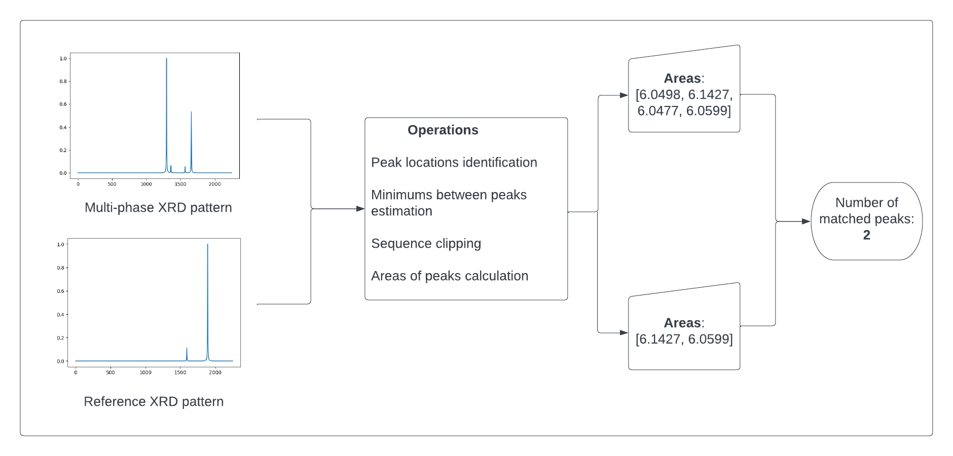
Figure 1: Peak matching algorithm overview.

3.3 Calibration model

Described framework provides efficient and accurate solution to the problem. However, attempts when the algorithm fails to detect material properly because of overlapping or difficult peaks are not addressed. For this reason, we create an additional support model which uses meta-features obtained from peak matching algorithm to predict materials more precisely.

3.3.1 Models

Performance analysis is conducted for particular supervised learning and ensemble models: Logistic Regression, Support Vector Machine (SVM), k-Nearest Neighbours (kNN), Decision Tree (DT), Random Forest (RF). All of the models were implemented in Scikit-Learn (Pedregosa et al., 2011). To evaluate performance precisely, 5-fold stratified cross-validation strategy was used based on equal distribution of samples with positive and negative matches. Features were additionally normalized by removing the mean and scaling to unit variance. Complete list of features used for training is shown below.

• The number of peaks calculated by the matching algorithm.

• The first index on which the condition $s_{i}>0$ is true.

• The last index on which the condition $s_{i}>0$ is true.

• The first index on which the condition $x_{i}>0$ is true.

• The last index on which the condition $x_{i}>0$ is true.

• The sum of areas of peaks for multi-phase material.

• Target value: is $x_{i}$ presented in $s_{i}$ or not.

Model	Precision	Recall	F1 Score
No calibration model	0.975	0.772	0.862
Logistic Regression	0.989	0.763	0.861
Support Vector Machine (SVM)	0.991	0.773	0.869
k-Nearest Neighbours (kNN)	0.920	0.834	0.875
Decision Tree (DT)	0.768	0.870	0.816
Random Forest (RF), basic	0.887	0.820	0.852
Random Forest (RF), tuned	0.977	0.813	0.888

Table 2: Experiments showcase and their corresponding scores.

4 Experiments

Rounding point	F1 Score
5	0.875
4	0.888
3	0.614
2	0.349

Table 3: Comparison of performance with different rounding points.

Selected algorithms were trained on data acquired from peak matching. Standard parameters for each model are selected and compared using defined evaluation metrics. Namely, precision, recall and F1-score are used. $\displaystyle F1=2*\frac{Precision*Recall}{Precision+Recall}$, is essentially the harmonic mean of precision and recall. Since the distribution of classes is highly imbalanced, F1 score addresses this problem as balances between precision and recall. Comparison of mentioned methods can be seen in Table 2. It’s noted that some of the models did not beat the baseline without any additional supervised learning algorithm. Theoretically, this might be due to the fact that peaks positions are hard to learn since they can overlap for different pairs of materials. After careful consideration of hyperparameters, random forest with number of trees - 50, increased the maximum depth of the tree to 14 and log loss as the criterion achieves the highest F1 score among other models. Moreover, we have to consider the importance of the rounding value as matching of areas under peaks have significant dependence on it as shown in Table 3.

5 Future work

Described method has its own limitations. Close-set phase identification is still might not be accurately performing on real-world scenarios, where pattern and crystal structure may vary due to the number of reasons including but not limited to the state of diffractometer, previous conducted experiments and the flow of the current experiment. For instance, noise reduction and baseline correction techniques might have to be incorporated to handle more complex cases.

6 Conclusion

In conclusion, machine learning has shown to be a powerful tool for X-ray diffraction (XRD) phase identification. A variety of machine learning algorithms, such as support vector machines, random forests, and k-nearest neighbors, have been applied to analyze XRD patterns and identify different phases in materials by comparing them to a close-set database of XRD patterns. One of the key features used for this analysis is the peak area calculation, which is used to quantify the intensity of the diffraction peaks. This is an important aspect as it allows for more accurate identification of different phases in the XRD patterns. The close-set database of XRD patterns enables the identification to be performed in a more specific and targeted manner, limiting the possibility of misidentification. Presented methods have been effective in identifying phases in small datasets and a limited number of phases, but there is still a need for more robust and accurate methods for XRD phase identification on large datasets. This research highlights the potential of machine learning in XRD phase identification, especially for close-set setups, and suggests directions for future research in this field.

References

- Akiba et al. (2006) E Akiba, H Hayakawa, and T Kohno. Crystal structures of novel la–mg–ni hydrogen absorbing alloys. Journal of alloys and compounds, 408:280–283, 2006.
- Burke (2012) Kieron Burke. Perspective on density functional theory. The Journal of chemical physics, 136(15):150901, 2012.
- Chibani & Coudert (2020) Siwar Chibani and François-Xavier Coudert. Machine learning approaches for the prediction of materials properties. Apl Materials, 8(8):080701, 2020.
- Datta & Grant (2004) Sharmistha Datta and David JW Grant. Crystal structures of drugs: advances in determination, prediction and engineering. Nature Reviews Drug Discovery, 3(1):42–57, 2004.
- Duax et al. (1972) WL Duax, H Hauptman, CM Weeks, and DA Norton. Valinomycin crystal structure determination by direct methods. Science, 176(4037):911–914, 1972.
- Gražulis et al. (2009) Saulius Gražulis, Daniel Chateigner, Robert T. Downs, A. F. T. Yokochi, Miguel Quirós, Luca Lutterotti, Elena Manakova, Justas Butkus, Peter Moeck, and Armel Le Bail. Crystallography Open Database – an open-access collection of crystal structures. Journal of Applied Crystallography, 42(4):726–729, Aug 2009. doi: 10.1107/S0021889809016690. URL http://dx.doi.org/10.1107/S0021889809016690.
- Greasley & Hosein (2022) Jaimie Greasley and Patrick Hosein. Exploring supervised machine learning for multi-phase identification and quantification from powder x-ray diffraction spectra, 2022. URL https://arxiv.org/abs/2211.08591.
- Kaufmann et al. (2020) Kevin Kaufmann, Daniel Maryanovsky, William M. Mellor, Chaoyi Zhu, Alexander S. Rosengarten, Tyler J. Harrington, Corey Oses, Cormac Toher, Stefano Curtarolo, and Kenneth S. Vecchio. Discovery of high-entropy ceramics via machine learning, May 2020. URL http://dx.doi.org/10.1038/s41524-020-0317-6.
- Macrae et al. (2020) Clare F. Macrae, Ioana Sovago, Simon J. Cottrell, Peter T. A. Galek, Patrick McCabe, Elna Pidcock, Michael Platings, Greg P. Shields, Joanna S. Stevens, Matthew Towler, and Peter A. Wood. Mercury 4.0: from visualization to analysis, design and prediction. Journal of Applied Crystallography, 53(1):226–235, Feb 2020. doi: 10.1107/S1600576719014092. URL https://doi.org/10.1107/S1600576719014092.
- Oviedo et al. (2018) Felipe Oviedo, Zekun Ren, Shijing Sun, Charlie Settens, Zhe Liu, Noor Titan Putri Hartono, Ramasamy Savitha, Brian L. DeCost, Siyu I. P. Tian, Giuseppe Romano, Aaron Gilad Kusne, and Tonio Buonassisi. Fast and interpretable classification of small x-ray diffraction datasets using data augmentation and deep neural networks, 2018. URL https://arxiv.org/abs/1811.08425.
- Park et al. (2022) Sun Young Park, Byeong-Kook Son, Jiyoung Choi, Hongkeun Jin, and Kyungbook Lee. Application of machine learning to quantification of mineral composition on gas hydrate-bearing sediments, ulleung basin, korea. Journal of Petroleum Science and Engineering, 209:109840, 2022. ISSN 0920-4105. doi: https://doi.org/10.1016/j.petrol.2021.109840. URL https://www.sciencedirect.com/science/article/pii/S0920410521014595.
- Pedregosa et al. (2011) F. Pedregosa, G. Varoquaux, A. Gramfort, V. Michel, B. Thirion, O. Grisel, M. Blondel, P. Prettenhofer, R. Weiss, V. Dubourg, J. Vanderplas, A. Passos, D. Cournapeau, M. Brucher, M. Perrot, and E. Duchesnay. Scikit-learn: Machine learning in Python. Journal of Machine Learning Research, 12:2825–2830, 2011.
- Suzuki et al. (2020) Yuta Suzuki, Hideitsu Hino, Takafumi Hawai, Kotaro Saito, Masato Kotsugi, and Kanta Ono. Symmetry prediction and knowledge discovery from x-ray diffraction patterns using an interpretable machine learning approach. Scientific reports, 10(1):1–11, 2020.
- van de Streek & Neumann (2014) Jacco van de Streek and Marcus A Neumann. Validation of molecular crystal structures from powder diffraction data with dispersion-corrected density functional theory (dft-d). Acta Crystallographica Section B: Structural Science, Crystal Engineering and Materials, 70(6):1020–1032, 2014.
- Wei et al. (2019) Jing Wei, Xuan Chu, Xiang-Yu Sun, Kun Xu, Hui-Xiong Deng, Jigen Chen, Zhongming Wei, and Ming Lei. Machine learning in materials science. InfoMat, 1(3):338–358, 2019.